Carbon budget concept and its deviation through the pulse response lens

The carbon budget concept states that the global mean temperature (GMT) increase is roughly linearly dependent on cumulative emissions of CO₂. The proportionality is measured as the transient climate response to cumulative emissions of carbon dioxide (TCRE). In this paper, the deviations of the carbon budget from the strict linear relationship implied by the TCRE are examined through the lens of a temperature response to an emission pulse (i.e., pulse response) and its relationship with a nonlinear TCRE. Hereby, two sources of deviation are distinguished: emission scenario and climate state dependence. The former stems from the scenario choice, i.e., the specific emission pathway for a given level of cumulative emissions and the latter from the change in TCRE with changing climatic conditions. Previous literature argues for scenario independence using a stylized set of emission scenarios, and offers a way to fit a nonlinear carbon budget equation. This paper shows how the pulse response, viewed as a Green's function, gives a unifying perspective on both scenario and state dependence. Moreover, it provides an optimization program that tests the scenario independence under the full range of emission pathways for a given set of constraints. In a setup chosen in this paper, the deviations stemming from emission pathway choices are less than 10 % of the overall temperature increase and gradually diminish. Moreover, using the pulse response as a Green's function, the scenario-dependent effects of a reduced-complexity climate model were replicated to a high degree, confirming that the behavior of scenario-dependent deviations can be explained and predicted by the shape of the pulse response. Additionally, it is shown that the pulse response changes with climatic conditions, through which the carbon budget state dependency is explained. Using a pulse response as an approximation for a state-dependent TCRE, an alternative method to derive a nonlinear carbon budget equation is provided. Finally, it is shown how different calibrations of a model can lead to different degrees of carbon budget nonlinearities. The analysis is done using FaIRv2.0.0, a simple climate emulator model that includes climate feedback modifying the carbon cycle, along with a one-box model used for comparison purposes. The Green's function approach can be used to diagnose both models' carbon budget scenario dependency, paving the way for future investigations and applications with other and more complex models.

1 Introduction

The carbon budget concept, or the carbon budget approach, has gained prominence over the last decade due to its ability to determine allowable carbon dioxide emissions leading to a specific global mean temperature (GMT) increase. In essence, it assumes a direct link between the total cumulative carbon emissions and the temperature increase without needing to know the preceding emission pathway. Following the concurrent initial discoveries in the late 2000s (Allen et al., 2009; Matthews et al., 2009; Meinshausen et al., 2009; Zickfeld et al., 2009), the concept received wider recognition after being included in the IPCC AR5 WG1¹ (Stocker et al., 2013) and after being presented as an explicit policy recommendation tool for limiting future climate change in IPCC AR6 WG1 (Table SPM.2) (Masson-Delmotte et al., 2021), where the “remaining carbon budgets” indicate how much carbon may be emitted while still reaching low-temperature targets, assuming net-zero emissions afterward. By and large, since its emergence, the carbon budget has become “a staple of climate policy discourse”, having paved the way for various discourses, from policy proposals and international climate justice discussions to financial recommendations and even climate activism arguments for the immediate abandonment of fossil fuels, to name a few (Lahn, 2020).

Formally, the carbon budget assumes the GMT increases nearly linearly with cumulative emissions, regardless of the preceding carbon emission scenario. Hence, a linear carbon budget equation can be expressed as

$$\begin{array}{}\text{(1)}& T\left(t\right)=\mathrm{\Lambda }F\left(t\right),\end{array}$$

where $F\left(t\right)={\int }_{\mathrm{0}}^{t}E\left(\mathit{\tau }\right)\mathrm{d}\mathit{\tau }$ stands for cumulative emissions and Λ is the proportionality constant, called the transient climate response to cumulative CO₂ emissions (TCRE). The (nearly) linear relationship emerges due to nonlinearities canceling each other out: a concave temperature dependency on the atmospheric carbon content and a convex atmospheric CO₂ dependency on cumulative emissions (Matthews et al., 2009; Raupach, 2013). The former stems from the radiative efficiency saturation of the atmospheric carbon and the latter from the declining ocean heat uptake and the weakening of natural carbon sinks (MacDougall and Friedlingstein, 2015).

When it comes to explicitly determining the remaining budget to reach a certain temperature target, a segmented framework had been devised by Rogelj et al. (2018). In essence, it determines what quantity of cumulative emissions will lead to a given level of peak warming if historical, non-CO₂, and zero emission commitment (ZEC) warmings are subtracted. ZEC is another metric closely related to TCRE and measures the warming (or cooling) that occurs after emission cessation (Matthews and Weaver, 2010). MacDougall et al. (2020) show that different models perform differently, with an inter-model range of ZEC 50 years following the emission cessation being −0.36 to 0.29 K. If ZEC were 0, then there would be no time delay in temperature response, and emissions would directly map to temperature according to TCRE. In reality, there is always some time lag between the input and the climate system's response (e.g., Ricke and Caldeira, 2014). Regardless of ZEC, the linear segmented framework concept itself has been revisited by Nicholls et al. (2020), who show that its assumption of a linear relationship between peak warming and cumulative emissions leads to lower budgets, although this effect is small in the context of other uncertainties.

Hence, there is evidence that the relationship between the temperature and cumulative emissions (Eq. 1) can be nonlinear, as either of the two (convex or concave) mechanisms mentioned above could hypothetically outweigh the other under higher climatic stress (higher T). Indeed, Gillett et al. (2013) show that the linear relationship overestimates temperature response in most Earth system models (ESMs). Using the FaIR simple climate model (SCM), Leach et al. (2021) quantify the TCRE drop to approximately 10 % per 1000 PgC. Additionally, Leduc et al. (2015) have shown that constant TCRE is a good approximation for temperature response under low-emission scenarios, while it overestimates the model's response to high-intensity scenarios; this reaffirms the need for TCRE to decrease in order for the relationship in Eq. (1) to hold true. In the extant literature, Nicholls et al. (2020) have derived the nonlinear carbon budget equation by positing a logarithmic relationship between cumulative emissions and temperature increase with a multiplying factor that allows the relationship to be both convex and concave. In this paper, the change in TCRE with changing climatic conditions is referred to as (climate) state-dependent carbon budget deviation.

Further on, an alternative source of deviation from the budget approach that stems only from the choice of emission scenario, and not from the initial and final climate conditions of the system, is possible. In this paper, this type of deviation is referred to as an emission-scenario-dependent carbon budget deviation. Previous literature, utilizing high-complexity climate models (ESMs), tends to argue in favor of scenario independence (Gillett et al., 2013). However, the problem with using ESMs to study the emission scenario effects is that these models are very costly from a computational standpoint, which means only a limited set of emission pathways are examined. Using a climate model of intermediate complexity, Herrington and Zickfeld (2014) tested the robustness of the scenario independence with a set of 24 emission scenarios. Millar et al. (2016) addressed this problem by forcing the simplified, globally aggregated climate model under various emission scenarios. However, to the best of the author's knowledge at the time of writing, the entire portfolio of emission scenarios that would yield the extreme cases of maximum possible scenario-dependent carbon budget deviations has yet to be investigated and scrutinized.

There is evidence that state- and scenario-dependent deviations are conditional on the model's complexity (MacDougall, 2017), suggesting that models with low linearity have a higher path dependence and vice versa. In this paper, the two effects are approached as separate entities, as the emission scenario-dependent carbon budget deviation implies the possibility of achieving a different temperature T by following a different emission pathway with the same total cumulative emissions F. On the other hand, it is exactly the change in F (and consequently T) that drives the state dependency of TCRE. As will be shown in this paper, with conclusions restricted to the model inspected, one can have one without the other, with the conditions given explicitly.

At its core, this study is focused on conducting a thorough assessment of deviations within the carbon budget approach, encompassing both scenario- and state-dependent deviations. The study introduces a novel concept termed the “pulse response representation”, referring to the analysis of a temperature response to an emission pulse, under different climatic conditions. This conceptual framework proves to be a convenient and effective tool for explaining the observed deviations.

A reinterpretation of the carbon budget equation is suggested using a pulse response in the context of the Green's function equation. It is shown that the linear carbon budget equation is only a special case of the Green's function equation. More importantly, the paper demonstrates that, by utilizing the pulse response as a Green's function, one can capture scenario-dependent deviation effects. Hence, it is revealed that, merely by assessing the shape of the pulse response, one can directly deduce to what extent the model adheres to carbon budget scenario independence.

The Green's function's validity is assessed through an optimization program functioning as the generator of scenario-dependent deviations. Specifically, the optimization program empowers users to assess the entire portfolio of emission scenarios, generating extreme cases of maximum scenario-dependent deviations within user-defined constraints. As such, the optimization program provides an enhanced approach in contrast to previous literature that tests predefined scenario sets instead.

Moreover, the paper translates the changing pulse response under varying climatic conditions into a state-dependent TCRE. The state-dependent TCRE, once explicitly quantified, is used to develop a nonlinear carbon budget equation. This equation is capable of replicating the temperature dynamics seen in a reduced-complexity climate model, also referred to as a simple climate model (SCM). Therefore, it is shown that one can deduce the model’s degree of carbon budget nonlinearity, only by examining its pulse response. Moreover, it is an alternative way of deriving the nonlinear carbon budget equation to that put forward by Nicholls et al. (2020). The novelty of the method given in this paper is that a user does not assume any functional form but derives the change in TCRE from the change in the pulse response under changing climatic conditions.

Lastly, the paper shows how different parameterizations of the model lead to different behavior of the pulse response. Using the same logic as with inspecting the state-dependent TCRE, it is explained how the pulse response representation reveals whether a specific model's parameterization leads to a concave, convex, or linear carbon budget equation. This comes with a caveat since only a very limited parameter space has been inspected and the equation has been derived for only one parameter set. While the indications are clear, the validation across a larger parameter space is left for future work.

Overall, this paper offers a fresh perspective on how to approach the carbon budget and its deviations through the pulse response lens. It presents the pulse response in the role of a Green's function, providing a unifying view of both the scenario dependence and state dependence of the carbon budget approach.

The paper is arranged as follows. In Sect. 2, the models are introduced and the Green's function framework is connected with the carbon budget equation. In Sect. 3, the pulse response representation in the context of Green's function is inspected and its implications for scenario- and state-dependent deviations are revealed. Additionally, Sect. 3 provides a method to derive a nonlinear carbon budget equation using a changing pulse response as an approximation for state-dependent TCRE. In turn, Sect. 4 introduces the optimization program which generates the upper-boundary scenario-dependent deviations and validates Green's approach; also, the nonlinear budget equation is tested against the corresponding SCM. In Sect. 5, the findings are discussed in a broader context, followed by conclusions provided in Sect. 6.

2 Models

The numerical optimization procedure introduced in Sect. 4. used to validate the Green's approach and generate carbon budget deviations requires a substantial number of model runs, so a computationally efficient model is a necessary choice. Hence, the analysis is restricted to a class of simple climate models, also known as climate emulators or reduced-complexity climate models. I distinguish between and apply two approaches, the SCM approach and its corresponding Green's function approach. While the former is sufficient for numerical assessment of the carbon budget deviations, the latter mathematically formalizes the carbon budget approach and offers a fresh perspective on the deviation through the pulse response representation. All of the runs are executed in the GAMS programming language, and the code for the models is available online (https://doi.org/10.5281/zenodo.8314808, Avakumović, 2023).

2.1 FaIR model

By FaIR, I am referring to the FaIRv2.0.0 model as provided by Leach et al. (2021). Cross-Chapter Box 7.1 in IPCC AR6 WG1 argues in favor of FaIR's value as a climate emulator (Forster et al., 2021). For the purposes of this paper, two features of FaIR are crucial. The first is its ability to correctly capture the temperature response following a single carbon emission pulse, i.e., pulse response (Millar et al., 2017); the second is its ability to incorporate climate feedback on the carbon cycle, with one of the effects being the modification of the changing pulse response with changing climatic conditions.

In essence, the FaIR model is an SCM designed to emulate the gas dynamics of different radiative forcers and their effect on the global mean temperature. Because I am interested only in the deviations from the carbon budget, the non-CO₂ forcers are left out of the analysis, utilizing only the carbon cycle system and its radiative forcing dynamics. The model's description and equations can be found in Leach et al. (2021).

FaIRv2.0.0 consists of four carbon and three temperature components. Each carbon component has an associated decay timescale which dictates the dissipation of the carbon content into the shared permanent pool that represents the natural global carbon sink. Along with the global temperature increase, the sink's increased content creates a feedback mechanism, resulting in increased decay timescales and, therefore, increased atmospheric CO₂ retention time. The atmospheric concentration gives rise to radiative forcing by combining a logarithmic and square root term, which translates into the temperature increase distributed between the components. Unless explicitly stated otherwise, FaIR is implemented with its default parameterization, with the default thermal and carbon cycle feedback parameters provided in Leach et al. (2021) and with the default carbon cycle parameters presented in Millar et al. (2017).

The effect of parameter uncertainty is addressed via a set of six FaIR calibrations. The parameters can be found in Tables 2 and 3 in Leach et al. (2021), representing the thermal and carbon cycle feedback parameters tuned to CMIP6 models. Specifically, the sets used in this paper are tuned to the models MIROC-ES2L (Hajima et al., 2020), BCC-CSM2-MR (Wu et al., 2019), MPI-ESM1-5 (Müller et al., 2018), CNRM-ESM2-1 (Séférian et al., 2019), and ACCESS-ESM1-5 (Ziehn et al., 2020).

2.2 The one-box model

To see how drastically different pulse response affects the deviation, another SCM is introduced into the analysis. Employed as a climate module in climate-economy integrated assessment models like FUND (Anthoff and Tol, 2014), PAGE (Hope, 2006), and MIND (Edenhofer et al., 2005), the one-box model consists of only one carbon and one temperature compartment, and it does not include any climate feedbacks. Since Joos et al. (2013) have shown that three to four timescales attributed to individual compartments are necessary to correctly approximate the redistribution of CO₂ in the atmosphere, the one-box model is not sufficient to imitate ESMs fully. Nevertheless, Khabbazan and Held (2019) have shown that different calibrations can be found with which it can emulate the temperature response of ESMs under RCP scenarios. The model's description and equations can be found in Petschel-Held et al. (1999). In this paper, the thermal parameters were chosen to fit the TCR and ECS values provided by FaIR's default parameterization, with the conversion formulae given in Khabbazan and Held (2019).

Note that FaIR and the one-box model are not on equal footing, as the former is considered a state-of-the-art climate emulator, while the latter does not adhere to the carbon budget approach, as will be shown. Hence, the one-box model’s pulse response should not be considered a correct representation of climate response, but rather a comparison tool. It is introduced in this article precisely because of its inexact pulse response behavior in order to underscore how the pulse response is connected to carbon budget deviations. Also, it allows us to explore the effects of structural model uncertainty.

2.3 The Green's function framework

2.3.1 The Green's function formalism

Green's model is one equation motivated by Green's function formalism. Essentially, a Green's function f_g(t−τ) is a specific function unique to a set of linear differential equations Lx(t)=y(t), where y(t) is the input forcing and x(t) is the state variable that changes according to the forcing and the linear operator L. The advantage of Green's function is that it acts as a “propagator” from the input variable (external forcing) to the output variable (change in state variable), allowing us to replace differential equations with just one equation, which reads as $x\left(t\right)={\int }_{t_{\mathrm{0}}}^{t}y\left(\mathit{\tau }\right)f_{\mathrm{g}}(t-\mathit{\tau })\mathrm{d}\mathit{\tau }$.

Using the same formalism, Green's equation is proposed in the context of global mean temperature dynamics with a climate model in lieu of a set of linear differential equations (see Raupach, 2013). Hence, I propose the following equation, imitating the Green's function formalism:

$$\begin{array}{}\text{(2)}& T\left(t\right)=\underset{t_{\mathrm{0}}}{\overset{t}{\int }}E\left(\mathit{\tau }\right)f_{\mathrm{g}}(t-\mathit{\tau })\mathrm{d}\mathit{\tau }.\end{array}$$

The output variable is the global mean temperature change T(t), and the input (forcing) variable represents the emissions E(t). Green's function f_g(t−τ) modifies the contribution to a current temperature T(t) stemming from the past emissions E(τ). According to Eq. (2), the temperature in time t will depend on each emission contributing at time τ prior to t, with the effect modified by Green's function f_g dependent on how far the emission year τ is from t; hence, f_g(t−τ). Essentially, it is an integration scheme that counts the temporarily modified temperature contributions to each emission pulse, going backwards from moment t, with a resulting temperature being a superposition of modified contributions. Similar approaches can be found in the literature in Shine et al. (2005) and Ricke and Caldeira (2014). The difference is that, in Eq. (2), the temperature is deduced directly from emissions, without the need to quantify the radiative forcing and/or atmospheric CO₂ response.

2.3.2 The pulse response as a Green's function

To make use of Eq. (2), one needs to choose an appropriate shape of Green's function f_g. Following the proposed definition, the chosen function is set to be a temperature evolution response following the 1 PgC emission pulse, or simply the “pulse response”. Therefore, in this paper, the terms “Green's function”, pulse response, and “temperature evolution following the emission pulse” are interchangeable. Pulse response experiments are one of the generic experiments applied when evaluating climate models. As done in previous literature (Joos et al., 2013; Millar et al., 2017), the pulse response is generated by adding a unit emission pulse on prescribed emissions that keep a constant background atmospheric concentration background, as follows.

The model is forced by the idealized RCP6.0 CO₂-only emission scenario provided by the RCMIP protocol (Nicholls et al., 2021), starting from the year 1850. In the year of pulse response generation t_p, the emission pathway necessary to keep the level of atmospheric concentration C_a(t_p) constant is generated. Using the derived emissions, two experiments are run: one with the generated emissions only and one with 1 PgC extra added in t_p. Thus, the pulse response (Green's function) is determined by subtracting the temperature evolution of the two runs.

The pulse response functions generated for different years (and hence different climatic conditions) can be found in Figs. 1a, 1b, and 3 for the FaIR model standard parameterization, one-box model, and different FaIR parameterizations, respectively. In this paper, the set of different pulse responses generated under different climatic conditions is named a pulse response representation. Having a set of pulse responses (a representation) gives us information on both the scenario and state dependency of a particular model, as will be discussed in the next section.

The Green's functions f_g utilized in Green's model (Eq. 2), and used in the optimization programs in Sect. 4, are generated at the year t_p=2020 and depicted in blue in Fig. 1a and b, labeled “pulse2020”.

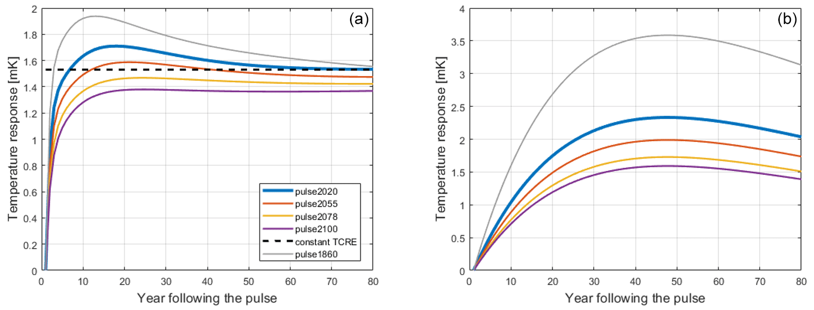
Figure 1 Temperature evolutions in response to 1 PgC emission pulse for different climatic conditions, i.e., pulse responses (colored lines) for FaIR (a) and the one-box model (b), as well as the temperature response implied by Eq. (1) (black dashed line, a). The numbers correspond to the year of an idealized RCP6.0 scenario in which the pulses were generated. The years 2020, 2055, 2078, and 2100 correspond to the FaIR-generated background temperatures of 1, 1.5, 2, and 2.5 K, respectively, and 1860 to preindustrial climatic conditions. Constant TCRE is equal to 1.53 K EgC⁻¹ and corresponds to the central TCRE estimates in Leach et al. (2021) and AR6.

3 Pulse response as a carbon budget deviation indicator

In this section, the theory behind the pulse representation in the form of Green's function and its ability to explicate carbon budget deviations are explored. The scenario dependency is connected to the shape of the pulse response, whilst the state dependency is connected to changing of the pulse response under changing climatic conditions. The conclusions are validated numerically in Sect. 4. Firstly, the connection between the Green's function (Eq. 2) and carbon budget equation as suggested by Eq. (1) is examined, showing that the latter is merely a special case of the former.

3.1 The carbon budget equation in the context of Green's formalism

Essentially, the linear carbon equation (Eq. 1) suggests an immediate temperature response to (cumulative) emissions, with the response that does not change in time or with climatic conditions. This implies that the pulse response introduced in the previous subsection should also be a constant function. In Fig. 1a, it is plotted as a dashed black line. Formally, a linear budget pulse response can be interpreted as a Heaviside function Θ(t) multiplied by a constant equal to Λ representing TCRE:

$$\begin{array}{}\text{(3)}& f_{\mathrm{g}}^{\mathrm{0}}(t-\mathit{\tau })=\mathrm{\Lambda }\mathrm{\Theta }(t-\mathit{\tau })=\left\{\begin{array}{ll}\mathrm{0}& t<\mathit{\tau }\\ \mathrm{\Lambda }& t\ge \mathit{\tau }\end{array}\right.,\end{array}$$

where τ is the timing of the emission pulse and is equal to the 0th year in Fig. 1.

Proving that the Green's formalism can be considered an analog to the carbon budget approach is simple. Inserting the idealized budget Green's function into Eq. (2), one arrives precisely at the linear budget equation (Eq. 1):

$$\begin{array}{rl}T\left(t\right)& =\underset{t_{\mathrm{0}}}{\overset{t}{\int }}E\left(\mathit{\tau }\right)f_g^{\mathrm{0}}(t-\mathit{\tau })\mathrm{d}\mathit{\tau }=\underset{t_{\mathrm{0}}}{\overset{t}{\int }}E\left(\mathit{\tau }\right)\mathrm{\Lambda }\mathrm{\Theta }(t-\mathit{\tau })\mathrm{d}\mathit{\tau }\\ & =\mathrm{\Lambda }\underset{t_{\mathrm{0}}}{\overset{t}{\int }}E\left(t^{\prime }\right)\mathrm{d}{t}^{\prime }=\mathrm{\Lambda }F\left(t\right).\end{array}$$

Therefore, if the temperature response always had the same (constant) shape as the dashed line in Fig. 1, regardless of the underlying climatic conditions, the carbon budget would not show deviations – each unit of carbon emission would immediately add to the warming equally and regardless of when it was emitted. However, as shown in Fig. 1, the FaIR-generated pulse responses are not a constant function, a fact that has implications for the carbon budget deviations.

3.2 Pulse response shape as a scenario dependency indicator

For now, the focus is on the pulse response functions used in Green's model (pulse 2020, Fig. 1a). In contrast to a constant step function, the initial response at the year of the emission pulse is zero. Then it steeply increases until reaching a maximum value of approximately 1.7 K, roughly 17 years following the pulse. Furthermore, following the peak, there is a slow relaxation of the response, which slowly reaches a constant response later in time.

To get a better feel for the deviations and how they are connected to the pulse, one can consider an extreme example. Say that all of the emissions are injected in one year. Total cumulative emissions will then amount to the value of the emissions injection only. Due to the pulse response, the temperature response will depend on what point in time the observer is at. Tracing the pulse response evolution, we can see a minimum magnitude of temperature in the first year of the pulse and the maximum temperature at the peak of the response, ∼17 years after the pulse. Effectively, these are two very different temperatures for the same cumulative emissions. The difference between the two temperatures is the maximum possible scenario-dependent carbon budget deviation. If the cumulative emissions then amount to 100 PgC, the pulse response scales accordingly, and the theoretical deviation between the minimum and maximum response is ∼ 0.17 K.

Finally, because of the gradual relaxation of the response, if the year in question is far enough from when I maximized the deviation, the deviation itself diminishes. In the extreme case presented in the previous paragraph, this can be intuitively seen as follows. Although there could have been a considerable difference in temperature stemming from the same cumulative emissions between the 0th (the injection year) and 17th year (the peak year) following the pulse, going forward in time, the temperature response difference between the 80th and 63rd year following the pulse (again, a 17-year difference) is virtually nonexistent. Hence, the carbon budget deviation “fixes” itself as the system enters dynamic relaxation, i.e., the pulse response reaches a nearly constant value. Once it reaches the relaxation phase, the pulse response becomes very similar to the step-function response of the linear budget.

The Green's function derived from the one-box model is shown in Fig. 1b (blue). Unlike its FaIR counterpart, the one-box model's pulse response peaks much later (roughly 45 years after the pulse). Additionally, and more importantly, it never reaches the relaxation phase in the form of a constant response in later years; it starts permanently decreasing after the peak instead. In the context of the discussion above, this means that, aside from its magnitude, even the sign of the one-box model's scenario-dependent deviations can change depending on the relative time we observe it. Repeating the thought experiment above, where I emit everything in one year, the observer will see a positive deviation when comparing the initial (injection) year and the peak year (∼ 45-year difference). If we go forward in time, specifically 45 years further, the observer who was in the initial year now sees their temperature response at the peak, while the observer who was in the peak temperature year now sees a much lower temperature. Subtracting the two now yields a negative value, even though the deviation was previously positive.

In summary, the pulse response shape dictates both the deviation and its evolution, making it critical for the climate model's adherence to the carbon budget approach and its emission scenario independence. The FaIR model shows small, scenario-dependent deviations precisely because its pulse reaches an almost constant regime relatively quickly following a peak. Moreover, if a model cannot emulate reaching the temperature relaxation, it will also show much higher and, more importantly, time-dependent and emission-scenario-dependent deviations.

3.3 Pulse response alteration as a state dependency indicator

Until now, only a single pulse response (pulse2020) has been employed as Green's function and examined. However, the experiment shows that this pulse response changes with changing climatic conditions: following the same procedure described in Sect. 2.3.2, pulse responses are generated later in the RCP emission run for different t_p values accordingly. The generated pulses are depicted in different colors in Fig. 1 for both the FaIR and one-box models. The further analysis considers only the FaIR results, as the one-box model fails at criteria of pulse response relaxation, as explored in the previous subsection.

When comparing the pulses (Fig. 1a), a general trend can be recognized. As the system is subjected to higher climatic stress in the form of higher cumulative emissions and higher temperatures, both the shape and the magnitude of the pulse response change. While all the pulse response variations show the aforementioned steep increase in the first few years following the pulse, the magnitude of the peak and the corresponding relaxation temperature level decrease with changing climatic conditions, with a visible “flattening” of the curve.

3.3.1 State-dependent pulse response as a variable TCRE

As discussed in the Introduction, previous literature suggests that TCRE is not a constant value but slowly decreases with cumulative emissions. This can be interpreted as the carbon budget's state dependency, which manifests in the nonlinear carbon budget equation (Nicholls et al., 2020). This nonlinearity can be identified by examining the change in pulse response shape with changing background climate conditions.

At the beginning of Sect. 3, it was shown how the step-function pulse response in Green's model translates into TCRE included in Eq. (1). If the TCRE changes with background conditions, the carbon budget step-function pulse (black dashed line, Fig. 1) should also change in magnitude following the climatic stress. Indeed, Fig. 1 shows that the FaIR-generated pulse response decreases in magnitude with background conditions. If the changing pulse is then approximated with a changing step function, the decrease in the pulse response can be directly linked to the decrease in TCRE. A method for using a pulse response representation to explicitly quantify TCRE dependency on climatic conditions is developed, as follows.

To generalize the analysis, the additional pulses are generated under RCP4.5 and RCP8.5 emission scenarios, along with the already generated pulse responses under different climatic conditions under RCP6 (Fig. 1). The first pulse of each run is generated at the benchmark year 2020 and the rest at the same temperature levels (1.5, 2, 2.5 K), where possible.

Next, recalling the linear budget discussion, the generated pulses are to be approximated with the step function. Ignoring the temperature evolution dynamics in the early years of the pulse response, the pulse is transformed into a constant Λ_v by averaging it between years 70 and 80². As shown in Fig. 1, the pulse dynamics relax by that time, reaching relative constancy. With that approximation, however, the ability to express the time delay and scenario dependency is lost, as the shape of the pulse response function dictates the scenario dependency (Sect. 3.2). As they will be shown to be small, this aspect can be safely ignored.

After approximating the pulses, the corresponding cumulative emissions and temperature values (i.e., the background climatic conditions under which the original pulse was generated) are assigned to each value of generated Λ_v. By doing so, the Λ_v(T,F) dependency is mapped, which, when reasoned in line with Eq. (1)³, can be considered a TCRE dependent on cumulative emissions and temperature increase, or simply state-dependent TCRE.

In this way, the carbon budget's state dependency is made explicit: examining each RCP case separately shows that Λ_v decreases linearly in T under the standard FaIR parameterization (Fig. 2b). Moreover, looking at the right figure, one can see that by adding 1 EgC into the system, Λ_v(F) drops by roughly 10 %, which is in keeping with the findings of Leach et al. (2021).

Figure 2 (b) TCRE approximations Λ_v(T) generated from pulse response functions under different climatic conditions and emission scenarios. Scatter plots are actual values of Λ, while the line is the result of linear regression. The different colors represent the Λ_v generated from different RCPs, which are plotted in (a).

3.3.2 From pulse response to carbon budget equation

The RCP6-generated Λ_v (Fig. 2b, yellow dots) is chosen to derive the carbon budget's state dependency from the pulse response representation. The choice of RCP scenario does not constrain the conclusions of this exercise. Figure 2b suggests a linear relationship ${\mathrm{\Lambda }}_v\left(T\right)=-a\cdot T+b$, with a=0.1083 EgC⁻¹ and b=1.646 K EgC⁻¹ derived via linear regression. Therefore, TCRE (here Λ_v) is reinterpreted through the lens of T dependency, as temperature is the main thermodynamic variable driving the climate system change. This way, assuming any functional form for the state dependency is avoided; rather, it is deducted from mapping Λ_v(T) (Fig. 2b). The assumed linear relationship between TCRE and T suggests that TCRE can go to very low and even have negative values due to the negative linear coefficient. However, the linear form is derived and holds true for the values below 2400 PgC (approximately the cumulative emissions in the RCP8.5 scenario at the year 2100). Hence, its domain of applicability is constrained within the theoretical TCRE bounds of 2000 PgC. Additionally, one can see that the assumed linear relationship suggests TCRE would reach zero at roughly T=15 K, well above any projected future temperature increase.

Since Λ_v is, by definition, a temperature response to an emission pulse, the temperature change following the approximated pulse is interpreted as $\mathrm{\Delta }T=\mathrm{\Lambda }\left(T\right)\cdot E_{\mathrm{pulse}}$. In words, the temperature change is equal to one unit of pulse emission scaled by temperature response to a pulse Λ_v. Given the fact that the emission pulse brings about a change in cumulative emissions, the aforementioned relation is rewritten in differential form as

$$\begin{array}{}\text{(4)}& \mathrm{d}T=(-a\cdot T+b)\mathrm{d}F.\end{array}$$

By integrating Eq. (4), one arrives at

$$\begin{array}{}\text{(5)}& T\left(F\right)={\displaystyle \frac{b}{a}}+\left(T_{\mathrm{0}}-{\displaystyle \frac{b}{a}}\right)e^{-a(F-F_{\mathrm{0}})},\end{array}$$

with T₀ and F₀ being the initial values at the time of the first pulse (pulse2020). Essentially, Eq. (5) represents a nonlinear carbon budget equation under a default FaIR parameterization. The validity of the equation is tested in Sect. 4.

When plotted, one can see that T(F) is a closely linear, slightly concave function within the F domain of interest⁴. Concavity comes from the (linearly) decreasing Λ_v(T) (Fig. 2b). If, conversely, Λ_v(T) increases with increasing T, the same derivation method as presented above would lead to a convex carbon budget equation. As will be shown in the next subsection, this is possible, as the pulse response, and subsequently Λ_v(T), evolves differently under different FaIR parameterizations.

3.4 Uncertainty in pulse response

By considering the pulse response representation and its implications for the carbon budget framework under one FaIR parameterization, the effects of different model calibrations on pulse response and, thereby, the carbon budget are evaluated in the final part of this section.

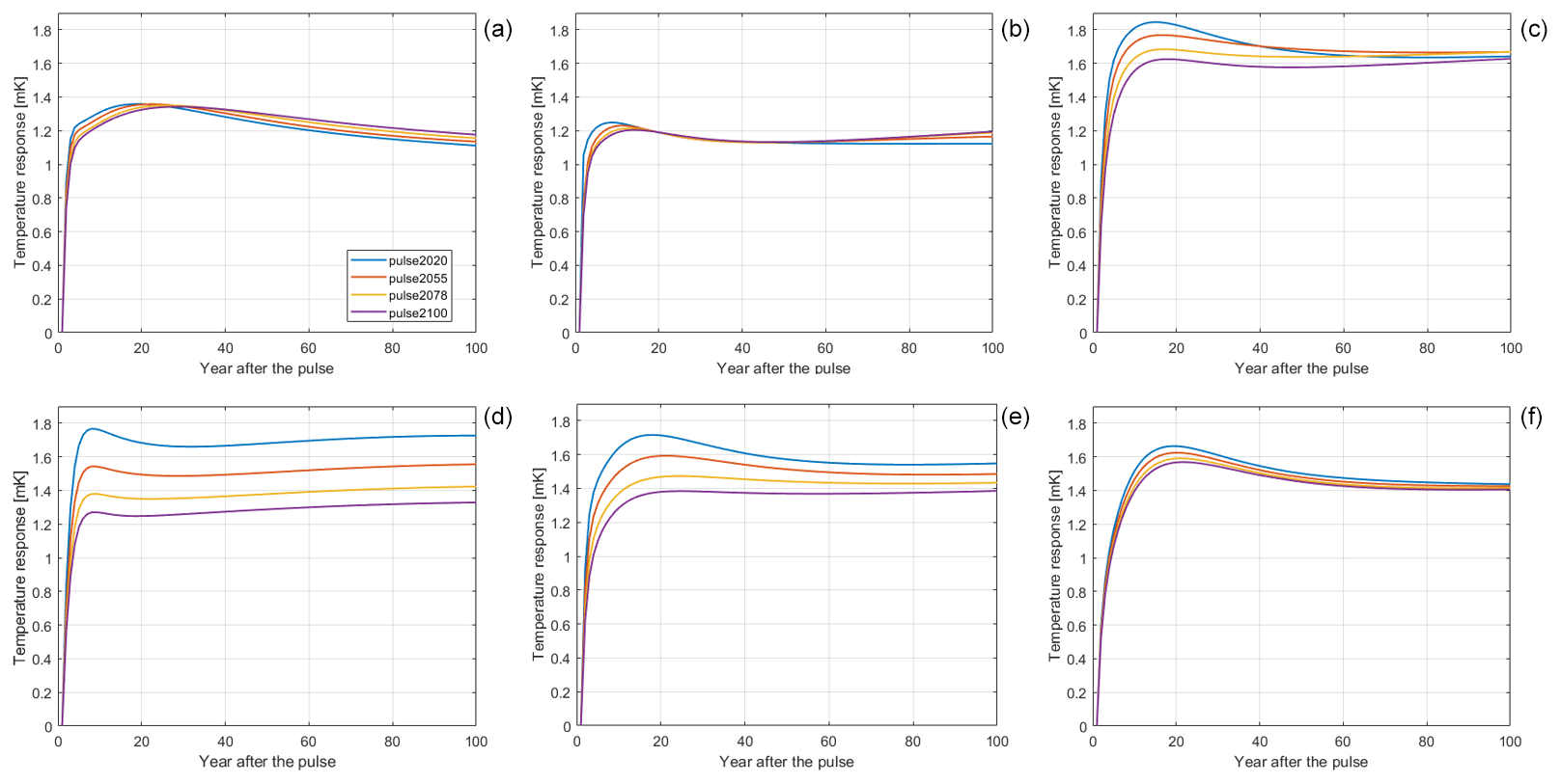
Figure 3 Pulse responses under different FaIR calibrations: MIROC-ES2L, BCC-CSM2-MR, MPI-ESM1-2-LR, ACCESS-ESM1-5, default parameterization, and CNRM-ESM2-1, respectively. Different parameter sets are each tuned to a specific ESM, with parameter values given in Tables 2 and 3 in Leach et al. (2021). Note that (e) matches Fig. 1a, included here for comparison.

Figure 3 shows pulse responses generated as described in Sect. 2.3.2 under six different sets of FaIR parameters, each tuned to a different CMIP6 model, with Fig. 3e being the default parameterization used in the rest of the analyses. We can see that every calibration yields a distinct pattern of behavior. Using the framework introduced in the previous parts of this section, one can deduct how each calibration affects FaIR's adherence to the carbon budget approach.

To examine scenario dependency, one must examine pulse response shape (Sect. 3.2). Looking at Fig. 3, we can see that all of the parameterizations show a relatively small scenario dependency, as all of them show pulse responses that peak in 10–20 years, followed by some degree of relaxation in the time domain of interest. In other words, one can imagine approximating them with a step function. Two parameterizations that stand out are MIROC-ES2L and ACCESS-ESM1-5. The former reaches a peak and then continually decreases just like the one-box model, although at a much slower rate (Fig. 1b). Hence, the scenario-dependent deviations will not fully diminish and are likely to change sign. In the case of the latter, the pulse response never reaches a relaxation state as the temperature continues increasing later in time.

In the context of state-dependent deviations, Fig. 3 reveals an interesting effect of different FaIR parameterizations on the nonlinearity type of carbon budget equation. In Sect. 3.4, it was shown that the changing TCRE under different climatic conditions can be reinterpreted as the changing pulse response through Λ_v(T). Additionally, it was shown that a decreasing Λ_v(T) (Fig. 2b) leads to a concave nonlinear carbon budget equation (Eqs. 5 and 6). The opposite also holds true: if Λ_v(T), and hence the pulse response, increases in magnitude with higher temperatures, it results in a convex nonlinear carbon budget equation. Ultimately, if the pulse response magnitude does not change with changing background conditions, the carbon budget equation is indeed linear⁵. With that in mind, one can easily deduce that not all the combinations of FaIR parameters lead to the concave carbon budget equation, as derived in Eq. (6). For example, MIROC-ES2L tuned to FaIR indicates a slightly convex budget equation, while BCC-CSM2-MR and CNRM-ESM2-1 are closest to the linear carbon budget, and ACCESS-ESM1-5 shows larger concavity than the default FaIR setup inspected in the previous subsection.

Due to the constrained set of fully accessible parameter sets given in Leach et al. (2021), only six calibrations are presented here. A larger set would provide some insights into which parameters in FaIR drive which types of behavior. Additionally, it would be interesting to see to what extent FaIR tuned to a CMIP6 model reproduces the pulse response representation behavior of its corresponding ESM under the same setup. To do so, one needs to run the pulse response experiments (Fig. 3) with ESMs. If it were found to do so, one could potentially extend the pulse response framework with FaIR tuned to ESMs to analyze carbon budget deviations as produced by the corresponding ESM.

4 Numerical evaluation

In the previous section a theoretical background for inspecting carbon budget deviation through the lens of pulse response was established. The shape of the pulse response function is assumed to give information about the model's scenario-dependent deviations, and the method for deriving the nonlinear carbon budget equation from the changing pulse response with changing climatic conditions is provided. In the first brief part of this section, the state-dependent (nonlinear) carbon budget equation is tested against its linear counterpart and FaIR. For the rest of this section the results of using an optimization scheme are presented. Using the optimization scheme in this context has a twofold role. Firstly, the pulse response's ability to capture scenario-dependent effects in the role of a Green's function is confirmed with comparison to the corresponding SCM, validating the hypotheses given in the previous section. Secondly, the optimization scheme tests the full portfolio of possible emissions, providing the highest possible scenario-dependent deviation under given constraints.

The Appendix introduces a modification to the Green's function approach that is necessary to compare diagnosed temperatures in the upper panels of Fig. 5 (but not scenario-dependent deviations, lower panels) between Green's approach and the FaIR model. The modification is a temperature leftover from emissions prior to an optimization year and is, in fact, ZEC (Appendix A).

4.1 State-dependent carbon budget equation

To check if Eq. (5) yields correct temperature dynamics, it is tested against the FaIR model under the aforementioned RCP scenarios. The resulting temperature pathways are plotted in the top row of Fig. 4 (red) alongside the FaIR output (blue) and the linear carbon budget Eq. (1) with two values of constant TCRE (yellow), while the bottom row shows the corresponding relative deviations from the FaIR-generated temperature pathway. The two TCRE values are TCRE${}_{v\mathrm{1}}=\mathrm{1.6}\times {\mathrm{10}}^{-\mathrm{6}}$ K PgC⁻¹ and TCRE${}_{v\mathrm{1}}=\mathrm{1.53}\times {\mathrm{10}}^{-\mathrm{6}}$ K PgC⁻¹.

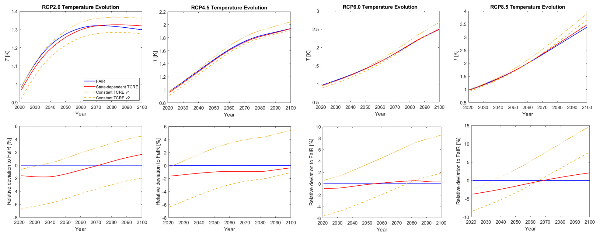
Figure 4 Top row: temperature evolution under three RCP emission scenarios, calculated by the FaIR model (blue), the derived nonlinear carbon budget equation (Eq. 6) (red), and the linear carbon budget equation (Eq. 1 with two different TCRE values) (yellow). Bottom row: corresponding relative deviations of temperatures from FaIR-generated temperature, in percentages.

Choosing a larger constant TCRE (v1) results in a more accurate temperature diagnosis in the first half of the century under lower cumulative emissions, with deviations increasing in step with rising emissions. The opposite is true for a smaller TCRE. In this sense, Eq. (1) with a constant TCRE is a linearized version of FaIR in a similar way as the Green's function model but without the ability to generate scenario-dependent effects. Additionally, we can see that the state-dependent deviations are not transient like their scenario-dependent counterparts, but ever-increasing with the changing cumulative emissions. The highest detected absolute deviation is around ∼0.5 K for the end-of-the-century temperatures in the RCP8.5 run, which amounts to ∼15 % relative deviation from the FaIR-generated temperature.

Unlike constant TCRE, Eq. (5) replicates the FaIR-generated temperatures in the RCP2.6, RCP4.5, and RCP6 runs relatively well, with the relative deviation from FaIR being less than ∼2 % throughout the century. The largest absolute drift from the FaIR-generated temperature is around 0.1 K at the end of the century under the RCP8.5 scenario. However, this degree of drift is less than 3 % in relative terms. Since RCP8.5 is arguably somewhere in the upper bound for possible emission pathways (and RCP2.6 arguably a very optimistic lower bound scenario), one can conclude that Eq. (5) is a good emulator of FaIR under the single default parameterization. The incorporation of different climate parameters in Eq. (5) lies beyond the scope of this paper.

4.2 Scenario-dependent deviations

4.2.1 Optimization scheme

To test upper-bound scenario-dependent carbon budget deviations, the optimization program is formulated as follows:

$$\begin{array}{}\text{(6)}& \begin{array}{rl}& \underset{\mathit{\left\{}E\right(t\left)\mathit{\right\}}}{\left(\mathrm{Max},\mathrm{Min}\right)}\left[T\right(t^{*}\left)\right]\mathrm{s}.\mathrm{t}.\underset{t_{\mathrm{0}}}{\overset{t^{*}}{\int }}E\left(t\right)\mathrm{d}t=F_{\mathrm{tot}},\\ & \left|{\displaystyle \frac{\mathrm{d}E\left(t\right)}{\mathrm{d}t}}\right|\le k,E\left(t\right)\ge \mathrm{0},E\left(t_{\mathrm{0}}\right)=E_{\mathrm{0}}.\end{array}\end{array}$$

The program maximizes (or minimizes) the temperature variable in a given optimization year t^*. The minimum T_min(t^*) and maximum T_max(t^*) temperatures generated provide the upper and lower bounds for possible temperatures under given constraints. The maximum possible scenario-dependent carbon budget deviation T_d is then calculated by subtracting the two boundary temperatures, $T_{\mathrm{d}}\left(t^{*}\right)=T_{\text{max}}\left(t^{*}\right)-T_{\text{min}}\left(t^{*}\right)$.

In the optimization program (Eq. 6), the emission pathway assumes the role of the free control variable, except in the fixed initial condition E(t₀)=E₀. Hence, the novelty of testing scenario independence with the optimization program is that the emission pathway is generated, instead of being assumed as an input by the user. This way, the analysis does not rely on a limited number of emission scenarios but systematically runs through the whole portfolio of possible scenarios under given constraints. Three boundary conditions are implemented, whose values are subjectively chosen by the author so that they provide a set of possible (not necessarily plausible) emission pathways. Restriction on total cumulative emissions F_tot ensures the same quantity of cumulative emissions at the end of the each run so that deviations stem only from scenario choice. The slope restriction k provides a bound on allowed emission change per year. The choice of boundary conditions and run configuration is further described in the Supplement (Sect. S1).

Additionally, two different cases of scenario-dependent deviations are diagnosed and described in the Supplement. The “net-zero” case assumes that the emissions reach zero and that there are no emissions following the optimization year, while the “transient budget” case allows emissions to evolve freely afterwards and allows emissions to take any value in the optimization year.

4.2.2 Transient budget deviation

In Fig. 5, the results of the optimizer in $t^{*}=\mathrm{2090}$ for four different F_tot choices in a transient budget setup are presented, explicitly showing the generated T_max(t^*) and T_min(t^*) dependent on k in the top row and their corresponding T_d(t^*) values in the bottom row. Note that F_tot is counted from the year t₀=2020 and not from preindustrial times like the variable F. For example, F_tot of 416 PgC, in addition to the pre-2020 emitted CO₂, amounts to 1000 PgC, which approximately corresponds to the carbon budget allowed for adhering to a 2 K increase with 67 % probability, as suggested by the IPCC (Masson-Delmotte et al., 2021, Table SPM.2)⁶.

Figure 5 Top row: T_max (red) and T_min (blue) generated by the optimization program for the transient budget case, dependent on k, set up for different total cumulative emissions levels F_tot and $t^{*}=\mathrm{2090}$, with F_tot counted from the initial optimization year t₀=2020. The graphs are ordered by the magnitude of the associated F_tot. The y-axis domains all share the same relative interval of 0.3 K but different absolute values. Lower panels: corresponding scenario-dependent deviations T_d plotted against the respective k values. In all graphs, the solid lines represent the FaIR output; the dashed lines represent Green's output.

Comparing the dashed and solid lines reveals that Green's approach using the pulse response as a Green's function diagnoses both T_max and T_min⁷, as well as scenario-dependent deviations, exhibiting deviations of the same order of magnitude as FaIR, with the Green's function approach being especially close to FaIR for lower cumulative emissions.

When comparing the effect of increasing cumulative emissions in Fig. 5, some notable effects can be identified.

First, T_d(k) increases with higher cumulative emissions, in combination with the increase due to increasing allowed emission slope k. A comparison of the top to bottom graphs shows that the deviation increases by roughly 60 %, in connection with the F_tot increase from 416 to 1000 PgC. In the most extreme case with associated F_tot=1000 PgC, a deviation of ∼0.15 K, roughly 6.3 % of overall temperature increase, is produced.

Next, as seen in the top row, the gap between T_max and T_min generated by FaIR and its Green's counterpart steadily increases with higher cumulative emissions F_tot⁸.

Furthermore, as shown in the bottom row, the difference in T_d(k) between the two models also increases with higher F_tot, albeit to a lesser extent. This effect can be attributed to the widening gap between the maximum and minimum temperature of the FaIR approach, which increases its T_d(k) to a larger extent than Green's model (due to the constancy of Green's function). Both effects can be understood through the change in pulse response with changing climatic conditions. Namely, Green's approach uses one single pulse response as a Green's function throughout the run, although the pulse response changes under changing climatic conditions, i.e., higher cumulative emissions. The change in magnitude of the pulse response affects the drift between the T_max and T_min generated by FaIR Green's model, while the flattening of the response peak causes the drift between the diagnosed deviations T_d.

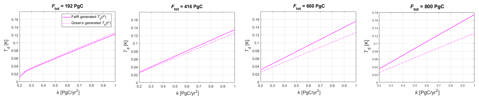
Figure 6 Scenario-dependent deviations, dependent on k, generated by the optimization program for the transient budget case with the allowed negative emissions, dependent on k, set up for different total cumulative emissions levels F_tot and $t^{*}=\mathrm{2090}$, with F_tot counted from the initial optimization year t₀=2020.

4.2.3 Effect of negative emissions

The effect of allowing negative emissions on the transient budget's scenario-dependent deviation is shown in Fig. 6. The figure shows four different combinations of total allowed cumulative emissions F_tot, this time including a choice of F_tot=196 PgC, which, when added to the cumulative pre-optimization emissions, reflects the carbon budget allowed for adhering to 1.5 K with 67 % probability, as suggested by the IPCC (Masson-Delmotte et al., 2021, Table SPM.2). Including negative emissions increases the generated T_d by roughly 0.04 K compared to the zero negative emissions scenario in the highest k case for all F_tot combinations.

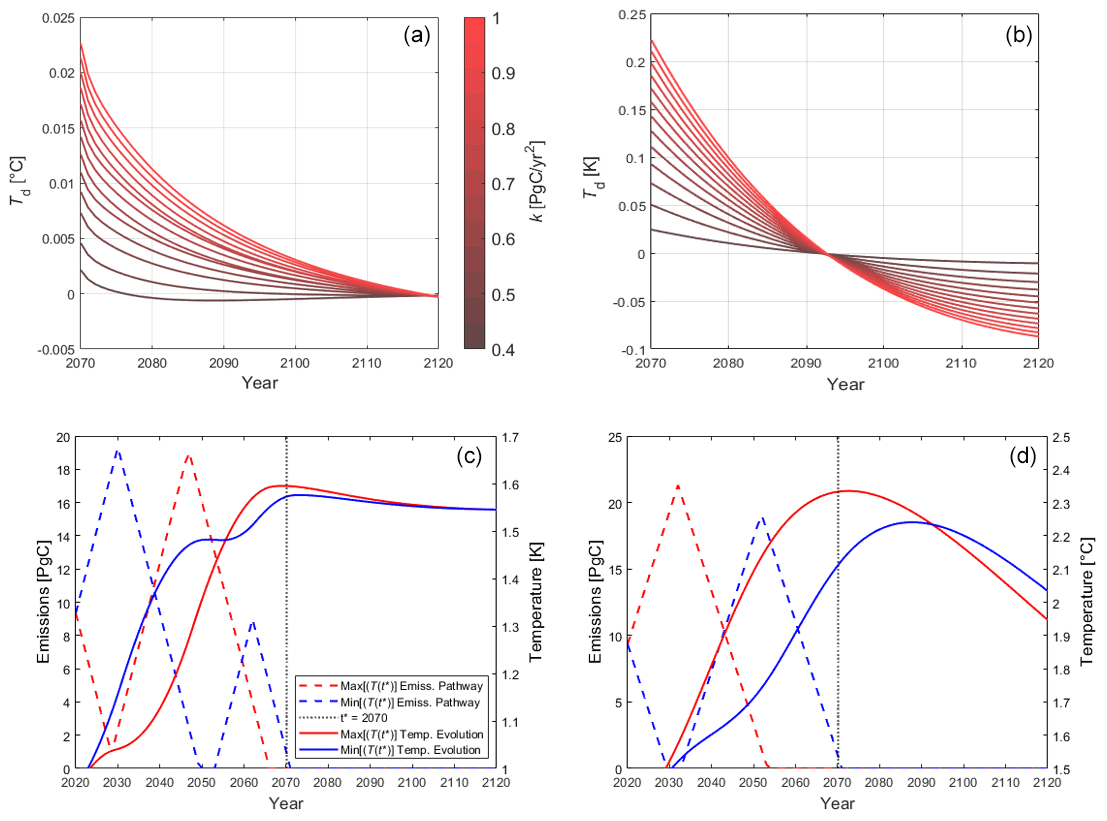
Figure 7 Panels (a) and (b) show the temporal evolution of the net zero-case T_d(k) following the optimization year $t^{*}=\mathrm{2070}$, generated by FaIR and the one-box model, respectively. The colors represent deviations corresponding to the different k allowed, with the darkest red being the lowest allowed (0.4 PgC yr⁻²) and the brightest red being the highest (1 PgC yr⁻²). The generated emission pathways and absolute temperature evolutions corresponding to the optimization runs (both min. and max.) under the same setup for one value, k=1 PgC yr⁻², are shown in (c) and (d), generated by FaIR and the one-box model, respectively.

4.2.4 Scenario-dependent deviation time evolution

Because the optimization program, when set up as a net-zero case, does not allow for emissions following the optimization year, it makes it possible to inspect the time evolution of the generated scenario-dependent deviation T_d(t^*), as there are no further emissions to further modify the temperature.

Figure 7a and b show net-zero generated T_d(t^*) with an additional temporal dimension instead of only k dependence in one year (Fig. 5 lower panels and Fig. 6). In this case, the optimization year is chosen to be $t^{*}=\mathrm{2070}$. The different shades of red depict the k range and their respective scenario-dependent deviations. The chosen F_tot for the run shown in Fig. 7 is 416 GtC.

The net-zero budget case shows a significantly smaller initial T_d(k) than its transient budget counterpart. The difference is due to lower minimum generated temperatures in the transient budget case as a result of a non-constrained E(t^*) and hence allowing emissions to “stack up” at the optimization year, while they are required to reach zero in the net-zero counterpart. The pulse response discussion (Sect. 3) shows that if one wants to maximize the temperature response in a given year, they should stack the emissions ∼17 years before that year; conversely, to minimize the temperature response, they should stack the emissions as close as possible (within given constraints).

Further inspecting Fig. 7a one can notice that, in FaIR, already small scenario-dependent deviations ultimately disappear if no additional carbon dioxide is added to the system; hence, the maximum deviations generated by the optimization program are only temporary. In contrast to FaIR, the one-box model's deviations (Fig. 7b) do not “die out” over time but decrease only to change sign, as predicted in Sect. 3.2.

The deviations' evolutions for k=1 can be backtracked by examining the max. (red) and min. (blue) generated temperature evolutions shown in Fig. 7c and d, as the subtraction of the two yields the T_d(k). The FaIR-generated min. and max. temperature pathways are separated at t^* but eventually coincide, translating to a diminishing carbon budget deviation. Even though two temperatures are generated, they eventually reach the same level, just as the pulse relaxation discussed in the previous section suggests they should. Additionally, their cumulative emissions are equal, meaning that their pulse response is the same, so they reach the same level of constancy following the peak temperature response. The opposite is true for the one-box model counterpart. Because the one-box model's pulse response never reaches relaxation phase, i.e., keeps on decreasing following the peak, it makes a difference when it is emitted.

5 Discussion

To reiterate, this study focuses on evaluating deviations within the carbon budget approach, encompassing both its scenario- and state-dependent aspects. A novel method of analyzing these deviations is proposed in the form of a pulse response representation that explicates and distinguishes both forms of deviations by inspecting the evolution of temperature response to an emission pulse under different climatic conditions. The validity of examining the deviations through the lens of the pulse response has been tested by reinterpreting the pulse response as a Green's function of a set of differential equations that constitute a climate model (Raupach, 2013). Consequently, the introduced optimization program serves a dual role. It supplements the concurrent carbon budget literature by testing a full portfolio of possible, but not necessarily plausible, scenarios for scenario-dependent deviations under given constraints. Additionally, it confirms the ability of Green's function to capture scenario-dependent effects.

The analysis utilizes FaIR, the one-box model, and the associated Green's function models. The nonlinearities appear in FaIR in both the carbon cycle feedback and the temperature response saturation. As pointed out in the Introduction, the interplay between the changing carbon cycle and temperature response produces the near-linearity of the carbon budget equation, with the former being convex and the latter a concave driver of the budget equation.

The second model used in the analysis is the one-box model, introduced as an example of a model with a dramatically different pulse response than FaIR, which facilitates comparison in the context of the pulse response behavior effect on the carbon budget approach deviations. In contrast to FaIR, the one-box model does not include climate feedbacks on the carbon cycle, so nonlinearities arise only through the saturation in temperature response, which means that nonlinearities are solely concave.

Moreover, the inclusion (or lack) of climate feedbacks has an effect on how the pulse response changes with changing climatic conditions. In the one-box model, the carbon cycle response stays the same regardless of background conditions, so the pulse response is modified only by logarithmic temperature response saturation. This manifests in the pulse changing magnitude but not shape. Conversely, including climate feedbacks changes the shape of the response function and modifies its magnitude. For a more detailed discussion on how the climate feedback changes the carbon cycle in FaIR in the context of decreased atmospheric CO₂ decay, see Millar et al. (2017). The effect of convex and concave drivers in the context of pulse response representation and the nonlinearities of the carbon budget equation (Eq. 1) has been examined in Sect. 3.4.

To test whether pulse response behavior offers a trustworthy framework for explaining carbon budget deviations, it is employed as a Green's function in Eq. (2). However, by proposing Eq. (2) and using a FaIR-generated (or one-box-generated) Green's function, I assume that the climate model is a set of linear differential equations. Hence, although Green's model has been proven to capture scenario-dependent effects, the effects of climate change on the carbon budget approach cannot be explicitly captured with Eq. (2). This effect is visible when comparing the FaIR and Green's model optimization runs, as the two sets of generated temperatures have an ever-increasing gap with higher cumulative emissions (Fig. 5, top row). One could modify Eq. (2) so as to include a changing pulse response instead of a fixed f_g, but this remains theoretical; the implementation is unclear.

Regardless of Green's model's inability to correctly forecast (or hindcast, for the same reasons) temperature evolution, Sect. 4 shows that it is indeed capable of mimicking the scenario-dependent deviations of both FaIR and the one-box model. Even though there is an ever-increasing gap between temperatures generated by the SCM and Green's model, the scenario-dependent deviations are well represented by Green's function even for higher F_tot. Hence, one concludes that state and scenario dependencies can arise independently.

The distinction is crucial because nonlinearities in the carbon budget and scenario-dependent deviations are distinct concepts, yet both contribute to carbon budget deviations individually. The key proposition is that state-dependent deviations manifest as nonlinearities in the carbon budget equation, while scenario-dependent deviations could equally influence both linear and nonlinear carbon budget equations. This distinction becomes intuitively evident when viewed through the pulse response lens, where these two effects are independent. In light of the findings in Sect. 4, we can consider two scenarios: one where the model, observed through the pulse response function, exhibits only state-dependent deviations (resulting in a nonlinear carbon budget equation), and another where it exclusively displays scenario-dependent deviations while maintaining a linear carbon budget equation. In the case of state-dependent deviations, the pulse response resembles a step function that varies in magnitude with changing climatic conditions. Moreover, as illustrated through the derivation of Eq. (5), if the pulse response (in this case, a step function) decreases in magnitude, the carbon budget equation becomes concave; conversely, if it increases in magnitude, the carbon budget equation becomes convex. On the contrary, for scenarios with scenario dependency only (without nonlinearities), the pulse response must not be a step function. Instead, it needs to exhibit some form of dynamic evolution that eventually leads to the relaxation of the pulse. The example would be a case in which the pulse response (e.g., pulse2020) in Fig. 1a did not change, thus always retaining the same shape regardless of climatic conditions. In that case the carbon budget equation would be linear (when viewed at the same point) even though it shows scenario-dependent deviations.

When it comes to validation of using pulse response as a Green's function, the results show that the changing of the pulse under changing background conditions does not affect Green's model's ability to predict scenario dependency to a high degree. By combining these elements, the paper introduces the possibility of approximating the maximum scenario dependency of ESMs. This is achieved by utilizing their pulse response (acting as the Green's function) and subjecting it to the optimization program, overcoming computational cost challenges that would otherwise render such an analysis infeasible. This claim remains to be validated in future work in a separate toolset, since the computational costs also prevent the user from validating the ESM Green's function approach the same way it was done in this article.

When it comes to purely numerical findings in the context of scenario-dependent deviations, it was shown that how much is emitted after the optimization year can dramatically affect the generated deviations. For FaIR, the largest possible deviation acquired is approximately 0.15 K for the transient budget case. In the net-zero case, the largest deviation is well below 0.1 K. From the policy-relevant carbon budget viewpoint, this is good news, as it keeps the carbon budget approach resistant to scenario choice while complying with specific temperature targets and net-zero commitments. Regardless of the interpretation, the carbon budget scenario-dependent deviations identified are not permanent but a result of the optimization program in one year. The arguably small deviation diminishes relatively quickly if no further emissions are added to the system. Furthermore, scenario-dependent deviations increase with the higher cumulative emissions cap but do not depend on the optimization year (Sect. S2). Moreover, allowing the system to produce negative emissions does not drastically increase scenario-dependent deviations. This shows us that the carbon budget approach is robust to scenario choice in FaIR.

The same conclusion cannot be made for the one-box model. As was shown, the one-box model produces up to 10 times larger scenario-dependent deviations, which evolve in time but do not disappear. The reasons for the dramatically different generated deviations are explained in detail in Sect. 3.2. Besides the one-box model discussed here, the shape comparison of pulse responses presented in Fig. 1 in Dietz et al. (2021) shows that most simple climate models that are being used in climate-economic assessments have some potential for carbon budget scenario dependency – adding weight to the argument for replacing climate emulators with FaIR or any other model whose pulse response shows the right properties if carbon budget adherence is of importance (presumably, it is).

Moving on, let us consider the connection between the ZEC metric and the pulse response. If ZEC is 0, as the central estimate in MacDougall et al. (2020) suggests, this implies that temperature does not decrease or increase following the cessation of emissions. In the pulse response context, this requires the pulse response to be a step function or close to it. Plotting the temperature leftover terms (Fig. A1 in the Appendix) explicitly shows the FaIR-generated ZECs under different climatic conditions (i.e., later in the RCP run). FaIR initially produces a relatively small negative ZEC (t_p=2020) that actually increases with changing climatic conditions, becoming slightly positive in t_p=2100. This raises the question as to whether ZEC itself is a state-dependent value, i.e., whether the background climatic conditions dictate the ZEC value and to what extent. This question is left to be explored in more advanced models.

Concluding that the carbon budget is indeed unaffected by emission scenario choice confirms the carbon budget approach's value as a tool for directly mapping cumulative emissions to temperature increase. However, the question remains as to the functional form of the carbon budget equation. Section 4 provides a method as to how to deduce it from the pulse response representation. Namely, if TCRE is a constant, the carbon budget equation is linear. In Sect. 3, it was shown that the pulse response can be used as a proxy for TCRE and that the pulse response decreases under changing climatic conditions in the default FaIR parameterization. A method was provided for deriving the nonlinear carbon budget deviation from the changing pulse – a general method, which can be used for different models and different model calibrations. This offers an alternative approach to the nonlinear carbon budget equation derived in Nicholls et al. (2020), as it does not assume a functional form of the nonlinear carbon budget equation in advance but derives it from TCRE dependency, building on Taylor expansion with respect to temperature, a key thermodynamic variable of the system investigated. As such, the method holds potential to be employed under different parameterizations and different models.

To address the lack of uncertainty in the analysis, Fig. 4 shows different pulse response representations for different FaIR calibrations. Following the methodology explained above, one can deduce that under different parameter sets, FaIR can mimic various levels of carbon budget nonlinearity and even full linearity, while keeping scenario independence robust, as TCRE, which approximates the corresponding pulse responses, can change its magnitude in either direction. This is possible because of the inclusion of feedbacks on both the carbon cycle and the temperature saturation, which counteract each other and can be tuned separately, as mentioned at the beginning of the Discussion section. Deriving the carbon budget equation explicitly for each calibration is not pursued here, as doing so would not yield any new information, and the set is too small to make generalized conclusions on, e.g., how each FaIR parameter affects the (non)linearity of the carbon budget approach. Among other questions raised, this is an interesting aspect for future research.

Finally, the tools used in this paper open an avenue to inspect the deviations in other simple models. One promising candidate for developing the research further is the Model for the Assessment of Greenhouse Gas Induced Climate Change (MAGICC), as it provides more detailed information about carbon cycle processes compared to FaIR (Meinshausen et al., 2011). Given its relative simplicity, MAGICC presents an opportunity to be included in the optimization program, complementing the scenario independence insights derived from the use of predefined emission scenario sets (Millar et al., 2016; Nicholls et al., 2020). Even without the optimization program, the enhanced resolution of MAGICC in the context of the carbon cycle suggests that examining its pulse response representation under different parameterizations could potentially offer a more comprehensive understanding of the drivers of nonlinearities in the carbon budget equation in comparison to FaIR.

6 Conclusions

This article focuses on deviations from the carbon budget approach, seen as a linear mapping from cumulative emissions and temperature increase, and draws a clear distinction between carbon budget emission scenario-dependent and climate state-dependent deviation. Scenario-dependent deviations are the possible differences in resulting temperature that are solely due to the preceding emission choice. In contrast, state-dependent deviations underline the change in TCRE value, which depends on the change in background climatic conditions – specifically, the cumulative emissions and global mean temperature increase. Importantly, state-dependent TCRE leads to a nonlinear carbon budget equation.

The innovative perspective towards inspecting the carbon budget deviations is provided in the form of inspecting the pulse response representation of a model, i.e., the changing temperature response to an emission pulse (pulse response) under changing climatic conditions. The shape of the pulse response dictates scenario dependency. On the other hand, the change in pulse response with background climatic conditions can be reinterpreted as the state-dependent TCRE, leading to the state-dependent deviations in the form of a nonlinear carbon budget equation. The method used to derive the carbon budget equation from pulse response is universal and can be applied under different FaIR calibrations to see how individual climate drivers affect the nonlinearity of the carbon budget. This, in combination with employing more complex models' pulse responses as Green's functions, opens a promising avenue for further research.

Finally, this article provides an optimization program that tests an entire portfolio of emission scenarios and diagnoses the maximal temperature differences under the same cumulative emissions within the user-defined constraints. As suggested by inspecting its pulse response, FaIR shows small and diminishing deviations compared to the total temperature increase, confirming the carbon budget's robustness when it comes to scenario choice.

Appendix A: Leftover temperature in Green's function

When it comes to the magnitudes of T_max and T_min, the Green's function approach requires an additional modification to make it comparable with the SCM. If the user is only interested in the deviations, the following modification is not needed. As we can see in Eq. (2), Green's approach responds only to emissions within the integral. That means that in the optimization run, which starts at t₀, it cannot capture the temperature response stemming from emissions predating t₀. Conversely, this is not a problem for the full SCM, since that “leftover” temperature response is fed into the initial conditions of the run. To overcome this in Green's approach, the “temperature leftover” parameter T_left(t) is added to Eq. (2), so it takes the form of $T\left(t^{*}\right)={\int }_{t_{\mathrm{0}}}^{t^{*}}E\left(\mathit{\tau }\right)f_{\mathrm{g}}(t^{*}-\mathit{\tau })\mathrm{d}\mathit{\tau }+T_{\text{left}}\left(t^{*}\right)$. Notice that the T_left(t) term gets canceled when the deviation is calculated. The temperature leftover term is generated by feeding FaIR with RCP6.0 emissions until the year t_p and then setting emissions to zero at the moment of pulse response generation. T_left(t) is assessed as the temperature evolution after emission cessation. Hence, T_left(t) is de facto ZEC by definition. Various temperature leftover values corresponding to different t_p years are shown in Fig. A1. Note that the emission pathways and the years of emission cessation t_p correspond to those of pulse response generation (Fig. 1).

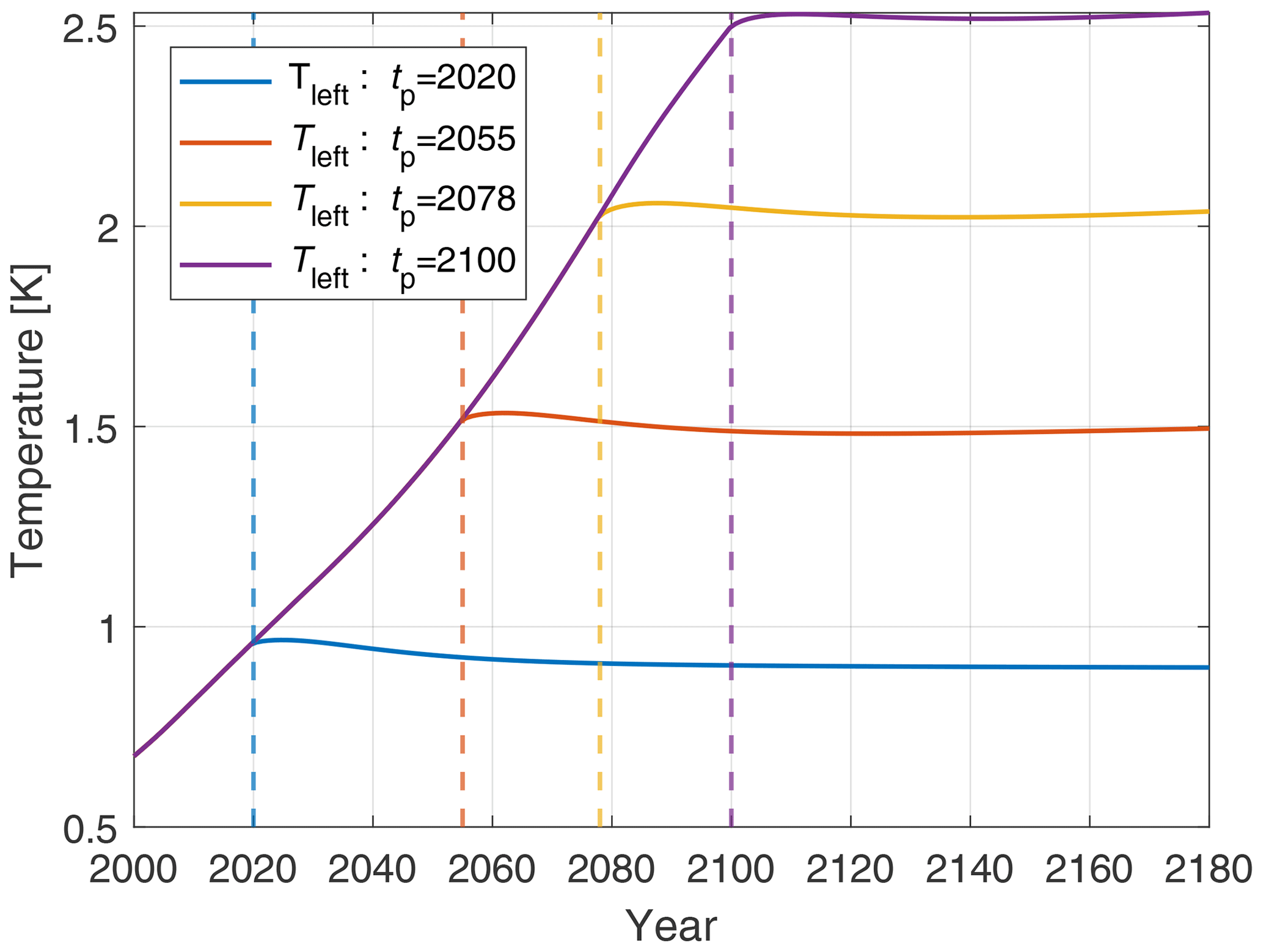
Figure A1 Temperature evolution run up to (RCP6.0 emission scenario) and following the emission cessation at different years t_p. The blue line represents T_left(t), added to Green's integral to compensate for the temperature evolution leftover from prior to the optimization year t₀=2020.