Estimating freshwater flux amplification with ocean tracers via linear response theory

Accurate estimation of changes in the global hydrological cycle over the historical record is important for model evaluation and understanding future trends. Freshwater flux trends cannot be accurately measured directly, so quantification of change often relies on ocean salinity trends. However, anthropogenic forcing has also induced ocean transport change, which imprints on salinity. We find that this ocean transport affects the surface salinity of the saltiest regions (the subtropics) while having little impact on the surface salinity in other parts of the globe. We present a method based on linear response theory which accounts for the regional impact of ocean circulation changes while estimating freshwater fluxes from ocean tracers. Testing on data from the Community Earth System Model large ensemble, we find that our method can recover the true amplification of freshwater fluxes, given thresholded statistical significance values for salinity trends. We apply the method to observations and conclude that from 1975–2019, the hydrological cycle has amplified by 5.04±1.27 % per degree Celsius of surface warming.

1 Introduction

Under anthropogenic forcing, the hydrological cycle is expected to intensify; both global mean precipitation and the pattern of evaporation minus precipitation (E−P) are predicted to amplify (Hegerl et al., 2015). Global mean precipitation is expected to increase at a rate of 2 % °C⁻¹–3 % °C⁻¹, less than the Clausius–Clapeyron rate (7 % °C⁻¹), due to energetic constraints governing tropospheric radiative cooling (Chou and Neelin, 2004; Muller and O'Gorman, 2011; Trenberth, 2011; O'Gorman, 2012; Allan et al., 2014). This 2 % °C⁻¹–3 % °C⁻¹ rate is also predicted by climate models, e.g., the CMIP6 ensemble projects an increase in mean precipitation of 2.1 % °C⁻¹–3.1 % °C⁻¹ in abrupt four times CO₂ experiments (Pendergrass, 2020). However, the amplification rate of E−P patterns, such that wet regions get wetter and dry regions get drier, is more uncertain. While this pattern amplification is linked to the Clausius–Clapeyron relationship, changes in the large scale atmospheric circulation could result in a smaller intensification rate (Held and Soden, 2006), thereby limiting theoretical predictions of the amplification of the E−P pattern. Recent generations of the CMIP model ensembles predict amplification values less than those of Clausius–Clapeyron, but with a large spread. The CMIP5 model ensemble projects an amplification of the E−P pattern of 4.3 ± 2.0 % °C⁻¹ (Skliris et al., 2016). In CMIP6, E−P pattern intensification is estimated at 0.3 %–4.6 %, based on freshwater transport from the subtropics and tropics to polar regions over the period 1970–2014 (Sohail et al., 2022).

Given the gap in theoretical understanding and the spread of amplification in models, an accurate benchmark of E−P pattern change over the historical period is needed. However, due to the difficulty in measuring freshwater flux trends directly, changes both in mean precipitation and the E−P pattern are uncertain over the historical record (Hegerl et al., 2015). Detection of amplified E−P patterns is mostly approached using ocean salinity changes (Douville et al., 2021). This idea of using salinity as a “rain gauge” stems from Wust (1936) who highlighted the similarity between surface salinity and E−P patterns. Recently, studies have used either surface salinity patterns (Durack et al., 2012; Zika et al., 2018) or three-dimensional ocean salinity (e.g., Hosoda et al., 2009; Curry et al., 2003; Helm et al., 2010; Skliris et al., 2014; Cheng et al., 2020; Sohail et al., 2022) to infer changes in surface freshwater fluxes. For the rest of this paper, we refer to the amplification of the E−P pattern (rather than changes in mean precipitation) when referencing change in the hydrological cycle.

Estimates of hydrological cycle change using surface salinity utilize that amplification of the E−P pattern is expected to contribute to salinity pattern amplification whereby areas of the ocean surface that are saltier (or fresher) than average in the climatological mean get saltier (or fresher) (Durack et al., 2012). The AR6 report states that the near-surface salinity contrast between high and low salinity regions has increased by 0.07–0.20 pss (practical salinity scale) from 1950 to 2019 (Fox-Kemper et al., 2021). Durack et al. (2012) estimated amplification of freshwater fluxes by defining a pattern amplification metric as the linear regression between climatological values of a quantity (e.g., surface salinity) and trends of that quantity at the same location. The relationship between the pattern amplification of salinity and of E−P in CMIP3 models was applied to infer E−P changes from surface salinity observations. This empirical relationship between changes in salinity and E−P patterns in models is one way to estimate fluxes from ocean tracers. However, the local change in surface salinity can be affected both by freshwater fluxes and by changes in ocean transport (e.g., Zika et al., 2018). Vinogradova and Ponte (2017) highlighted that local surface salinity is affected by non-negligible effects of isopycnal mixing, diapycnal mixing, and advection. Turner et al. (2022) estimated redistributed salinity, where a redistributed tracer field is defined as the reorganization of the pre-industrial tracer through anomalous transport. They found that redistributed salinity was significant at the surface in some regions, although still smaller than the effect of E−P. Additionally, Sohail et al. (2022) showed that in some regions of the ocean (e.g., the 2 % warmest volume), salinity changes are influenced by both surface fluxes and ocean transport. Finally, recent work shows significant heat redistribution over the historical record (e.g., Winton et al., 2013; Gregory et al., 2016; Bronselaer and Zanna, 2020). These changes in ocean transport suggest an impact of ocean dynamics on local salinity trends. Zika et al. (2018) estimated hydrological cycle amplification utilizing the surface pattern amplification metric from Durack et al. (2012) and accounting for the impact of an idealized surface heat flux on the salinity pattern. Thus, this work accounted for heat flux induced ocean transport changes under the assumption that this redistribution contributes to a linear amplification of the climatological salinity pattern.

Studies linking interior ocean salinity change to surface freshwater fluxes have either examined salinity changes in volumes bounded by depth surfaces (Hosoda et al., 2009; Curry et al., 2003; Skliris et al., 2014; Cheng et al., 2020) or in watermass-based frameworks (Helm et al., 2010; Skliris et al., 2016; Zika et al., 2015; Sohail et al., 2022). Using full-depth salinity negates difficulties with discerning between local changes due to the imprint of fluxes versus ocean transport. However, this approach is limited by reliance on interior salinity data, which have larger uncertainties than the surface due to poor sampling (Durack, 2015; Cheng et al., 2020).

This work presents a novel estimate of E−P pattern amplification over the historical period. We hypothesize (and will test in this paper) that ocean transport change induced by heat fluxes contributes to different regional changes in salinity. We propose a methodology that can account for these local effects of ocean transport when estimating fluxes from tracers. Here, we focus on surface salinity, which is more reliable than full-depth salinity, and on the application of linear response theory (Ruelle, 2009) regionally, thereby relaxing assumptions made in Durack et al. (2012) and Zika et al. (2018). Our method relies on two assumptions, which we will validate: (1) the change in regional ocean tracers under anthropogenic forcing can be expressed as the sum of the effect from freshwater fluxes, heat fluxes, and wind stress change applied separately; and (2) for each component (e.g., freshwater flux forcing), the response of surface tracers is linear with respect to the forcing and therefore linear response theory can be applied.

In this paper, we first introduce the main methodology based on a specific application of linear response theory, in Sect. 2. We then validate and test the method using the Community Earth System Model (CESM) data in Sect. 3. In Sect. 4, we apply the method to observations and estimate freshwater flux changes from 1975 to 2019.

2 Methodology

We propose a method to estimate freshwater fluxes from surface salinity pattern change while accounting for the impact of heat flux or wind stress induced circulation change on salinity. The method is based on a specific application of linear response theory on a few key surface regions. These surface regions are defined as locations with similar salinity, as identified using a Gaussian mixture model (GMM; an unsupervised machine learning algorithm).

2.1 Linear response theory

We start by reviewing linear response theory. Response theory, a generalization of the fluctuation dissipation theorem, can be applied to non-equilibrium and chaotic dynamical systems, such as climate, to predict statistical properties both near and far from equilibrium (Lucarini and Sarno, 2011; Lembo et al., 2020). Following other climate studies (Lucarini and Sarno, 2011; Lembo et al., 2020; Ragone et al., 2016; Torres Mendonça et al., 2021), we use linear response theory from Ruelle (2009) which assumes a dynamical system of the form

$$\begin{array}{}\text{(1)}& {\displaystyle \frac{\mathrm{d}\mathit{x}}{\mathrm{d}t}}=\mathit{A}\left(\mathit{x}\right)+\mathit{B}\left(\mathit{x}\right)f\left(t\right),\end{array}$$

where x(t) is the state vector (e.g., a possibly infinite vector encoding the state of the climate system at time t), A(x) is a vector field representing the system's unperturbed dynamics, B(x) is a vector field representing the pattern of the forcing, and f(t) is the time evolution of the forcing (e.g., anthropogenic emissions).

Consider a given vector of observables, Y(x(t)), which are quantities observed or measured that depend on the state vector of the system. The expectation value of Y(x(t)) can be written as

$$\begin{array}{}\text{(2)}& \langle \mathit{Y}\rangle \left(t\right)=\langle \mathit{Y}{\rangle }_{\mathrm{0}}+\sum _{n=\mathrm{1}}^{\mathrm{\infty }}\langle \mathit{Y}{\rangle }^{\left(n\right)}\left(t\right),\end{array}$$

where 〈Y〉₀ is the expectation value in the unperturbed state and 〈Y〉⁽ⁿ⁾(t) gives the nth order perturbative contribution. Considering only the first order (linear) contribution, the expectation of ΔY(t), the deviation of the observable vector from the unperturbed system, is given by

$$\begin{array}{}\text{(3)}& \langle \mathrm{\Delta }\mathit{Y}\rangle \left(t\right)=\underset{\mathrm{0}}{\overset{t}{\int }}\mathit{\chi }(t-\mathit{\tau })f\left(\mathit{\tau }\right)\mathrm{d}\mathit{\tau }+\mathcal{O}\left(f^{\mathrm{2}}\right),\end{array}$$

where χ(t) is a vector of the Green's functions of the observables. Thus, χ(t) is the response of the system to a Dirac delta function in the same variable as the forcing f(t); if f(t) is anthropogenic CO₂ emissions, then χ(t) is the response to an instantaneous impulse of CO₂. Equation (3) can also be written as

$$\begin{array}{}\text{(4)}& \langle \mathrm{\Delta }\mathit{Y}\rangle \left(t\right)=\underset{\mathrm{0}}{\overset{t}{\int }}\mathit{R}(t-\mathit{\tau }){\displaystyle \frac{\mathrm{d}F}{\mathrm{d}\mathit{\tau }}}\left(\mathit{\tau }\right)\mathrm{d}\mathit{\tau }+\mathcal{O}\left(f^{\mathrm{2}}\right),\end{array}$$

where R(t) is a vector of the observables' responses to a step forcing rather than an impulse forcing (Hasselmann et al., 1993).

2.2 Estimating surface fluxes using linear response theory

In this section, we outline our methodology to infer surface fluxes from regional ocean tracer data by applying response theory.

2.2.1 Dimensionality reduction to characterize salinity pattern

We aim to relate global surface fluxes to the evolving surface salinity pattern. We track pattern evolution using trends in regional salinity, and thus, first find a reduced number of regions that make up the salinity pattern. This dimensionality reduction is performed using a GMM which fits a distribution as the sum of n Gaussians (called mixtures), each with its own mean, standard deviation, and weight. The weights of all the n mixtures sum to 1 (Brunton and Kutz, 2019). Here, we fit a GMM to the climatological surface salinity distribution to decompose the global salinity pattern into regions of similar salinity. Details on the application to data, including the period used to compute climatologies, are in Sect. 3. In practice, we fit the GMM using the sklearn package in Python, which implements the expectation-maximization algorithm (Pedregosa et al., 2011). We make parameter choices of 40 initial conditions and a convergence tolerance of 10⁻³. After fitting, we categorize each point on the ocean surface into a mixture if the climatological salinity of that point is most likely to lie in that particular Gaussian.

GMMs are useful for identifying patterns in oceanographic data (e.g., watermass identification) and can be used as an intermediate between local analysis and domain averaging (Maze et al., 2017; Jones et al., 2019). However, GMMs are sensitive to the number of mixtures. This choice can be guided by criteria such as the Akaike information criterion (AIC) and the Bayesian information criterion (BIC) to balance overfitting with goodness of fit, but it also depends on the scientific question being addressed. We explore the sensitivity to mixture number for our application in Sect. 4.

The dimensionality reduction step allows us to reduce the complexity of the problem as we can characterize the change in the salinity pattern by considering the trends in a few ocean surface regions. We also have avoided imposing that the evolving pattern be a scaled version of the climatological pattern, as each region making up the surface pattern can have a different trend.

2.2.2 Flux estimation using the ensemble mean

As shown in Eq. (4), linear response theory requires the response of observables to a step forcing, R(t). In this proposed framework, the observables are ocean tracers in surface regions found by the GMM in the dimensionality reduction step (see Sect. 2.2.1). Although we expect freshwater fluxes to have the strongest imprint on salinity, we utilize surface temperature as a tracer in the method as an additional constraint.

Here, we aim to separate out the effect of heat flux, freshwater flux, and wind stress change. Thus, we assume that the change in regional ocean tracers under anthropogenic forcing can be written as the sum of the effect due to individual forcing components imposed separately. We apply linear response theory from Eq. (4) to each individual forcing component, resulting in

$$\begin{array}{}\text{(5)}& \begin{array}{rl}\langle \mathrm{\Delta }\mathit{Y}\rangle \left(t\right)=& \underset{\mathrm{0}}{\overset{t}{\int }}{\mathit{R}}^{\text{h}}(t-\mathit{\tau }){\displaystyle \frac{\mathrm{d}{F}^{\text{h}}}{\mathrm{d}\mathit{\tau }}}\left(\mathit{\tau }\right)\mathrm{d}\mathit{\tau }\\ +& \underset{\mathrm{0}}{\overset{t}{\int }}{\mathit{R}}^{\text{w}}(t-\mathit{\tau }){\displaystyle \frac{\mathrm{d}{F}^{\text{w}}}{\mathrm{d}\mathit{\tau }}}\left(\mathit{\tau }\right)\mathrm{d}\mathit{\tau }\\ +& \underset{\mathrm{0}}{\overset{t}{\int }}{\mathit{R}}^{\text{s}}(t-\mathit{\tau }){\displaystyle \frac{\mathrm{d}{F}^{\text{s}}}{\mathrm{d}\mathit{\tau }}}\left(\mathit{\tau }\right)\mathrm{d}\mathit{\tau }.\end{array}\end{array}$$

In Eq. (5), 〈ΔY〉(t) has 2n rows, where each row is a time series of surface salinity and temperature in one of the n mixtures. Temperature and salinity change are normalized in the L² norm such that the scale of change of temperature observables is equal to the scale of change of salinity observables. The tracers are then area-weighted using the area of the GMM region to which they belong. R^h(t), R^w(t), and R^s(t) are also each composed of 2n rows. Each row is a time series of (normalized and area-weighted) temperature and salinity responses to heat flux, freshwater flux, and wind stress step forcings, respectively, in each GMM region. Finally, the terms $\frac{\mathrm{d}{F}^{\text{h}}}{\mathrm{d}t}$, $\frac{\mathrm{d}{F}^{\text{w}}}{\mathrm{d}t}$, and $\frac{\mathrm{d}{F}^{\text{s}}}{\mathrm{d}t}$ are derivatives of the time evolutions of each forcing as a proportion of the strength of the step forcings used for the response functions R^h(t), R^w(t), and R^s(t). For example, if the heat flux response at time t₁ was attributed to a forcing exactly equal to the step forcing, then F^h(t₁)=1.

The system in Eq. (5) is discretized with a time step, Δt, equal to 1 year. We choose this time discretization as it is the shortest time step that smooths over seasonal variability in temperature and salinity data. Thus, the discretized version of Eq. (5) is

$$\begin{array}{}\text{(6)}& \begin{array}{rl}\langle \mathrm{\Delta }\mathit{Y}\rangle \left(t\right)=& \sum _{k=\mathrm{0}}^m{\mathit{R}}^{\text{h}}(m-k){\displaystyle \frac{\mathrm{d}{F}^{\text{h}}}{\mathrm{d}t}}\left(k\right)\\ +& \sum _{k=\mathrm{0}}^m{\mathit{R}}^{\text{w}}(m-k){\displaystyle \frac{\mathrm{d}{F}^{\text{w}}}{\mathrm{d}t}}\left(k\right)\\ +& \sum _{k=\mathrm{0}}^m{\mathit{R}}^{\text{s}}(m-k){\displaystyle \frac{\mathrm{d}{F}^{\text{s}}}{\mathrm{d}t}}\left(k\right).\end{array}\end{array}$$

Here, the known variables are the response functions and the ensemble-averaged observable vector anomaly, 〈ΔY〉(t). At each time step, we solve for the unknowns $\frac{\mathrm{d}{F}^{\text{h}}}{\mathrm{d}t}$, $\frac{\mathrm{d}{F}^{\text{w}}}{\mathrm{d}t}$, and $\frac{\mathrm{d}{F}^{\text{s}}}{\mathrm{d}t}$ using the normal equations (see Appendix A for details). We then numerically integrate $\frac{\mathrm{d}{F}^{\text{h}}}{\mathrm{d}t}$, $\frac{\mathrm{d}{F}^{\text{w}}}{\mathrm{d}t}$, and $\frac{\mathrm{d}{F}^{\text{s}}}{\mathrm{d}t}$ in time to obtain time series F^w(t),F^h(t), and F^s(t). In Sect. 3, we describe the data that we use as response functions to apply this method in practice.

2.2.3 Flux estimation using individual realizations

Crucially, Eq. (5) holds for the expectation of the change in observables, 〈ΔY〉(t). For applications to climate, this implies that it holds for the ensemble average, rather than individual realizations such as observations. Thus, we create an artificial ensemble for individual realizations by detrending the data, applying block bootstrapping, and adding the trend back following the methodology from McKinnon et al. (2017). For the block bootstrapping, we use a block size of 2 years, which is larger than the autocorrelation time scale of the observables. We test the dependence of results on block size in Sect. 4.

We first apply linear response theory to an individual ensemble member (a single realization) as

$$\begin{array}{}\text{(7)}& \begin{array}{rl}\mathrm{\Delta }{\mathit{Y}}_{\mathit{i}}\left(t\right)=& \underset{\mathrm{0}}{\overset{t}{\int }}{\mathit{R}}^{\text{h}}(t-\mathit{\tau }){\displaystyle \frac{\mathrm{d}{F}_i^{\text{h}}}{\mathrm{d}\mathit{\tau }}}\mathrm{d}\mathit{\tau }+\underset{\mathrm{0}}{\overset{t}{\int }}{\mathit{R}}^{\text{w}}(t-\mathit{\tau }){\displaystyle \frac{\mathrm{d}{F}_i^{\text{w}}}{\mathrm{d}\mathit{\tau }}}\mathrm{d}\mathit{\tau }\\ +& \underset{\mathrm{0}}{\overset{t}{\int }}{\mathit{R}}^{\text{s}}(t-\mathit{\tau }){\displaystyle \frac{\mathrm{d}{F}_i^{\text{s}}}{\mathrm{d}\mathit{\tau }}}\mathrm{d}\mathit{\tau }+\mathit{\eta }\left(t\right),\end{array}\end{array}$$

where ΔY_i(t) is the change in the observable vector for the ith individual ensemble member. Here, as the observables are not ensemble-averaged, the equation includes an unknown noise term, η(t). The noise term has 2n rows, where each row corresponds to an observable (salinity or temperature in one of the n mixtures) (e.g., Torres Mendonça et al., 2021). We discretize Eq. (7) in the same way as Eq. (5), and

$$\begin{array}{}\text{(8)}& \begin{array}{rl}\mathrm{\Delta }{\mathit{Y}}_i\left(t\right)=& \sum _{k=\mathrm{0}}^m{\mathit{R}}^{\text{h}}(m-k){\displaystyle \frac{\mathrm{d}{F}_i^{\text{h}}}{\mathrm{d}t}}\left(k\right)\\ +& \sum _{k=\mathrm{0}}^m{\mathit{R}}^{\text{w}}(m-k){\displaystyle \frac{\mathrm{d}{F}_i^{\text{w}}}{\mathrm{d}t}}\left(k\right)\\ +& \sum _{k=\mathrm{0}}^m{\mathit{R}}^{\text{s}}(m-k){\displaystyle \frac{\mathrm{d}{F}_i^{\text{s}}}{\mathrm{d}t}}\left(k\right)+\mathit{\eta }\left(t\right)\end{array}\end{array}$$

follows. The averaged version of Eq. (7) is

$$\begin{array}{}\text{(9)}& \begin{array}{rl}& \langle \mathrm{\Delta }\mathbf{Y}\left(t\right)\rangle \\ & =\langle \underset{\mathrm{0}}{\overset{t}{\int }}{\mathit{R}}^{\text{h}}(t-\mathit{\tau }){\displaystyle \frac{\mathrm{d}{F}_i^{\text{h}}}{\mathrm{d}\mathit{\tau }}}\mathrm{d}\mathit{\tau }+\underset{\mathrm{0}}{\overset{t}{\int }}{\mathit{R}}^{\text{w}}(t-\mathit{\tau }){\displaystyle \frac{\mathrm{d}{F}_i^{\text{w}}}{\mathrm{d}\mathit{\tau }}}\mathrm{d}\mathit{\tau }\\ & +\underset{\mathrm{0}}{\overset{t}{\int }}{\mathit{R}}^{\text{s}}(t-\mathit{\tau }){\displaystyle \frac{\mathrm{d}{F}_i^{\text{s}}}{\mathrm{d}\mathit{\tau }}}\mathrm{d}\mathit{\tau }+\mathit{\eta }\left(t\right)\rangle \\ & =〈\underset{\mathrm{0}}{\overset{t}{\int }}{\mathit{R}}^{\text{h}}(t-\mathit{\tau }){\displaystyle \frac{\mathrm{d}{F}_i^{\text{h}}}{\mathrm{d}\mathit{\tau }}}\mathrm{d}\mathit{\tau }〉+〈\underset{\mathrm{0}}{\overset{t}{\int }}{\mathit{R}}^{\text{w}}(t-\mathit{\tau }){\displaystyle \frac{\mathrm{d}{F}_i^{\text{w}}}{\mathrm{d}\mathit{\tau }}}\mathrm{d}\mathit{\tau }〉\\ & +〈\underset{\mathrm{0}}{\overset{t}{\int }}{\mathit{R}}^{\text{s}}(t-\mathit{\tau }){\displaystyle \frac{\mathrm{d}{F}_i^{\text{s}}}{\mathrm{d}\mathit{\tau }}}\mathrm{d}\mathit{\tau }〉,\end{array}\end{array}$$

where 〈.〉 is the ensemble average over all ensemble members and 〈η(t)〉=0. We assume that Eqs. (5) and (9) are approximately equivalent; in other words, we assume that $[\langle \frac{\mathrm{d}{F}_i^{\text{h}}}{\mathrm{d}t}\rangle ,\langle \frac{\mathrm{d}{F}_i^{\text{w}}}{\mathrm{d}t}\rangle ,\langle \frac{\mathrm{d}{F}_i^{\text{s}}}{\mathrm{d}t}\rangle ]\approx [\frac{\mathrm{d}{F}^{\text{h}}}{\mathrm{d}t},\frac{\mathrm{d}{F}^{\text{w}}}{\mathrm{d}t},\frac{\mathrm{d}{F}^{\text{s}}}{\mathrm{d}t}]$.

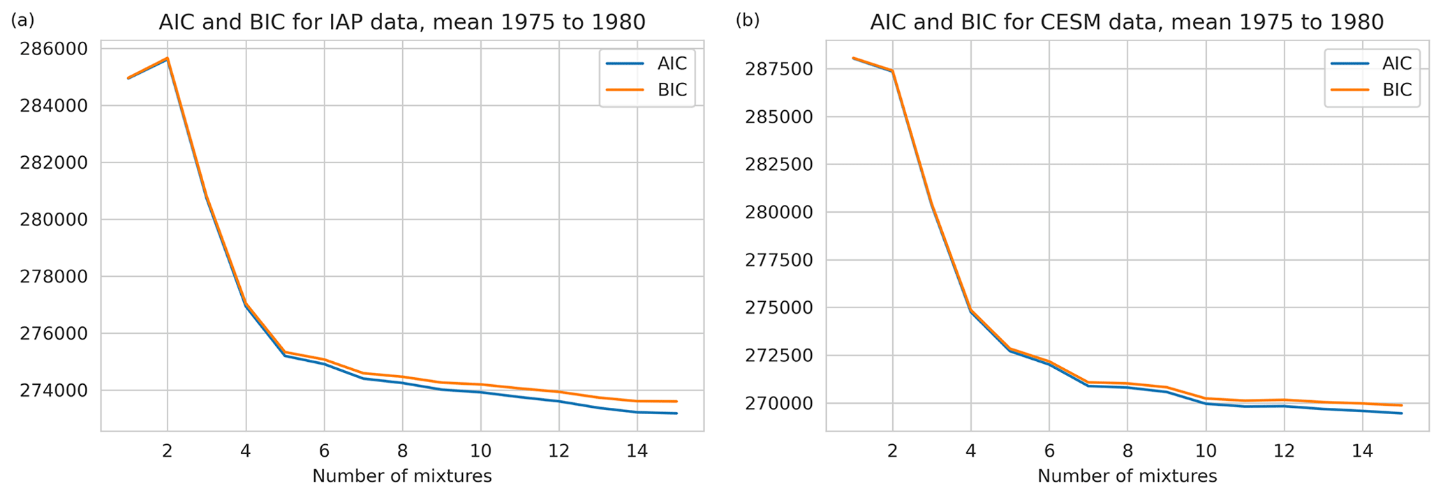
Figure 1 The AIC and BIC versus number of mixtures. Panel (a) uses the Institute of Atmospheric Physics (IAP) surface salinity distribution south of 65° N over the period 1975 to 1980, while (b) uses the CESM ensemble mean surface salinity distribution over the same region and time period.

For each member of an artificial ensemble created by block bootstrapping, we solve Eq. (8) for $[\frac{\mathrm{d}{F}_i^{\text{h}}}{\mathrm{d}t},\frac{\mathrm{d}{F}_i^{\text{w}}}{\mathrm{d}t},\frac{\mathrm{d}{F}_i^{\text{s}}}{\mathrm{d}t}]$, ignoring the effect of η(t). We estimate the mean $[\frac{\mathrm{d}{F}^{\text{h}}}{\mathrm{d}t},\frac{\mathrm{d}{F}^{\text{w}}}{\mathrm{d}t},\frac{\mathrm{d}{F}^{\text{s}}}{\mathrm{d}t}]$ with associated error by taking the average and standard deviation across artificial ensemble members of $[\frac{\mathrm{d}{F}_i^{\text{h}}}{\mathrm{d}t},\frac{\mathrm{d}{F}_i^{\text{w}}}{\mathrm{d}t},\frac{\mathrm{d}{F}_i^{\text{s}}}{\mathrm{d}t}]$ as Eq. (9) implies.

Throughout the next two sections (Sects. 3 and 4), we introduce data products for the application of the method in practice, for validation, and for rescaling of our freshwater flux change estimate in terms of a percentage change of the hydrological cycle per degree Celsius. These data will be explained in text in detail as they are introduced; however, for convenience a summary is provided in Table 1.

(Gregory et al., 2016; Todd et al., 2020)(Kay et al., 2015)(Cheng and Zhu, 2016; Cheng et al., 2020)(Forget et al., 2015; ECCO Consortium et al., 2021)(Lenssen et al., 2019; GISTEMP Team, 2023)

Table 1 A summary of data products used throughout the paper for application of the method, validation, and rescaling our final result as a percentage change of the hydrological cycle per degree Celsius. The data listed here are described in more detail in Sects. 3 and 4.

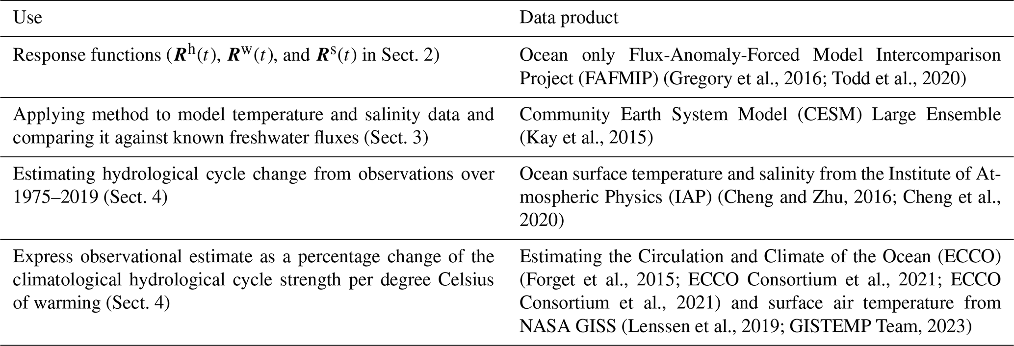
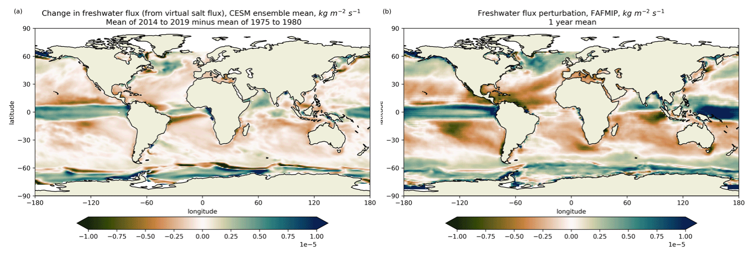
Figure 2 Change in ensemble mean CESM freshwater fluxes over 1975–2019 (a) and the annual mean freshwater flux perturbation map from FAFMIP (b) (Gregory et al., 2016; Todd et al., 2020). The FAFMIP map is N(x,y) in Eq. (10). Here, fluxes are defined such that positive is downward, from the atmosphere into the ocean.

3 Validation of surface flux estimates from linear response theory in CESM

In this section, we use 34 members of the CESM large ensemble (ensemble members 001–035) over the period 1975–2019 to develop, test, and validate the methodology of surface flux estimation. The forcing used in the simulation is historical until 2005 and then RCP8.5 onwards (Kay et al., 2015). The CESM ensemble mean freshwater flux change over the period considered is shown in Fig. 2a.

3.1 Extracting observables and response functions

To select the main regions defining the salinity pattern (and our observables), we fit a GMM to the surface salinity distribution of the CESM ensemble mean over 1975–1980 (see Sect. 2.2.1). We include all points south of 65° N; the Arctic is excluded for simplicity due to its small size and to remove the potential effect of sea ice melt on salinity. Using the elbow metric on the AIC and BIC (Fig. 1b), the possible number of mixtures is between 5 and 7. In the subsequent analysis, we use six mixtures and show in Sect. 4 the lack of sensitivity to that choice. The GMM fit to the CESM ensemble mean data is shown in Fig. 3a and b.

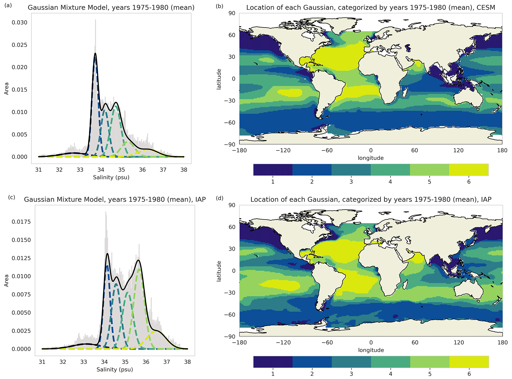
Figure 3 GMMs fit to the mean surface salinity distribution (a, c) and location of mixtures based on these models (b, d). The top row (a, b) uses surface salinity data from the CESM large ensemble with a mean across 34 members of the ensemble and over the period 1975–1980 (Kay et al., 2015). The bottom row (c, d) uses surface salinity data from the IAP (Cheng et al., 2020) with a mean over the period 1975–1980.

To estimate the response functions, we introduce data from the ocean-only Flux-Anomaly-Forced Model Intercomparison Project (FAFMIP). FAFMIP will be used to extract R^h(t), R^w(t), and R^s(t) as defined in Sect. 2. In the ocean FAFMIP experiments, heat flux, freshwater flux, and wind stress perturbations associated with CO₂ doubling are imposed separately on ocean models (Gregory et al., 2016; Todd et al., 2020). For example, the FAFMIP freshwater flux perturbation imposed as a step function is shown in Fig. 2b. Data from FAFMIP is well suited to our method because forcings are imposed both as step functions and as individual components (see Eqs. 4 and 5). Thus, the salinity and temperature responses to FAFMIP perturbations are used in our method as the response functions (R^h(t), R^w(t), and R^s(t)) in Eq. (5). The equation is set up using response functions derived from each FAFMIP ocean model and solved for $\frac{\mathrm{d}{F}^{\text{h}}}{\mathrm{d}t},\frac{\mathrm{d}{F}^{\text{w}}}{\mathrm{d}t},\text{and}\frac{\mathrm{d}{F}^{\text{s}}}{\mathrm{d}t}$ terms. We then take the mean of the resultant $\frac{\mathrm{d}{F}^{\text{h}}}{\mathrm{d}t},\frac{\mathrm{d}{F}^{\text{w}}}{\mathrm{d}t},\text{and}\frac{\mathrm{d}{F}^{\text{s}}}{\mathrm{d}t}$ values across ocean models (ACCESS-OM2, HadOM3, and MITgcm). There is a 15-year relatively fast response of the ocean state after applying the FAFMIP abrupt forcing, before a slow and steady linear response to the forcing which we are trying to capture. Therefore, we truncate the time series of the response functions such that R^h(0), R^w(0), and R^s(0) are taken to be between 15 and 20 years after the forcing is applied. Thus, in practice, the linear response theory expressions (Eqs. 6 and 8) are solved for each adjustment time (between 15 and 20 years) and the mean is taken.

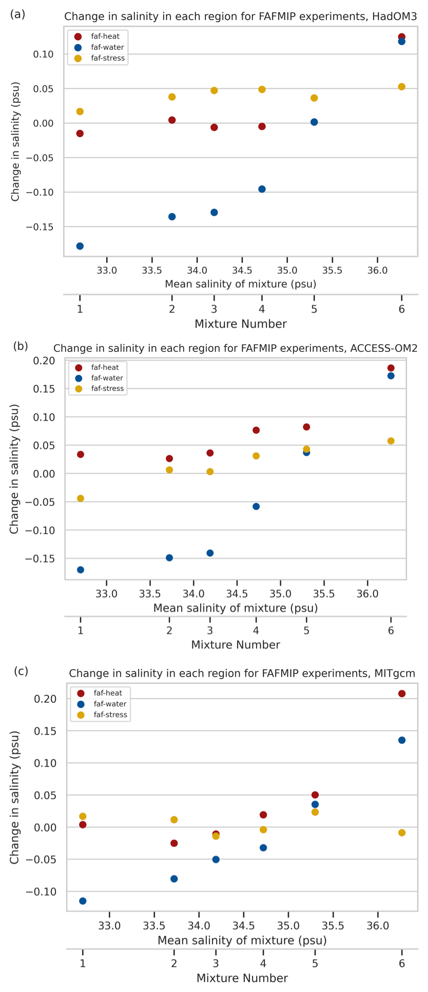
Figure 4 The change in surface salinity in each region from the GMM applied to the CESM ensemble mean data (see Fig. 3b) for each individual forcing experiment. The heat flux experiment (faf-heat) is shown in red, freshwater flux (faf-water) in blue, and wind stress perturbation (faf-stress) in yellow. The response is defined as the difference between the last decade of a forced run and the last decade of the control run. Panels (a)–(c) show the results for ocean models HadOM3, ACCESS-OM2, and MITgcm, respectively.

3.2 Impact of ocean transport and linearity of forcings on surface salinity

At the end of Sect. 1, we hypothesized that global heat fluxes affect regional surface salinity differently. Here, we validate this hypothesis by examining the effect of the FAFMIP step forcings – heat flux, freshwater flux, and wind stress change – on surface salinity in GMM regions based on CESM data. The CESM regions (Fig. 3a and b) are used to illustrate the FAFMIP response functions here; however, when applying the full estimation method on a different dataset of interest, the locations of each response function change slightly according to the GMM fit for that dataset. Figure 4 shows the change in each mixture region between the last decade of a forcing experiment and the last decade of control, with each panel showing results for a different FAFMIP ocean model. We find that the freshwater flux forcing makes fresher (or saltier) regions fresher (or saltier) with a nearly linear scaling of change relative to the region's climatological salinity. The heat flux perturbation tends to make saltier regions (mixtures 5 and 6) saltier with little effect in other regions. This means that much of the imprint of heat flux induced circulation change on salinity is in the subtropics. The wind stress change has little effect on the salinity pattern. Figure S4 in the Supplement shows plots comparable to Fig. 4 for surface temperature, but we focus on salinity here as it is the primary tracer affected by freshwater fluxes. For ease of visualization, we also show the change in surface salinity in each FAFMIP experiment and for each ocean model in the CESM mixture regions displayed on maps in Fig. S1 in the Supplement. We confirm that circulation changes, induced by heat fluxes, are regional and imprint on surface salinity with a different spatial pattern than freshwater fluxes. Thus, our methodology, which uses regional tracer changes, can account for the distinct effects of heat fluxes and freshwater fluxes when inferring surface freshwater flux changes.

We invoke two different linearity assumptions in our method. The first assumption of linearity in the methodology is that regional ocean salinity and temperature changes under anthropogenic forcing can be separated into the sum of the effect from freshwater fluxes, heat fluxes, and wind stress change imposed separately. As above, we evaluate this using the effect of FAFMIP step forcings on ocean regions defined by a GMM fit to the CESM ensemble mean salinity distribution (mixture locations in Fig. 3b). Figure 5 compares the change in salinity (5a) and temperature (5b) due to separate imposition of forcings (“faf-stress + faf-water + faf-heat”) and due to forcings applied at once (“faf-all”). We examine agreement by finding the L² norm of the response in the six regions due to forcings imposed individually divided by the L² norm of the response from the combined forcing. These values for surface salinity are 0.916 for MITgcm, 0.959 for ACCESS-OM2, and 1.340 for HadOM3. For surface temperature, these values are 0.974, 0.962, and 1.118. We see good agreement between the sum of individual forcings and forcings applied together. A notable exception is the sixth mixture for the HadOM3 model where there is a non-linear response. Overall, the agreement is sufficiently close to use the linearity approximation, but the disagreement in the sixth mixture for HadOM3 is a caveat of this work.

The second assumption of linearity in the method is that linear response theory holds, i.e., that the change in observables is linear with respect to the forcing strength. In particular, we assume that this holds as in Eq. (5) where linear response theory is applied to individual forcing components. The available data where individual forcing components are imposed on ocean models come from FAFMIP; however, the FAFMIP experiments impose perturbations only as step forcings, so we cannot directly evaluate linearity with respect to forcing strength. Instead, in the next subsections, we validate the full methodology by testing if the true freshwater fluxes from model data can be recovered via our method using only surface salinity and temperature time series.

3.3 Estimating surface flux amplification from CESM ensemble mean data

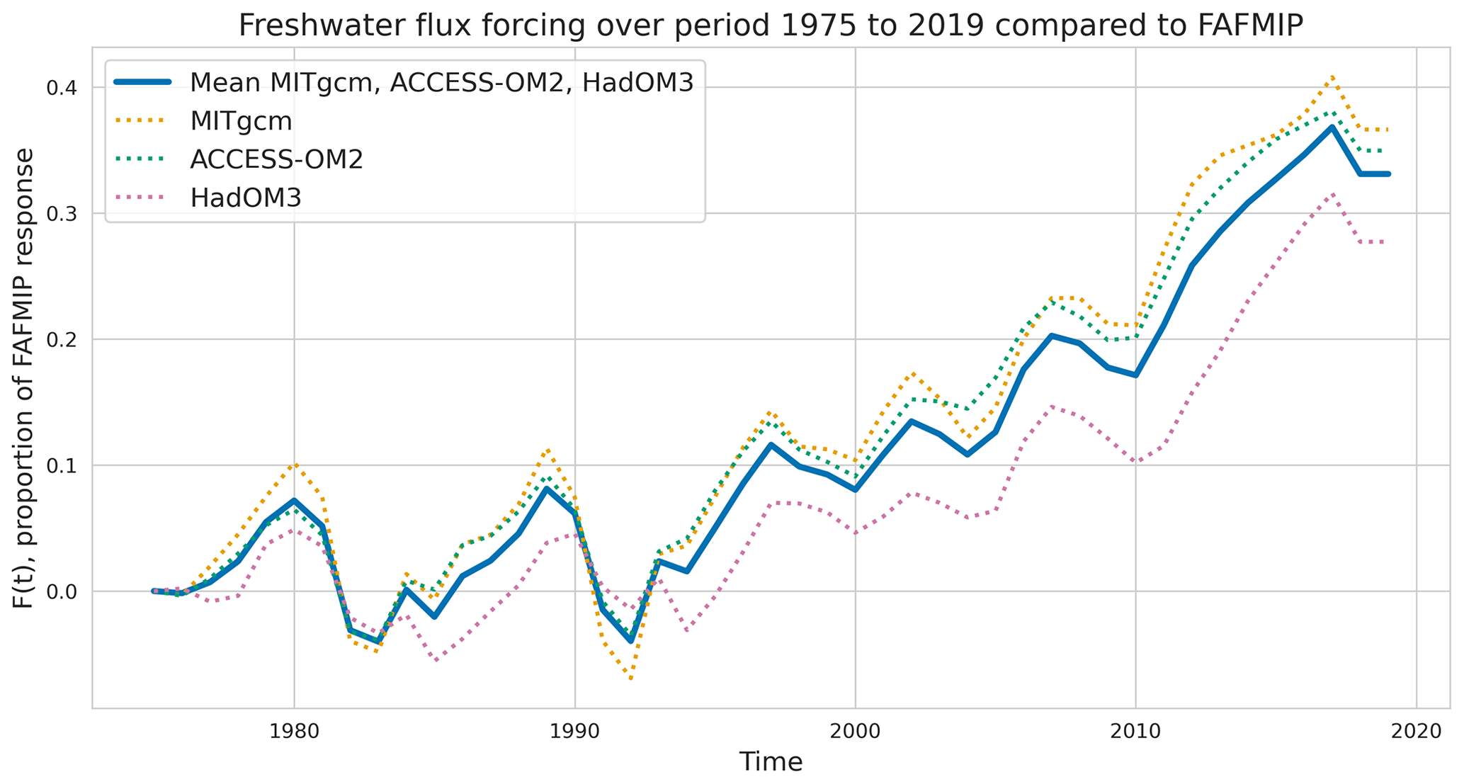
We test the method on the CESM ensemble mean over the period 1975–2019. We apply Eq. (6) where each row of 〈ΔY〉(t) is a time series of (normalized and area-weighted) salinity and temperature in each GMM region from the ensemble mean data. The non-normalized or area-weighted versions of the observables are plotted in Fig. 6. We solve Eq. (6) for the unknown time series of each forcing as a proportion of the step function strength (see Fig. 7 for F^w(t)). To estimate the trend and associated error in F^w(t) (and all other time series throughout the paper), we proceed as follows:

1. Fit a linear trend to the relevant time series (e.g., F^w(t)).

2. Block bootstrap around this trend with blocks of size 2 years to account for internal variability.

3. Refit linear trends to each block bootstrapped time series (totaling 3000 time series).

4. Estimate the mixture distribution for the trends of the 3000 time series.

5. Calculate the mean and standard deviation of the mixture distribution (see Appendix B).

6. Compute the change in the time series (F^w(t)) by multiplying the mean and standard deviation of the trend by the length of the series (here, 45 years).

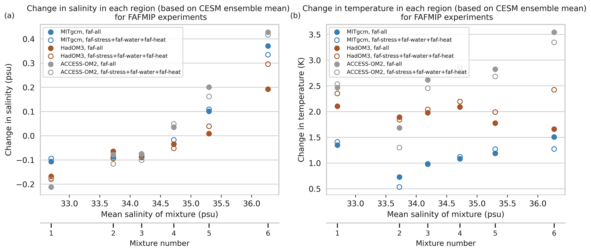
Figure 5 Comparison of the surface salinity response (a) and surface temperature response (b) in each region between two cases: the sum of the response when forcings are applied individually (faf-stress + faf-water + faf-heat) and the response to all forcings applied at once (faf-all). The response is defined as the difference between the last decade of a forced run and the last decade of the control run. The response is largely linear with the exception of the sixth mixture for the HadOM3 model.

We could have instead taken the mean and standard deviation across the aggregate (block bootstrapped) time series by ignoring the error in each refit trend, but this procedure accounts for less error. Using this method on F^w(t) (Fig. 7), we find that the change in freshwater fluxes is 0.3515±0.0432 times the FAFMIP step forcing.

For comparison, we quantify the true response of E−P pattern change by finding the change in the model's freshwater fluxes over both precipitation and evaporation dominated regions. We separately integrate the annual mean freshwater fluxes over the region where the FAFMIP perturbation is positive (precipitation dominated) or negative (evaporation dominated) and then scale by the magnitude of the FAFMIP pattern calculated in the same way. We define the precipitation or evaporation dominated regions using the FAFMIP perturbation because the linear response theory method finds a scaling of this pattern. The target metric is written as

$$\begin{array}{}\text{(10)}& P\left(t\right)={\displaystyle \frac{{\int }_{{\mathrm{\Omega }}_{-}}\mathbf{C}(x,y,t)\mathrm{d}A+{\int }_{{\mathrm{\Omega }}_{+}}\mathbf{C}(x,y,t)\mathrm{d}A}{{\int }_{{\mathrm{\Omega }}_{-}}\mathbf{N}(x,y)\mathrm{d}A+{\int }_{{\mathrm{\Omega }}_{+}}\mathbf{N}(x,y)\mathrm{d}A}},\end{array}$$

where $\mathbf{C}(x,y,t)$ is the freshwater flux pattern from CESM at time t, N(x,y) is the FAFMIP freshwater perturbation pattern (see Fig. 2b), and Ω₋ and Ω₊ are regions where N(x,y) is negative and positive, respectively.

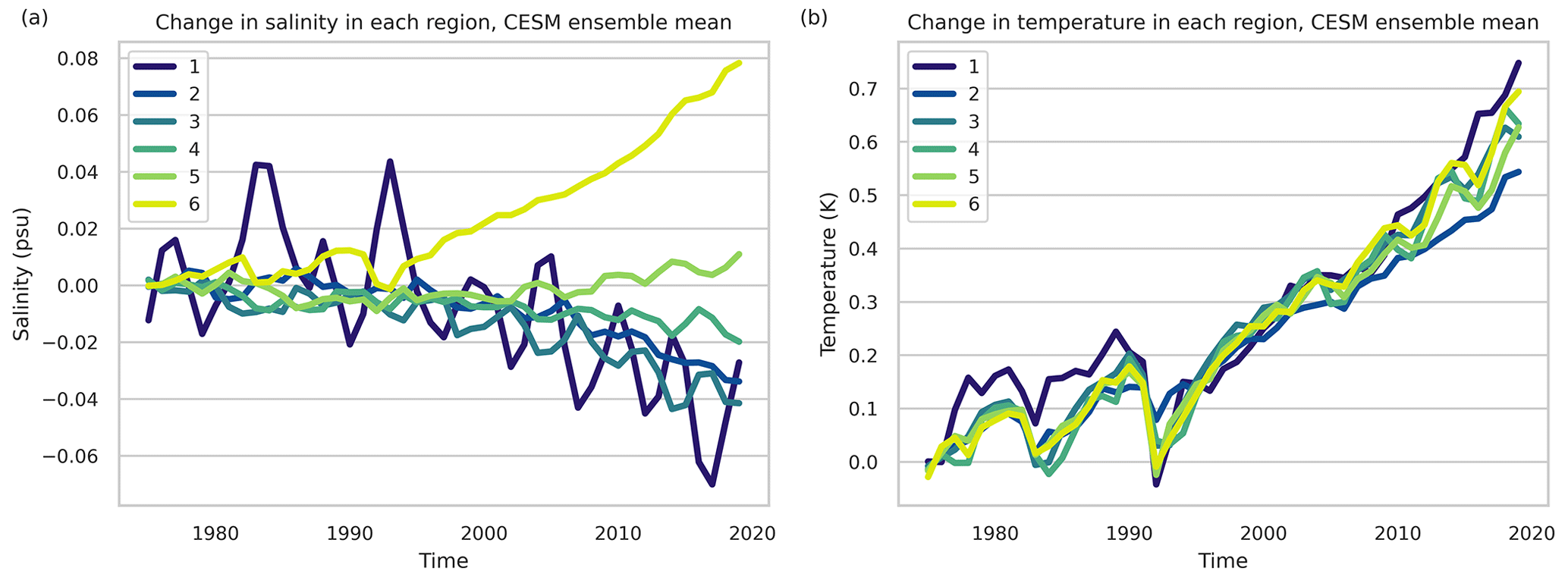
Figure 6 The change in surface salinity (a) and surface temperature (b) in each region from CESM ensemble data over the period 1975–2019. Here, the data are an ensemble mean over 34 members and the anomaly is taken from the mean of the first 2 years. The locations of the mixtures are shown in Fig. 3b.

We account for internal variability in P(t) using block bootstrapping on the time series (Fig. 8) with 2-year blocks and 3000 members (McKinnon et al., 2017). We quantify the change in P(t) using the same process as for F^w(t) above, by refitting new linear trends to each time series created by block bootstrapping and then taking the mean and standard deviation across these. We find that the true change in freshwater fluxes for the CESM ensemble mean is 0.4114±0.0602 times the FAFMIP perturbation. Thus, the result of 0.3515±0.0432 from our method is within error bounds of the truth.

Figure 7 F^w(t) found by solving Eq. (6), where 〈ΔY〉(t) is regional salinity and temperature from the CESM ensemble mean over the period 1975–2019.

3.4 Estimating surface flux amplification from individual ensemble members of CESM

We test the application of the method on individual CESM ensemble members. For this application, the dimensionality reduction step is done for each member by fitting a GMM to the salinity distribution of the individual realization. This results in region categorization analogous to Fig. 3b for each individual member. We create an artificial ensemble around each member. For the ith (artificial) member, we solve Eq. (8) for $[\frac{\mathrm{d}{F}_i^{\text{h}}}{\mathrm{d}t},\frac{\mathrm{d}{F}_i^{\text{w}}}{\mathrm{d}t},\frac{\mathrm{d}{F}_i^{\text{s}}}{\mathrm{d}t}]$. We then quantify the change in each $F_i^{\text{w}}\left(t\right)$ by fitting a linear trend to the time series. We take the mean and standard deviation across all artificial ensemble members, as explained in Appendix B, and find the freshwater flux change with error (see Sect. 2.2.3).

Applying this methodology, we find that the method does not capture the true response for all individual CESM members (see Fig. S5). However, while the CESM members have significant temperature trends over the historical period, many members have insignificant (linear) salinity trends due to variability. In fact, none of the members have all regional linear trends significant at the p<0.05 level. We impose significance criteria by requiring that regions with strong trends across ensemble members, regions 2 and 6, have p<0.05. We require that other regions' trends have p<0.18, i.e., they are insignificant but the internal variability to signal ratio is capped. We exclude restrictions on region 4, as for most members it has a large amount of internal variability but does not affect the result, likely because of its small size. We find six members which meet these statistical significance criteria. For these members, the freshwater flux amplification found by the linear response theory method is plotted in Fig. 9 and compared against the true amplification, determined by the change in Eq. (10).

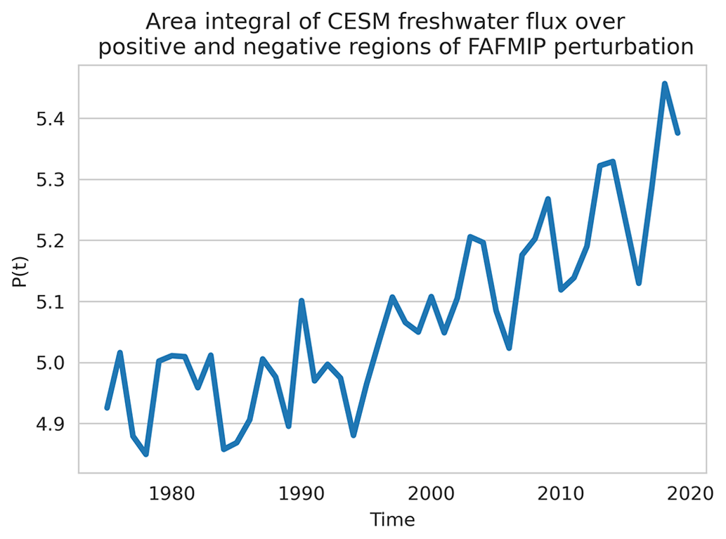
Figure 8 P(t), the target truth metric, as defined in Eq. (10) over the period 1975–2019 for CESM ensemble mean data.

Thus, we find that the method, as outlined in Sect. 2, can capture the true freshwater amplification for individual members provided that the salinity trends meet certain significance criteria. However, our estimate captures less of the amplification uncertainty than the target metric; thus, we propose interpreting the error bars from our method as a lower bound on error. It is sensible that we need significance criteria on salinity trends, as members not meeting them have observables (salinity) dominated by internal variability rather than forced response. This same process is tested in Fig. S6 in the Supplement over the period 2011–2055 where salinity trends are stronger and thus most members reach the significance criteria. In that case, we recover the true result for 90.3 % of members.

4 Estimating freshwater fluxes from observations

In this section, we apply our methodology (outlined in Sects. 2 and 3) to the Institute of Atmospheric Physics (IAP) dataset over the period 1975–2019 (Cheng and Zhu, 2016; Cheng et al., 2020). We focus on the IAP data, as other available observational datasets are either limited in time or have salinity trend biases. In particular, the dataset following Ishii et al. (2005) ends in 2012, while EN4 data (Good et al., 2013) have salinity biases compared with other data. These biases, for example, lead to freshwater flux estimates different from when using other data products in Sohail et al. (2022) (see their Fig. 3).

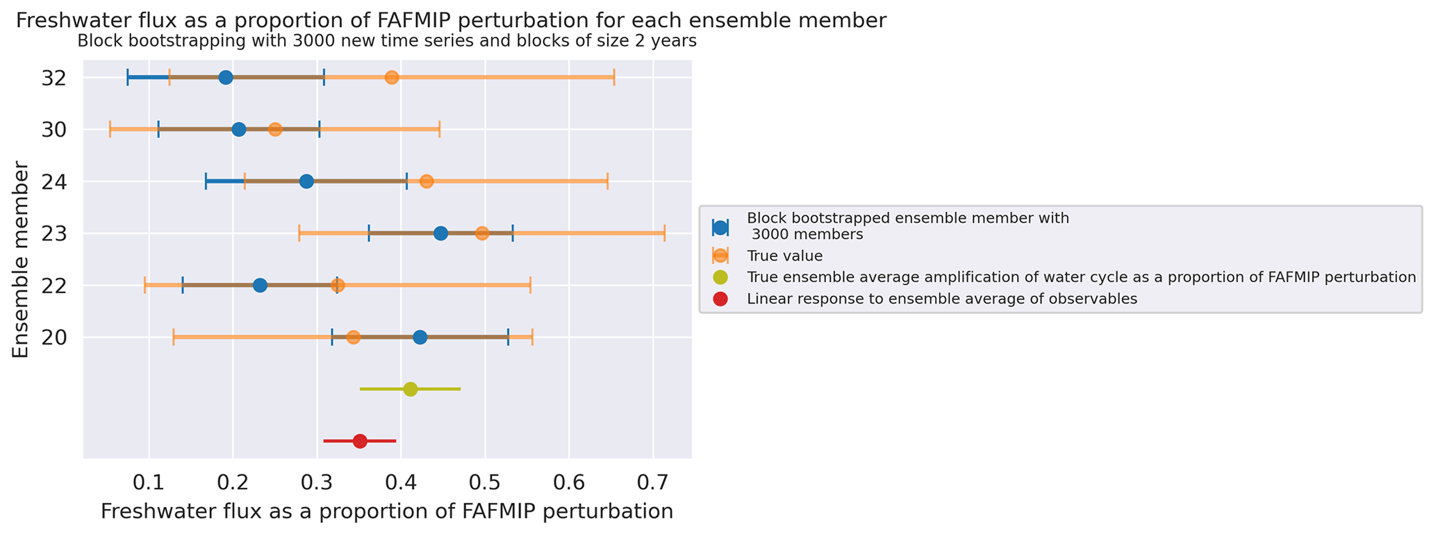
Figure 9 Freshwater flux responses for CESM ensemble members following methodology described in text (blue) compared with truth from E−P model fields (orange). Here, we plot only members which met the salinity trend significance criteria defined in the text. For members meeting the significance criteria, the true amplification of freshwater fluxes is captured within the error bars. The tests on all ensemble members are available in Fig. S5.

Based on AIC and BIC, we use six mixtures for the GMM as a representative choice in the range indicated by the elbow metric (see Fig. 1a) when performing the dimensionality reduction step of the method. The change in temperature and salinity in each region as found by the GMM (see Fig. 3c and d) are shown in Fig. 10. Following the steps from Sect. 3.1, we define the response functions R^h(t), R^w(t), and R^s(t) from the response of salinity and temperature in the FAFMIP experiments in each of these GMM regions defined on the IAP salinity. We then create an artificial ensemble around the original IAP data as required to apply the methodology to a single realization. We find that the observations meet the salinity trend significance criteria outlined in Sect. 3 by a large margin. The p values of linear salinity trends are $\mathrm{6.33}\times {\mathrm{10}}^{-\mathrm{2}}$, $\mathrm{7.55}\times {\mathrm{10}}^{-\mathrm{9}}$, $\mathrm{1.90}\times {\mathrm{10}}^{-\mathrm{3}}$, $\mathrm{6.34}\times {\mathrm{10}}^{-\mathrm{2}}$, $\mathrm{7.75}\times {\mathrm{10}}^{-\mathrm{6}}$, and $\mathrm{3.47}\times {\mathrm{10}}^{-\mathrm{27}}$ for each region, respectively. Thus, the significance criteria based on testing on the CESM large ensemble are met, and the full methodology should recover the true freshwater flux amplification.

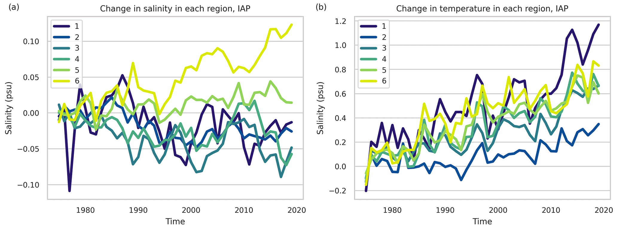
Figure 10 The change in surface salinity (a) and surface temperature (b) in each region from the IAP data over the period 1975–2019. Here, the change is taken from the mean of the first 2 years. The locations of the mixtures are shown in Fig. 3d.

From 1975 to 2019, we find that the freshwater flux response was 0.3278±0.0828 times the FAFMIP perturbation. This value is insensitive to choices made in the methodology including the number of mixtures used in the GMM and choices made in the block bootstrapping step. Table 2 shows the resultant estimate if the methodology had instead been carried through with five or seven mixtures. We also find the estimate is insensitive to block size (Fig. D1) and to the number of artificial ensemble members created (Fig. D2) used in the block bootstrapping step. Thus, the method robustly estimates freshwater fluxes from observational data.

We also note that the hypotheses and assumptions motivating and utilized in the method as tested in Sect. 3 similarly hold for the IAP data. Figures 4 and 5, which used the GMM regions from CESM, have equivalents using GMM regions from the IAP in Figs. S2 and S3.

Our estimate is expressed as a scaling of the FAFMIP perturbation. We now convert it to a percentage change of the climatological hydrological cycle to facilitate comparison with previous studies. This conversion introduces more error into the estimate, requiring scaling the result by other datasets. Here, we use mean freshwater fluxes from the Estimating the Circulation and Climate of the Ocean (ECCO) state estimate as the climatological hydrological cycle strength (see Appendix C) (Forget et al., 2015; ECCO Consortium et al., 2021). We find that our estimate as a proportion of the FAFMIP perturbation is equivalent to hydrological cycle amplification of 4.402±1.112 %. We can also express this as a percentage change per degree Celsius change in surface air temperature. We estimate the change in surface air temperature from NASA GISS data (Lenssen et al., 2019; GISTEMP Team, 2023) by taking the linear trend over 1975 to 2019. Scaling by the surface temperature change, we find an amplification of 5.036±1.272% °C⁻¹ (Fig. 11).

Although we focus on freshwater fluxes, our methodology also finds scalings of the other FAFMIP forcings. From the IAP data, we find a heat flux change of 0.4252±0.0934 times the FAFMIP perturbation. Integrating the FAFMIP heat flux forcing south of 65° N, we find a heat flux increase over 1975–2019 of 0.5938±0.1305 W m⁻². This is within error bounds of other estimates. The AR6 reports a heat flux increase of 0.52±0.15 W m⁻² over 1971–2018 (Gulev et al., 2021), while Cheng et al. (2022) found 0.44±0.08 W m⁻² over the same period.

Table 2 The response as a proportion of the FAFMIP freshwater flux perturbation using different numbers of mixtures in the GMM. Here, the method is applied to the IAP data over the period 1975–2019.

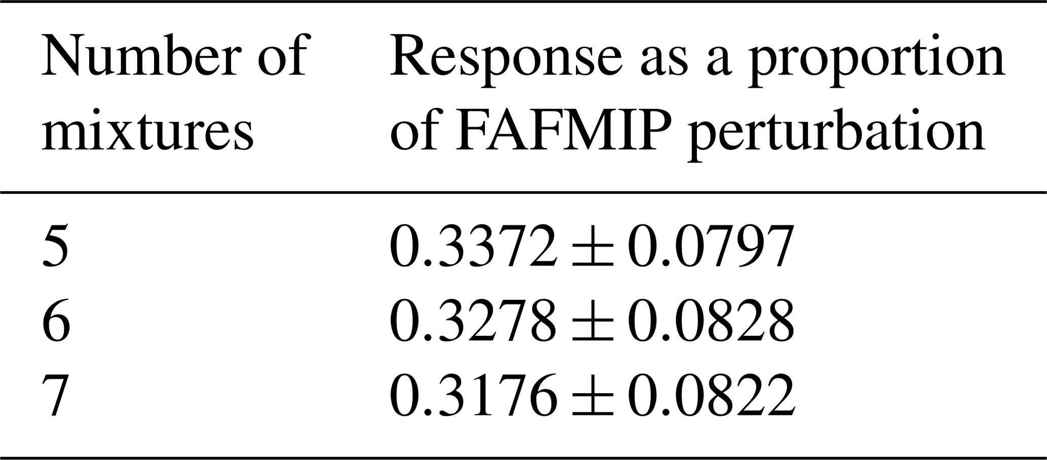
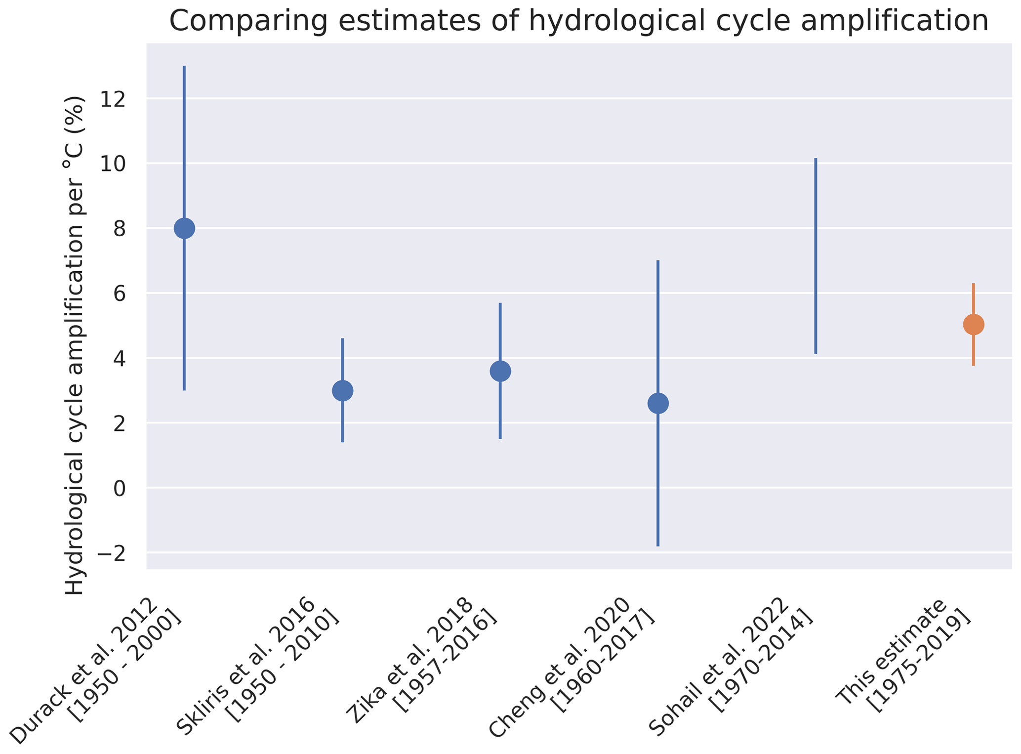
Figure 11 Comparison of this estimate of hydrological cycle amplification with previous studies. Here, we scaled the Sohail et al. (2022) estimate using the change in surface air temperature from NASA GISS data so that it could be compared against the other estimates shown (GISTEMP Team, 2023). The change in surface air temperature is found based on the linear trend over 1970–2014.

5 Conclusions

Accurate estimates of the amplification of the hydrological cycle over the historical period is important for future projections. However, freshwater flux trends cannot be measured directly and trends must be inferred, generally from ocean salinity changes. Here, we introduced a method, based on linear response theory, that infers freshwater fluxes from the evolving surface salinity pattern, building on previous studies (Durack et al., 2012; Zika et al., 2018). Our methodology flexibly accounts for regional changes in surface salinity due to different forcings (heat flux, freshwater flux, and wind stress). We therefore relax the previous assumptions from Durack et al. (2012) and Zika et al. (2018) which impose a linear scaling of the climatological salinity pattern. In particular, our method can account for the subtropical salinity changes resulting from circulation change induced by heat flux forcing (Gregory et al., 2016; Todd et al., 2020).

We validated our methodology using data from the CESM large ensemble. We recovered the true freshwater flux change (as determined from the model E−P) for CESM ensemble average data over 1975–2019. We similarly recovered the true freshwater flux change for individual ensemble members, provided that significance criteria on salinity trends were met. Thus, our method performs well on test data and can be applied to observations.

The recovery of the true freshwater flux change for individual ensemble members implies that linear response theory, under certain circumstances, can be applied to individual realizations (e.g., observations) by creating an artificial ensemble following McKinnon et al. (2017). This idea could be used for other applications of linear response theory in climate science, which has previously been limited by the need for an ensemble average, and adds to previous literature on linear response theory applied to climate (Lucarini and Sarno, 2011; Lembo et al., 2020; Ragone et al., 2016; Torres Mendonça et al., 2021).

Over the period 1975–2019, from ocean tracer observations, we estimate a change in surface freshwater fluxes equivalent to 0.3278±0.0828 times the FAFMIP perturbation. For comparison with previous studies, we convert this to 5.036±1.272 % °C⁻¹, scaling by the ECCO state estimate as the climatological hydrological cycle. After this scaling, our result is largely in agreement with previous work (Skliris et al., 2016; Zika et al., 2018; Cheng et al., 2020; Sohail et al., 2022). We also estimate a heat flux increase of 0.5938±0.1305 W m⁻² in agreement with previous studies (Gulev et al., 2021; Cheng et al., 2022). In this work, we accounted for the regional imprint of ocean circulation on salinity, yet we found a value of hydrological cycle amplification similar to that of Zika et al. (2018) which assumed that the impact of heat fluxes on the surface salinity pattern is a linear scaling of the climatological salinity pattern. This implies that over the time period considered, it may be sufficient to use this assumption of scaling the existing pattern. However, as ocean circulation changes increase due to increased anthropogenic forcing, this assumption may not hold, and our method, which accounts for regional changes, can be employed.

Our hydrological cycle amplification estimate is subject to a number of caveats indicating that the methodology may underestimate error. The error bars reported should be interpreted as a lower bound on error for the following reasons: (1) we do not quantify the uncertainty associated with utilizing different ocean models as the response functions, (2) we do not account for error in the salinity and temperature observations themselves, (3) the artificial ensemble is not equivalent to a true ensemble average, and (4) the method assumes that the change in freshwater fluxes in observations is well approximated by scaling the magnitude of the FAFMIP perturbation. Additionally, our assumption that the impact of total anthropogenic forcing can be broken into the summation of the impact of heat fluxes, freshwater fluxes, and wind stress change holds, except for the response in the saltiest region in the HadOM3 model. This exception may slightly bias results. Despite these caveats, our method performed well on CESM test data and our estimate based on observations agrees with previous studies. Thus, this work, which accounts for regional effects of ocean transport change, adds confidence to the conclusion that the hydrological cycle is amplifying at a rate less than that of Clausius–Clapeyron. This result warrants further investigation into the mechanisms controlling the hydrological cycle amplification rate and the representation in models.

Appendix A: More details on discretization and solution of the linear response problem

In the case of an ensemble average of observables, the equation that we solve at each time step to find $[\frac{\mathrm{d}{F}^{\text{h}}}{\mathrm{d}t},\frac{\mathrm{d}{F}^{\text{w}}}{\mathrm{d}t},\frac{\mathrm{d}{F}^{\text{s}}}{\mathrm{d}t}]$ is given in the main text (Eq. 6). Here, we show the explicit steps for the solution. First, we rewrite the equation as

$$\begin{array}{rl}& \langle \mathrm{\Delta }\mathit{Y}\rangle \left(t\right)-\sum _{k=\mathrm{0}}^{m-\mathrm{1}}{\mathit{R}}^{\text{h}}(m-k){\displaystyle \frac{\mathrm{d}{F}^{\text{h}}}{\mathrm{d}t}}\left(k\right)-\sum _{k=\mathrm{0}}^{m-\mathrm{1}}{\mathit{R}}^{\text{w}}(m-k){\displaystyle \frac{\mathrm{d}{F}^{\text{w}}}{\mathrm{d}t}}\left(k\right)\\ & -\sum _{k=\mathrm{0}}^{m-\mathrm{1}}{\mathit{R}}^{\text{s}}(m-k){\displaystyle \frac{\mathrm{d}{F}^{\text{s}}}{\mathrm{d}t}}\left(k\right)={\mathit{R}}^{\text{h}}\left(\mathrm{0}\right){\displaystyle \frac{\mathrm{d}{F}^{\text{h}}}{\mathrm{d}t}}\left(m\right)\\ & +{\mathit{R}}^{\text{w}}\left(\mathrm{0}\right){\displaystyle \frac{\mathrm{d}{F}^{\text{w}}}{\mathrm{d}t}}\left(m\right)+{\mathit{R}}^{\text{s}}\left(\mathrm{0}\right){\displaystyle \frac{\mathrm{d}{F}^{\text{s}}}{\mathrm{d}t}}\left(m\right),\end{array}$$

so that at time step m, the left side has only known information and unknowns are on the right side. This could be expressed as

$$\begin{array}{}\text{(A1)}& \begin{array}{rl}& \langle \mathrm{\Delta }\mathit{Y}\rangle \left(t\right)-\sum _{k=\mathrm{0}}^{m-\mathrm{1}}{\mathit{R}}^{\text{h}}(m-k){\displaystyle \frac{\mathrm{d}{F}^{\text{h}}}{\mathrm{d}t}}\left(k\right)-\sum _{k=\mathrm{0}}^{m-\mathrm{1}}{\mathit{R}}^{\text{w}}(m-k){\displaystyle \frac{\mathrm{d}{F}^{\text{w}}}{\mathrm{d}t}}\left(k\right)\\ & -\sum _{k=\mathrm{0}}^{m-\mathrm{1}}{\mathit{R}}^{\text{s}}(m-k){\displaystyle \frac{\mathrm{d}{F}^{\text{s}}}{\mathrm{d}t}}\left(k\right)=\mathbf{A}\mathit{x},\end{array}\end{array}$$

where A is a 2n×3 matrix with each column one of the R(0) vectors and x a 3×1 vector of $[\frac{\mathrm{d}{F}^{\text{h}}}{\mathrm{d}t},\frac{\mathrm{d}{F}^{\text{w}}}{\mathrm{d}t},\frac{\mathrm{d}{F}^{\text{s}}}{\mathrm{d}t}{]}^T$. This is an overdetermined system of the form b=Ax and we solve for x in the least squares sense, using the normal equations.

The method of solution is similar in the case of observations (an individual ensemble member) for which we have generated artificial ensembles. Here, for each ith artificial ensemble member, we rearrange Eq. (8) as

$$\begin{array}{rl}& \mathrm{\Delta }{\mathit{Y}}_i\left(t\right)-\sum _{k=\mathrm{0}}^{m-\mathrm{1}}{\mathit{R}}^{\text{h}}(m-k){\displaystyle \frac{\mathrm{d}{F}_i^{\text{h}}}{\mathrm{d}t}}\left(k\right)-\sum _{k=\mathrm{0}}^{m-\mathrm{1}}{\mathit{R}}^{\text{w}}(m-k){\displaystyle \frac{\mathrm{d}{F}_i^{\text{w}}}{\mathrm{d}t}}\left(k\right)\\ & -\sum _{k=\mathrm{0}}^{m-\mathrm{1}}{\mathit{R}}^{\text{s}}(m-k){\displaystyle \frac{\mathrm{d}{F}_i^{\text{s}}}{\mathrm{d}t}}\left(k\right)={\mathit{R}}^{\text{h}}\left(\mathrm{0}\right){\displaystyle \frac{\mathrm{d}{F}_i^{\text{h}}}{\mathrm{d}t}}\left(m\right)\\ & +{\mathit{R}}^{\text{w}}\left(\mathrm{0}\right){\displaystyle \frac{\mathrm{d}{F}_i^{\text{w}}}{\mathrm{d}t}}\left(m\right)+{\mathit{R}}^{\text{s}}\left(\mathrm{0}\right){\displaystyle \frac{\mathrm{d}{F}_i^{\text{s}}}{\mathrm{d}t}}\left(m\right)+\mathit{\eta }\left(t\right),\end{array}$$

so that again, at time step m, the left side contains known information and unknowns are on the right. We solve this equation in the same way as with Eq. (A1) in the least squares sense for $[\frac{\mathrm{d}{F}_i^{\text{h}}}{\mathrm{d}t},\frac{\mathrm{d}{F}_i^{\text{w}}}{\mathrm{d}t},\frac{\mathrm{d}{F}_i^{\text{s}}}{\mathrm{d}t}]$, except we neglect η(t). Then, as described in Sect. 2, we approximate the forcings $[\frac{\mathrm{d}{F}^{\text{h}}}{\mathrm{d}t},\frac{\mathrm{d}{F}^{\text{w}}}{\mathrm{d}t},\frac{\mathrm{d}{F}^{\text{s}}}{\mathrm{d}t}]$ as the ensemble average of $[\frac{\mathrm{d}{F}_i^{\text{h}}}{\mathrm{d}t},\frac{\mathrm{d}{F}_i^{\text{w}}}{\mathrm{d}t},\frac{\mathrm{d}{F}_i^{\text{s}}}{\mathrm{d}t}]$ as Eq. (9) implies.

Appendix B: Finding the change in time series

Throughout the study, we need to quantify the change in a time series while accounting for internal variability. The process is outlined as a list in Sect. 3.3, which we restate here:

1. Fit a linear trend to the relevant time series.

2. Block bootstrap around this trend with blocks of size 2 years to account for internal variability.

3. Refit linear trends to each block bootstrapped time series (totaling 3000 time series).

4. Estimate the mixture distribution for the trends of the 3000 time series.

5. Calculate the mean and standard deviation of the mixture distribution.

6. Compute the change in the time series by multiplying the mean and standard deviation of the trend by the length of the series (here, 45 years).

In step 5, we find the mean and standard deviation of the mixture distribution made up of (3000) Gaussians, where the mean and standard deviation of each Gaussian comes from the refit linear trend and associated uncertainty in that linear trend, respectively. The mean and standard deviation of a mixture distribution can be written as follows (Frühwirth-Schnatter, 2006):

$$\begin{array}{}\text{(B1)}& {\displaystyle }\mathit{\mu }& {\displaystyle }=\sum _{k=\mathrm{1}}^n{\mathit{\mu }}_k{w}_k\text{(B2)}& {\displaystyle }\mathit{\sigma }& {\displaystyle }=\sum _{k=\mathrm{1}}^n({\mathit{\mu }}_k^{\mathrm{2}}+{\mathit{\sigma }}_k^{\mathrm{2}})w_k-{\mathit{\mu }}^{\mathrm{2}},\end{array}$$

where n is the number of component distributions (here, 3000), w_k are the weights (here, $\frac{\mathrm{1}}{\mathrm{3000}}$ for each), and μ_k and σ_k are the mean and standard deviation of the k^th component distribution. We apply Eqs. (B1) and (B2) in step 5.

Note that after step 3, we could simply take the mean and standard deviation across the new linear trends without considering them as a mixture distribution. However, each refit linear trend also has some associated uncertainty. Thus, we view them as making up a mixture distribution to account for this additional uncertainty in our final standard deviation.

Appendix C: Representing freshwater flux perturbation as percentage change

The methodology described in Sects. 2 and 3 solves for the freshwater flux forcing as a proportion of the FAFMIP perturbation field. To compare with other estimates, this is converted to a percent change by comparing it against a climatological value from the ECCO state estimate. We quantify the strength of the E−P pattern by taking the area integral of the absolute value of the annual mean pattern (i.e., for the FAFMIP perturbation, the integral of the absolute value of the map in Fig. 2b). This yields a value in kg s⁻¹ that can be converted to a value in Sverdrups (Sv). We quantify the strength of the climatological pattern by taking the mean of the ECCO freshwater fluxes from 1992 to 2001 and taking the area integral in the same way. Thus, the result can be written as a percentage change by using

$$\begin{array}{}\text{(C1)}& {\displaystyle \frac{a{\int }_{\mathrm{\Omega }}\left|\mathbf{N}\right(x,y\left)\right|\mathrm{d}A}{{\int }_{\mathrm{\Omega }}\left|\mathbf{ECCO}\right(x,y\left)\right|\mathrm{d}A}},\end{array}$$

where Ω is the ocean surface south of 65° N, N(x,y) is the map of the annual mean FAFMIP freshwater fluxes perturbation, ECCO(x,y) is the map of the ECCO freshwater fluxes averaged over the period 1992–2001, and a is the proportion of the FAFMIP flux field as found by linear response theory. We can express this quantity per degree Celsius by dividing by the change in surface air temperature over the period 1975–2019 (GISTEMP Team, 2023).

Appendix D: Sensitivity to block bootstrapping choices

Here, we show results for the sensitivity of the estimate from observations (see Sect. 4) to choices in the block bootstrapping step of the methodology. As discussed in the text, we find that the result is insensitive to the block size used (Fig. D1) and to the number of artificial ensemble members created (Fig. D2).

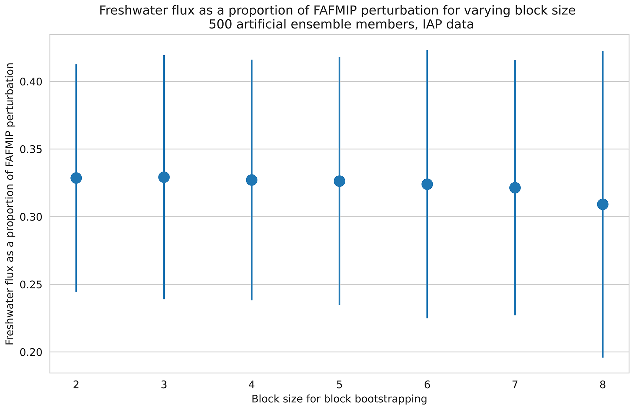
Figure D1 The freshwater flux change as a proportion of the FAFMIP perturbation (y axis) versus block size used when generating the artificial ensemble (x axis). Here, we applied the method to the IAP data over the period 1975–2019 and used artificial ensembles with 500 members.

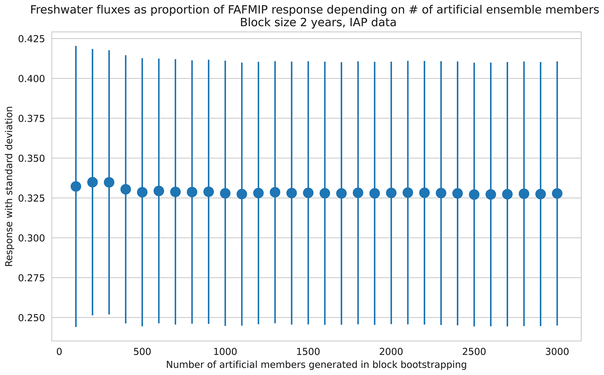
Figure D2 The freshwater flux change as a proportion of the FAFMIP perturbation (y axis) versus number of artificial ensemble members (x axis). Here, we applied the method to the IAP data over the period 1975–2019 and used a block size of 2 years.