the Creative Commons Attribution 4.0 License.
the Creative Commons Attribution 4.0 License.
 | 27 Mar 2024
Solar radiation modification challenges decarbonization with renewable solar energy
Benjamin M. Sanderson
Roland Séférian
Laurent Terray
Solar radiation modification (SRM) is increasingly being discussed as a potential tool to reduce global and regional temperatures to buy time for conventional carbon mitigation measures to take effect. However, most simulations to date assume SRM to be an additive component to the climate change toolbox, without any physical coupling between mitigation and SRM. In this study we analyze one aspect of this coupling: how renewable energy (RE) capacity, and therefore decarbonization rates, may be affected under SRM deployment by modification of photovoltaic (PV) and concentrated solar power (CSP) production potential. Simulated 1 h output from the Earth system model CNRM-ESM2-1 for scenario-based experiments is used for the assessment. The SRM scenario uses stratospheric aerosol injections (SAIs) to approximately lower global mean temperature from the high-emission scenario SSP585 baseline to the moderate-emission scenario SSP245. We find that by the end of the century, most regions experience an increased number of low PV and CSP energy weeks per year under SAI compared to SSP245. Compared to SSP585, while the increase in low energy weeks under SAI is still dominant on a global scale, certain areas may benefit from SAI and see fewer low PV or CSP energy weeks. A substantial part of the decrease in potential with SAI compared to the SSP scenarios is compensated for by optically thinner upper-tropospheric clouds under SAI, which allow more radiation to penetrate towards the surface. The largest relative reductions in PV potential are seen in the Northern and Southern Hemisphere midlatitudes. Our study suggests that using SAI to reduce high-end global warming to moderate global warming could pose increased challenges for meeting energy demand with solar renewable resources.
- Article
(5040 KB) - Full-text XML
-
Supplement
(5592 KB) - BibTeX
- EndNote


With a rapidly dwindling remaining carbon budget for the Paris 1.5 °C temperature goal, a growing set of literature has been investigating the potential of temporarily reducing climate change impacts with solar radiation modification (SRM), also known as solar geoengineering (UNEP, 2023). SRM is a term describing a set of technologies which temporarily cool the climate by modifying the balance of incoming versus outgoing radiation (Boucher et al., 2013; Budyko, 1977; Crutzen, 2006; Irvine et al., 2016). Proposed methods include changing properties of high-lying (Mitchell and Finnegan, 2009) or low-lying (Latham, 1990) clouds, injecting reflective aerosols into the stratosphere (Boucher et al., 2013), and placing objects in space that deflect some of the sun's radiation that reaches the Earth's surface (Angel, 2006). The idea behind SRM is to use one or a combination of these technologies until emissions have been sufficiently reduced and carbon removal technologies scaled up to keep temperatures at an acceptable level without SRM. This “buying time” approach hinges critically on the premise of decarbonization during SRM in which a carbon-free energy supply from renewable sources plays an essential role. However, while there is a growing number of studies on the socioeconomic effect of SRM on mitigation (Belaia et al., 2021; Bellamy et al., 2016; Burns et al., 2016; Keith, 2000; McLaren, 2016; Merk et al., 2016; Moreno-Cruz, 2015; Wibeck et al., 2015), the so-called moral hazard risk, so far, few studies have assessed whether SRM affects our decarbonization potential in physical terms. Here, we target the question of changes in renewable energy (RE) generation potential in the case of solar-based RE technologies, as well as photovoltaic (PV) and concentrated solar power (CSP), under SRM.
A change in solar RE productivity is especially interesting since most SRM methods act on reducing incoming energy, while PV and CSP use incoming energy to turn into electricity. The reduction in solar radiation through SRM is therefore believed to have negative effects for solar RE power production (Robock, 2008; Robock et al., 2009). A pronounced effect is expected for CSP under stratospheric aerosol injection interventions, since CSP relies on direct shortwave radiation for its energy production, but the addition of aerosols shifts the ratio of direct and diffuse radiation to entail a larger diffuse fraction. PV panels, on the other hand, can convert both direct and diffuse shortwave radiation into electrical energy with similar efficiency depending on the specific PV technology used (Parretta et al., 2003) and the tilt of the installation (Khan et al., 2022). However, while solar RE electricity generation depends substantially on solar irradiance, other atmospheric variables such as temperature and wind influence PV panel and CSP efficiency.
Most studies to date have estimated the global and regional potential of solar RE and change thereof as a result of global warming. Climate change influences solar energy resources through changes in atmospheric water vapor content, cloudiness and cloud characteristics (Schaeffer et al., 2012; Clarke et al., 2022; Scheele and Fiedler, 2023), and aerosols (Clarke et al., 2022; Scheele and Fiedler, 2023), i.e., atmospheric transmissivity. At a global scale, solar resources are projected to decrease slightly compared to current values (Huber et al., 2016; Crook et al., 2011; Wild et al., 2015), and, in general, power output from CSP plants seems to be more sensitive to climate change than PV plants (Huber et al., 2016). However, electricity production from PV and CSP is not just driven by solar resources, but also by other factors such as surface air temperature and aerosols (Schaeffer et al., 2012; Clarke et al., 2022; Scheele and Fiedler, 2023). Regional differences in the development of these variables cause variations in electricity output trends around the world (Scheele and Fiedler, 2023). Increases in PV and CSP output are projected across Europe, the eastern US and East Asia (Crook et al., 2011; Gernaat et al., 2021; Tobin et al., 2018; Wild et al., 2015; Zou et al., 2019), whereas Africa, Saudi Arabia, Australia, and central and Southeast Asia show decreases (Crook et al., 2011; Gernaat et al., 2021; Wild et al., 2015). However, not all studies agree on the sign of changes and regional analyses in particular show much greater variability (Bartók et al., 2017; Bazyomo et al., 2016; Huber et al., 2016; Jerez et al., 2015; Tobin et al., 2018).
So far, to our knowledge, only two studies have been conducted on solar RE and SRM. Murphy (2009) investigated the effect of stratospheric aerosols on CSP production, concluding that an enhancement of the aerosol layer would lead to a reduction in the efficiency of CSP systems by 4 % to 10 % for each 1 % reduction in total sunlight reaching the Earth (Murphy, 2009). More recently, Smith et al. (2017) studied PV and CSP potential under stratospheric sulfate injections and found an overall reduction in CSP output of 4.7 % to 5.9 % on land relative to a scenario without geoengineering and a reduction in PV potential of 1 % to 3 % over land depending on the model and type of PV technology (Smith et al., 2017).
In this study we calculate and compare PV and CSP potential under a geoengineered world versus one that is moderately ambitiously mitigated to approximately the same global mean temperature (SSP245) and also versus an unmitigated, fossil-fuel-intensive climate change scenario (SSP585). The method of SRM considered in this study is stratospheric aerosol injection (SAI).
2.1 PV and CSP potential
In this paper we use the term potential to refer to an enhanced version of the standard definition of the technical potential. The technical potential is defined as the theoretical potential, which is the upper limit based on geophysical conditions, i.e., the total energy from solar irradiance on Earth, constrained by geographical and technical restrictions. Geographical constraints restrict the theoretical potential to areas that are considered to be physically and regulatorily suitable for PV or CSP production, while technical restrictions refer to efficiency losses during the transformation of primary energy flux to secondary resource (de Vries et al., 2007). Here, we add an additional geographical constraint to the technical potential by weighting the area cells according to the proximity to highly populated cells (see Sect. 2.2 on geographical restrictions).
2.1.1 Data and simulations
We calculate the potential for three different scenarios: SSP245, a scenario representing approximate current policy (O'Neill et al., 2016); SSP585, a very high-emission scenario (O'Neill et al., 2016); and G6sulfur, an SRM scenario that imitates stratospheric aerosol injections (SAI) (Kravitz et al., 2015) and will be referred to as SAI in this study. G6sulfur has the starting conditions and underlying emissions of SSP585 but uses SAI to match the global radiative balance of SSP245 until 2100. G6sulfur is part of the GeoMIP protocol (Kravitz et al., 2015), but here, the setup is enhanced with higher-frequency output and additional variables related to radiation and wind. We run the scenarios using the Earth system model CNRM-ESM2-1 with prescribed aerosol optical depth derived from the GeoMIP experiment G4SSA (Tilmes et al., 2015) to simulate the aerosol injections in G6sulfur/SAI. Three-member ensembles of G6sulfur/SAI, SSP245 and SSP585 from CNRM-ESM2-1 exist already but are not used here. Instead, for this study, we repeated the simulations with an alternative version of CNRM-ESM2-1 (Séférian et al., 2019) that accounts for the aerosol–light interaction. This additional feature of the model enables a change in the partition of direct and diffuse light due to a change in aerosol concentration in the whole atmospheric column. We run a six-member ensemble with initial condition perturbations as for the standard SSP simulations for all three scenarios in concentration-driven mode. The simulations cover the 2015–2100 period and output data are saved at an hourly frequency. The global mean aerosol optical depth required in the SAI simulation to get from SSP585 to SSP245 reaches 0.35 in the last decade. We bilinearly regrid the model output to match the resolution of the land use data described in Sect. 2.2. Region allocation for the regional analysis follows the IPCC sixth assessment report working group I reference set (Iturbide et al., 2020), which distinguishes between 46 land regions. In this study, we exclude East and West Antarctica. The calculation of the cloudy-sky radiation involves the subtraction of clear-sky downwelling shortwave radiation from the total downwelling shortwave radiation. The clear-sky downwelling shortwave radiation is a variable that excludes the effect of clouds, but includes aerosols, and is saved by the model. To account for the solar geometry for the fixed-tilt PV panel configuration, the 1h solar zenith θz and solar azimuth α angles were calculated offline.
2.1.2 Photovoltaic potential on horizontal plane
The technical potential for PV (PVTP) for grid cell i (kWh yr−1) is calculated in line with previous studies (e.g., Dutta et al., 2022; Gernaat et al., 2021; Köberle et al., 2015; Scheele and Fiedler, 2023) as follows:
with RSDSi being the shortwave downwelling radiation at the Earth's surface, h the hours in a year, Ai the suitability factor for the grid cell, ai the area of the grid cell, nLPV the land use factor, meaning the area covered by panels, nPV,i the PV panel efficiency, and PR the performance ratio that expresses the difference between performance under standard test conditions (STCs) and the actual output of the system due to losses from suboptimal angles, dust and dirt or cable and inverter losses (85 %) (Fraunhofer ISE, 2023). The conditions under the STC are a cell temperature of 25 °C, solar irradiance of 1000 Wm−2 and an air mass spectrum of 1.5 (AM1.5). A collection of all variables and their descriptions, units and sources is provided in Table S1. Equation (2) accounts for changes in efficiency through climate variables:
We have selected the widely used monocrystalline silicon PV panel as our reference panel (Dutta et al., 2022; Jerez et al., 2015; Sawadogo et al., 2021; Feron et al., 2021) whose 2023 panel efficiency under STC is at 26.8 % (nPanel) (Fraunhofer ISE, 2023; NREL, 2023) but may be modified under different temperature conditions (Radziemska, 2003), resulting in nPV,i. γ represents the efficiency response of monocrystalline silicone PV panels, TSTC is the temperature of the panel under STC, i.e., 25 °C, and Tp,i is the actual temperature of the panel, calculated as
with c1, c2, c3 and c4 as constants that are described in Table S1. Ti is the surface air temperature, RSDSi downwelling shortwave radiation and Vi surface wind velocity. The PV cell temperature Tp,i can be significantly higher than the ambient air temperature Ti under sunny conditions. Total power output is reduced by 0.37 % per 1 °C increase in cell temperature for monocrystalline cells depending on its temperature coefficient (Mahdavi et al., 2022; Rahman et al., 2015).
2.1.3 Photovoltaic potential with fixed-tilt panels
To account for the angle with which the shortwave radiation strikes tilted panels, we conduct an additional PV potential calculation that considers the solar geometry and the partitioning of direct and diffuse radiation, instead of using total horizontal downwelling radiation as in Sect. 2.1.2. We follow the approach in Smith et al. (2017) and calculate direct radiation as
with RSDSdir as direct downwelling shortwave radiation, RSDSdiff diffuse downwelling shortwave radiation and θz the 1 h mean solar zenith angle.
We consider the inclination of the panels to be equal to latitude oriented towards the Equator and calculate the radiation on the tilted panel RSDSpanel,i in line with Smith et al. (2017):
Here, θpanel is the angle with which the direct radiation strikes the tilted panel and β the tilt of the panel, i.e., the latitude. cos θpanel depends on the latitude, solar zenith and solar azimuth angle and is taken as
We calculate PVTP,fixed using Eqs. (1), (2) and (3) but replacing RSDS with RSDSpanel in Eqs. (1) and (3). The calculation with fixed-tilt panels is used in Fig. 4. All other analyses are based on horizontally aligned panels.
2.1.4 Concentrated solar power potential
The technical potential for CSP (CSPTP) is (Gernaat et al., 2021; Köberle et al., 2015)
RSDSdir,i is downwelling direct shortwave radiation and nLCSP the land use factor. The full load hours FLHi are calculated according to Köberle et al. (2015) as
and the CSP efficiency corrected for atmospheric variables, nCSP,i, as (Gernaat et al., 2021; Dutta et al., 2022)
with nR as the efficiency of the Rankine cycle (40 %), Tf the temperature of the heat transfer fluid (115 °C), and k0 and k1 as constants described in Table S1.
Only areas with a 10-year average daily RSDSdir of minimum 4 kWh m−2 are taken into account, similar to Köberle et al. (2015), Trieb et al. (2009) and Hernandez et al. (2015).
2.2 Geographical restrictions
The installation of PV and CSP is subject to geographical constraints such as regulatory constraints, the prevalent land use and distance to demand, the restriction to onshore areas, and, for CSP, the solar resources described in Sect. 2.1.3. Figure 1 shows the convolution of the area weights used in the calculation of the renewable energy potential (see variable Ai in Sect. 2.1); the single area restrictions and their weights are displayed in Fig. S1. We remove all areas marked as protected with any status as characterized by the United Nations Environment Programme (IUCN, 2023) as possible solar power installation sites and weigh areas according to the prevalent land use and distance to highly populated centers as an indicator for the future existence of transmission lines and demand.
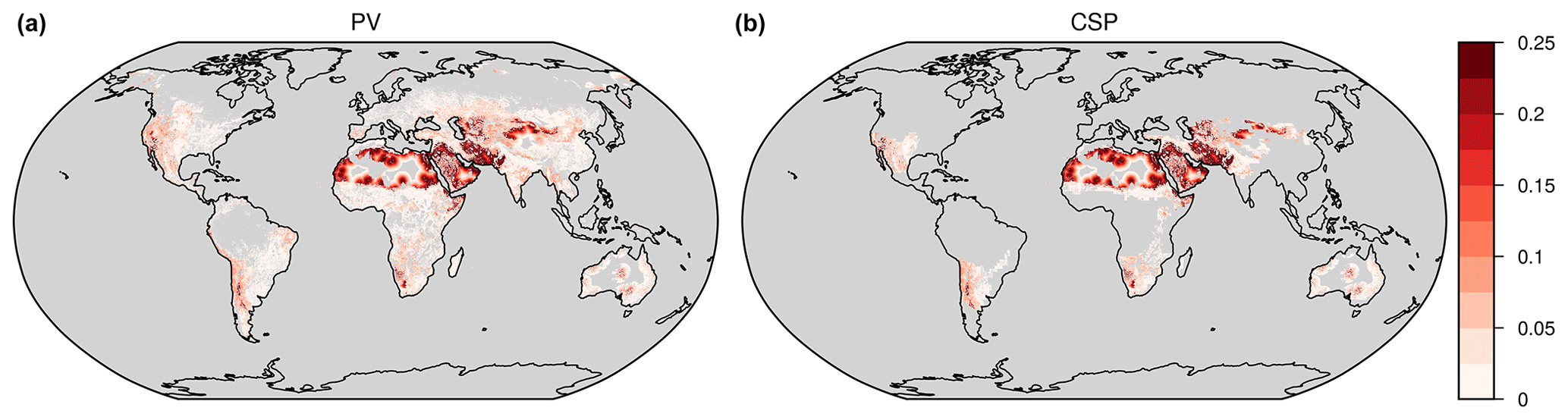
Figure 1Area weights applied to (a) PV and (b) CSP. Weights shown are calculated using SSP2 assumptions.
Land use and population density data are taken from the IMAGE3.0-LPJ model (Doelman et al., 2018; Stehfest et al., 2014). IMAGE3.0-LPJ has a spatial resolution of 0.1° × 0.1° and distinguishes between 20 different land use and land cover types. We weight each land use and land cover category by the fraction of each grid cell that could be covered by solar renewable energy technology (Ai), similarly to Hoogwijk (2004), but with different land use categories and different fractions assigned (see Table S2 for land use categories and assigned suitability fractions). The underlying idea is that only part of a grid cell is available for solar RE installations as it may compete with other land uses such as agricultural production or ecosystem services from forests. Another influencing factor is the perceived difficulty of preparing the land for such installations. A suitability fraction of 10 % means 10 % of the grid cell could be covered with a CSP plant or PV farm. It does not, however, imply that 10 % of the area is covered by panels, meaning that 10 % of the radiative energy can be harvested.
We weight the distance to densely populated areas from the IMAGE3.0-LPJ model (Doelman et al., 2018; Stehfest et al., 2014) using a sigmoidal function. The data come in 5-year steps and are aggregated to 10-year means for our calculations. The weight decreases as the distance to the densely populated grid cells increases until it reaches a weight of 0 at a distance of about 500 km, an arbitrarily chosen cut-off.
The maps and numbers shown in the main paper are calculated using equal weights across all scenarios and years. Please consult the Supplement for figures where area weighting (land use suitability and population assumption) is chosen according to scenario (SSP2 for SSP245; SSP5 for SSP585 and SAI). Figure S2 shows the difference in land use suitability fractions, population density weighting and total area weighting between the scenarios. Figure S3 displays the difference in the same variables for the present (2015–2024) versus the future (2090–2099).
2.3 Low energy week (LEW)
The low energy week (LEW) metric assesses whether an area shows a change in weekly energy output that is particularly low. This is of interest for energy production as prolonged periods of extremely low production may have greater significance than a slight reduction from high-production days to medium production. The LEW metric calculates the number of weeks per year in 2095–2099, where the weekly sum is below the 20th percentile of current (2015–2019) seasonal average weekly sums,
and s indicates the season, y the number of years, h the number of hours per week, P20 the 20th percentile, M the number of ensemble members and the mean over x. The boundaries of the 7 d period are fixed. Please note that in figures related to LEWs the color bars are reversed compared to the figures related to long-term mean changes. This choice was made because in this case negative values imply a positive outcome for energy production.
3.1 Change in 2090–2099 average PV and CSP potential
On a global scale, the sign of the change in PV potential under SAI compared to SSP245 or SSP585 is negative (Fig. 2a–c). Globally, PV potential is on average 4.1 % lower under SAI than SSP245 and 1.4 % lower under SAI than SSP585. Regionally, this decrease varies from −8 % to 0 % for SSP245 to SAI and −6 % to +4 % in the case of SSP585 to SAI. The largest absolute losses for SAI are in the northern midlatitudes for SSP585 (−2.5 PWh yr−1) and the tropical region of the Northern Hemisphere for SSP245 (−19.0 PWh yr−1; Fig. 2c). This is likely owing to the large land mass in this latitudinal zone, much of it desert, which is very rich in solar resources. Even small relative losses in this area would be large in absolute terms.
When the area weighting is chosen according to the scenario, the changes between SSP585 and SAI remain the same because assumptions are the same, but for SSP245 there are large differences, mainly related to dissimilar population assumptions (Fig. S4).
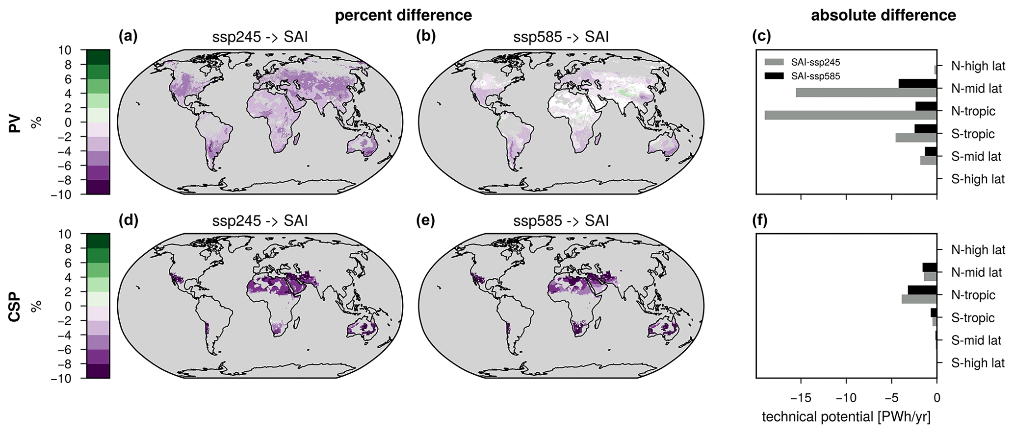
Figure 2Difference in 2090–2099 PV (a–c) and CSP (d–f) potential between the ensemble means of SAI and (a, d) SSP245, (b, e) SSP585 and (c, f) absolute difference between latitudinal zonal sums between SAI and SSP245 and SSP585 in PWh yr−1. White areas have an SNR of < 1. x−>y denotes .
The reductions in CSP are greater than those of PV for either scenario comparison. Relative to SSP245, all regions see a decline in CSP potential of 4 %–16 % under SAI. The comparison with SSP585 shows steeper declines in some areas, such as Australia, where CSP potential is up to 16 % lower under SAI than SSP585. But there are other areas where the decline is smaller than for SSP245, such as in the Middle East. Absolute losses are highest in the northern hemispheric tropics, mostly due to the large area considered suitable in this latitudinal zone. Globally, CSP potential is reduced by 7.6 % when comparing SAI and SSP245 and 7.8 % for SAI and SSP585.
Table 1 displays the total global PV potential for each scenario when considering different geographical restrictions (see Table S3 for CSP). Naturally, the potential decreases with increasing geographical restrictions. Irrespective of the constraint applied, SAI has the lowest global potential, followed by SSP585. Unsurprisingly, the potential is significantly reduced by the weighting of land use suitability. Additionally, the weighting of population density has a notable impact due to the fact that areas with the highest potential, such as deserts, are typically further away from population centers than areas with lower potential such as crops. For CSP, there is only a minimal difference between SSP245 and SSP585, but there is a considerable reduction for SAI. Without land use suitability or population density weighting SSP585 has the highest potential of the three scenarios (Table S3).
Table 1Total global 2090–2099 PV potential per scenario in PWh yr−1 under different geographical constraints.
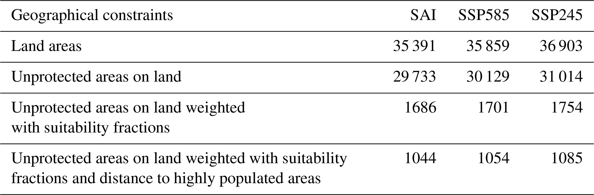
Figure 3 explains which physical variables drive the change in PV potential and create the regional variation visible in Fig. 2. When holding radiation fixed and letting temperature be the only variable that fluctuates, the difference in PV potential is very small, especially for SSP245 and SAI, where global mean temperature is at a close match (Fig. 3a–c). The regional variation change is a result of differences in surface radiation (Fig. 3d–f), with changes in cloudiness being the primary driver of variance (Fig. 3g–l). With few exceptions, the cloudy sky in SAI is much more transmissive for shortwave radiation, increasing the potential by up to 16 % for cloudy sky. Compared to SSP585, cloud cover is enhanced under SAI in some areas such as over large parts of Australia, southeastern Africa, northern Argentina, and southern United States and Mexico. However, despite SAI having fewer reflective clouds than SSP245 and SSP585, the reduction in clear-sky radiation is more pronounced. With regard to radiation, the potentials are significantly more negative when comparing to SAI than when the two SSP scenarios are compared to each other (Fig. 3g–i). This is because the principle of SAI is the reduction of incoming solar radiation. See Fig. S5 for the physical drivers of CSP.
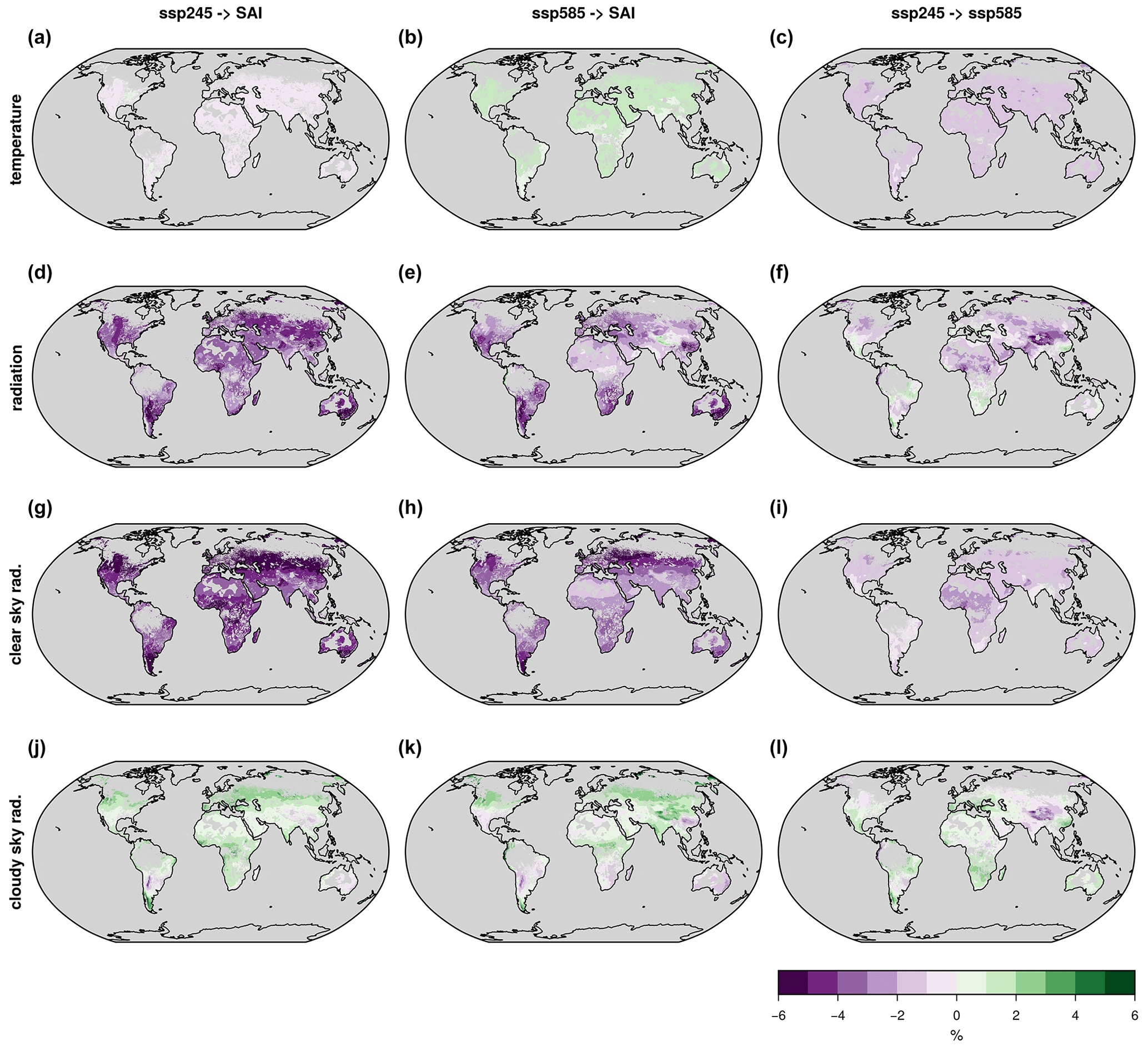
Figure 3Main drivers of change in 2090–2099 PV potential, (a–c) surface air temperature, (d–f) total downwelling surface radiation, (g–i) clear-sky radiation and (j–l) cloudy-sky radiation. Areas with SNR <1 are shown in white. x−>y denotes . (a)–(c) Calculated by keeping all variables except temperature fixed, (d)–(f) by keeping all variables except radiation fixed, (g)–(i) by using the model output clear-sky radiation instead of total radiation (see the Methods section) and (j)–(l) by subtracting clear-sky radiation from total radiation.
3.2 Change in 2090–2099 average PV potential with fixed tilted panels
Figure 4 displays the same elements as Fig. 2 but under consideration of the sun's position relative to the tilted panels. Compared to the calculation with horizontal panels, on average, more direct radiation and less diffuse radiation reach the panels (Fig. S6). This leads to more total radiative energy reaching the panels in many latitudes but particularly in the midlatitudes and especially for the SSP scenarios. Because this effect is more pronounced under the SSP scenarios than SAI, it further increases the relative and absolute difference between SAI and SSP in these higher latitudes compared to the calculation with horizontal panels (Figs. 2, 4), shifting the biggest absolute losses for SAI compared to SSP245 to the northern midlatitudes instead of the tropics. With fixed-tilt panels, total global PV potential is 6.9 % lower under SAI compared to SSP245 and 4.2 % lower compared to SSP585. Reductions under SAI are most pronounced over Russia and central Asia, the Great Plains in North America, Argentina in South America, New Zealand, and southeastern Australia.
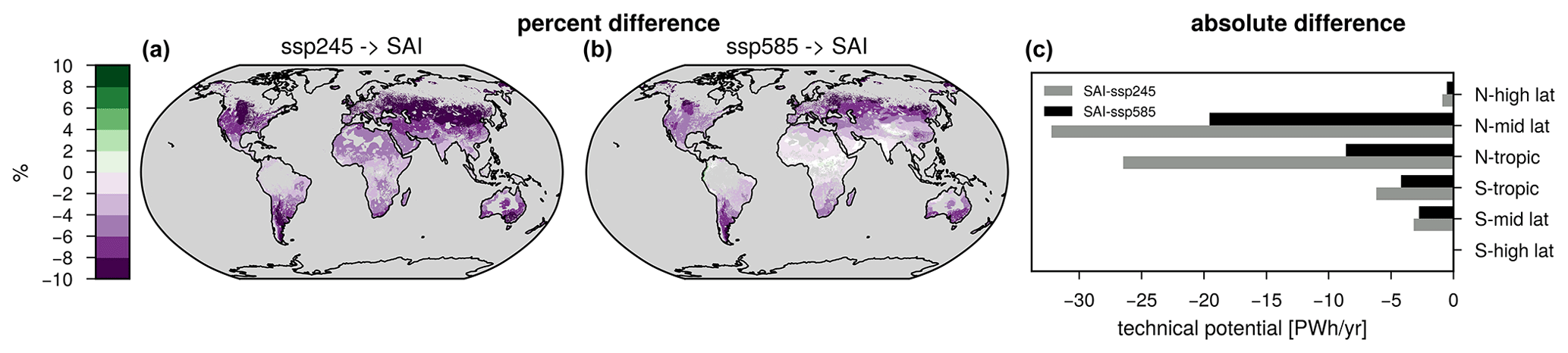
Figure 4Difference in 2090–2099 PV potential with fixed tilted panels between the ensemble means of SAI and (a) SSP245, (b) SSP585 and (c) absolute difference between latitudinal zonal sums between SAI and SSP245 and SSP585 in PWh yr−1. White areas have an SNR of <1. x−>y denotes .
3.3 Changes in potential on a regional scale and with higher frequency
The following analysis looks at changes in PV potential on more refined spatial and temporal scales. Figure 5a presents relative regional changes compared to the SSP scenarios split up into two different seasons: December, January and February (DJF) as well as June, July and August (JJA). The smallest variation in seasonal potential is in the Sahara, and the largest is in central North America for SSP245 and southern Australia for SSP585. Most regions see the largest decrease in potential in their respective hemispheric winter. Figures S7 and S8 display all 44 regions (Figs. S7, S8). When including the area weighting of the respective scenarios, some regions experience a substantial shift and in the case of northwestern North America, western North America, the Caribbean, South Asia and southern Australia even a change in the sign of difference (Fig. S9 for land use suitability difference only; Fig. S10 for land use suitability and population density difference).
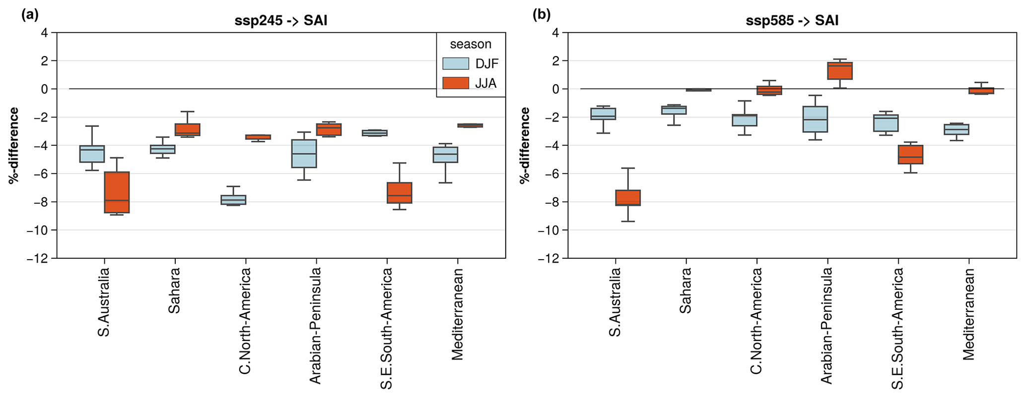
Figure 5Relative change in 2090–2099 PV potential from (a) SSP245 to SAI and (b) SSP585 to SAI for six IPCC AR6 regions (Iturbide et al., 2020) split up into two seasons: December, January, February (light blue); June, July, August (orange–red). Box plot bars represent the spread over the six ensemble members. X−>y denotes .
Further refining the temporal resolution, the maps in Fig. 6a–c show the change in PV low energy weeks (LEWs; see definition in Sect. 2.3) from the present (2015–2019) to future (2095–2099) for the three scenarios SAI, SSP245 and SSP585 when the area weighting is kept constant between the present and the future as well as between the scenarios. Please note that the color bar is reversed in this figure compared to Figs. 2, 3 and 4. We made this choice because in this case negative values imply a positive outcome for energy production. There appear to be similar regional trends among the scenarios, but the extent of change varies considerably: under each of the three scenarios, most regions see an increase in LEWs from present to future. Similarly, in all three scenarios, western China, the southern Sahara and central North America, areas with high absolute potential, see the largest increases in low-solar-resource periods, with SSP585 experiencing the largest one. Areas that are white, i.e., have up to 10 LEW yr−1, either experience a decrease in LEW compared to the present or remain constant at the present-day value.
SAI has substantially more LEWs than SSP245. Highly productive regions, such as the Saharan and East African region, Tibet and western China, Australia, Madagascar, northwestern Argentina, and the Middle East including the Arabian Peninsula, are especially affected with up to 12 additional low-resource weeks per year (Fig. 6d). The only areas with a small decline in LEWs compared to SSP245 are the south of India, the west of Spain, Portugal, and along the Argentinian and Chilean border. Compared to SSP585, SAI clearly benefits several regions by having up to eight fewer LEWs per year on the Tibetan Plateau and up to 4 weeks less in western China, the Arabian Peninsula, northern North America, and parts of the Sahara, central Africa and Russia (Fig. 6d, e). However, it exacerbates the negative trend in others, adding up to eight additional LEWs per year (eastern China, southern Africa and Madagascar, southern and central South America, Australia, and the Middle East excluding the Arabian Peninsula) (Fig. 6e). Generally, in areas that experience the most pronounced rise in LEWs from the present to future under SSP585, SAI offsets some of these increases.
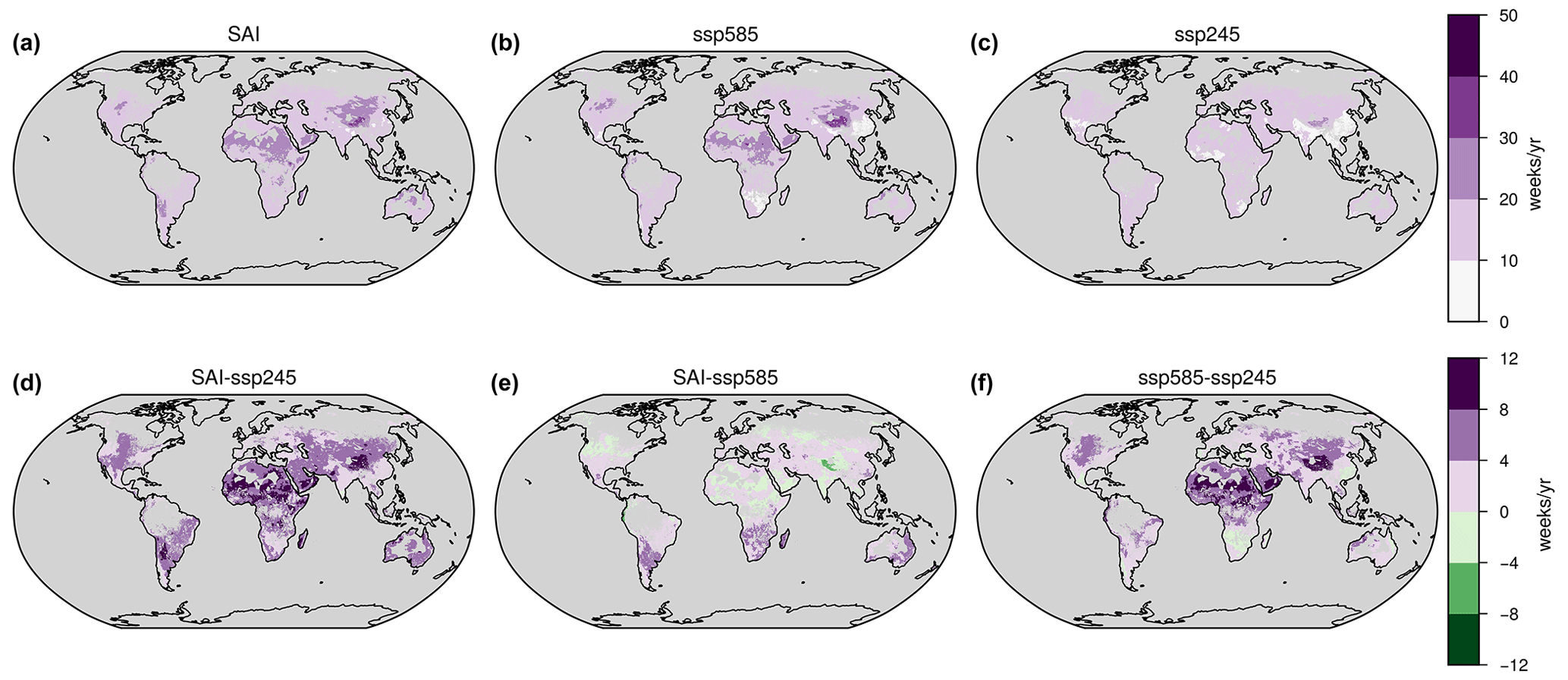
Figure 6PV low energy week metric for (a) SAI, (b) SSP585 and (c) SSP245. The LEW is calculated between the present (2015–2019) and the future (2095–2099) with equal area weighting. See Sect. 2.3 for the LEW equation. Panels (d)–(f) show the differences between (a)–(c). Color bars are reversed compared to Figs. 2, 3 and 4.
For CSP, even though relative changes are much stronger than for PV, the difference in the number of LEWs is comparable to if not less than for PV. Relative to SSP245, the Sahara, the Middle East and Australia register the largest increase in LEWs per year under SAI. Botswana and northern Namibia see a small decrease. The pattern is similar when comparing to SSP585, although here not southern Africa but the Arabian Peninsula is the most advantageous under SAI and shows a decrease in LEWs. The maps in Fig. S11d and e are confined to areas deemed suitable under SAI and exclude regions that may be considered under the SSPs but not under SAI. The signal in the maps in Fig. S11a, d and e is dominated by the fact that different areas are considered suitable for CSP in the present versus the end of the century.
Over the American continent, trends in 10-year means calculated from hourly data are consistent with weekly sums (Fig. 6d–f; see Fig. S12 present-future comparison). However, elsewhere there are clear differences: for example, one of the areas most heavily affected in relative terms of 10-year average differences from SSP245 to SAI is the south of Australia. But, in terms of LEW difference between these two scenarios, while SAI clearly records more LEWs in that region than SSP245, it is by no means the area of the highest LEW increases.
The shift from the present (2015–2024) to future (2090–2099) implies the largest drops in PV potential for SAI (4 %–8 %), with SSP585 following closely behind, whereas SSP245 displays only decreases of 0 %–4 % with certain regions experiencing an elevated potential (Fig. S12). Figure 7 illustrates the temporal evolution of the relative difference between the three scenarios and present-day values with the increase in SAI deployment intensity over time. In the first 4 decades, the scenarios differ only slightly, but the gap in potential starts to widen as time goes on. The quasi-linear increase in the gap between SAI and the SSP scenarios in some regions indicates that, in these areas, the reduction in PV potential strengthens with increasing global mean aerosol optical depth. See Fig. S13 for the temporal evolution of all 44 regions. The temporal evolutions are a lot less well-behaved with relative increases and decreases compared to the present that can be several times larger when the land use suitability area weighting is included respective to its scenarios (Fig. S14) than when it is not (Fig. S13).
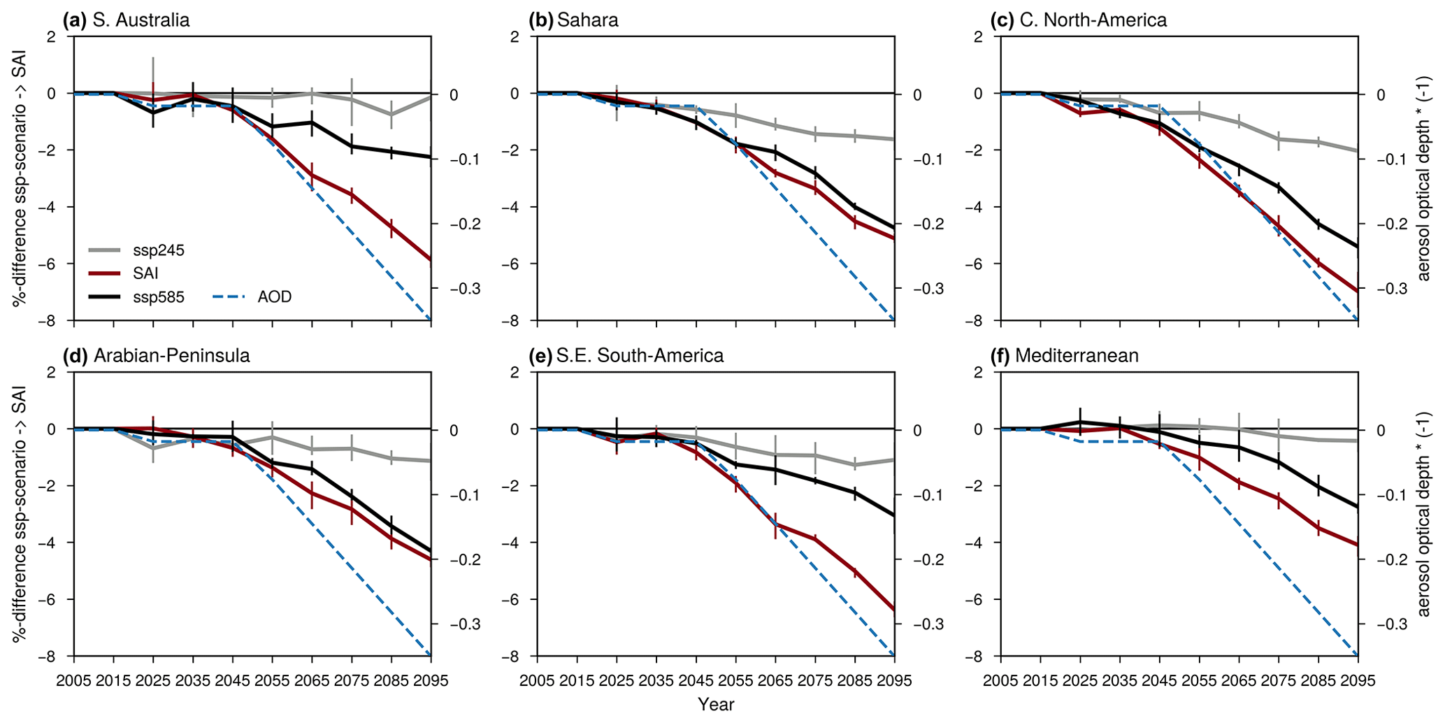
Figure 7Relative difference over time of SAI (red), SSP245 (gray) and SSP585 (black) PV potential compared to 2015–2024 values for selected regions. Lines are the ensemble means with the bars indicating the 20th–80th percentile ranges of the single members. x−>y denotes .
Current SRM scenarios rely on the assumption that, in physical terms, the decarbonization potential remains unchanged whether SRM is added to the toolbox or not. Here, we scrutinized this hypothesis by looking at changes in the potential of solar RE technology such as photovoltaic (PV) and concentrated solar power (CSP). The data suggest that when comparing an SRM world to a world where mitigation was chosen over SRM, i.e., SSP245 in our setup, almost all regions would have several additional weeks per year with low energy potential under SRM (Fig. 6). With respect to the baseline scenario SSP585, regions that are especially affected by climate change appear to benefit from SAI and exhibit fewer LEWs, but the overall trend is nevertheless an increase in LEW. When tilted panels are considered, relative and absolute losses under SAI compared to the SSP scenarios are much greater, especially in middle and high latitudes (Figs. 2, 4).
In terms of long-term changes the potential is ubiquitously reduced by several percentage points under SAI, especially for CSP (SSP245: −7.6 %) but also for PV (SSP245: −4.1 %; fixed-tilt panels SSP245: −6.9 %) (Figs. 2 a, d, 4). When comparing the SAI simulation with SSP585, the reduction in PV potential is still dominant (SSP585: −1.4 %; fixed-tilt panels SSP585: −4.2 %) but less pronounced with few regions showing insignificant differences (Figs. 2 b, 4). In contrast, the change in CSP potential between SAI and SSP585 does not differ that much from the change between SAI and SSP245 (SSP585: −7.8 %; SSP245: −7.6 %) (Fig. 2 d, e). Smith et al. (2017), the only previous study that used a modeling framework to analyze PV and CSP under geoengineering, found an average decrease in PV power output on land for fixed panels of 1 to 1.7 % and a decrease of 4.7 % to 5.9 % for CSP, depending on the climate model and without confinement to suitable locations. The greater relative losses we record are likely due to the larger temperature gap we offset with SRM in our experiments. Their study used stratospheric aerosol injections to cool global mean temperature by 1 °C from an RCP4.5 starting point, which resembles our SSP245 end point. This means that not only do we have a stronger climate change signal underlying our data, but we also use SRM to cool down more than double the temperature difference that their experiments offset, and, as Fig. 7 demonstrates for the case of PV, many regions see a quasi-linear decrease in potential the more SRM is scaled up. Other sources of discrepancy between results might lie in the different implementation of SRM in the climate models, the higher temporal resolution of our output data and the different approach in calculating PV potential. Nevertheless, in line with Smith et al. (2017) we find that the change in solar radiation due to geoengineering has a more profound effect on PV and CSP potential than changes in surface air temperature (Figs. 3, S5), and one of the two models they use, GEOSCCM, shows a similar pattern in relative PV potential changes under SAI compared to a control simulation as our results (Fig. 4).
While a decrease in PV and CSP potential was to be expected as the very nature of SRM is to reduce incoming solar radiation, there are two drivers that exert a positive impact of SAI on PV panels compared to the SSP scenarios for horizontal panel alignment. The first driver is the temperature benefit that photovoltaic panels get from colder ambient air temperatures (Dubey et al., 2013), which we observe for the difference between SAI and SSP585 (Fig. 3b). Surface air temperatures are similar between SSP245 and SAI. Thus, in this scenario, the advantages of geoengineering for photovoltaic panels in terms of temperature are practically non-existent (Fig. 3a). The second driver is the reduction in reflective cloud cover under SAI. With respect to SSP245 (Fig. 3j), this change compensates for a significant part of the decrease in PV potential. For SSP585, while overall reflective cloud cover is also lower under SAI, the difference is less pronounced and the sign of change in cloud cover is region-dependent. Here, areas with substantial reductions in PV potential correlate well with regions where cloud optical depth is actually enhanced under SAI (Fig. 3e, k). We are not the first to have observed a change in cloud cover under geoengineering: Kuebbeler et al. (2012), Cziczo et al. (2019) and Visioni et al. (2018) showed that the injection of aerosols into the stratosphere can affect upper-tropospheric clouds, making them optically thinner (Kuebbeler et al., 2012; Cziczo et al., 2019; Visioni et al., 2018). The main drivers of this effect are the reduced vertical temperature gradient in the troposphere, which leads to a decreased ice supersaturation probability and thereby a decreased ice particle number density and optical thickness (Kuebbeler et al., 2012; Visioni et al., 2018), and the aerosols themselves (e.g., Visioni et al., 2021). These optically thinner upper-tropospheric clouds allow more shortwave radiation to propagate downwards, which leads to the radiation compensating effect seen in Fig. 3j and k. Visioni et al. (2021) illustrate the global pattern of total cloud cover differences between an SAI simulation that compensates for the temperature increase above present values under RCP8.5 conditions and the control run close to the present period. The simulations were performed with CESM-WACCM. Not only did they find a dominant reduction in total cloud cover under the aerosol injections, but, similar to our results, their experiments show increased cloudiness in areas such as Australia, northwestern South America and parts of China. This pattern, although not perfectly identical, correlates well with the cloud effects observed in our results (Fig. 3j, k). The decreased potential under SSP585 compared to SSP245 for clear-sky calculations is likely due to the increase in atmospheric water vapor from climate change as observed by Scheele and Fiedler (2023) that tends to prevent a fraction of shortwave radiation from propagating all the way to the surface. Contrary to PV, CSP benefits from the warmer temperatures under SSP585 than SAI or SSP245 (Fig. S5). This adds to the negative trend due to radiation changes from SAI compared to SSP585 and compensates for some of the negative effects compared to SSP245, leading to a more similar overall reduction between the SSP scenarios and SAI (Fig. 2d, e).
Adding the solar geometry and the tilt of the panel to the PV potential calculation is arguably a closer depiction of a real-world application in higher latitudes than a horizontal panel alignment. Due to the almost horizontal alignment of the panels in the tropics, the difference between the two modes of PV potential calculations is minimal in low latitudes. However, tilted panels allow more total radiation to be harvested in higher latitudes than horizontally aligned panels because they catch more direct radiation. The inclination leads to an increase in direct beam on the panel and a decrease in diffuse radiation that reaches the panel. In most latitudes, the benefit of the increased direct beam outweighs the decrease in diffuse radiation for all three scenarios. We see a larger reduction in PV potential under SAI compared to SSPs in higher latitudes for tilted panels because the aerosols in SAI scatter the incoming radiation, reducing the ratio of direct versus diffuse light and hence reducing the benefit of the tilt. Hence, relative reductions in high latitudes under SAI that already exist for horizontally aligned panels are further increased for tilted panels. Therefore, under a geoengineering intervention, where the partitioning of direct and diffuse radiation shifts to include a larger diffuse part, tilting the panels, while still advantageous in most latitudes, becomes less useful in maximizing radiative energy.
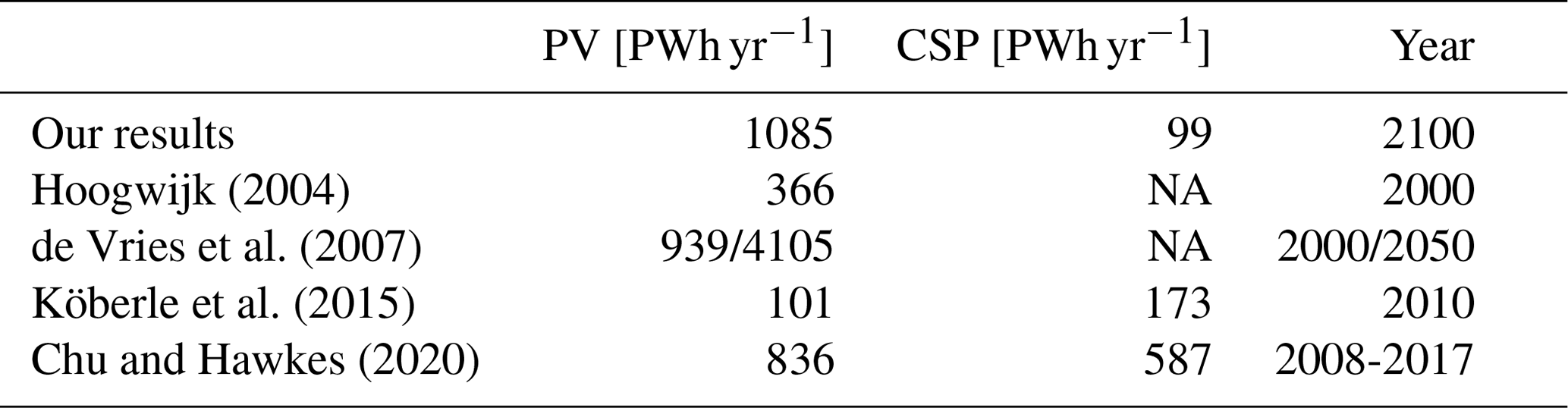
The total global energy potential of our analysis is broadly comparable with the large range given by existing studies that have looked at technical PV and CSP potential in the present or under climate change and provide their output in energy units (Hoogwijk, 2004; de Vries et al., 2007; Köberle et al., 2015; Chu and Hawkes, 2020) (Table 2). Our global PV potential is at the upper end, also due to the assumptions we make regarding the technological efficiency and socioeconomic circumstances at the end of the century.
Table 2Comparison of the PV and CSP potential with previous studies. Our results: SSP245. NA means not available.
The pattern and relative decrease in potential from greenhouse gases and other SSP-scenario-inherent climate active substances such as aerosols are broadly aligned with other studies that have analyzed PV and CSP potential under climate change (Crook et al., 2011; Wild et al., 2015; Gernaat et al., 2021; Zou et al., 2019; Scheele and Fiedler, 2023). For example, most of the abovementioned studies report the strongest signal of increase over Europe and East Asia. While our results do not point to a large increase in this area, we do see small increases or only little change over the same areas. The strongest negative signal in our results is over Tibet, which also broadly agrees with previous studies.
A major challenge with RE is the intermittent nature of the supply, rendering a high temporal resolution of output data a crucial aspect of any RE analysis. LEW is therefore a more relevant metric than 10-year average changes when it comes to energy production. Our low energy week metric suggests that the observed negative trend in 10-year averages for SAI with respect to SSP245 does not necessarily translate to an increase in extended periods of very low solar resources (Figs. 2a, 6d). While other studies have found only minor changes in the variability of solar PV energy production (Tobin et al., 2018; Jerez et al., 2015), our results demonstrate that, under geoengineering, the distribution of PV potential is more complex than a simple shift of the mean and standard deviation, and it might be important to look at high-temporal-resolution output.
The reduced productivity from geoengineering would be added on top of the burden of climate change (Figs. 7, S12). Meaning the failure to decarbonize early enough, which would render SRM unnecessary, makes it even more difficult to decarbonize later once SRM is deployed. Reduced solar RE productivity implies higher land use and financial requirements to generate the same amount of energy. This makes the technology less cost-efficient and less competitive against other sources of energy including fossil alternatives. If fossil alternatives were chosen over solar RE it could prolong the duration of the SRM deployment, implying higher risks and costs (Baur et al., 2023). If, on the other hand, solar RE is chosen despite the reduced productivity it would imply higher costs due to the greater amount of infrastructure required to generate energy. The results of this study should therefore be considered when constructing SRM scenarios that assume unchanged technical emission reduction potential under geoengineering.
Indeed, our analysis demonstrated how sensitive results are to assumptions that are independent of the change in resources, such as shifts in population and land use suitability (Figs. S4, S13). The same conclusion has been drawn by previous studies on RE (de Vries et al., 2007). Attempting to predict these variables with any degree of accuracy is, of course, likely to fail. By including area restriction and weighting in this study, but excluding any variation in these assumptions between the scenarios, we allowed the change in solar resources to be the driver of change while focusing on areas that are of interest for solar energy parks.
The main drivers of change in this study are the different types of radiation and temperature, and Fig. 3 shows their relative importance for PV potential between the scenarios. In reality, these variables are not independent and a breakdown to these single components may not be fully physically correct. However, it provides an idea of which differences between the scenarios are contributing to the total relative change in PV potential we see in Fig. 2. Figure 3 demonstrates how variation in cloud properties between the scenarios has a large effect on the result, especially the reduction in reflective cloud cover under SAI compared to SSP245 and SSP585. While other studies have found similar effects under SRM (Kuebbeler et al., 2012; Visioni et al., 2018), the parameterization of clouds in the climate models underlying their studies and our study is highly idealized and should be interpreted with caution. Furthermore, in CNRM-ESM2-1, since there is no interactive sulfur cycle and no stratospheric aerosol microphysics, SAI is represented by imposing a sulfate distribution that is calculated offline (Visioni et al., 2021).
Other more local SRM scenarios have been proposed, such as injecting aerosols solely over the Arctic (Jackson et al., 2015), which would have no direct effect on solar power output elsewhere. For a more in-depth discussion of the effects of different types of SRM on solar power output see Smith et al. (2017).
Finally, while solar renewable energy sources will likely play a role in the net-zero transition, they are only one part of it. Effects on other renewable sources such as wind, hydropower and bioenergy have to be considered to be able to draw a conclusion regarding the full effect of SRM on decarbonization, as well as an in-depth analysis of the effects on the carbon cycle. Furthermore, it may not be a question of a small reduction in solar RE productivity that is decisive, but rather whether the infrastructure for PV and CSP is actually developed on a significant scale. This depends on much more than just the technical potential. Production costs overall, the production costs and availability of alternatives, and policy incentives like subsidies and feed-in tariffs all play a major role when it comes to the choice and actual implementation of the energy generating system.
SRM is increasingly being considered as a tool to supplement traditional mitigation measures in reducing anthropogenic climate change. Currently, such simulations assume no physical link between SRM and the ability to decarbonize. Here, we assess one aspect of this coupling: whether SRM affects the potential to reduce emissions through its impacts on solar renewable energy.
We find that there is a significant decrease in PV and CSP potential under SAI compared to SSP245 in terms of both the number of weeks in a year with low solar resources and 10-year means. Compared to the baseline scenario SSP585, SAI appears to counterbalance some adverse effects in regions that see especially pronounced reductions in PV potential due to climate change, but overall, it worsens the trend. Regarding CSP, the increase in LEWs is of a similar magnitude to that of PV, but the 10-year average trends show twice the decline in potential for CSP than for PV.
The 10-year average trends in our results support existing theories (Murphy, 2009; Robock, 2008; Robock et al., 2009; Smith et al., 2017). However, our study adds a more comprehensive quantitative aspect to the discussion, especially with regards to the greater temporal resolution of our findings. Indeed, despite certain similarities in the trends of the 10-year averages and the weekly sums of hourly output (LEW), we note that there are regions, including some with high absolute potential such as desert areas, that show different developments under the 10-year mean changes and the weekly sums. When a tilt of the PV panel is taken into account, the reductions in potential under SAI become even more pronounced at higher latitudes. This is because the inclination maximizes the amount of direct radiation reaching the panel, while SAI alters the ratio of direct and diffuse radiation to increase the diffuse part. Therefore, when SAI is used, tilting the panels, while still advantageous in most latitudes, becomes less useful in maximizing radiative energy.
Since the principle of SAI is to cool temperatures by reducing incoming radiation, a reduction in potential was to be expected. However, there are two drivers we identify that change the outcome of PV in favor of SAI: changes in upper-tropospheric cloud cover compensate for a substantial amount of the decreased potential under SAI compared to both SSP245 and SSP585. As previous studies have suggested, this change in high-altitude cloud cover is mainly the result of temperature anomalies in the lower stratosphere due to the aerosols (Kuebbeler et al., 2012; Visioni et al., 2021, 2018). For SSP585, the reduction in regional temperatures is beneficial for photovoltaic panels, increasing their productivity, but disadvantageous for CSP.
Reducing emissions is one of the greatest challenges facing society today, and the record-breaking greenhouse gas emissions (Friedlingstein et al., 2022) indicate that we are still grappling with implementing effective mitigation strategies (UNEP, 2022). One of the key approaches that can take us closer to achieving net-zero emissions is the extensive implementation of sustainable energy sources such as PV and CSP (IPCC, 2011, 2022). Previous research has demonstrated (see, for example, Huber et al., 2016; Crook et al., 2011; Wild et al., 2015; Clarke et al., 2022; Scheele and Fiedler, 2023), and this study supports these findings, that climate change itself can already lead to a reduction in PV output in some regions. Here, we demonstrate that SRM would increase the challenge of mitigation further by reducing PV and CSP potential. This is another argument for early mitigation, as it suggests that failing to decarbonize early enough, which would render SRM unnecessary, makes it even more challenging to decarbonize later when SRM is implemented. And, since net-zero greenhouse gas emission is a crucial component of the buying time approach of SRM, this study's findings suggest that such an approach may be more challenging than previously recognized. This should be factored into the construction of SRM experiments that currently assume no coupling between SRM and mitigation. Of course, solar RE is only one part of the overall mitigation strategy and additional research is needed to establish a full picture of the linkage between SRM and decarbonization. This requires a complete and comprehensive assessment of other physical and ecological couplings between mitigation processes, SRM and carbon–climate feedbacks.
The code and post-processed data are available at https://doi.org/10.5281/zenodo.10658589 (Baur, 2024).
The supplement related to this article is available online at: https://doi.org/10.5194/esd-15-307-2024-supplement.
All authors conceptualized the study and SB carried it out. SB ran the simulations and prepared the paper with contributions from all authors.
At least one of the (co-)authors is a member of the editorial board of Earth System Dynamics. The peer-review process was guided by an independent editor, and the authors also have no other competing interests to declare.
Publisher's note: Copernicus Publications remains neutral with regard to jurisdictional claims made in the text, published maps, institutional affiliations, or any other geographical representation in this paper. While Copernicus Publications makes every effort to include appropriate place names, the final responsibility lies with the authors.
Susanne Baur is supported by CERFACS through the project MIRAGE. Benjamin M. Sanderson and Roland Séférian acknowledge funding by the European Union's Horizon 2020 (H2020) research and innovation program (ESM2025, 4C, and PROVIDE).
This research has been supported by CERFACS (MIRAGE) and the Horizon 2020 projects PROVIDE (grant no. 101003687), 4C (grant no. 821003), and ESM2025 (grant no. 101003536).
This paper was edited by Ben Kravitz and reviewed by two anonymous referees.
Angel, R.: Feasibility of cooling the Earth with a cloud of small spacecraft near the inner Lagrange point (L1), P. Natl. Acad. Sci. USA, 103, 17184–17189, https://doi.org/10.1073/pnas.0608163103, 2006.
Bartók, B., Wild, M., Folini, D., Lüthi, D., Kotlarski, S., Schär, C., Vautard, R., Jerez, S., and Imecs, Z.: Projected changes in surface solar radiation in CMIP5 global climate models and in EURO-CORDEX regional climate models for Europe, Clim. Dynam., 49, 2665–2683, https://doi.org/10.1007/s00382-016-3471-2, 2017.
Baur, S.: Data and code for journal article Solar Radiation Modification challenges decarbonisation with renewable solar energy, Zenodo [data set], https://doi.org/10.5281/zenodo.10658589, 2024.
Baur, S., Nauels, A., Nicholls, Z., Sanderson, B. M., and Schleussner, C.-F.: The deployment length of solar radiation modification: an interplay of mitigation, net-negative emissions and climate uncertainty, Earth Syst. Dynam., 14, 367–381, https://doi.org/10.5194/esd-14-367-2023, 2023.
Bazyomo, S. D. Y. B., Agnidé Lawin, E., Coulibaly, O., and Ouedraogo, A.: Forecasted Changes in West Africa Photovoltaic Energy Output by 2045, Climate, 4, 53, https://doi.org/10.3390/cli4040053, 2016.
Belaia, M., Moreno-Cruz, J. B., and Keith, D. W.: Optimal climate policy in 3D: mitigation, carbon removal, and solar geoengineering, Clim. Change Econ., 12, 2150008, https://doi.org/10.1142/S2010007821500081, 2021.
Bellamy, R., Chilvers, J., and Vaughan, N. E.: Deliberative Mapping of options for tackling climate change: Citizens and specialists “open up” appraisal of geoengineering, Public Underst. Sci., 25, 269–286, https://doi.org/10.1177/0963662514548628, 2016.
Boucher, O., Randall, D., Artaxo, P., Bretherton, C., Feingold, G., Forster, P., Kerminen, V. M., Kondo, Y., Liao, H., Lohmann, U., Rasch, P., Satheesh, S. K., Sherwood, S., Stevens, B., and Zhang, X. Y.: Clouds and aerosols, in: Climate Change 2013: The Physical Science Basis, Working Group I Contribution to the Fifth Assessment Report of the Intergovernmental Panel on Climate Change, edited by: Stocker, T. F., Qin, D., Plattner, G.-K., Tignor, M., Allen, S. K., Boschung, J., Nauels, A., Xia, Y., Bex, V., and Midgley, P. M., Cambridge University Press, Cambridge, United Kingdom and New York, NY, USA, 571–658, https://doi.org/10.1017/CBO9781107415324.016, 2013.
Budyko, M. I.: The future climate. Eos Trans, American Geophysical Union, 53, 868–874, https://doi.org/10.1029/EO053i010p00868, 1978.
Burns, E. T., Flegal, J. A., Keith, D. W., Mahajan, A., Tingley, D., and Wagner, G.: What do people think when they think about solar geoengineering? A review of empirical social science literature, and prospects for future research, Earth's Future, 4, 536–542, https://doi.org/10.1002/2016EF000461, 2016.
Chu, C.-T. and Hawkes, A. D.: A geographic information system-based global variable renewable potential assessment using spatially resolved simulation, Energy, 193, 116630, https://doi.org/10.1016/j.energy.2019.116630, 2020.
Clarke, L., Wei, Y.-M., De La Vega Navarro, A., Garg, A., Hahmann, A. N., Khennas, S., Azevedo, I. M. L., Löschel, A., Singh, A. K., Steg, L., Strbac, G., and Wada, K.: Energy Systems, in: IPCC, 2022: Climate Change 2022: Mitigation of Climate Change, Contribution of Working Group III to the Sixth Assessment Report of the Intergovernmental Panel on Climate Change, edited by: Shukla, P. R., Skea, J., Slade, R., Al Khourdajie, A., van Diemen, R., McCollum, D., Pathak, M., Some, S., Vyas, P., Fradera, R., Belkacemi, M., Hasija, A., Lisboa, G., Luz, S., and Malley, J., Cambridge University Press, Cambridge, UK and New York, NY, USA, https://doi.org/10.1017/9781009157926.008, 2022.
Crook, J. A., Jones, L. A., Forster, P. M., and Crook, R.: Climate change impacts on future photovoltaic and concentrated solar power energy output, Energ. Environ. Sci., 4, 3101–3109, https://doi.org/10.1039/c1ee01495a, 2011.
Crutzen, P. J.: Albedo enhancement by stratospheric sulfur injections: A contribution to resolve a policy dilemma?, Climatic Change, 77, 211–220, https://doi.org/10.1007/s10584-006-9101-y, 2006.
Cziczo, D. J., Wolf, M. J., Gasparini, B., Münch, S., and Lohmann, U.: Unanticipated Side Effects of Stratospheric Albedo Modification Proposals Due to Aerosol Composition and Phase, Sci. Rep., 9, 18825, https://doi.org/10.1038/s41598-019-53595-3, 2019.
de Vries, B. J. M., van Vuuren, D. P., and Hoogwijk, M. M.: Renewable energy sources: Their global potential for the first-half of the 21st century at a global level: An integrated approach, Energ. Policy, 35, 2590–2610, https://doi.org/10.1016/j.enpol.2006.09.002, 2007.
Doelman, J. C., Stehfest, E., Tabeau, A., Van Meijl, H., Lassaletta, L., Gernaat, D. E. H. J., Hermans, K., Harmsen, M., Daioglou, V., Biemans, H., Van Der Sluis, S., and Van Vuuren, D. P.: Exploring SSP land-use dynamics using the IMAGE model: Regional and gridded scenarios of land-use change and land-based climate change mitigation, Glob. Environ. Change, 48, 119–135, https://doi.org/10.1016/j.gloenvcha.2017.11.014, 2018.
Dubey, S., Sarvaiya, J. N., and Seshadri, B.: Temperature Dependent Photovoltaic (PV) Efficiency and Its Effect on PV Production in the World – A Review, Energy Proced., 33, 311–321, https://doi.org/10.1016/j.egypro.2013.05.072, 2013.
Dutta, R., Chanda, K., and Maity, R.: Future of solar energy potential in a changing climate across the world: A CMIP6 multi-model ensemble analysis, Renew. Energ., 188, 819–829, https://doi.org/10.1016/j.renene.2022.02.023, 2022.
Feron, S., Cordero, R. R., Damiani, A., and Jackson, R.: Climate change extremes and photovoltaic power output, Nat. Sustain., 4, 270–276, https://doi-org.insu.bib.cnrs.fr/10.1038/s41893-020-00643-w, 2021.
Fraunhofer ISE: Photovoltaics report, Fraunhofer Institute for Solar Energy Systems, https://www.ise.fraunhofer.de/content/dam/ise/de/documents/publications/studies/Photovoltaics-Report.pdf (last access: 10 June 2023), 2023.
Friedlingstein, P., O'Sullivan, M., Jones, M. W., Andrew, R. M., Gregor, L., Hauck, J., Le Quéré, C., Luijkx, I. T., Olsen, A., Peters, G. P., Peters, W., Pongratz, J., Schwingshackl, C., Sitch, S., Canadell, J. G., Ciais, P., Jackson, R. B., Alin, S. R., Alkama, R., Arneth, A., Arora, V. K., Bates, N. R., Becker, M., Bellouin, N., Bittig, H. C., Bopp, L., Chevallier, F., Chini, L. P., Cronin, M., Evans, W., Falk, S., Feely, R. A., Gasser, T., Gehlen, M., Gkritzalis, T., Gloege, L., Grassi, G., Gruber, N., Gürses, Ö., Harris, I., Hefner, M., Houghton, R. A., Hurtt, G. C., Iida, Y., Ilyina, T., Jain, A. K., Jersild, A., Kadono, K., Kato, E., Kennedy, D., Klein Goldewijk, K., Knauer, J., Korsbakken, J. I., Landschützer, P., Lefèvre, N., Lindsay, K., Liu, J., Liu, Z., Marland, G., Mayot, N., McGrath, M. J., Metzl, N., Monacci, N. M., Munro, D. R., Nakaoka, S.-I., Niwa, Y., O'Brien, K., Ono, T., Palmer, P. I., Pan, N., Pierrot, D., Pocock, K., Poulter, B., Resplandy, L., Robertson, E., Rödenbeck, C., Rodriguez, C., Rosan, T. M., Schwinger, J., Séférian, R., Shutler, J. D., Skjelvan, I., Steinhoff, T., Sun, Q., Sutton, A. J., Sweeney, C., Takao, S., Tanhua, T., Tans, P. P., Tian, X., Tian, H., Tilbrook, B., Tsujino, H., Tubiello, F., van der Werf, G. R., Walker, A. P., Wanninkhof, R., Whitehead, C., Willstrand Wranne, A., Wright, R., Yuan, W., Yue, C., Yue, X., Zaehle, S., Zeng, J., and Zheng, B.: Global Carbon Budget 2022, Earth Syst. Sci. Data, 14, 4811–4900, https://doi.org/10.5194/essd-14-4811-2022, 2022.
Gernaat, D. E. H. J., de Boer, H. S., Daioglou, V., Yalew, S. G., Müller, C., and van Vuuren, D. P.: Climate change impacts on renewable energy supply, Nat. Clim. Change, 11, 119–125, https://doi.org/10.1038/s41558-020-00949-9, 2021.
Hernandez, R. R., Hoffacker, M. K., Murphy-Mariscal, M. L., Wu, G. C., and Allen, M. F.: Solar energy development impacts on land cover change and protected areas, P. Natl. Acad. Sci. USA, 112, 13579–13584, https://doi.org/10.1073/pnas.1517656112, 2015.
Hoogwijk, M. M.: On the global and regional potential of renewable energy sources = Over het mondiale en regionale potentieel van hernieuwbare energiebronnen, Universiteit Utrecht, Faculteit Scheikunde, Utrecht, ISBN: 9789039336403, 2004.
Huber, I., Bugliaro, L., Ponater, M., Garny, H., Emde, C., and Mayer, B.: Do climate models project changes in solar resources?, Sol. Energy, 129, 65–84, https://doi.org/10.1016/j.solener.2015.12.016, 2016.
Irvine, P. J., Kravitz, B., Lawrence, M. G., and Muri, H.: An overview of the Earth system science of solar geoengineering, Wiley Interdisciplinary Reviews, Climate Change, 7, 815–833, https://doi.org/10.1002/wcc.423, 2016.
Iturbide, M., Gutiérrez, J. M., Alves, L. M., Bedia, J., Cerezo-Mota, R., Cimadevilla, E., Cofiño, A. S., Di Luca, A., Faria, S. H., Gorodetskaya, I. V., Hauser, M., Herrera, S., Hennessy, K., Hewitt, H. T., Jones, R. G., Krakovska, S., Manzanas, R., Martínez-Castro, D., Narisma, G. T., Nurhati, I. S., Pinto, I., Seneviratne, S. I., van den Hurk, B., and Vera, C. S.: An update of IPCC climate reference regions for subcontinental analysis of climate model data: definition and aggregated datasets, Earth Syst. Sci. Data, 12, 2959–2970, https://doi.org/10.5194/essd-12-2959-2020, 2020.
IPCC (Intergovernmental Panel on Climate Change): Renewable Energy Sources and Climate Change Mitigation, edited by: Edenhofer, O., Pichs-Madruga, R., Sokona, Y., Seyboth, K., Matschoss, P., Kadner, S., Zwickel, T., Eickemeier, P., Hansen, G., Schloemer, S., von Stechow, C., Cambridge University Press, Cambridge, United Kingdom and New York, NY, USA, 0–1075, https://doi.org/10.1017/CBO9781139151153, 2011.
IPCC (Intergovernmental Panel on Climate Change): Climate Change 2022: Mitigation of Climate Change, Contribution of Working Group III to the Sixth Assessment Report of the Intergovernmental Panel on Climate Change, edited by: Shukla, P. R., Skea, J., Slade, R., Al Khourdajie, A., van Diemen, R., McCollum, D., Pathak, M., Some, S., Vyas, P., Fradera, R., Belkacemi, M., Hasija, A., Lisboa, G., Luz, S., and Malley, J., Cambridge University Press, Cambridge, UK and New York, NY, USA, https://doi.org/10.1017/9781009157926, 2022.
IUCN (International Union for Conservation of Nature): The World Database on Protected Areas (WDPA), https://www.protectedplanet.net/en/themaPc-areas/wdpa?tab=WDPA (last access: 13 March 2023), 2023.
Jackson, L. S., Crook, J. A., Jarvis, A., Leedal, D., Ridgwell, A., Vaughan, N., and Forster, P. M.: Assessing the controllability of Arctic sea ice extent by sulfate aerosol geoengineering, Geophys. Res. Lett., 42, 1223–1231, https://doi.org/10.1002/2014GL062240, 2015.
Jerez, S., Tobin, I., Vautard, R., Montávez, J. P., López-Romero, J. M., Thais, F., Bartok, B., Christensen, O. B., Colette, A., Déqué, M., Nikulin, G., Kotlarski, S., Van Meijgaard, E., Teichmann, C., and Wild, M.: The impact of climate change on photovoltaic power generation in Europe, Nat. Commun., 6, 10014, https://doi.org/10.1038/ncomms10014, 2015.
Keith, D. W.: Geoengineering the climate: History and Prospect, Annu. Rev. Energy Environ., 25, 245–84, 2000.
Khan, M. S., Ramli, M. A. M., Sindi, H. F., Hidayat, T., and Bouchekara, H. R. E. H.: Estimation of Solar Radiation on a PV Panel Surface with an Optimal Tilt Angle Using Electric Charged Particles Optimization, Electronics, 11, 2056, https://doi.org/10.3390/electronics11132056, 2022.
Köberle, A. C., Gernaat, D. E. H. J., and van Vuuren, D. P.: Assessing current and future techno-economic potential of concentrated solar power and photovoltaic electricity generation, Energy, 89, 739–756, https://doi.org/10.1016/j.energy.2015.05.145, 2015.
Kravitz, B., Robock, A., Tilmes, S., Boucher, O., English, J. M., Irvine, P. J., Jones, A., Lawrence, M. G., MacCracken, M., Muri, H., Moore, J. C., Niemeier, U., Phipps, S. J., Sillmann, J., Storelvmo, T., Wang, H., and Watanabe, S.: The Geoengineering Model Intercomparison Project Phase 6 (GeoMIP6): Simulation design and preliminary results, Geosci. Model Dev., 8, 3379–3392, https://doi.org/10.5194/gmd-8-3379-2015, 2015.
Kuebbeler, M., Lohmann, U., and Feichter, J.: Effects of stratospheric sulfate aerosol geo-engineering on cirrus clouds: effects of geo-engineering on cirrus, Geophys. Res. Lett., 39, L23803, https://doi.org/10.1029/2012GL053797, 2012.
Latham, J.: Control of global warming, Nature, 347, 339–340, 1990.
Mahdavi, A., Farhadi, M., Gorji-Bandpy, M., and Mahmoudi, A.: A review of passive cooling of photovoltaic devices, Cleaner Eng. Technol., 11, 100579, https://doi.org/10.1016/j.clet.2022.100579, 2022.
McLaren, D.: Mitigation deterrence and the “moral hazard” of solar radiation management, Earth's Future, 4, 596–602, https://doi.org/10.1002/2016EF000445, 2016.
Merk, C., Pönitzsch, G., and Rehdanz, K.: Knowledge about aerosol injection does not reduce individual mitigation efforts, Environ. Res. Lett., 11, 054009, https://doi.org/10.1088/1748-9326/11/5/054009, 2016.
Mitchell, D. L. and Finnegan, W.: Modification of cirrus clouds to reduce global warming, Environ. Res. Lett., 4, 045102, https://doi.org/10.1088/1748-9326/4/4/045102, 2009.
Moreno-Cruz, J.: Mitigation and the geoengineering threat, Resour. Energ. Econ., 41, 248–263, https://doi.org/10.1016/j.reseneeco.2015.06.001, 2015.
Murphy, D. M.: Effect of Stratospheric Aerosols on Direct Sunlight and Implications for Concentrating Solar Power, Environ. Sci. Technol., 43, 2784–2786, https://doi.org/10.1021/es802206b, 2009.
NREL (National Renewable Energy Laboratory): Best Research-Cell Efficiency Chart, National Renewable Energy Laboratory, https://www.nrel.gov/pv/cell-efficiency.html (last access: August 2023), 2023.
O'Neill, B. C., Tebaldi, C., Van Vuuren, D. P., Eyring, V., Friedlingstein, P., Hurtt, G., Knutti, R., Kriegler, E., Lamarque, J.-F., Lowe, J., Meehl, G. A., Moss, R., Riahi, K., and Sanderson, B. M.: The Scenario Model Intercomparison Project (ScenarioMIP) for CMIP6, Geosci. Model Dev., 9, 3461–3482, https://doi.org/10.5194/gmd-9-3461-2016, 2016.
Parretta, A., Yakubu, H., Ferrazza, F., Altermatt, P. P., Green, M. A., and Zhao, J.: Optical loss of photovoltaic modules under diffuse light, Sol. Energ. Mat. Sol. C., 75, 497–505, https://doi.org/10.1016/S0927-0248(02)00199-X, 2003.
Radziemska, E.: The effect of temperature on the power drop in crystalline silicon solar cells, Renew. Energ., 28, 1–12, 2003.
Rahman, M. M., Hasanuzzaman, M., and Rahim, N. A.: Effects of various parameters on PV-module power and efficiency, Energ. Convers. Manage., 103, 348–358, https://doi.org/10.1016/j.enconman.2015.06.067, 2015.
Robock, A.: 20 reasons why geoengineering may be a bad idea, B. Atom. Sci., 64, 14–59, https://doi.org/10.1080/00963402.2008.11461140, 2008.
Robock, A., Marquardt, A., Kravitz, B., and Stenchikov, G.: Benefits, risks, and costs of stratospheric geoengineering, Geophys. Res. Lett., 36, https://doi.org/10.1029/2009GL039209, 2009.
Sawadogo, W., Reboita, M. S., Faye, A., da Rocha, R. P., Odoulami, R. C., Olusegun, C. F., Adeniyi, M. O., Abiodun, B. J., Sylla, M. B., Diallo, I., Coppola, E., and Giorgi, F.: Current and future potential of solar and wind energy over Africa using the RegCM4 CORDEX-CORE ensemble, Clim. Dynam., 57, 1647–1672, https://doi.org/10.1007/s00382-020-05377-1, 2021.
Schaeffer, R., Szklo, A. S., Pereira de Lucena, A. F., Moreira Cesar Borba, B. S., Pupo Nogueira, L. P., Fleming, F. P., Troccoli, A., Harrison, M., and Boulahya, M. S.: Energy sector vulnerability to climate change: A review, Energy, 38, 1–12, https://doi.org/10.1016/j.energy.2011.11.056, 2012.
Scheele, R. C. and Fiedler, S.: What drives historical and future changes in photovoltaic power production from the perspective of global warming?, Environ. Res. Lett., 19, 014030, https://doi.org/10.1088/1748-9326/ad10d6, 2023.
Séférian, R., Nabat, P., Michou, M., Saint-Martin, D., Voldoire, A., Colin, J., Decharme, B., Delire, C., Berthet, S., Chevallier, M., Sénési, S., Franchisteguy, L., Vial, J., Mallet, M., Joetzjer, E., Geoffroy, O., Guérémy, J.-F., Moine, M.-P., Msadek, R., Ribes, A., Rocher, M., Roehrig, R., Salas-y-Mélia, D., Sanchez, E., Terray, L., Valcke, S., Waldman, R., Aumont, O., Bopp, L., Deshayes, J., Éthé, C., and Madec, G.: Evaluation of CNRM Earth System Model, CNRM-ESM2-1: Role of Earth System Processes in Present-Day and Future Climate, J. Adv. Model. Earth Syst., 11, 4182–4227, https://doi.org/10.1029/2019MS001791, 2019.
Smith, C. J., Crook, J. A., Crook, R., Jackson, L. S., Osprey, S. M., and Forster, P. M.: Impacts of stratospheric sulfate geoengineering on global solar photovoltaic and concentrating solar power resource, J. Appl. Meteorol. Climatol., 56, 1483–1497, https://doi.org/10.1175/JAMC-D-16-0298.1, 2017.
Stehfest, E., Van Vuuren, D., Kram, T., Bouwman, L., Alkemade, R., Bakkenes, M., Biemans, H., Bouwman, A., Den Elzen, M., Janse, J., Lucas, P., Van Minnen, J., Müller, C., and Prins, A.: Integrated Assessment of Global Environmental Change with IMAGE 3.0. Model Description and Policy Applications, Netherlands Environmental Assessment Agency (The Hague), ISBN: 978-94-91506-71-0, 2014.
Tilmes, S., Mills, M. J., Niemeier, U., Schmidt, H., Robock, A., Kravitz, B., Lamarque, J.-F., Pitari, G., and English, J. M.: A new Geoengineering Model Intercomparison Project (GeoMIP) experiment designed for climate and chemistry models, Geosci. Model Dev., 8, 43–49, https://doi.org/10.5194/gmd-8-43-2015, 2015.
Tobin, I., Greuell, W., Jerez, S., Ludwig, F., Vautard, R., Van Vliet, M. T. H., and Breón, F. M.: Vulnerabilities and resilience of European power generation to 1.5 °C, 2 °C and 3 °C warming, Environ. Res. Lett., 13, 044024, https://doi.org/10.1088/1748-9326/aab211, 2018.
Trieb, F., Schillings, C., O'Sullivan, M., Pregger, T., and Hoyer-Klick, C.: Global Potential of Concentrating Solar Power, 11, SolarPaces Conference Berlin, September 2009, 2009.
UNEP (United Nations Environment Programme): Emissions Gap Report 2022: The Closing Window – Climate crisis calls for rapid transformation of societies, Nairobi, https://www.unep.org/emissions-gap-report-2022 (last access: 17 September 2023), 2022.
Visioni, D., Pitari, G., Di Genova, G., Tilmes, S., and Cionni, I.: Upper tropospheric ice sensitivity to sulfate geoengineering, Atmos. Chem. Phys., 18, 14867–14887, https://doi.org/10.5194/acp-18-14867-2018, 2018.
Visioni, D., MacMartin, D. G., and Kravitz, B.: Is Turning Down the Sun a Good Proxy for Stratospheric Sulfate Geoengineering?, J. Geophys. Res.-Atmos., 126, e2020JD033952, https://doi.org/10.1029/2020JD033952, 2021.
Wibeck, V., Hansson, A., and Anshelm, J.: Questioning the technological fix to climate change – Lay sense-making of geoengineering in Sweden, Energ. Res. Soc. Sci., 7, 23–30, https://doi.org/10.1016/j.erss.2015.03.001, 2015.
Wild, M., Folini, D., Henschel, F., Fischer, N., and Müller, B.: Projections of long-term changes in solar radiation based on CMIP5 climate models and their influence on energy yields of photovoltaic systems, Sol. Energy, 116, 12–24, https://doi.org/10.1016/j.solener.2015.03.039, 2015.
Zou, L., Wang, L., Li, J., Lu, Y., Gong, W., and Niu, Y.: Global surface solar radiation and photovoltaic power from Coupled Model Intercomparison Project Phase 5 climate models, J. Clean. Prod., 224, 304–324, https://doi.org/10.1016/j.jclepro.2019.03.268, 2019.