the Creative Commons Attribution 4.0 License.
the Creative Commons Attribution 4.0 License.
 | 18 Mar 2024
Possible role of anthropogenic climate change in the record-breaking 2020 Lake Victoria levels and floods
Inne Vanderkelen
Friederike E. L. Otto
Clair Barnes
Lucy Temple
Mary Akurut
Philippe Bally
Nicole P. M. van Lipzig
Wim Thiery
Heavy rainfall in eastern Africa between late 2019 and mid 2020 caused devastating floods and landslides throughout the region. These rains drove the levels of Lake Victoria to a record-breaking maximum in the second half of May 2020. The combination of high lake levels, consequent shoreline flooding, and flooding of tributary rivers caused hundreds of casualties and damage to housing, agriculture, and infrastructure in the riparian countries of Uganda, Kenya, and Tanzania. Media and government reports linked the heavy precipitation and floods to anthropogenic climate change, but a formal scientific attribution study has not been carried out so far. In this study, we characterize the spatial extent and impacts of the floods in the Lake Victoria basin and then investigate to what extent human-induced climate change influenced the probability and magnitude of the record-breaking lake levels and associated flooding by applying a multi-model extreme event attribution methodology. Using remote-sensing-based flood mapping tools, we find that more than 29 000 people living within a 50 km radius of the lake shorelines were affected by floods between April and July 2020. Precipitation in the basin was the highest recorded in at least 3 decades, causing lake levels to rise by 1.21 m between late 2019 and mid 2020. The flood, defined as a 6-month rise in lake levels as extreme as that observed in the lead-up to May 2020, is estimated to be a 63-year event in the current climate. Based on observations and climate model simulations, the best estimate is that the event has become more likely by a factor of 1.8 in the current climate compared to a pre-industrial climate and that in the absence of anthropogenic climate change an event with the same return period would have led lake levels to rise by 7 cm less than observed. Nonetheless, uncertainties in the attribution statement are relatively large due to large natural variability and include the possibility of no observed attributable change in the probability of the event (probability ratio, 95 % confidence interval 0.8–15.8) or in the magnitude of lake level rise during an event with the same return period (magnitude change, 95 % confidence interval 0–14 cm). In addition to anthropogenic climate change, other possible drivers of the floods and their impacts include human land and water management, the exposure and vulnerability of settlements and economic activities located in flood-prone areas, and modes of climate variability that modulate seasonal precipitation. The attribution statement could be strengthened by using a larger number of climate model simulations, as well as by quantitatively accounting for non-meteorological drivers of the flood and potential unforced modes of climate variability. By disentangling the role of anthropogenic climate change and natural variability in the high-impact 2020 floods in the Lake Victoria basin, this paper contributes to a better understanding of changing hydrometeorological extremes in eastern Africa and the African Great Lakes region.
- Article
(18220 KB) - Full-text XML
-
Supplement
(438 KB) - BibTeX
- EndNote


Between late 2019 and mid 2020, eastern Africa experienced heavy rainfall that led to flooding and landslides across the region, displacing over a million people according to some sources1 and causing hundreds of casualties2. In 2019, the rainy season of October, November, and December (OND, known as the short rains) was one of the heaviest seen in the region in the last 3 decades (Wainwright et al., 2021a). Wet conditions compared to the climatological average continued into the 2020 rainy season of March, April, and May (MAM, known as the long rains), causing additional floods and landslides in 2020. The heavy rains aggravated one of the most serious desert locust outbreaks the region has seen in decades. Moreover, this occurred concurrently with the COVID-19 pandemic, setting the stage for a perfect storm of compounding impacts on people's lives and livelihoods3.
Lake Victoria, the second largest freshwater lake in the world, shared between Kenya, Uganda, and Tanzania, also received above-average precipitation. The lake's levels began to rise in late September 2019 until reaching record-breaking levels in mid May 2020, thereby exceeding the previous maximum levels measured in 1964 (Fig. 1). From April 2020, floods were reported in the Lake Victoria basin, both along the lake shores and in the floodplains of rivers flowing into the lake. For example, in Kenya, an estimated 40 000 people were displaced when the Nzoia River burst its banks in early May 20204. In Tanzania, in the Kagera and Mara basins, 5000 people were displaced due to flash and river floods between March and May 20205. In Uganda, lake shoreline flooding affected the cities of Entebbe and Kampala6, and over 3800 people were displaced from the lake islands of the Mayuge District7. Some media8 and government reports (e.g. Government of Kenya and UNDP, 2021) linked the heavy precipitation and floods to anthropogenic climate change, but the connection has not been scientifically investigated with extreme event attribution methods so far.
This study aims to investigate whether human-induced climate change contributed to the probability and magnitude of the flooding and record-breaking lake levels observed in 2020 in the Lake Victoria basin by following an established protocol for probabilistic extreme event attribution (Philip et al., 2020). Event attribution studies classically define an extreme event based on its meteorological driver. For example, previous attribution studies have mostly defined flood events based on accumulated precipitation amounts (e.g. Otto et al., 2018b; Philip et al., 2018a). Some notable exceptions have extended the analysis, defining the event based on hydrological variables instead (e.g. Pall et al., 2011; Schaller et al., 2016; Philip et al., 2019). Here, we expand on the classical framework by focusing on an impact-relevant variable, namely by defining the flood event based on lake levels.
The eastern Africa region is comparatively under-studied in relation to flood attribution, with most previous studies having focused on drought events, generally finding either no attributable role of anthropogenic climate change (e.g. Uhe et al., 2018; Philip et al., 2018b; Otto et al., 2018a; Kew et al., 2021) or a significant increase in the likelihood of drought events (e.g. Funk et al., 2016, 2019; Marthews et al., 2019; Kimutai et al., 2023), depending on the specific location, framing, and variable being attributed in the study. One study has analysed the flood-inducing heavy long rains seasons that occurred in Kenya in 2012, 2016, and 2018, finding no significant trend attributable to human-induced climate change (Kimutai et al., 2022). To our knowledge, this study is the first to use water balance or hydrological modelling to attribute flood events in the region.
To study the floods, we follow a three-step methodology. First, we estimate the flooded area and number of people impacted through a remote sensing analysis. We then use a water balance model for Lake Victoria to reconstruct historical lake levels and identify which water balance terms drove the 2020 flooding. Finally, we use the water balance model as an impact model within a probabilistic extreme event attribution framework to detect the role played by anthropogenic climate change on the observed rapid rise in lake levels. We compare our estimate of impact with emergency databases and media and government reports and frame the results from statistical attribution within the context of previous research on changing hydro-climatic conditions in the region and on other possible drivers of the floods.
1.1 Event definition
In this study, we focus on lake levels to define the 2020 flood event, as (i) lake levels are closer to flooding impacts compared to accumulated precipitation amounts, which are the proximate meteorological driver of the event, and (ii) the lake levels were record-breaking in 2020, making headline statements in media reports and raising public interest. Furthermore, since tributary river floods are aggravated by backwater effects when lake levels are high (WMO et al., 2004), we assume that (iii) the lake levels are a proxy for the flooding of tributary rivers. Finally, (iv) the long historical time series of lake level measurements allows for more robust statistical attribution statements.
In the 8 months between September 2019 and May 2020, lake levels rose by 1.44 m, reaching the record-breaking level of 13.46 m measured in situ on 17 May 2020 (Fig. 1). Of this rise, 84 % (1.21 m) occurred in the 6 months between November 2019 and May 2020. We define the 2020 flood event as a 6-month rate of change in levels as extreme as that observed in the lead-up to May 2020. By using the rate of change in lake levels instead of absolute lake levels, we focus on signals in seasonal and year-to-year variability and limit the influence of decadal trends. The choice of a 6-month time window reflects the balance between, on the one hand, limiting the influence of decadal trends, and, on the other hand, defining the event in a way that represents the slow accumulated response of lake levels to seasonal accumulations of precipitation (Khaki and Awange, 2021). We test the sensitivity to these choices in Sect. 3.3 and Appendix Sect. B3.
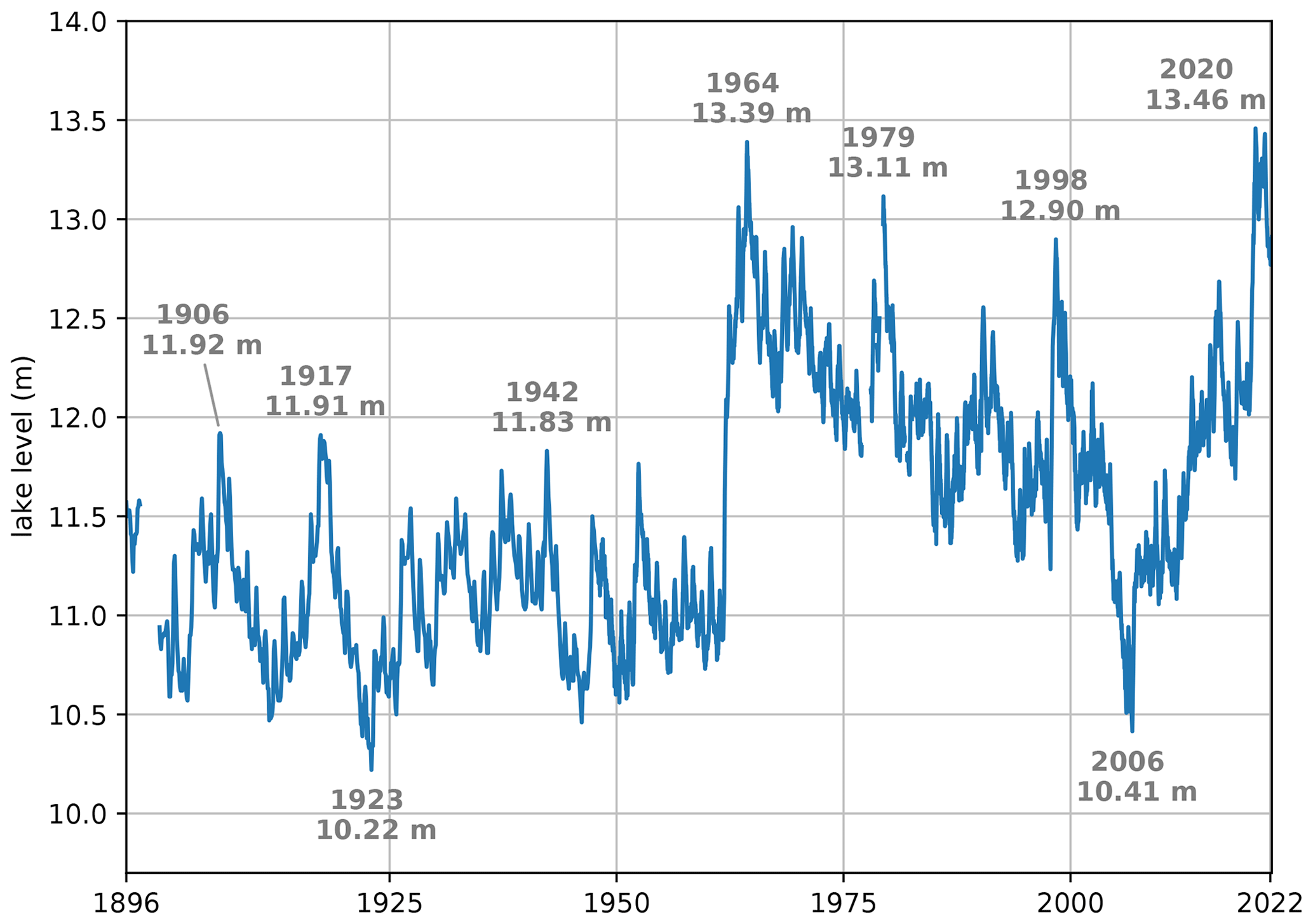
Figure 1Lake Victoria levels (1896–2022) with high and low peaks labelled. The time series is reconstructed based on monthly in situ measurements from the UK Centre for Ecology and Hydrology (UKCEH, 1896–1948), daily in situ measurements from the WMO Hydrometeorological Survey (1948–1992), and satellite-derived 10-daily measurements from the Database for Hydrological Time Series of Inland Waters (DAHITI) (in m a.s.l.) converted to in situ (1992–2022).
1.2 Previous variations in lake levels
Lake level fluctuations are the result of the lake's water balance, which consists of precipitation on the lake surface (∼ 70 %) and inflow from tributary rivers (∼ 20 %–30 %) as input terms and evaporation from the lake surface (∼ 70 %–80 %) and outflow from the Nalubaale dam complex in Jinja (∼ 20 %–30 %) as output terms (Vanderkelen et al., 2018a). Lake precipitation and inflow control seasonal and interannual lake level variability, as evaporation and outflow are characterized by lower variability (Sene et al., 2021). Outflow from the lake is managed as a function of lake levels following the Agreed Curve (Sene, 2000, see Sect. 2.1.2).
Lake Victoria's levels have varied by over 3.2 m since the beginning of instrumental measurements in the late 19th century (Fig. 1). Seasonal variations in lake levels are generally small compared to interannual variations (Sene et al., 2021). In 1954, the first dam of the Nalubaale dam complex, which controls the lake outflow and is located near Jinja, Uganda, was completed (Sutcliffe and Petersen, 2007). Subsequently, a remarkable spike in lake levels occurred in the early 1960s, which has been attributed to an increase in eastern African precipitation that affected the levels of multiple lakes in the African Great Lakes region (Sene et al., 2021; Kite, 1981). A period of generally declining lake levels occurred from the mid 1960s to the mid 2000s, which was linked to a combination of low precipitation and excessive release from the lake's dam (Vanderkelen et al., 2018b; Sene et al., 2021). From then on, levels show a generally positive trend and increased by approximately 3 m between 2006 and 2020. A particularly rapid increase in levels occurred between late 2019 and mid 2020, and the levels measured in May 2020 broke the previous 1964 record by approximately 7 cm.
1.3 Precipitation variability, extremes, and model representation in eastern Africa
The Lake Victoria basin is located in the African Great Lakes region and characterized by a bimodal rainfall distribution pattern, with rains concentrated in the “long rains” season in March, April, and May and the “short rains” season in October, November, and December (Thiery et al., 2015; Vanderkelen et al., 2018a). The region exhibits strong interannual variability in precipitation, influenced by the El Niño–Southern Oscillation (ENSO) and the Indian Ocean Dipole (IOD) (Nicholson, 2017; Ummenhofer et al., 2009; Black, 2005; Palmer et al., 2023). The spatial distribution of precipitation in the basin is influenced by topography and the presence of the lake, with high accumulated precipitation amounts and a tendency for hazardous night-time thunderstorms over the lake surface (Thiery et al., 2016; Van de Walle et al., 2020). The heavy 2019 short rains rainy season in eastern Africa was linked to a strong positive IOD event (Wainwright et al., 2021a; Nicholson et al., 2022; Khaki and Awange, 2021), with anomalies in sea surface temperatures leading to weakened westerlies in the Indian Ocean and wetter than usual conditions in eastern Africa (Wainwright et al., 2021a; Black, 2005; Nicholson, 2017).
Global and regional climate models generally project an increase in average annual precipitation amounts over eastern Africa with climate change (e.g. Rowell et al., 2015; Akurut et al., 2014; Dunning et al., 2018; Souverijns et al., 2016; Olaka et al., 2019), particularly during the short rains (Palmer et al., 2023), as well as an increasing frequency of extreme positive IOD events (Cai et al., 2014, 2018). At the same time, there is evidence of biases in coupled climate models in representing seasonal precipitation in eastern Africa, particularly with respect to the long rains (see Discussion Sect. 4; Wainwright et al., 2019; Palmer et al., 2023; Ayugi et al., 2021). Nonetheless, since our study is not restricted to the long rains season, and since coupled global climate models (GCMs) remain invaluable tools to simulate factual and counterfactual (i.e. in the absence of anthropogenic climate change) climate conditions in the most complete way (Otto, 2017), extreme event attribution studies of hydrological changes in the region using coupled GCMs and other modelling setups can still contribute to improving our understanding of ongoing changes in the region (e.g. Philip et al., 2018b; Kew et al., 2021; Kimutai et al., 2022, 2023).
2.1 Data
2.1.1 Remote sensing imagery and population data
The spatial extent of the flooding in the Lake Victoria Basin is estimated by applying the HASARD flood detection algorithm (Sect. 2.2.1) to remote sensing imagery from the Sentinel-1 and Sentinel-2 missions of the Copernicus programme of the European Union. We analyse Sentinel-1 level 1 ground range-detected C-band synthetic aperture radar (SAR) over a 3-month window from early April to the end of June 2020 (5 April 2020–1 July 2020). This period is centred around 17 May 2020, when lake levels reached their record high, and spans the period of reported flooding impacts in media reports and emergency and disaster databases, such as the Emergency Events Database (EM-DAT) of the Centre for Research on the Epidemiology of Disasters (CRED). SAR imagery is well suited for flood detection, as it provides imagery throughout day and night in all weather conditions (Chini et al., 2020). The imagery, collected in Interferometric Wide Swath mode, has a spatial resolution of 5 by 20 m, and a combined cycle revisit time of 6 d at the latitude of Lake Victoria. In addition, the algorithm uses optical imagery from the Sentinel-2 mission for the same period and spatial extent as a secondary data source. Sentinel-1 and Sentinel-2 imagery is accessed and processed through the Geohazards Exploitation Platform (GEP) operated by Terradue and developed in the framework of the European Space Agency Thematic Exploitation Platforms (TEP) and the Web Advanced Space Developer Interface (WASDI) operated by WASDI (Luxembourg) with Earth observation (EO) services developed by LIST (Luxembourg). To correct for permanent waterbodies that are erroneously identified as flooded, we use the waterbody mask of the Copernicus Global Digital Elevation Model at 30 m resolution (COPDEM GLO-30; Fahrland et al., 2020).
High-resolution gridded population data are obtained from the WorldPop database for Kenya, Uganda, and Tanzania (Appendix Fig. C1). The dataset is based on 2020 census data from the three countries, disaggregated based on building footprints and ancillary geospatial datasets (top-down constrained data, Stevens et al., 2015; WorldPop, 2018), and has a spatial resolution of 3 arcsec (approximately 100 m at the Equator).
2.1.2 Lake level observations
A time series of lake level measurements from 1896–2021 is assembled from different sources. For the period 1 January 1948–1 August 1996, daily measurements recorded in situ at Jinja are available from the World Meteorological Organization (WMO) Hydrometeorological Survey (hereafter Hydromet; WMO-UNDP, 1974). The data gaps in the years 1977 (whole year), 1978 (9–31 August), 1979 (15–31 December), 1979 (1 January–9 May), 1981 (1 October–31 December), and 1982 (15 July–2 December) are filled through linear interpolation. From 27 September 1992 to 2021, satellite-derived measurements are obtained from the Database for Hydrological Time Series of Inland Waters (DAHITI) at an approximately 10-daily resolution. In situ Hydromet measurements are converted to absolute levels in metres above sea level with a geoid datum and are corrected to match satellite-derived DAHITI measurements by adding the remaining average difference between the two datasets for the overlapping period (1992–1996), as in Vanderkelen et al. (2018a). The total resulting geoid correction applied to the Hydromet time series to obtain absolute lake levels in metres above sea level is 1123.32 m.
Furthermore, the near-daily in situ lake level measurements are supplemented by a monthly time series from the UK Centre for Ecology and Hydrology (Sene et al., 2021; Sutcliffe and Petersen, 2007) for the period 1896–1948. We thus create a single 127-year lake level time series, which we use in the observational attribution analysis. We test the attribution statement for sensitivity to the different temporal resolutions of the older and more recent data and find a similar attribution signal when the data are artificially upscaled to monthly resolution.
2.1.3 Observed global mean temperatures
As a measure of anthropogenic climate change, we use a time series of global mean surface temperature (GMST) obtained from the National Aeronautics and Space Administration (NASA) Goddard Institute for Space Science (GISS) surface temperature analysis (GISTEMP; Hansen et al., 2010; Lenssen et al., 2019). The time series is expressed as an anomaly relative to the 1951–1980 global average. A 4-year running mean low-pass filter is applied to remove higher-frequency variability and signals linked to ENSO, as recommended in Philip et al. (2020).
2.1.4 Observational data for water balance terms
The water balance of Lake Victoria is modelled using an updated version of the model described in Vanderkelen et al. (2018a) using observational data for the period 1983–2020. As input data, the water balance model (WBM) employs daily data for precipitation over the lake and basin and lake evaporation and a time series of dam outflow.
Daily observational gridded precipitation data are obtained for 1983–2020 from the satellite-derived dataset Precipitation Estimation from Remotely Sensed Information using Artificial Neural Networks – Climate Data Record (PERSIANN-CDR; Ashouri et al., 2015) at a 0.25° spatial resolution (approximately 28 km at the Equator). This dataset has been shown to perform better than other satellite-derived and reanalysis-based products in the study area (Nicholson and Klotter, 2021). Missing data occur mostly in the first decades of the dataset (419 total missing days spread across 32 years, of which 95 % are between 1983 and 1999 and 5 % are between 2007 and 2014, Appendix Fig. C2), with a third of the missing days concentrated in the 2-year period 1983–1984, and thus we restrict our analysis of the precipitation anomaly to the period 1985–2020 (see Appendix Sect. B1).
Daily inflow, evaporation from the lake surface, and outflow from the dam are calculated as in Vanderkelen et al. (2018a). Inflow is estimated from precipitation based on land use, soil type, soil hydrological characteristics, and antecedent moisture conditions using the USDA curve number method (USDA-SCS, 2004, see further details in Appendix Sect. B2). Evaporation from the lake surface is estimated based on the latent heat flux term simulated by the regional climate model COSMO-CLM2 forced with ERA5 reanalysis data over the African Great Lakes region for the period 1996–2008 (Thiery et al., 2015, 2016). The latent heat flux is converted to an evaporated water amount by dividing the flux term by the latent heat of vaporization of water, held constant at 2.5 × 10⁶ J kg−1. A yearly climatology of evaporation is calculated by averaging each day across all calendar years, and the resulting climatology is held constant for all WBM simulation years. Outflow is obtained from measurements at the Jinja–Nalubaale dam complex, and in periods without observations it is estimated using the Agreed Curve equation. This relationship prescribes the volume of water that should be released each day from the dam as a function of lake levels and is the object of international agreements between Uganda and downstream countries. The relationship aims to balance water availability at the lake and downstream in the Nile Basin with hydropower requirements at Jinja by mimicking natural outflow. Mathematically, the Agreed Curve is expressed as follows (Sene, 2000):
where Qout is outflow at Jinja (m3 s−1) and L indicates in situ lake levels (m). The outflow time series for the period 1950–2006 from Vanderkelen et al. (2018a) is extended for the periods 1948–1950 and 2006–2020 using the Agreed Curve and from March 2020 to December 2021 with daily outflow measurements made at Jinja. The time series is overall similar to the theoretical amount prescribed by the Agreed Curve but shows deviations in certain periods (Appendix Fig. C3). All gridded input data to the WBM are cropped to the study area (5° S–2° N, 28–36° E) and remapped to the resolution of the WBM (0.065° ∼ 7 km) using second-order conservative remapping.
2.1.5 Climate model data for water balance terms
To isolate the effect of anthropogenic climate change on lake level variations, we force the WBM with daily precipitation simulated by a subset of global climate models (GCMs) participating in CMIP6 and the Detection and Attribution Model Intercomparison Project (DAMIP). Simulations from six models are used, namely CanESM5, CNRM-CM6-1, GFDL-ESM4, IPSL-CM6A-LR, MIROC6, and MRI-ESM2-0, with one ensemble member each (see experiment descriptions in Table A1). The data have previously been bias adjusted and statistically downscaled to a spatial resolution of 0.5° (∼ 55 km at the Equator) within the Inter-Sectoral Impact Model Intercomparison Project Phase 3b (ISIMIP3b) using the trend-preserving ISIMIP3BASD method (Lange, 2019a, 2020, 2021) and the W5E5 observational dataset, which is a bias-adjusted version of ERA5 (Lange, 2019b; Cucchi et al., 2020).
To simulate lake levels under “factual” climate conditions, the WBM is driven by GCM simulations with all historical forcings included (hereafter referred to as hist simulations), whereby observed trends of atmospheric greenhouse gas concentrations, from both anthropogenic and natural sources, are prescribed. Historical climate simulations (1850–2014) are complemented with simulations under the Shared Socioeconomic Pathway and Representative Concentration Pathway SSP3-RCP7.0 for the period 2015–2020. Lake levels in a “counterfactual” hypothetical world without anthropogenic climate change are simulated by driving the WBM with simulations from the same GCMs, with only natural forcings, such as solar variability and volcanic emissions (hereafter referred to as hist-nat simulations) for the period 1850–2020. For each GCM experiment, an annual time series of simulated global mean surface temperature (GMST) with a 4-year moving average low-pass filter is derived and is used as a covariate in the statistical analysis. All gridded data are remapped to the WBM resolution using second-order conservative remapping.
2.2 Methodology
2.2.1 Flood detection
We use the automated flood mapping algorithm HASARD (Chini et al., 2017) to identify flooded areas in the period of interest based on remote sensing imagery. The algorithm compares successive pairs of SAR images to detect per-pixel changes in the amplitude of the backscattered signal that indicate an area has been flooded. Flood maps are automatically combined to create a multi-temporal binary flood map showing the maximum cumulative flood extent and optical imagery is used to corroborate SAR-derived flood maps (Chini et al., 2017, 2020).
We apply HASARD on SAR Sentinel-1 and optical Sentinel-2 imagery with standard parameters (Ashman coefficient 2.4, HSBA depth −1, minimum blob size 150; see Chini et al., 2017, for details) over the 3-month interval from April to June 2020. Flood mapping initially detects large amounts of spurious flooding, including large parts of the lake surface that are identified as flooded due to waves causing surface roughness changes and consequent changes in backscatter amplitude between subsequent satellite images. We remove permanent water erroneously identified as flooded using the COPDEM GLO-30 permanent waterbody mask. Second, spuriously identified flooding outside the area of interest is removed with a buffer that only retains information within 50 km from the lake shores and within the lake basin, resulting in an area of approximately 72 000 km2 that is analysed for potential flooding. To calculate flooded area, flood maps are reprojected to the UTM 36S geographic projection. Third, the cumulative binary flood map is remapped using nearest-neighbour remapping from its native 20 to 100 m horizontal resolution of the population maps and is multiplied with gridded population data to obtain the number of people affected. Fourth, we perform a case study on the highly impacted basins of the Nzoia and Yala rivers in Kenya. For the case study, SAR imagery is visually analysed using multi-temporal false-colour composites. Finally, we compare the estimated impact of flooded area and number of people affected, with grey literature, newspaper reports, and EM-DAT. All remote sensing analysis was carried out on the WASDI and GEP platforms.
2.2.2 Water balance model
Lake levels are simulated using an updated version of the WBM described in Vanderkelen et al. (2018a), whereby the water balance is calculated as follows:
where L (m) indicates lake levels, P (m d−1) is over-lake precipitation, E (m d−1) is evaporation from the lake surface, Qin (m3 d−1) is lake inflow, Qout (m3 d−1) is outflow from the Nalubaale dam complex, and A (m2) is the lake area. The model runs at daily resolution (Δt is equal to 1 d). Each term in the model is calculated in metres of lake level equivalent, assuming a constant lake area of approximately 66 800 km2.
To simulate observed lake levels for the period 1983–2020, the model is forced with observed over-lake precipitation, inflow based on observed basin precipitation, outflow time series, and model-based lake evaporation. The model is evaluated against observed lake levels and is used to determine the driving water balance terms of the 2020 flood event.
2.2.3 Statistical attribution methods
To estimate the role of anthropogenic climate change in the 2020 floods, we follow the probabilistic extreme event attribution methodology described in Philip et al. (2020) and van Oldenborgh et al. (2021). The steps include (i) event definition, (ii) probability and trend calculation from observations, (iii) model validation, (iv) multi-model multi-method attribution, and (v) synthesis of attribution statements. More details on the methodology are given in the Supplement.
- i.
Event definition. We define the 2020 event in a univariate class-based way as the 6-month increase in levels observed between November and May 2020 (see also Sect. 1.1). Based on this definition, the attribution variable used in this study is
- ii.
Probability and trend calculation from observations. We calculate the return period of the flood event as the inverse of the probability of exceeding the magnitude observed in 2020 and estimate whether a change in return period due to anthropogenic climate change is detectable in observations. To this end, we first generate a “daily” time series of the attribution variable from observed lake levels for the period 1896–2020 by applying the time window Δt with a daily moving window. Next, we extract the annual block maxima of this time series and fit it to a non-stationary generalized extreme value (GEV) distribution, described by the location (μ), shape (ξ), and scale (σ) parameters. We model non-stationarity by applying the shift fit method described in Philip et al. (2020). This method assumes that the shape and scale parameters are constant, while the location parameter is modelled as a linear function of the smoothed GMST covariate (T′), which is taken as a proxy for anthropogenic climate change. We estimate the parameters of the linear model (μ0 and μ1), together with the shape and scale parameters, using maximum likelihood estimation. We then calculate the values of the location parameter in a “current” (μnew) and a “pre-industrial” climate (μref), defined, respectively, based on the GMST in 2020 and 1900:
Based on this fit, we calculate the return period, probability ratio, and change in magnitude of the flood event. The probability ratio (PR) expresses the change in the probability of exceeding the magnitude observed in 2020 between the pre-industrial climate (pref) and the current climate (pnew):
The change in magnitude expresses the difference between the magnitude of lake level rise observed in 2020 and the magnitude of lake level rise that has the same return period in a pre-industrial climate. To quantify uncertainty, 95 % confidence intervals (CI) for distribution parameters, PR, and change in magnitude are computed through bootstrapping using 1000 members with replacement.
- iii.
Model validation. Historical climate model simulations are evaluated by comparing their representation of the seasonal cycle and spatial pattern of precipitation in the Lake Victoria basin with observations. We then force the WBM with precipitation coming from historical climate model simulations for the period 1850–2020. Outflow is calculated using the Agreed Curve, and the observational lake evaporation climatology is held constant (see Sect. 2.1.4). The resulting lake levels are used to compute the annual block maxima time series of the variable , which is subsequently fitted to a non-stationary GEV distribution similar to observed lake levels but using a GCM-derived GMST time series as a covariate. The parameters of the resulting fits are compared to the observation-derived parameters. Following the method in Ciavarella et al. (2021), we exclude the GCMs for which the simulated precipitation results in very different GEV fits compared to the observational fits, namely where the shape and scale parameters do not overlap within confidence intervals with the observation-derived parameters.
- iv.
Multi-model attribution. To estimate the change in the return period of the flood event based on GCMs, we additionally fit non-stationary GEV distributions with the shift fit method to lake levels derived from hist-nat simulations as well as historical simulations. To account for model biases in simulated event magnitude, we identify the magnitude for which the return period in the historical GCM simulations matches the return period of the 2020 event, as recommended as a simple bias correction method in Philip et al. (2020). For every GCM simulation, we calculate the probability ratio and the change in magnitude using the same definitions for a current (GMST in 2020) and a pre-industrial climate (GMST in 1900) as in the observational analysis. Finally, for each model, we combine the results from historical and hist-nat simulations. To this end, we first calculate the PR between the probability of observing the event in a current climate in historical and hist-nat simulations. We then calculate the change in magnitude of an event with the same return period as the 2020 event in a current climate in historical and hist-nat simulations.
- v.
Synthesis of attribution statement. Finally, we synthesize the results from observations and climate models to derive final estimates for a probability ratio and magnitude change with their 95 % confidence intervals, following Philip et al. (2020). To this end, the probability ratios and magnitude changes obtained in step (iv) are first averaged for all GCMs, assuming these are log-normally and normally distributed, respectively, using an “unweighted” synthesis methodology to avoid artificially reducing uncertainties. The resulting model-derived average is then averaged with the estimate obtained from observations in step (ii), which is treated as a separate sample that contributes to the final result. This means all climate models are collectively given the same weight as observations and that observations play a relatively large role in the final synthesis result. The synthesis step is carried out using the KNMI-WMO Climate Explorer.
In this section, we first analyse the precipitation anomaly that drove the 2020 floods and estimate of the number of people impacted by the floods. We then carry out a sensitivity analysis of the event definition and analyse what water balance terms drove the lake level rise. Subsequently, we estimate the change in probability and magnitude of the flood event from observations, evaluate the WBM and GCMs, and carry out a multi-model attribution analysis. Finally, we present the synthesis of observational and GCM-derived attribution results.
3.1 Meteorological driver of the floods
The 2020 floods were driven by heavy precipitation in 2019 and 2020, which was above-average in nearly the entire study area (Fig. 2). The highest precipitation anomalies occurred over the lake, with values up to 493 mm yr−1 (averaged over both years) above the climatological mean, which corresponds to a 38 % positive anomaly (Fig. 2b, e). Averaged over Lake Victoria and its basin (outline shown in Fig. 2a), precipitation between May 2019 and May 2020 was consistently above average relative to the climatology (Fig. 3a). The OND short rains season of 2019 ranks second wettest after 1997; the January and February dry season of 2020 ranks second wettest after 1998; and the MAM long rains season of 2020 ranks fourth wettest, after 2018, 1988, and 1990 (Fig. 3b–d). Whereas none of the individual seasons was record-breaking in 2019 or 2020, accumulated precipitation during the 3-year period leading up to the flood event was above average (Fig. 4a), with 2020 ranking as the wettest year in the basin since 1985, and the 2-year period 2019–2020 and the 3-year period 2018–2020 breaking the record by an even greater margin (Fig. 4b).
Regression analysis shows generally weak trends in accumulated yearly and seasonal precipitation amounts (Appendix Fig. C4). A weak and non-robust positive temporal trend is visible in accumulated yearly precipitation over the lake and its basin between 1985 and 2020, linked to a negative trend in the MAM long rains season, counterbalanced by a positive trend in the OND short rains season and weak positive trends in the January–February and June–September dry seasons. Considerable scatter is present around all trends, and there is larger uncertainty in precipitation amounts in the 1980s and 1990s due to more missing data in these early decades, which makes it difficult to robustly carry out trend analysis or compare precipitation in different years. Accumulated precipitation in the basin, in particular during the short rains, is strongly positively correlated with the Indian Ocean Dipole index during the same months (Appendix Fig. C5).
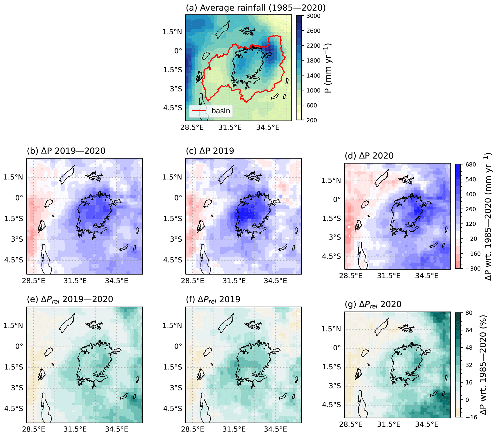
Figure 2(a) Observed average annual precipitation from PERSIANN-CDR for the period 1985–2020. The Lake Victoria basin outline is shown in red. Absolute precipitation anomaly in the years (b) 2019–2020, (c) 2019, and (d) 2020. Relative precipitation anomaly in the years (e) 2019–2020, (f) 2019, and (g) 2020. All anomalies are calculated with respect to the period 1985–2020.
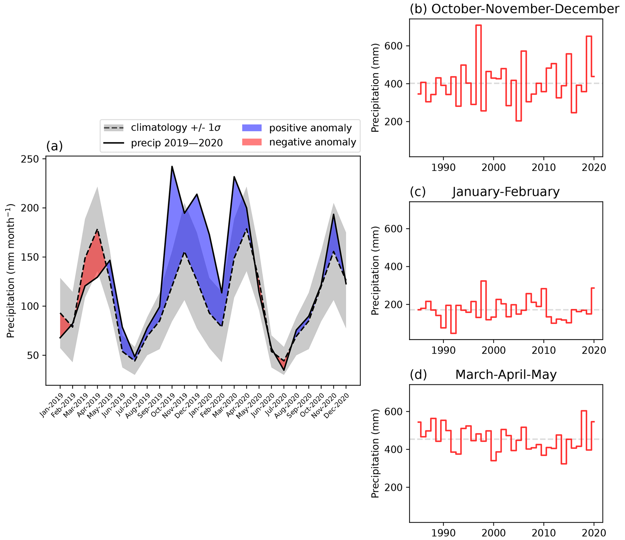
Figure 3(a) Monthly accumulated precipitation over Lake Victoria and its basin for the period 2019–2020, shown relative to the climatology (calculated based on the period 1985–2020). Periods of positive anomaly are shown in blue, and periods of negative anomaly are shown in red. (b) Accumulated precipitation in OND rainy season, JF dry season, and MAM rainy season, with the long-term seasonal average for the period 1985–2020 shown as a dashed grey line.
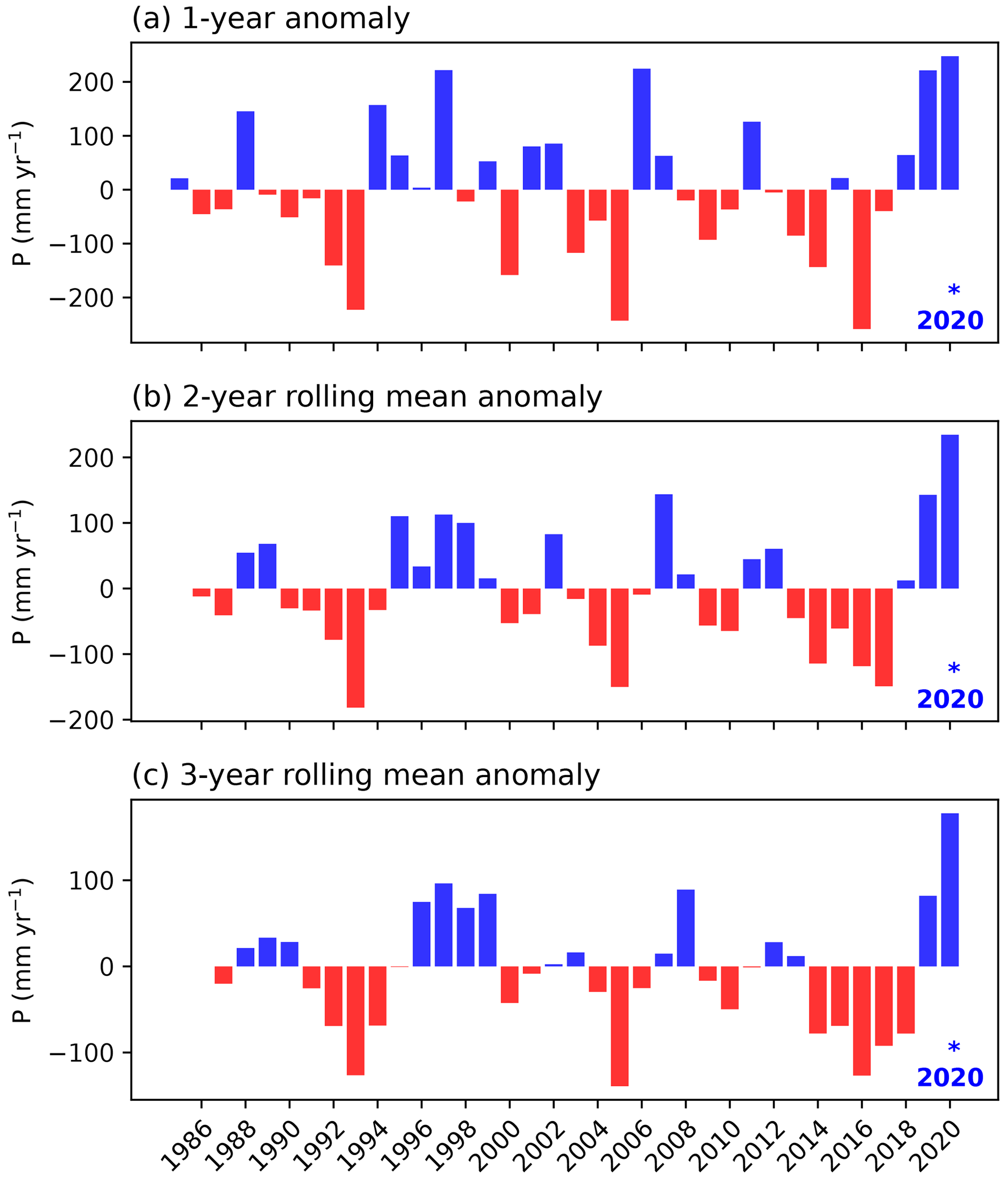
Figure 4Annual accumulated precipitation anomaly with respect to the period 1985–2020 in the Lake Victoria basin for (a) 1 year, (b) a 2-year rolling window, and (c) a 3-year rolling window. The record-breaking year is marked with an asterisk.
3.2 Estimation of flooded area and affected population
Based on remote sensing analysis, a total area of approximately 642.5 km2 in the lake basin within 50 km of the lake shores is estimated to have been affected by flooding between April and July 2020 (Fig. 5). This corresponds to approximately 0.9 % of the 50 km buffer around the lake shores. Key areas identified as flooded include the basins of the Nzoia and Yala rivers and the Kisumu and Homa Bay Counties in Kenya; the floodplains of large rivers (including the Mara, Grumeti, Simiyu and Kagera rivers) in Tanzania; and shoreline and wetland locations near Masaka, Entebbe, and Kampala and along the coasts of lake islands in Uganda. Flooding is also detected along the shoreline of most of the lake. Within 50 km of the shores of Lake Victoria, a total of 29 070 people are estimated to have been affected by flooding between April and June 2020, which corresponds to about 0.12 % of the total population living in this area (23 million people). The affected population is identified throughout the area in both coastal and inland locations near river floodplains.
Detailed visual analysis of SAR images for the Nzoia River basin, which was reported as heavily affected in media, shows important flooding between April and May 2020. The area is mostly non-flooded on 2 April (Appendix Fig. C6a) and starts to show early signs of flooding in late April followed by important flooding on 8 May 2020 (Appendix Fig. C6b, d). By 20 May, large parts of the floods have receded, but some traces are still visible along the floodplain and in the southern and south-eastern sections of the area (Appendix Fig. C6c). Overlaying the area detected as flooded by the HASARD algorithm in the Nzoia basin between April and June 2020 with gridded population data allows us to identify where people were affected by flooding (Fig. 6).
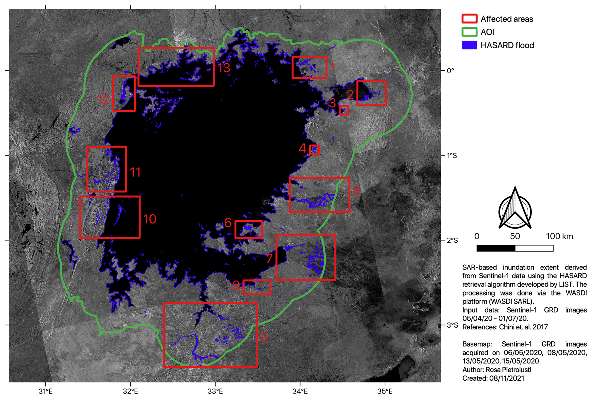
Figure 5Key areas affected by flooding as detected by the HASARD automated flood event retrieval algorithm of LIST (Luxembourg), over the period April–June 2020, limited to an area within 50 km from the lake shoreline (area of interest, AOI): (1) Nzoia and Yala rivers, Busia–Siaya counties, Kenya; (2) Sondu and Nyando rivers, Kisumu–Homa Bay Counties, Kenya; (3) Olare, Homa Bay County, Kenya; (4) River Kuja, Migori County, Kenya; (5) Mara River, Mara Region, Tanzania; (6) Makojo, Mara Region, Tanzania; (7) Grumeti and Mbalangeti rivers, Mara Region, Tanzania; (8) Simiyu River, Simiyu Region, Tanzania; (9) Magongo and Isanga Rivers, Mwanza Region, Tanzania; (10) Muleba district, Kagera region, Tanzania; (11) Bukoba rural district, Kagera region, Tanzania; (12) Masaka area and Ssese Islands, Central Region, Uganda; and (13) Entebbe–Kampala area and islands, Central Region, Uganda.
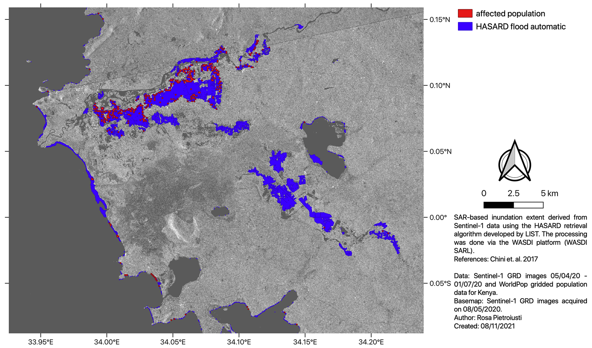
Figure 6Flood-affected populated grid cells (red) in the Nzoia–Yala area (box 1 in Fig. 5), estimated by combining the flooded area between April and June 2020 (blue) retrieved using the HASARD algorithm of LIST (Luxembourg) and population data provided by WorldPop.
Estimates of population affected by flooding in the Lake Victoria area and the larger eastern Africa region vary widely between media, grey literature, disaster response reports, and the disaster database EM-DAT (Table 1). In part this is because they refer to different geographical areas and time periods. The estimate of people affected by flooding over the larger eastern Africa region in 2019–2020 spans from 700 0009 to over 2 million people10. The disaster database EM-DAT reports over 980 000 affected people and 326 casualties including all flooding events in Uganda, Kenya, and Tanzania for the period between April and November 2020. Filtering the EM-DAT entries to include all those that which include parts of the regions included in our study area (outline in Fig. 5) results in over 830 000 affected people and 292 casualties, with the highest number of people affected in Kenya. However, these EM-DAT entries include many administrative units that are far from Lake Victoria and therefore unrelated to our study area (Guha-Sapir et al., 2022, Table 1).
Analysis of media sources covering the studied regions give an estimate of approximately 32 500 to 54 800 affected people aggregated over the three countries, which broadly agrees with our remote-sensing-based estimate (Table 1). For instance, in Kenya, media sources from May 2020 report 3000 people left homeless in the Budalangi constituency of Busia County11 (Fig. 5 box 1). As an effect of the Nzoia River flood in early May 2020 alone, UN OCHA reports at least 40 000 people were made homeless12. Media sources report 400 families still displaced in August 2020 due to the Nzoia floods13. Later in the year, in October 2020, the Kenya Red Cross society reported 7000 homes affected by Lake Victoria backflow in the Budalangi Constituency of Busia County, Kenya14. Other media sources report 3000 people displaced in the Rachuonyuo Sub-county of Homa Bay County due to backflow15 (Fig. 5 boxes 2–3). A conference held by the Aga Khan University with representatives of local governments, the International Federation of the Red Cross and Red Crescent societies, and universities, reported almost 20 000 people displaced in Busia County, 3000 in Siaya County, and 700 in Homa Bay County in Kenya16 (Fig. 5 boxes 1–3). In Uganda, media reports more than 3800 people displaced from the lake islands in the Mayuge district17 18 (Fig. 5 east of box 13), whereas important flooding was not identified using HASARD in these islands. In Tanzania, disaster response sources report approximately 5000 people impacted in the Kagera and Musoma regions19.
Guha-Sapir et al. (2022)Guha-Sapir et al. (2022)Guha-Sapir et al. (2022)Table 1Estimates of the number of people affected by flooding in 2020 in the Lake Victoria basin and larger eastern Africa region, compiled from different sources.
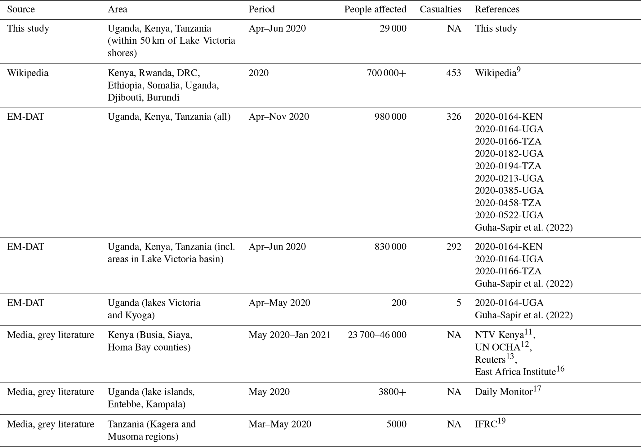
NA: not available.
3.3 Event definition
As outlined in Sect. 1.1, we focus on the rate of change in lake levels () instead of on absolute lake levels to define the event, choosing a time window (Δt) of intermediate length corresponding to 180 d, and subsequently extract annual block maxima of the time series. The 2020 event thus defined corresponds to a lake level increase of 1.21 m that occurred in the 180 d leading up to 17 May 2020, and is the third most extreme event since 1897, ranking after 1998 (1.39 m) and 1962 (1.30 m; Fig. 7). Lake levels usually rise by approximately 0.28 m in the period November–May, meaning the 2020 event approximately represents a 0.93 m anomaly compared to the whole time series. No clear temporal trend is visible in the resulting time series, although a clustering of high values is visible between 1960 and 1962 (Fig. 7b). We test the sensitivity to this choice of event definition in Sect. B3.
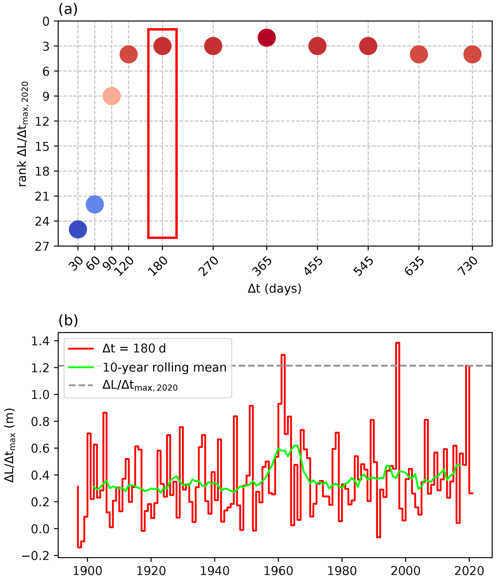
Figure 7(a) Rank of the 2020 event in the 1897–2021 time series of annual block maxima of the rate of change in lake levels () based on the size of the time window (Δt). Red indicates a higher rank (more extreme), while blue indicates a lower rank (less extreme). The rank of the 2020 event with the chosen event definition (Δt=180 d) is highlighted by the red box. (b) Annual block maxima time series ( with Δt=180 d for the period 1897–2021 and 10-year rolling mean of the time series.
3.4 Water balance modelling
3.4.1 Water balance modelling: model evaluation
The water balance model forced with observational data reproduces the observed lake levels reasonably well (Fig. 8). The model generally captures the timing of increasing and decreasing levels, but sometimes underestimates or overestimates the magnitude of these variations resulting in a mean bias of 0.06 m and a root-mean-square error of 0.45 m. The large and consistent overestimation from 2005 to 2015 could be due to the modelled outflow, which was assumed to follow the Agreed Curve from 2005 on (Fig. C3), while in this period, the real outflow likely exceeded the Agreed Curve, resulting in lower lake levels (Vanderkelen et al., 2018a). Nevertheless, the model does not show systematic wet or dry biases, which justifies its use for the attribution analysis. Moreover, as the attribution variable is based on lake level variations, biases in absolute levels are less relevant. The lake level peak in May 2020 is reproduced by the model, but underestimated by 0.41 m (Figs. 8 and C8a). Between May 2018 and January 2020, the model reproduces observational lake levels well, but from then on it consistently underestimates lake levels (Appendix Fig. C8a, b). The divergence between modelled and observed levels is fastest between January and May 2020 (Appendix Fig. C8c).
For the 180 d rate of change in lake levels, the WBM generally reproduces the time series derived from observations (Fig. 9) but tends to attenuate extremes (Fig. 9a, b, e). Accordingly, the distribution of () shows less extreme high and low values compared to observations (Fig. 9d). Furthermore, the modelled seasonality of is slightly shifted in time, leading observations by about 10 d to 1 month (Fig. 9c). In 2020, the maximum 180 d increase in levels is shifted in time in the WBM simulation compared to observations: in the former it is modelled between September 2019 and March 2020 (with a magnitude of 0.94 m), whereas in the latter it was observed between November 2019 and May 2020 (with a magnitude of 1.21 m). Nonetheless, the annual block maxima time series derived from modelled lake levels leads to an estimate of the rank of the 2020 event that is high and similar to observations, with the 2020 event ranking second after 1998 (Appendix Fig. C9).
Given (i) the overall skill of the observation-driven WBM simulation, (ii) the similarity of the rank of the 2020 event in the modelled and observed time series, and (iii) the application of a simple bias correction (Sect. 2.2.3), we conclude that the WBM can be trusted to attribute the 2020 event in combination with observed lake levels.
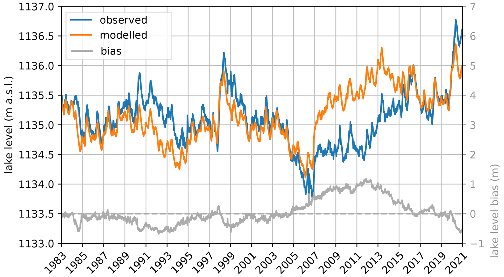
Figure 8Comparison of observed lake levels and lake levels modelled with the observational simulation of the WBM. Model bias is shown in grey (note different scales of the axes).
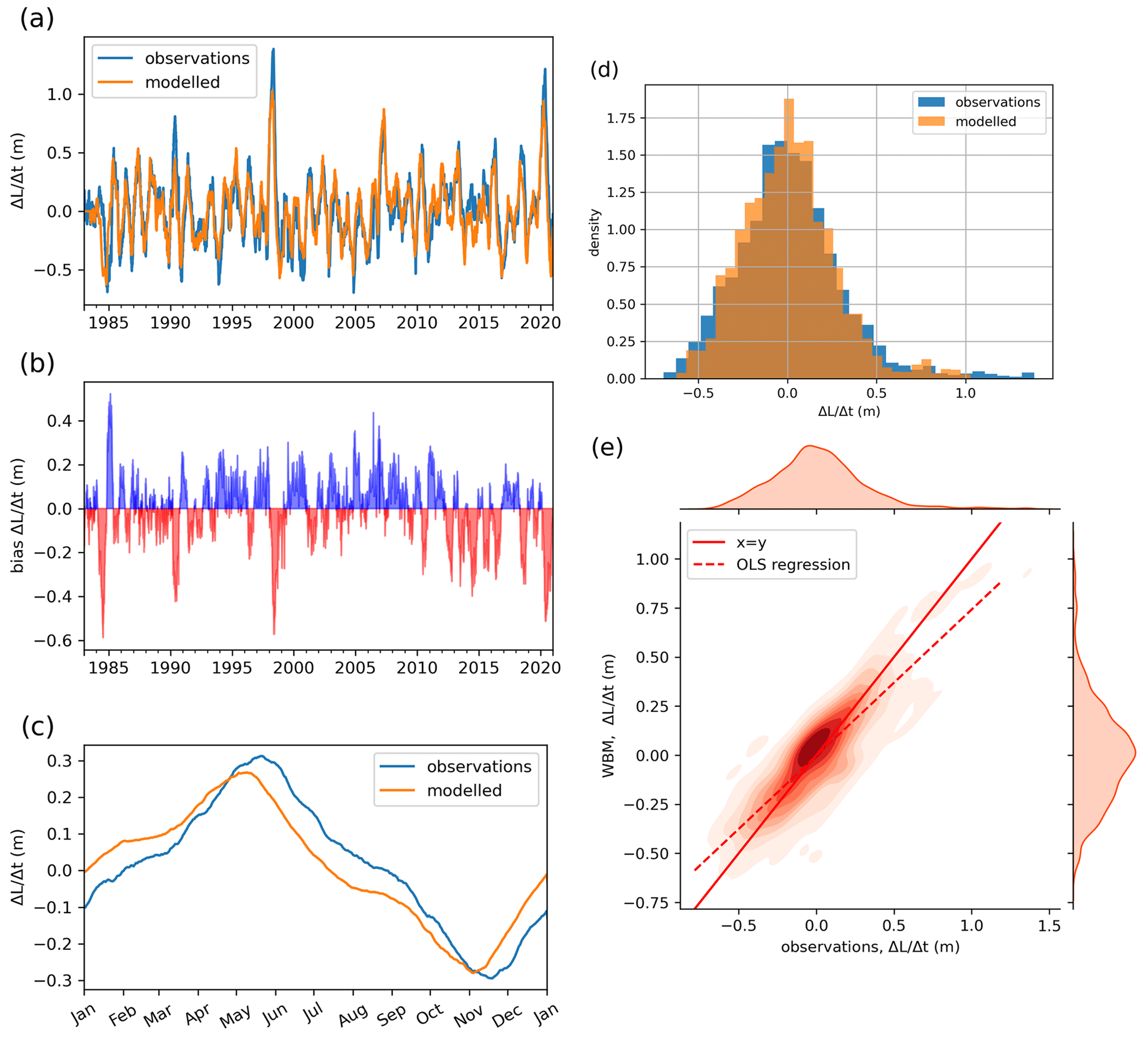
Figure 9Bias in how water balance model represents for Δt=180. (a) Time series of in observations and WBM. (b) Bias in , smoothed with a 3 d rolling window. (c) Climatology of in observations and WBM for overlapping period. (d) Comparing the distribution of the variable in observations and in the WBM. (e) Joint distribution of variable in observations and WBM and ordinary least-squares regression line of best fit through the data.
3.4.2 Water balance modelling: analysis of drivers
The input terms of the lake's water balance reflect the seasonal cycle of precipitation in the basin, with peaks in over-lake precipitation and inflow in the MAM and OND rainy seasons (Fig. 10a). Annually averaged based on the 1983–2020 period, over-lake precipitation supplies 125 mm per month (+75.7 %) and is approximately balanced by an evaporative loss of 123 mm per month (−74.7 %). Inflow provides 40 mm per month (+24.3 %) of input, and 42 mm per month (−25.3 %) is lost through outflow, agreeing with estimates in Vanderkelen et al. (2018a). Lake precipitation has the highest interannual variability (Fig. 10a).
Over-lake precipitation and inflow were generally above average between May 2019 and April 2020 (Fig. 10b–c and Appendix Fig. C10a). Both were particularly anomalous in October 2019 (Fig. 10b), when lake precipitation was a nearly 4 SD anomaly (330 mm) and inflow was a 3.5 SD anomaly (122 mm lake level equivalent) compared to the long-term mean for the month, and they both broke records since 1983.
In the WBM simulation, the maximum 6-month ending in 2020 occurs between September 2019 and March 2020, with a magnitude of 0.93 m. This deviates from observations, where the maximum rise happens between November 2019 and May 2020 and has a magnitude of 1.21 m, which is further discussed in Sect. 3.4.1. Between September 2019 and March 2020, accumulated over-lake precipitation and inflow reached levels similar to their total annual long-term average (Appendix Fig. C10b). Lake precipitation saw an anomaly of +0.59 m (+72 %), inflow of +0.26 m (+93 %), outflow of +0.01 m (+40 %), and lake level equivalents compared to climatological average, resulting in a positive residual of approximately +0.75 m (Appendix Fig. C11). This is smaller than the full magnitude of the modelled event (+0.93 m) because 19 % of the 2020 event corresponds to the climatological average rise in lake levels for the period from September to March (+0.18 m), whereas 81 % of the event (+0.75 m) was due to anomalous precipitation and inflow, which were only partially balanced by above-average outflow following the rise in lake levels. Lake precipitation and inflow contributed 70 % and 30 %, respectively, to the anomalous lake level rise. Since this is similar to the historical proportion between the two input terms in the lake's water balance in climatology (see Sect. 1.2), in relative terms these can be understood to have contributed equally to the anomalous rise, although precipitation was a greater contributor in absolute terms.
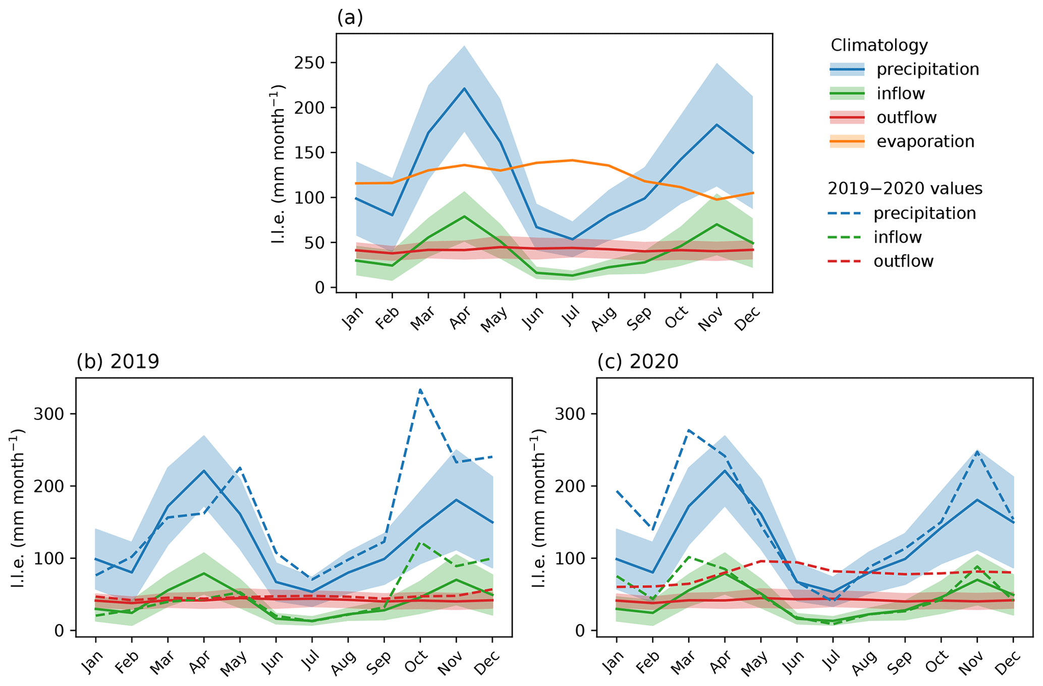
Figure 10(a) Climatology of water balance terms modelled over the period 1983–2020, expressed in lake level equivalent (l.l.e.), with the uncertainty bands spanning 1 standard deviation. Water balance terms in (b) 2019 and (c) 2020 compared to climatology. Evaporation is not shown in (b) and (c) as the annual cycle is fixed by modelling design for all years.
3.5 Observational analysis: return period and trend analysis
The 2020 observed increase of 1.21 m is estimated to have a return period of 63.2 years in the current climate (CI 27–395 years; Fig. 11a–b). This implies that if we have no prior information on circulation, sea surface temperatures, dam management, or further increases in GMST, there is a 1.6 % chance each year of experiencing a 180 d lake level increase of 1.21 m in today's climate. The large confidence interval indicates there is considerable uncertainty in the estimate, meaning this could be quite a common event that we expect to occur every few decades, or it could be quite a rare event, expected to occur only every few hundred years. In a pre-industrial climate, the event has an estimated return period of 104 years (CI 43–1097 years), which results in a probability ratio of 1.7 (CI 0.3–3.9), indicating that the event is estimated to be 1.7 times as likely in the current climate compared to a pre-industrial climate. The confidence interval does however not exclude 1, meaning that uncertainty includes the possibility that no detectable change in the likelihood of the event has occurred. In a pre-industrial climate, lake levels would have risen 0.11 m (0–0.23 m) less than observed, with uncertainty including the possibility of no attributable change. Observational results for key distribution parameters and return periods are shown in Tables 2 and 3. The estimated return period of the event in the current climate is taken as the return period to calculate a model-specific magnitude threshold that represents the flood event in each climate model historical and hist-nat simulation pair.
While some non-homogeneity is introduced in the time series due to a different temporal resolution of lake level observations in 1896–1948 (monthly) and 1948–2021 (daily to 10-daily), we test the sensitivity of the observational attribution to this, by artificially reducing the resolution of the entire lake level time series from daily to monthly and repeating the return period estimates. The results are robust, giving similar estimates of the return period of the event in the current climate (best estimate of 63.5 years, CI 27–426 years), and of the probability ratio (best estimate 1.4, CI 0.2–3.4) and magnitude change (best estimate +7 cm, CI −4 cm to +20 cm) compared to a pre-industrial climate.
Furthermore, we test the sensitivity of our estimates to the presence of overlapping blocks in the annual block maxima time series (see Sect. B3 and Appendix Fig. C7). We exclude the overlapping blocks by removing any year with a block ending between October and December. Results give similar estimates of the return period of the event in the current climate (best estimate of 64.8 years, CI 27–467 years) and of the probability ratio (best estimate 1.4, CI 0.2–3.4) and magnitude change (best estimate +8 cm, CI −4 cm to +23 cm) compared to a pre-industrial climate.
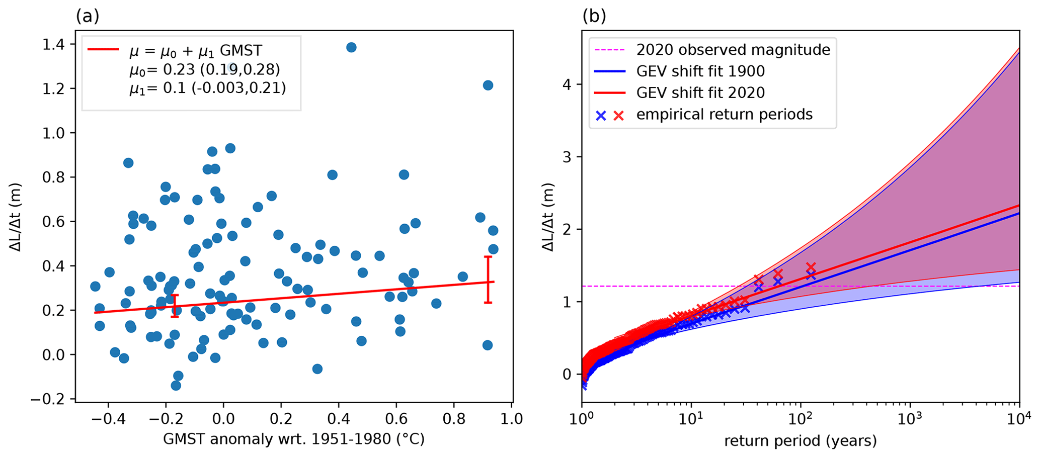
Figure 11GEV shift fit to annual block maxima time series based on observed lake levels for the period 1897–2020. (a) Linear model of the location parameter μ as a function of the GMST covariate based on the estimated parameters μ0 and μ1. The vertical red lines show the best estimate and 95 % confidence interval of the location parameter values in 1900 (pre-industrial climate) and 2020 (current climate). (b) GEV shift fit in current (red) and pre-industrial (blue) climates, based on the shift in the location parameter, with uncertainty intervals calculated by bootstrapping distribution parameters. The year 2020 is included in the fit and is labelled as a horizontal pink line in (b).
3.6 GCM-driven water balance model simulations
3.6.1 GCM evaluation
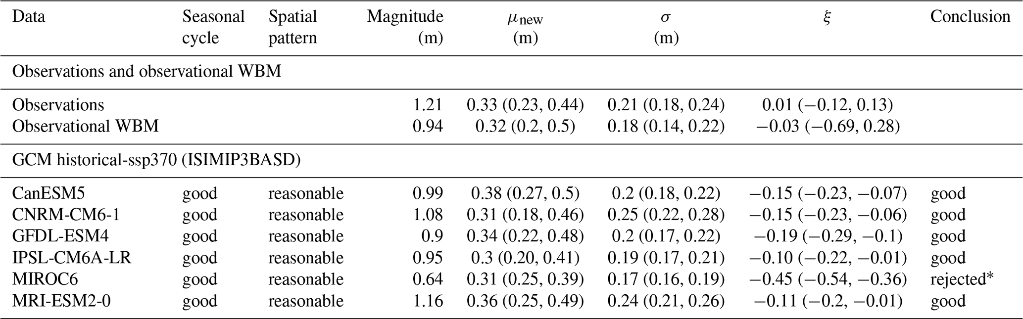
All GCMs, when used to force the WBM, underestimate the magnitude of a 63-year event compared to observations (Table 2). Nonetheless, since the WBM simulations also show this bias when driven by observational precipitation, this could be due to a bias introduced by using the WBM as well as GCM biases in representing precipitation. The location and scale parameters of all distribution fits agree well with each other and with observations (Table 2). While the observational fit results in a slightly positive shape parameter, all GCM-driven fits result in negative shape parameters. Nonetheless, the shape parameter is also slightly negative in the observationally driven WBM simulation, and the confidence intervals of the shape parameters of models and observed lake levels overlap for all models, except for MIROC6, which shows a very negative parameter. For this reason, we reject MIROC6 and exclude this model in further analysis. Both the seasonal cycle of basin precipitation (Appendix Fig. C14) and the spatial pattern (Appendix Figs. C12 and C13) are reasonably represented by all models.
Table 2Validation results based on seasonal cycle, spatial pattern, and fitted scale σ and shape ξ parameters, with 95 % confidence intervals in brackets. Results are shown for observed lake levels for the period 1897–2020 (observations), lake levels simulated by the WBM driven by observational precipitation for the period 1983–2020 (observational WBM), and lake levels simulated by the WBM driven by GCM simulations. For observations and the observational WBM the magnitude of the 2020 event is shown. For GCMs the magnitude of a 63-year event in the current climate estimated based on a non-stationary GEV fit is shown. The location parameter μnew represents the current climate. * MIROC6 is rejected from the analysis due to statistical parameters.
3.6.2 Multi-model attribution
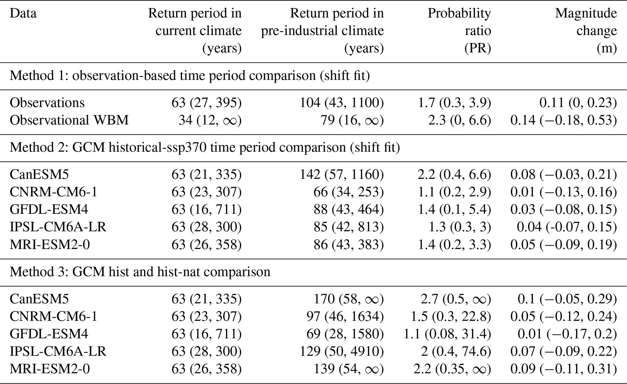
The attribution signal is similar in observed lake levels and historical climate model simulations. Based on WBM simulations driven with historical GCMs and applying a shift fit, a 1-in-63-year event in the current climate is modelled to be slightly rarer in a pre-industrial climate in all models, with best estimates of the pre-industrial return period ranging from 66 to 142 years. This leads to best estimates of probability ratios between the current and pre-industrial climates that are slightly above unity, ranging from 1.1 to 2.2 across historical simulations (Table 3, Method 2). Nonetheless, none of the confidence intervals for the probability ratios exclude unity. Similarly, all GCMs indicate an increase in the magnitude of the event between a pre-industrial and a current climate, with best estimates ranging from approximately 0.01 m to approximately 0.08 m. Nonetheless, the confidence intervals for the change in magnitude of individual models all include zero, suggesting that uncertainty due to natural variability is high.
The non-stationary fits based on counterfactual WBM simulations driven with precipitation from hist-nat (natural forcing only) GCM simulations, show probability ratios near unity and magnitude changes close to 0 (Table A2), indicating that there is no trend in the likelihood of the event due to natural forcings. When combining the historical and hist-nat simulations for each model, the best estimate is that the event has been made more likely and that the magnitude has slightly increased due to anthropogenic climate change (Table 3, Method 3). Nonetheless, all confidence intervals include the possibility of no attributable change, indicating large natural variability. Furthermore, the hist-nat simulations of CanESM5 and MRI-ESM2-0 have infinite upper bounds in the confidence intervals of the return period of the event in a current climate without anthropogenic climate change. This suggests that the event could be extremely unlikely in a counterfactual world but also that the uncertainty of a return period estimate based on these models is very high (Table A2). As a result, the upper bound of the probability ratio estimated combining historical and hist-nat simulations of these two models is also infinity (Table 3, Method 3). To synthesize the results of observations and all models, we cap the upper bound of the confidence interval of the PR from both models to 10 000, assuming anything higher than this to be an overestimation.
Table 3Estimated return periods, probability ratios, and magnitude changes of the flood event in a current and a pre-industrial climate based on observed lake levels for the period 1897–2020 (observations), lake levels simulated by the WBM driven by observational precipitation for the period 1983–2020 (observational WBM), and factual (historical) and counterfactual (hist-nat) climate model simulations. In Methods 1 and 2 “current” corresponds to a 2020 climate, while “pre-industrial” corresponds to a 1900 climate. In Method 3 “current” corresponds to a 2020 climate in historical simulations, while “pre-industrial” corresponds to a 2020 climate in hist-nat simulations. Only models that passed the evaluation are shown.
3.7 Hazard attribution synthesis
Synthesizing observations and models, the best estimate is that the event is approximately 1.8 times as likely in the present-day climate compared to a pre-industrial climate (CI 0.8–15.8, Fig. 12). Models and observations generally agree on a slightly positive best estimate for a PR but with a confidence interval that always includes unity. Further, the intra-model uncertainty due to internal variability is larger than the inter-model uncertainty due to model disagreements. The upper bound of the confidence interval of the probability ratio is determined by the chosen limit to the unbounded confidence intervals of the probability ratios of CanESM5 and MRI-ESM2-0, and it thus should be interpreted with caution. Further, the best estimate is that the magnitude of the event has been slightly increased by climate change and that the in a pre-industrial climate an event with a 63-year return period would have led lake levels to rise by 7 cm less than observed. Nonetheless, the confidence interval ranges from no attributable change in magnitude to a possible 14 cm attributable increase in lake levels, which would correspond to 9350 m3 of water.
Although the best estimates indicate a slight increase in the likelihood and magnitude of the event in the current climate compared to a pre-industrial or counterfactual climate, the confidence intervals of the synthesized PR and magnitude change both include the possibility of a null signal. This indicates that uncertainty due to natural variability is large, and results include the possibility that there is no detectable change in the likelihood or magnitude of the event that is attributable to anthropogenic climate change. Further, the uncertainty estimated through bootstrapping is a measure of natural variability, but neglects epistemic model uncertainty, for example that related to the impact of anthropogenic climate change on atmospheric dynamics, and neglects the uncertainty linked to potential confounding factors that are not included in the statistical modelling applied here. This could point at a potentially larger true uncertainty than quantified here. Nonetheless, for a variable related to seasonal precipitation accumulations, which is less directly associated with the thermodynamical effects of anthropogenic climate change than short-duration precipitation extremes, and with no conditioning on modes of climate variability applied, the general agreement between models is conspicuous and points to a possible, albeit potentially weak, role of anthropogenic climate change in the 2020 flood event.
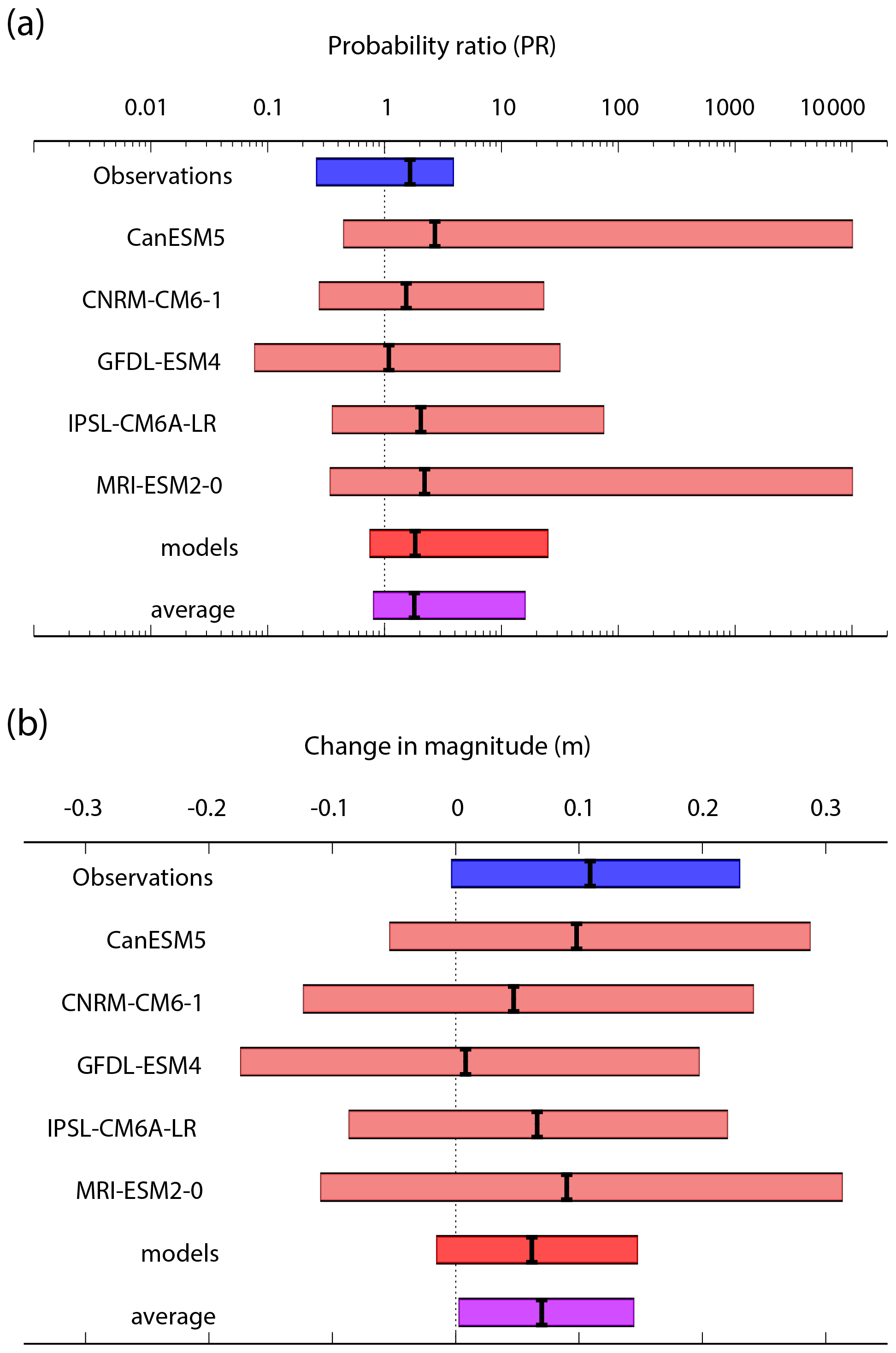
Figure 12Synthesis of (a) PR and (b) change in magnitude estimates from observations and models between a current factual climate and a counterfactual or pre-industrial climate, following the methodology explained in Philip et al. (2020). Coloured bars indicate the 95 % CI, with the best estimate shown as a black line. Uncertainty denotes natural variability and takes model representativity into account but neglects intrinsic epistemic model uncertainty. The red bar is an average of model results, computed through an unweighted synthesis methodology. The purple bar shows the average of observations and models.
The 2020 flooding in the Lake Victoria basin was a high-impact event, which affected tens of thousands of people. Not only the lake shorelines but also tributary rivers flooded. People were impacted both by being displaced and by damage to infrastructure and sources of livelihood. The event occurred while floods and landslides were affecting the wider eastern Africa region, and impacts were compounded by COVID-19 and a locust outbreak that damaged crops (Salih et al., 2020). The event was driven by heavy precipitation that lasted nearly a year and was linked to a positive IOD event, which is known to intensify OND short rains in eastern Africa (Wainwright et al., 2021a). The floods and their impacts were likely also influenced by land use patterns, the type and number of infrastructure and dykes present on rivers, the management of the Lake Victoria dam complex, and people's exposure due to the location of settlements in flood-prone areas. Given this complexity, the attribution carried out here is necessarily a partial study of the event. Nonetheless, it represents a first step towards disentangling the multiple drivers of the event and quantifying the role of anthropogenic climate forcing.
Areas identified as flooded through remote sensing analysis in this study overlap well with areas reported as affected in news and disaster response sources. The flood mapping adds spatial detail to sources that otherwise provide mostly county, district or regional-level information. There are however several ways in which the remote sensing analysis could be refined. First, the HASARD algorithm is known to identify flooding well over farmed and open areas but to perform less well in built-up areas, where trees and partly inundated houses can complicate the backscatter signal Chini et al. (2017, 2019, 2020). Since built-up areas are densely populated, underestimating floods in these areas likely leads to underestimating the number of people affected. Next, much of the identified flood occurred in farmed areas in floodplains, suggesting the floods had an impact on economic activity, which is not taken into account when defining impact only based on resident population affected. Furthermore, the HASARD algorithm overestimates flood over open waterbodies through the detection of waves on the water surface that temporarily increase surface roughness. This spurious flood signal is partly removed by using permanent waterbody masks, but some overestimation of flood could still be present, in particular around the lake shoreline. These sources of error could be estimated by comparing HASARD-derived flood maps with high-resolution optical imagery over a small study area.
The WBM performs well in the observational period, with the water balance of the lake closing without applying a residual term, in the same way as in Vanderkelen et al. (2018a, b). Our WBM simulations show that the rapid rise in lake levels was driven by anomalous precipitation and inflow, accumulated between late 2019 and mid 2020. The modelling setup does not account for various factors, which could be additional drivers. First, land use along rivers that are tributaries of the lake was reported in the media as a compounding factor due to decreased vegetation cover causing increased erosion, sediment transport, and siltation of river channels and higher peak discharge amounts (Mati et al., 2008; Mugo et al., 2020). The WBM uses land cover data prescribed from the Global Land Cover 2000 project (Mayaux et al., 2003) to calculate runoff from precipitation, but as this is not transient, the impact of land use and land cover change on runoff is not accounted for. For instance, we do not include potential changes such as wetland encroachment that could increase runoff into the lake. Second, the modelling setup assumes lake evaporation follows a climatology during the modelled period and thus omits interannual variations in lake evaporation. Third, other possible drivers of the flood extent and its impacts include human dam management, including of infrastructure along tributary rivers, which are not represented in our model, and outflow from the dam complex at Jinja, Uganda, for which data are not fully available for the 2019–2020 period. Finally, impacts are determined by the exposure and vulnerability of settlements and economic activities, with those located close to the lake shores, within wetlands, or in river floodplains more likely to be affected. The extent to which exposure and vulnerability changes drove flood impacts in 2020 is not quantified here.
The underestimation of the lake level rise simulated by the WBM between late 2019 and mid 2020 corresponds to a bias whereby the WBM mutes the magnitude of the most extreme 6-monthly variations in lake levels. For 2020, this bias could be due to (i) an underestimation of true precipitation amounts in the PERSIANN-CDR data product; (ii) uncertainties in the curve number method leading to an underestimation of true inflow; (iii) an overestimation of true evaporation from the lake surface; (iv) an overestimation of true outflow, which could have been below Agreed Curve levels; or (v) variations in other water balance terms (e.g. groundwater) that are not accounted for in the WBM but might lead the WBM to underestimate peaks in . Since observational outflow was used for the period March–May 2020, an overestimation of outflow could participate to the model bias in the first months of 2020 but is unlikely to be the main cause of the 2020 bias.
In terms of the event definition, the 180 d rate of change in lake levels was found to be a good compromise between representativity of the event and limiting the influence of decadal trends compared to raw lake levels, and allowed us to move beyond an attribution of a meteorological variable to the attribution of an impact-relevant variable (Otto, 2016). Nonetheless, the variable relates only indirectly, through backflow effects, to tributary river floods, which caused a large part of the impacts in 2020. Moreover, an increased frequency of high events can be caused by increased interannual variability in seasonal precipitation, which, if not preceded by already high lake levels, would not necessarily represent a high-impact flooding event. Further, lake levels preceding the event would be influenced by evaporation rates, particularly during dry seasons, which do not vary in our study but might change under climate change. Furthermore, as discussed in Sect. B3, the daily variable does not fully meet the theoretical assumptions of extreme value theory, since it is not independent and identically distributed. Moreover, while some annual blocks extracted from the observations were found to be overlapping, our results were found to be robust, and we find a similar attribution signal when the overlapping blocks are excluded from the analysis (Sect. 3.5). Finally, while we cannot readily assume that our annual block maxima time series is in the asymptotic tail of the distribution of maxima, similar objections can be raised to a number of extreme event attribution studies that study slow-onset extremes (e.g. Philip et al., 2018b; Kew et al., 2021), and while these limitations are recognized they do not impede us from providing useful information on these events (see discussions in, e.g. Philip et al., 2020; van Oldenborgh et al., 2021).
Possible sources of non-stationarity not linked to anthropogenic warming must be considered. Decadal variability linked to atmospheric dynamics and modes of climate variability such as the IOD can introduce a non-stationarity that might be unforced and not linked to anthropogenic warming and that can therefore act as a confounding factor in our analysis (Shepherd, 2014, 2016; Philip et al., 2020). Moreover, other factors such as land use changes and dam management can introduce non-stationarity in observations that is not linked to anthropogenic climate forcings. Finally, the different resolution of data before and after 1948 could also introduce non-stationarity, although our attribution results were found to be robust to an artificial reduction in the temporal resolution of the data (see Sect. 3.5).
Strong dynamically induced variability can introduce uncertainty in frequentist probabilistic extreme event attribution statements (Shepherd, 2016, 2021; Faranda et al., 2020). Probabilistic attribution statements are recognized to be strongest when the greatest source of non-stationarity is thermodynamical and when previous knowledge on the physical processes linking the observed change to anthropogenic forcings are high, as is the case, for instance, in relation to short-duration temperature and precipitation extremes (Otto, 2017, 2020). Further, the shift fit method assumes a linear relationship between anthropogenic forcings (often represented by global surface warming) and the response in the modelled distribution of the variable. More complex interactions are likely in our variable, as seasonal precipitation amounts in eastern Africa are mediated by sea surface temperatures in the Indian Ocean and circulation dynamics (Cai et al., 2018; Wainwright et al., 2019). Decadal variability in precipitation amounts is extensively documented in the region and linked to various factors including ENSO and the IOD (Wainwright et al., 2019, 2021a, b; Cai et al., 2018; Marthews et al., 2019; Nicholson, 2014, 2015, 2017, 2018; Rowell et al., 2015; Ummenhofer et al., 2009; Conway et al., 2005; Dunning et al., 2016). The anomalous precipitation in eastern Africa in 2019 was linked to a persistent extreme positive IOD in the same year (Wainwright et al., 2021a; Khaki and Awange, 2021), which was the strongest on record since 1950 (Nicholson et al., 2022). Previous positive IOD conditions were likely linked to the heavy 1961 and 1998 precipitation seasons in the basin (Wainwright et al., 2021a; Nicholson et al., 2022), which emerged as very rare events in our attribution study as well. The statistical methods applied in this study neglect such sources of decadal variability by assuming anthropogenic climate change is the only source of non-stationarity. According to Philip et al. (2020) decadal variability can be a problem for probabilistic attribution when the variability is larger than the signal of anthropogenic climate change. One possible solution would be to condition the return period estimates on the IOD Dipole Mode Index value observed in 2020 by including it as an additional covariate in the shift fit method, as recently done in Kimutai et al. (2023). Conditioning the analysis on a dynamical state moves towards the storyline approach to extreme event attribution (Shepherd, 2021, 2019, 2016; Otto, 2017; Otto et al., 2015). Previous studies have regressed out the influence of modes of climate variability (as in Philip et al., 2018b, to account for the influence of ENSO on precipitation in Ethiopia), but Cai et al. (2014, 2018) suggest that an increase in frequency and intensity of the positive IOD is projected with climate change in the region, meaning that regressing out its influence could remove a pathway of influence of anthropogenic climate change on the regional climate via a dynamical mediator. Nonetheless, there is currently no consensus on the detection and attribution to anthropogenic forcings of an observed increasing trend in the IOD (Gulev et al., 2021), so it is likely premature to assume we are already observing a climate change signal in a positive observed IOD trend.
Additional scientific challenges are recognized in relation to attributing extreme events and their impacts in the Global South, linked to the limited availability of reliable long-term observational and impact data, sometimes flawed representation of climate processes in models, and high natural variability of some of the variables being attributed, making it harder for a trend to emerge as signal from the noise (Otto et al., 2020a, b). For instance, despite a projected increase in average annual precipitation amounts over eastern Africa in most global and regional climate models participating in the Coupled Model Intercomparison Project Phases 5 and 6 (CMIP5 and CMIP6; Rowell et al., 2015; Akurut et al., 2014; Dunning et al., 2018) and the Coordinated Regional Climate Downscaling Experiment (CORDEX; Souverijns et al., 2016; Olaka et al., 2019), a drying trend was observed in eastern Africa between the mid 1980s and 2010, leading to what has been termed the “East African Precipitation Paradox” (Rowell et al., 2015; Souverijns et al., 2016; Wainwright et al., 2019; Palmer et al., 2023) and to investigations of whether this is linked to a misrepresentation of processes driving seasonal precipitation variability in coupled GCMs (e.g. Rowell et al., 2015; Seager et al., 2019). Recent studies have shown climate model projections of increasing average precipitation in the region are mostly driven by representations of longer and heavier October, November, and December “short rains” in the future (Dunning et al., 2018; Cook et al., 2020), while the observed drying has been linked to a shorter duration of the March, April, and May “long rains” season, which has partly reversed since 2010 (Wainwright et al., 2019; Palmer et al., 2023). An improvement to the attribution carried out here would be to include simulations from different modelling setups, for instance with prescribed sea surface temperatures or dynamics, to control for some of these biases (Stone et al., 2019; Cook et al., 2020). Finally, the coarse resolution of GCMs does not allow us to fully represent the mesoscale processes that characterize the Lake Victoria basin, which are linked to the interaction of the atmosphere with the region's complex orography and the lake surface (Thiery et al., 2016, 2017; Van de Walle et al., 2020, 2021), meaning that higher-resolution convective-permitting models could be of added value (Van Lipzig et al., 2023).
In 2020, heavy rainfall caused Lake Victoria's shorelines to flood and its tributary rivers to spill over their banks, displacing thousands of people and threatening lives and livelihoods. Media and government reports linked the heavy precipitation and subsequent floods to anthropogenic climate change. In this study, we mapped the impact of the floods and investigated the influence of anthropogenic climate change on the event by combining probabilistic extreme event attribution methods with a water balance model of the lake.
Based on remote sensing analysis, we estimate that between April and July 2020 an area of 640 km2 close to Lake Victoria flooded, affecting more than 29 000 people. Impacts were caused by lake shoreline and river flooding. For the attribution analysis, we define the 2020 event as the change in lake level over 180 d. In the 180 d leading up to May 2020, Lake Victoria's levels rose by 1.21 m, ranking as the third most extreme event after 1998 and 1962. The event was driven by anomalous lake precipitation and inflow, which contributed to 70 % and 30 % of the anomalous lake level rise, respectively. Outflow was also above average, but was insufficient to balance the increased input into the lake.
Based on observational data, the flood event has an estimated return period of 63 years (CI 27–395 years) in the current climate, and in a pre-industrial climate lake levels would have risen 11 cm (0–23 cm) less than observed. This change in magnitude is, however, associated with a relatively large uncertainty, including the possibility of no forced change. The WBM forced with observational data reproduces the observed event reasonably well, although it underestimates its magnitude and anticipating its timing. Five out of six climate models reproduce lake level variations well, performing in a similar way to the observational WBM, whereas one model is rejected due to excessive biases. Based on a synthesis of observations and climate model simulations, the observed event is slightly more likely in the current climate than in a pre-industrial climate by a factor of 1.8 (CI 0.8–15.8), although uncertainty is relatively large and includes the possibility of no change. Similarly, we estimate that in the absence of anthropogenic climate change a 63-year event would have resulted in lake levels rising 7 cm (CI 0–14 cm) less than observed, which corresponds to approximately 6 % (0 %–13 %) of the total November–May rise in lake levels.
The multi-model attribution carried out showed agreement in the sign and magnitude of change over all GCMs that passed the model evaluation step, which in turn agreed with observations. For a precipitation-related variable, where attribution statements are generally weaker than temperature-related variables, this is a conspicuous result. Accordingly, natural variability was found to be a greater determinant of uncertainty than inter-model disagreement. Further, while the ensemble of climate models used is small, the choice of using a bias-adjusted ensemble was confirmed by the good spatial and seasonal pattern the models showed and the relatively realistic lake level simulation results. The best estimates for the probability ratios and magnitude changes estimated by models and observations all point to a slight increase in the likelihood and magnitude of the event linked to anthropogenic forcings. Using a larger model ensemble and different statistical methods could strengthen the attribution statement, but irreducible uncertainty linked to high natural variability in the region must be recognized.
While limitations in the models, data, and statistical methods used must be taken into account when interpreting our results, this study provides a first step towards disentangling natural variability from a forced response due to anthropogenic climate change behind the high-impact 2020 Lake Victoria floods. The eastern Africa region is comparatively under-studied in attribution, and high natural variability means that both droughts and floods are common in the region. However, given the high vulnerability of local communities in the region, it is of key importance to better understand how anthropogenic climate change is affecting extreme events in eastern Africa.
A1 Climate model experiments
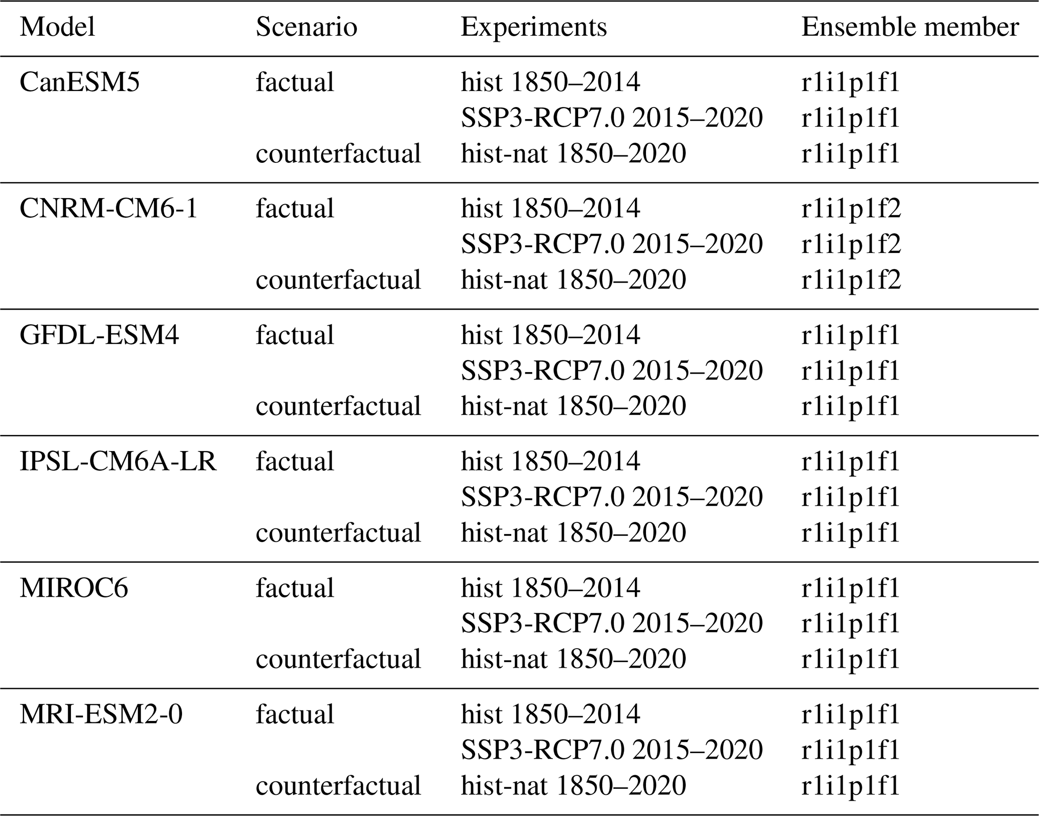
A2 Return period estimates for hist-nat simulations
Table A2Estimated return periods, probability ratios, and magnitude changes of the flood event in a 2020 and a 1900 climate based on counterfactual (hist-nat) climate model simulations using a non-stationary GEV fit. Magnitude changes indicate the difference in lake level rise expected during an event with the same return period. For historical simulations the return period in the 2020 climate is held equal to that estimated from observations to estimate a model-specific magnitude threshold. For hist-nat simulations the model-specific magnitude threshold from the corresponding historical simulation is used to estimate the return periods. Only models that passed the evaluation are shown.
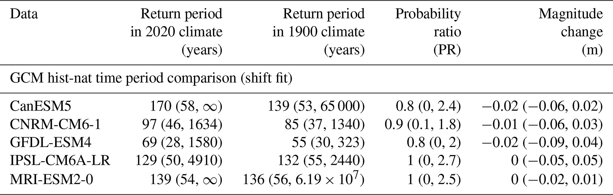
B1 PERSIANN-CDR missing data and comparison with other observational data sources
To assess the importance of the missing days in PERSIANN-CDR data we (i) count the number of missing days per year and per month and (ii) compare the yearly accumulation of precipitation in the Lake Victoria basin with estimates coming from two other state-of-the-art observational datasets: Climate Hazards Group InfraRed Precipitation with Station data (CHIRPS; Funk et al., 2015), obtained for the period 1981–2020, and Multi-Source Weighted-Ensemble Precipitation V2.2 (MSWEP; Beck et al., 2019), obtained for the period 1979–2016. All datasets are remapped to our study area using the same procedure.
PERSIANN-CDR data have 419 missing days, which are concentrated in the early decades of the dataset (Appendix Fig. C2a, b, d). The year with the most missing days is 1984, where a third of all days are missing. Nonetheless, even in the early years, PERSIANN-CDR shows similar accumulated yearly precipitation estimates compared to CHIRPS and MSWEP (Appendix Fig. C2c). Moreover, PERSIANN-CDR generally provides higher estimates of precipitation compared to the other datasets. Correcting for the missing days in PERSIANN-CDR by interpolating between missing values or replacing missing days with their climatological average causes the water balance model to drift and overestimate lake levels, suggesting this correction overestimates true precipitation amounts. For this reason we do not correct for the missing days. We run the water balance model for the whole 1983–2020 period, as this gives very similar results to running the model from 1985. We instead analyse the precipitation anomaly starting from 1985 to avoid overestimating the positive temporal trend in yearly precipitation amounts.
B2 Water balance modelling: curve number method
In the water balance model, the inflow term (Qin) is calculated using the USDA Natural Resources Conservation Service curve number (CN) method to estimate runoff (USDA-SCS, 2004), as in Vanderkelen et al. (2018a). The reader is referred to Vanderkelen (2016) and Vanderkelen et al. (2018a) for more details. The CN method relates accumulated precipitation to runoff based on an empirical relationship. Total runoff is modelled as a function of accumulated rainfall and a parameter referred to as the curve number, which is specific to each land grid cell. The CN parameter is in the range 1 ≤ CN ≤ 100 and is a function of the hydrologic soil type, land use, hydrologic surface condition, and antecedent moisture conditions. The CN method can be summarized by the following equations (Descheemaeker et al., 2008; USDA-SCS, 2004):
where Q is the total runoff (mm) produced by the total accumulated precipitation P (mm); Ia is the initial abstraction parameter (mm), indicating the minimum initial amount of water that must be in the soil before runoff can start; and S is the maximum water retention capacity of the soil (mm), which indicates the maximum amount of water the soil can hold. λ is a dimensionless parameter, commonly set equal to 0.2, which expresses the initial abstraction amount necessary as a fraction of the total maximum soil water retention capacity. As visible in Eq. (B3), S depends on the CN parameter of the soil. The magnitude of the CN determines the proportion of grid cell precipitation that is converted to runoff. The higher the CN, the greater the proportion of precipitation that turns into runoff (Eq. B1). For open waterbodies the CN is set to 100, meaning that all precipitation becomes runoff.
In Vanderkelen et al. (2018a) a CN was assigned to each grid cell in the study area under standard moisture conditions as a function of land cover and the hydrologic soil group (HSG) of the grid cell. Within the water balance model, the CN then varies temporally based on the antecedent moisture condition (AMC), whereby cumulative 5 d antecedent precipitation over the grid cell is calculated, and if this value is below a dry threshold or above a wet threshold (Table B1), the CN of the grid cell is modified based on Eqs. (B4) and (B5).
Each grid cell therefore has three possible CNs. The CN is decreased under dry conditions (CNI<CNII), meaning that maximum soil water retention increases and the proportion of precipitation that becomes runoff decreases. Under wet conditions the opposite is true, the CN is increased by applying the AMC (CNIII>CNII), meaning that the proportion of precipitation that becomes runoff increases. To calculate the inflow term (Qin in Eq. 2), the direct runoff calculated in all basin grid cells is summed for each day. This calculation disregards groundwater flow and any river routing, assuming that all direct runoff calculated in each grid cell immediately enters the lake. Regardless of these assumptions, the model was shown to work well for the Lake Victoria catchment in Vanderkelen et al. (2018a).
Table B1Antecedent moisture condition (based on Vanderkelen et al., 2018a; Descheemaeker et al., 2008).
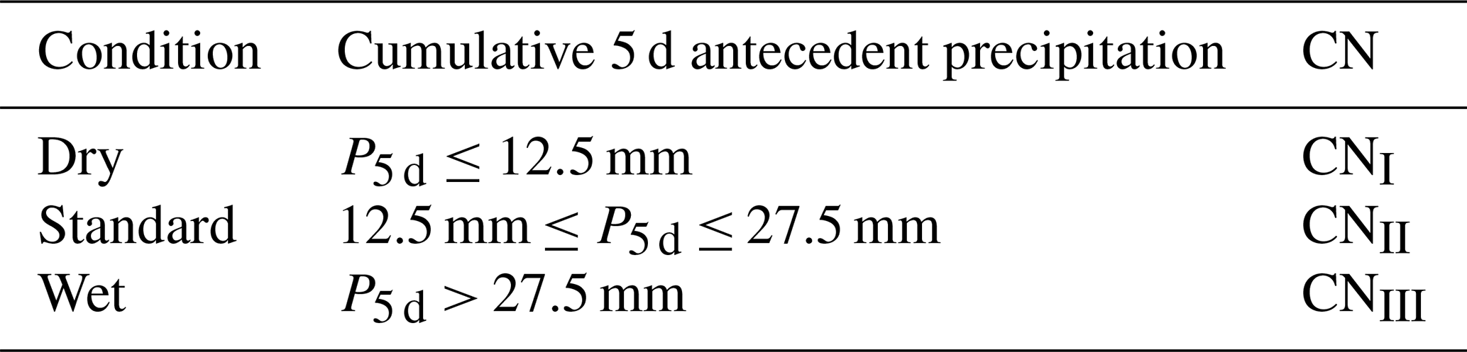
B3 Event definition: sensitivity analysis
We develop a univariate class-based definition of the 2020 flood event. The choice of definition has, on the one hand, to be representative of the event, for example by maximizing its hydro-meteorological extremity or by being as close as possible to its impacts (Philip et al., 2020), but it should, on the other hand, minimize serial correlation and unforced low-frequency interannual trends that violate the statistical assumptions made in the attribution methodology.
As outlined in Sect. 1.1, we focus on the rate of change in lake levels () instead of on absolute lake levels to define the event, reducing the influence of decadal trends. Consequently, an appropriate length of the time window (Δt) has to be selected. A smaller window results in a daily time series that shows less serial correlation, while a larger window reduces the independence of subsequent observations and causes interannual trends to become visible in the daily time series. At the same time, the rate of increase in lake levels observed in 2020 is most extreme when the window is large. When the time window considered is 1 year, the 2020 event ranks second after 1962 (Fig. 7a), while the extremity of the event decreases quickly as the window shrinks to 60 or 30 d (Fig. 7a). An intermediate time window is therefore chosen of 180 d, and the annual block maxima of the time series is extracted. The 2020 event thus defined corresponds to a lake level increase of 1.21 m that occurred in the 180 d leading up to 17 May 2020, and is the third most extreme event since 1897, ranking after 1998 (1.39 m) and 1962 (1.30 m; Fig. 7a, b). Moreover, with this chosen interval, the different temporal resolution of observed lake levels before and after 1948 plays a small role and does not importantly affect return period estimates (see Sect. 3.5).
The 180 d window of each block can extend from the previous year into the calendar year to which the value is assigned. Most of the intervals in the block maxima time series occur in the 6 months between November or December and May or June, capturing lake level increases due to part of the OND short rains season and most of the MAM long rains season (Appendix Fig. C7). There are overlaps only in eight pairs of blocks in the 125-year time series. In these instances, a late time window of the previous year partially overlaps with an early time window of the subsequent year, generally for a 2 to 3 month period. Since this violates the assumption of independence of the annual block maxima time series, we test the sensitivity of our results to these overlapping blocks in Sect. 3.5 and find a similar attribution signal regardless of whether overlapping blocks are included or excluded from the analysis.
Finally, we note that the parent daily variable from which the annual block maxima time series is extracted does not fully meet the theoretical assumptions of extreme value theory (Coles, 2001). These assumptions are that (i) the daily variable is independent and identically distributed, except for the non-stationarity modelled by the shift fit, and (ii) the size of the sample from which each annual block maximum is drawn is sufficiently large such that the distribution of the maxima approaches its limit distribution (here, a GEV). In relation to the first assumption, the realizations of the variable cannot be considered independent since (i) the time window upon which each subsequent daily observation is calculated overlaps with the previous observation for 179 out of 180 d, and (ii) heavy precipitation days are likely to be clustered in time. In relation to the second assumption, we cannot readily assume that we are in the asymptotic tail of the distribution of maxima. Although block maxima are often drawn from a year of daily observations (Hammerling et al., 2019; Coles, 2001), in our case we do not have 365 independent daily observations, but we instead have 365 rolling 180 d windows, meaning that only two windows each year are fully non-overlapping. Further, variability in 6-month rates of change in lake levels depends on relatively low-frequency variability in seasonal precipitation. The block maxima usually detect a part of the signal from the OND short rains season and the whole of the MAM long rains season, resulting in a time window that ends around the month of May in most years. This suggests that we are not extracting each block maxima from a very large sample of independent observations but are instead analysing a time series that is closely linked to seasonal precipitation amounts. Nonetheless, similar objections can be made to a number of extreme event attribution studies that study relatively “slow” climate variables, such as multi-month droughts (e.g. Philip et al., 2018b; Kew et al., 2021), and these limitations are recognized by the community but do not impede the possibility of carrying out such studies and providing useful information (Philip et al., 2020; van Oldenborgh et al., 2020).
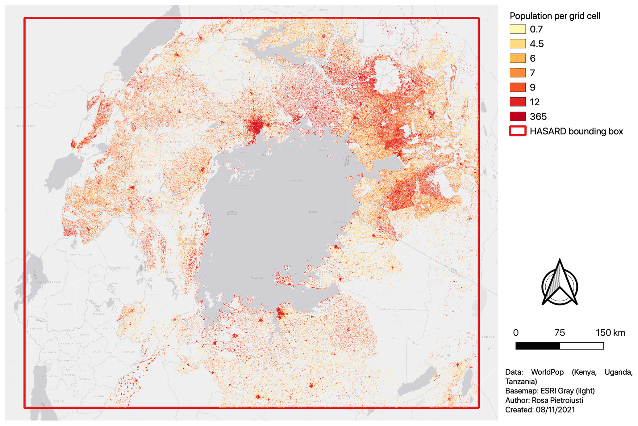
Figure C1WorldPop gridded population data (density per 100 m grid cell) in Kenya, Uganda, and Tanzania, cropped to the study area.
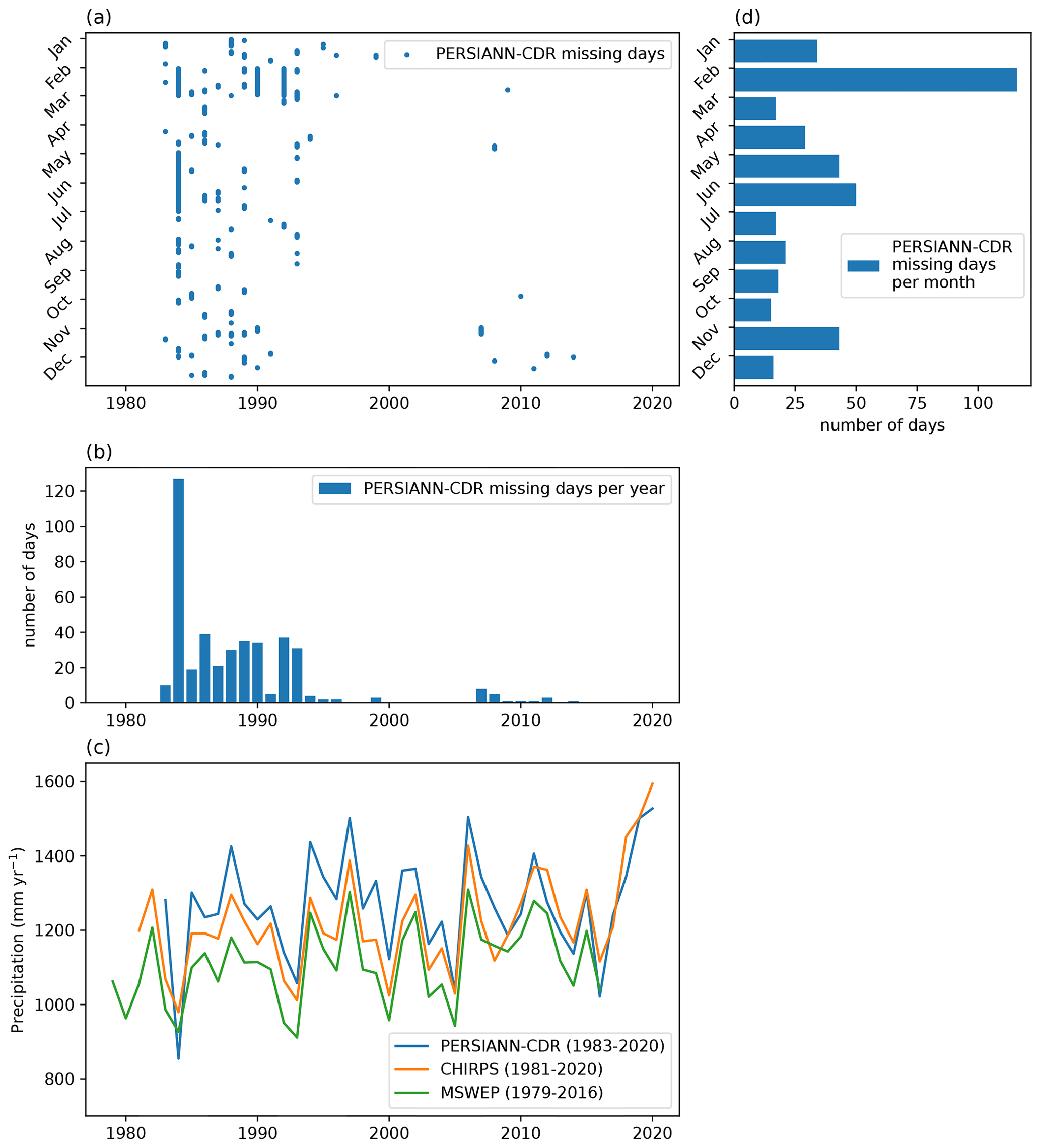
Figure C2Assessment of missing days in PERSIANN-CDR data and comparison with other observational data sources: (a) distribution of the missing days in PERSIANN-CDR each year (419 total missing days in the period 1983–2014), (b) total number of missing days each year, (c) total number of missing days grouped per month, and (d) comparison of yearly accumulated precipitation amounts in the Lake Victoria basin in PERSIANN-CDR, CHIRPS and MSWEP V2.2 (CHIRPS and MSWEP have no missing data in this period).
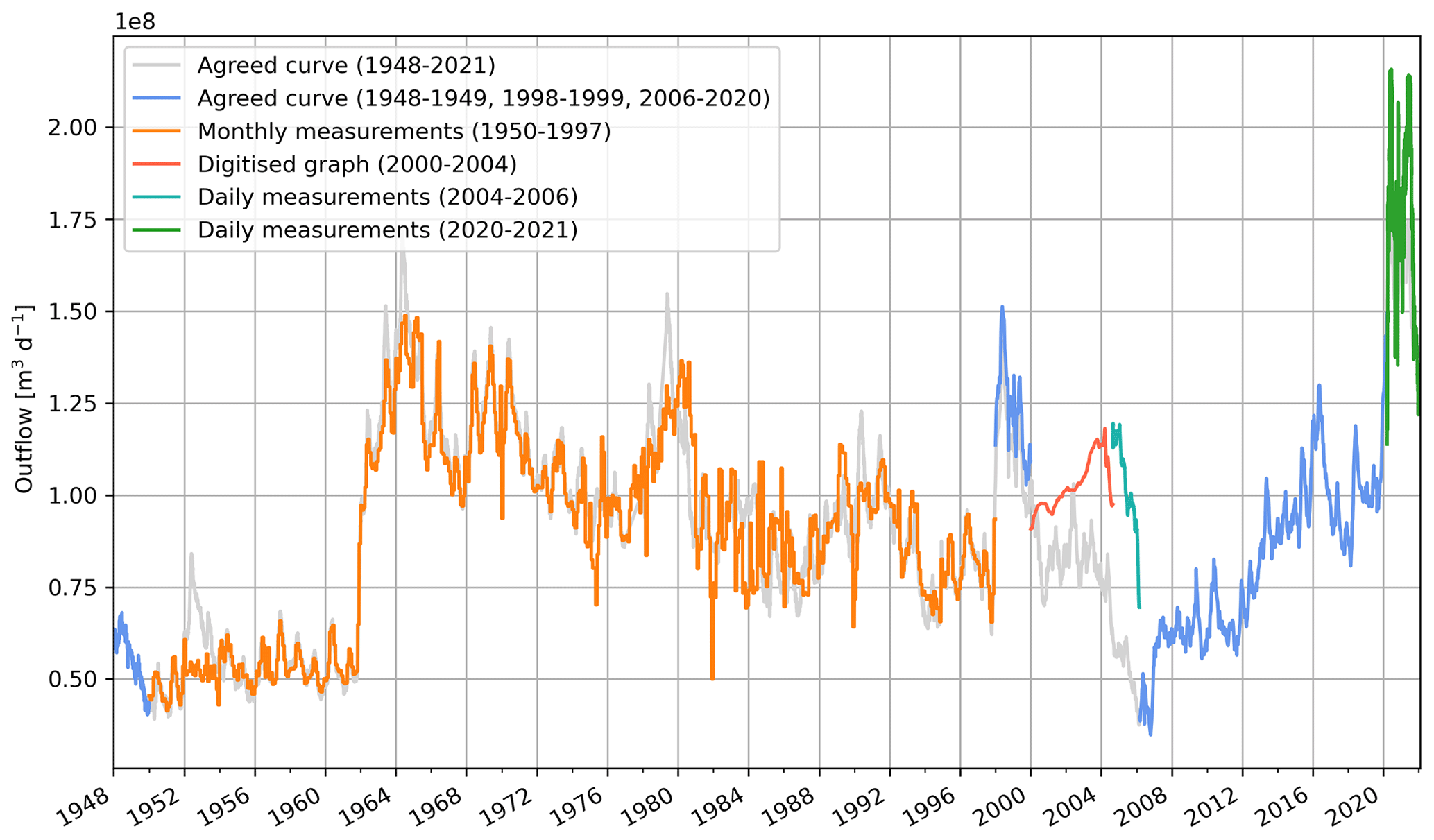
Figure C3Daily outflow time series for the period 1948–2021 compiled from different sources and compared with the Agreed Curve based on observational lake levels. The semi-observational outflow time series is created by extending the composite time series used in Vanderkelen et al. (2018a). For the period 1948–1950, outflow is calculated with the Agreed Curve. From 1950 to 5 March 2006, the outflow time series from Vanderkelen et al. (2018a) is used. In the period 1950–1997 this is based on monthly in situ measurements, for 1998–1999 outflow is calculated with the Agreed Curve, for 2000–2004 outflow is digitized from a graph in Lake Victoria Basin Commission (2006), and from 2004 to 5 March 2006 daily measurements are used. For the period 5 March 2006–17 March 2020 outflow is calculated using the Agreed Curve. From 18 March 2020 to 2021 daily outflow measurements at Jinja are available.
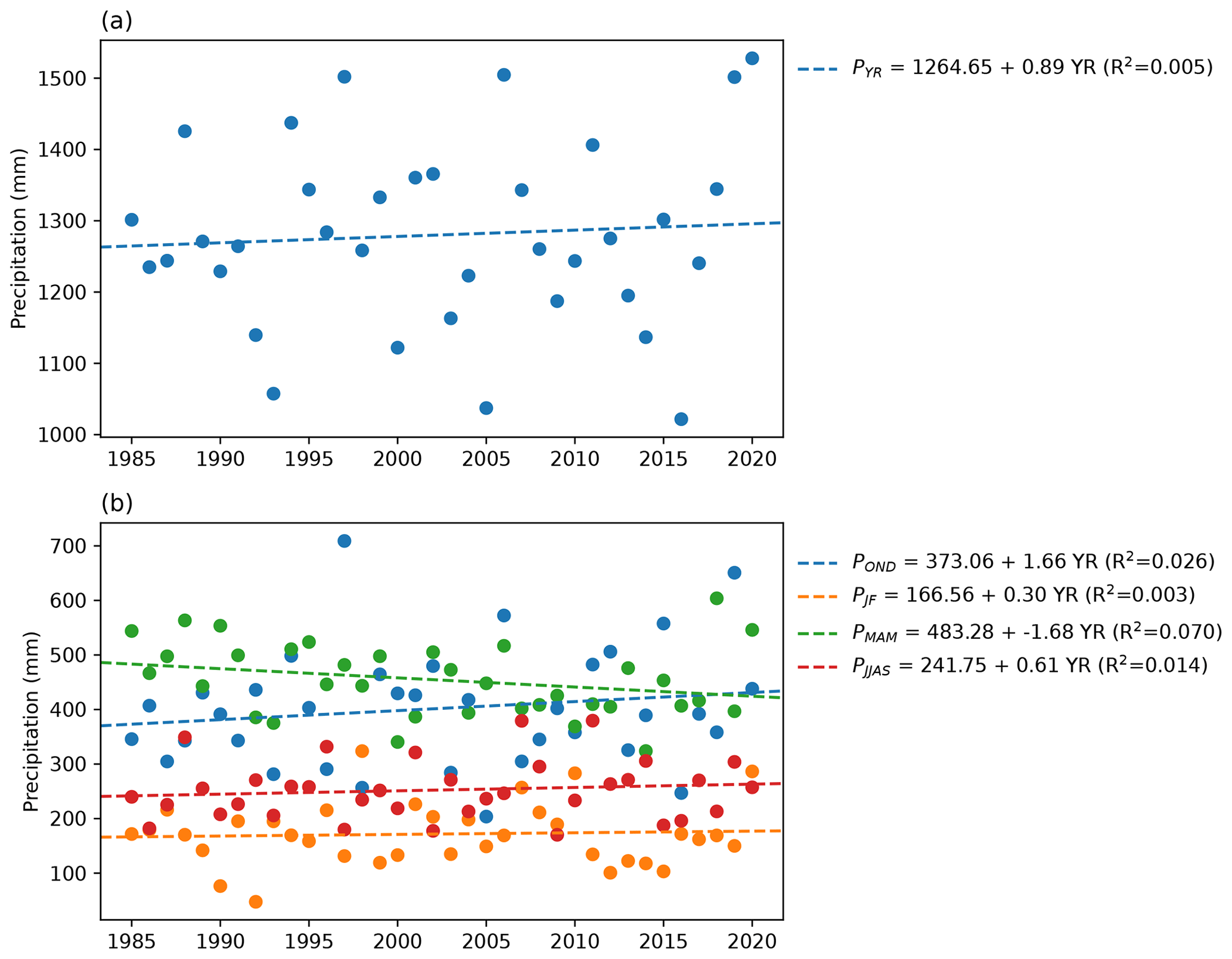
Figure C4Linear regression of (a) yearly accumulated precipitation and (b) seasonal precipitation accumulations in the Lake Victoria basin against time to estimate temporal trend for the period 1985–2020 (values are given in units of mm).
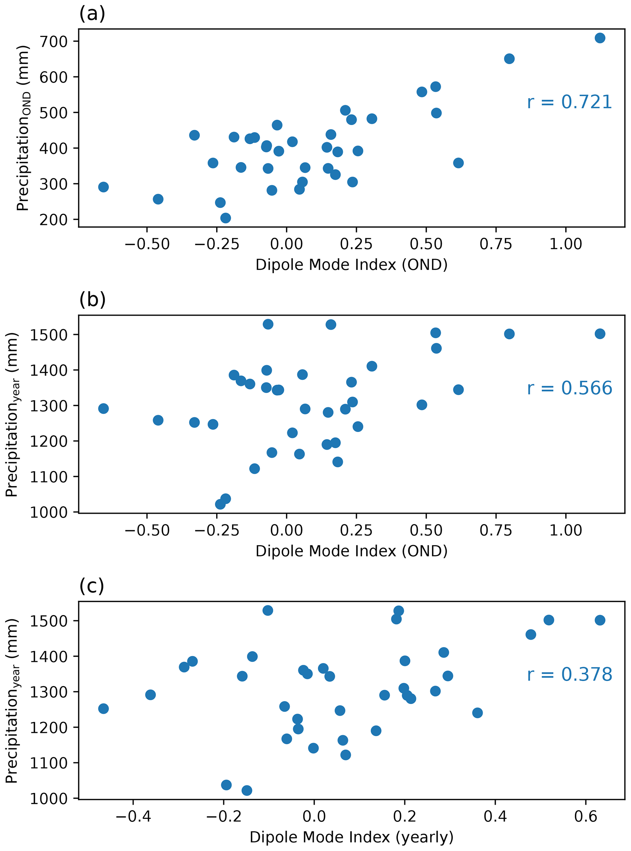
Figure C5Correlation of precipitation in the Lake Victoria basin in the period 1985–2020 with the Indian Ocean Dipole Mode Index. Pearson correlation coefficients are shown for precipitation accumulated during (a) the OND short rains and (b), (c) the whole year, against the Indian Ocean Dipole Mode Index averaged (a), (b) in the months October–December, and (c) across the entire calendar year.
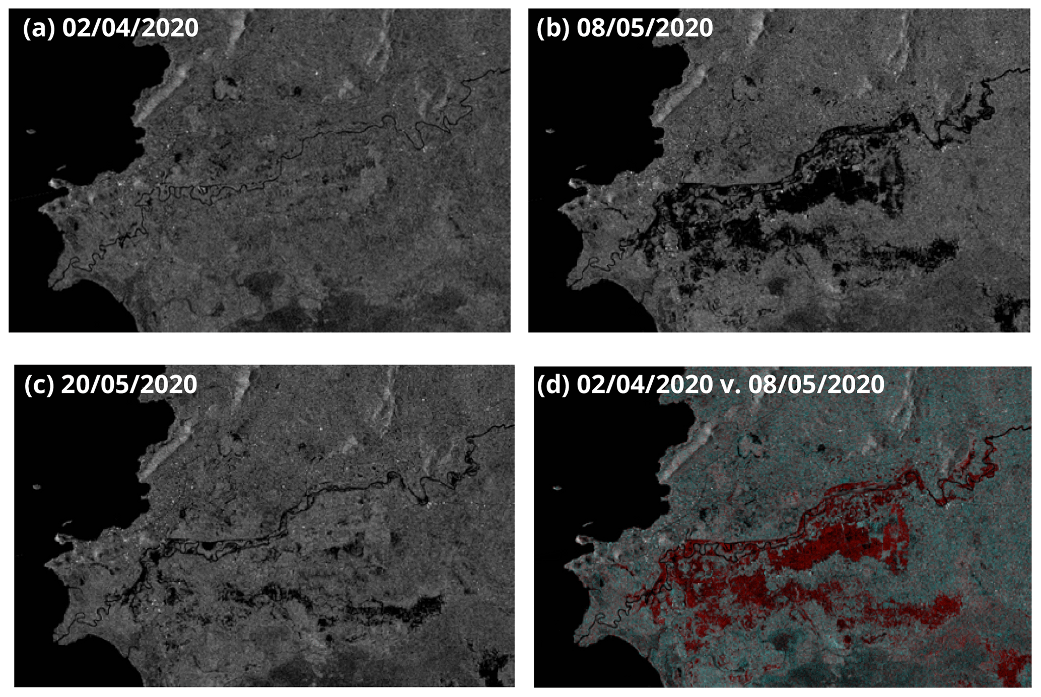
Figure C6Flooding along the Nzoia River from Sentinel-1A SAR GRD images, acquired (a) 2 April 2020 at 16:04:36 and 16:05:01, (b) 8 May 2020 at 16:04:37 and 16:05:02, (c) 20 May 2020 at 16:04:38 and 16:05:03. Darker colours indicate less backscatter due to water. (d) False-colour composite combination of panels (a) (R channel) and (b) (G, B channels), where the flood signal appears in red due to decrease in backscatter between (a) and (b).
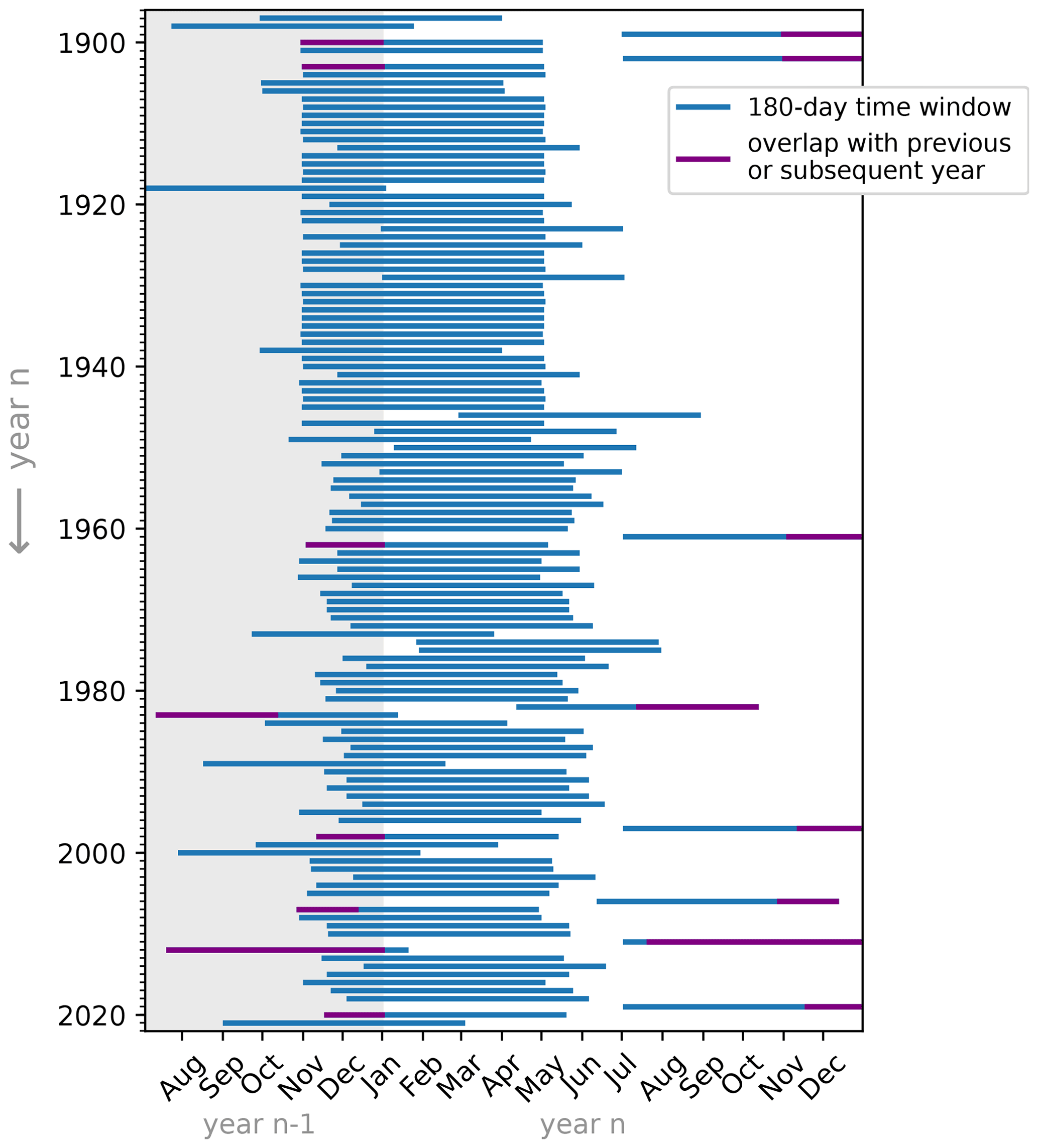
Figure C7The 180 d time windows selected from the time series by the annual block maxima methodology for each year in the period 1897–2021. These indicate the period in which the largest 180 d rate of change in lake levels occurs in each calendar year. The value is assigned to the year in which the final day in the 180 d period is located (year n), but the period can start in the previous calendar year (year n−1). Blue bars do not overlap with blocks of other calendar years; purple portions of the bars indicate a partial overlap with the block of the previous or subsequent calendar year. There are overlaps in the years 1899–1900, 1902–1903, 1961–1962, 1982–1983, 1997–1998, 2006–2007, 2011–2012, 2019–2020. The difference in the temporal resolution of lake level measurements before 1948 (monthly) and after this year (daily to 10 daily) is visible as an increase in variability of the blocks.
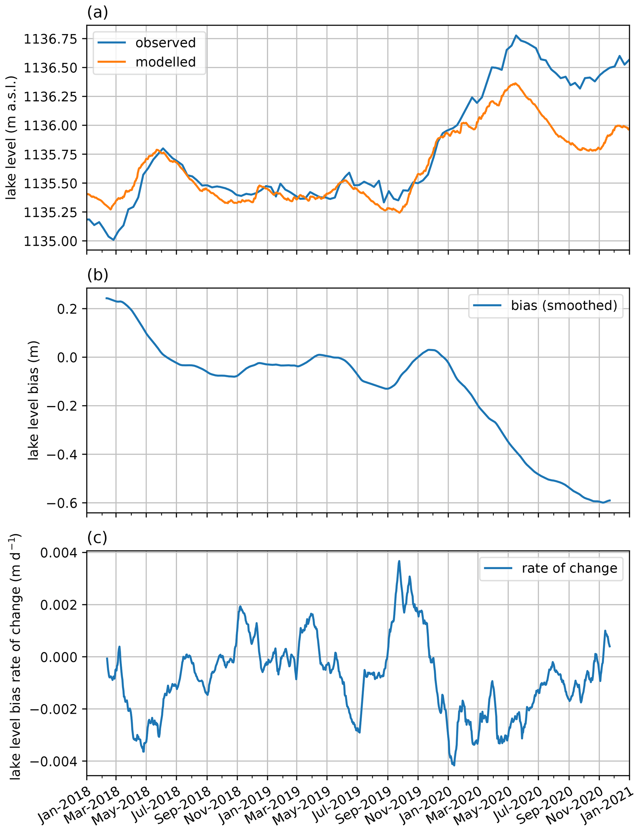
Figure C8Water balance model bias in the period January 2018–December 2021: (a) observed and modelled lake levels, (b) lake level bias (i.e. difference in modelled minus observed curves in a) smoothed with a centred 60 d moving average low-pass filter, and (c) daily rate of change in smoothed lake level bias (i.e. approximation of first derivative of bias curve from b).
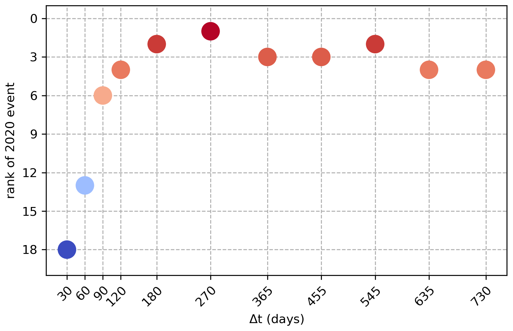
Figure C9Rank of the 2020 event defined as a rate of change in lake levels () based on the size of the time window, from the observational WBM simulation for the period 1983–2020. Red indicates a higher rank (more extreme), while blue indicates a lower rank (less extreme).
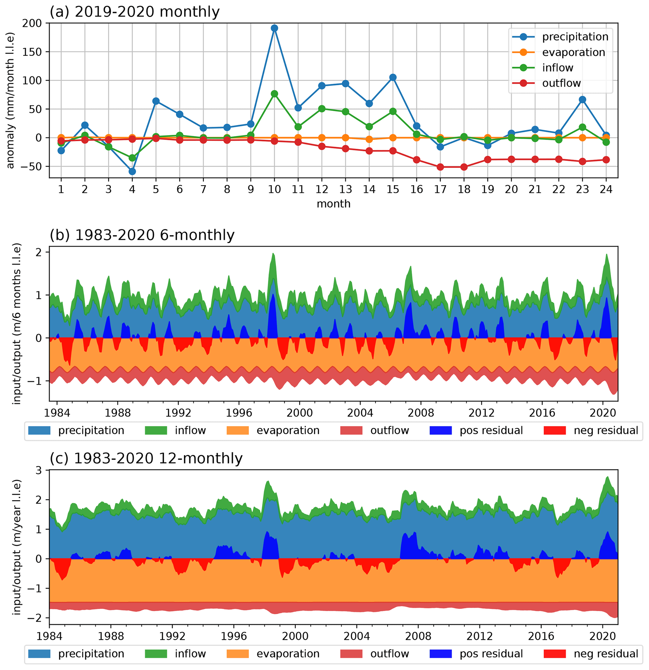
Figure C10(a) Monthly anomaly in each water balance term from January 2019 to December 2020. (b) The 6-monthly accumulated water balance terms (1984–2020) in metres of lake level equivalent and resultant residual in the water balance. (c) Yearly accumulated water balance terms (1984-2020). Accumulated terms are calculated with a rolling window applied to a monthly time series to obtain the cumulative sum over the previous (b) 6 months or (c) year. The residual is the difference between positive terms (precipitation and inflow) and negative terms (evaporation and outflow).
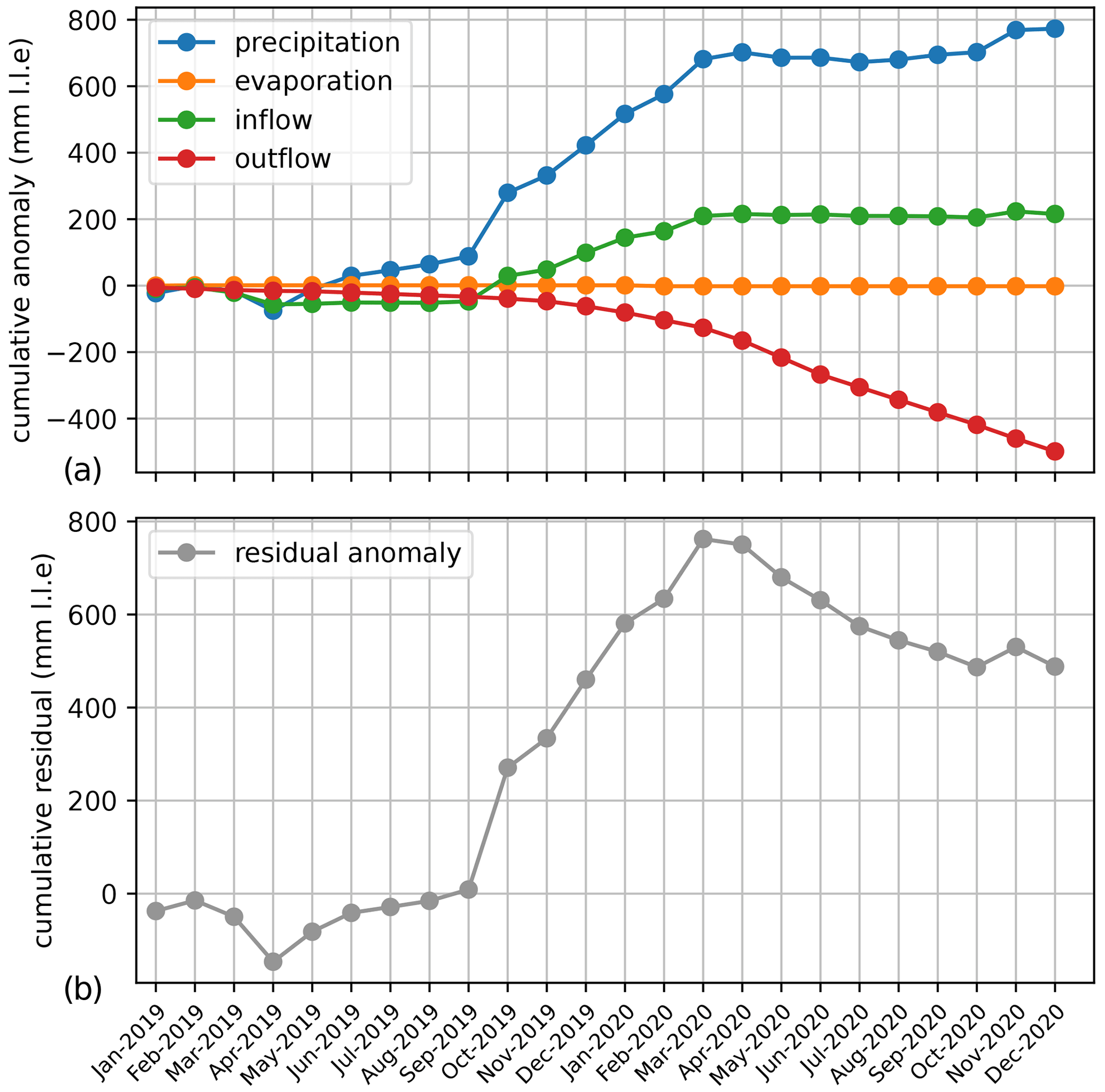
Figure C11Cumulative monthly anomalies in water balance terms from January 2019 to December 2020 (a, cumulative version of Fig. C10a) and resultant cumulative anomaly in the water balance residual term (b).
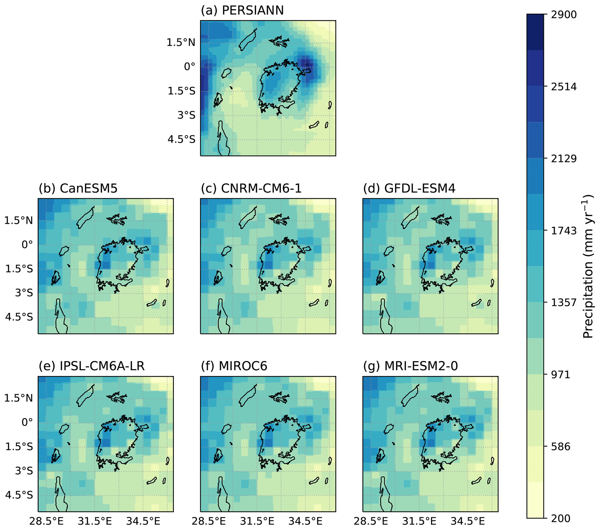
Figure C12Spatial pattern of mean annual precipitation accumulation in Lake Victoria basin in PERSIANN-CDR (a) and GCM historical and SSP3-RCP7.0 simulations (b–g) for the period 1985–2020.
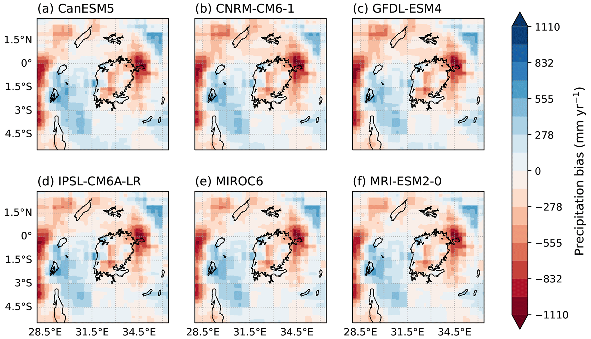
Figure C13Bias in mean annual precipitation representation GCM historical and SSP3-RCP7.0 simulations compared to PERSIANN-CDR observational data for the period 1985–2020.
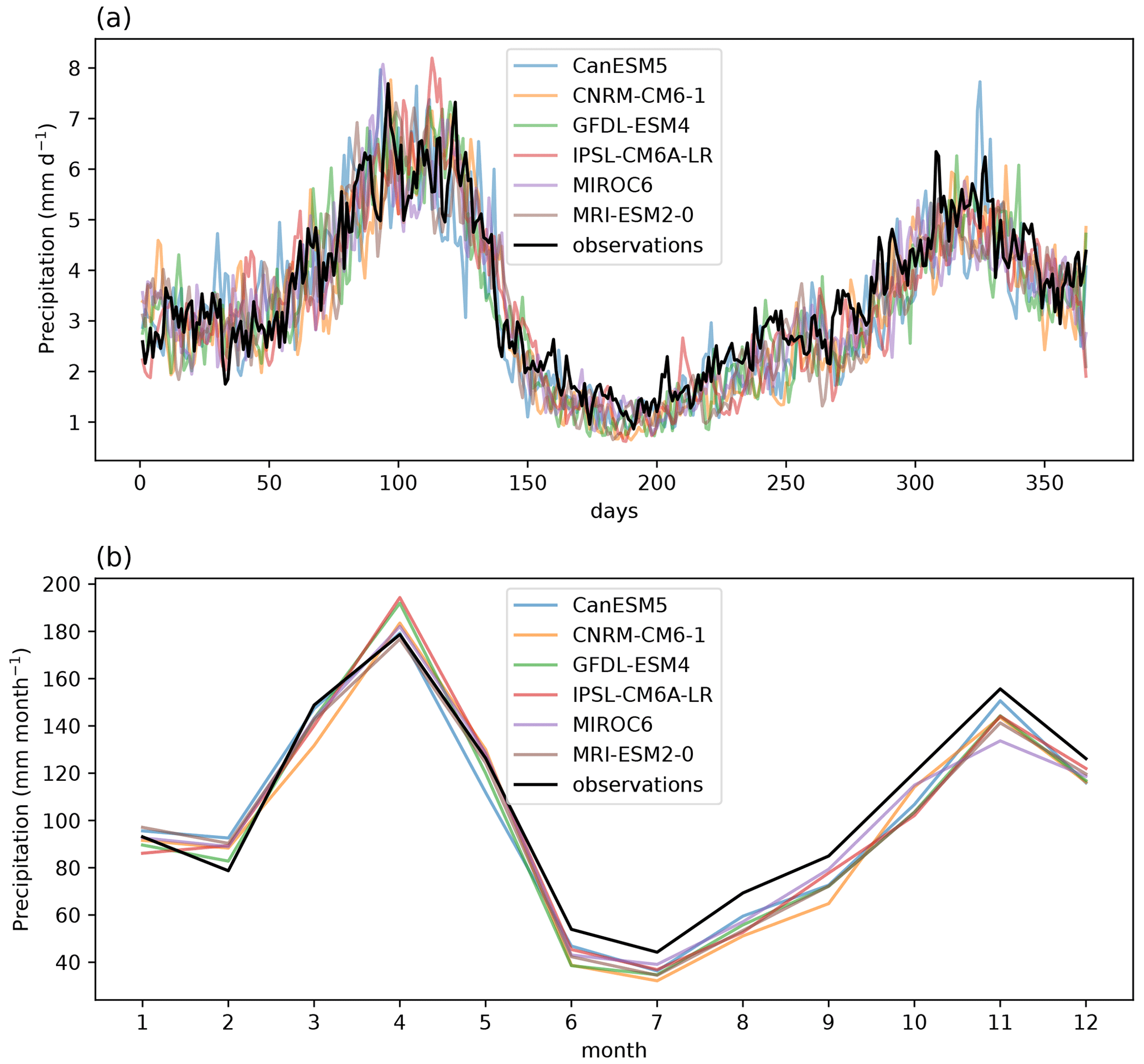
Figure C14Representation of seasonality of daily (a) and monthly precipitation (b) over Lake Victoria and its basin in observations (PERSIANN-CDR) and bias-adjusted GCMs (historical and SSP3-RCP7.0) evaluated in this study for the period 1985–2020.
All code necessary to run the water balance model and reproduce analyses is available here: https://github.com/VUB-HYDR/2024_Pietroiusti_etal_ESD (https://zenodo.org/doi/10.5281/zenodo.10794481, Pietroiusti, 2024). All non-restricted data necessary to reproduce the analysis are available on Zenodo: https://doi.org/10.5281/zenodo.10793917 (Pietroiusti et al., 2024). This repository contains data to run the water balance model, reproduced with permission from Vanderkelen et al. (2018; https://doi.org/10.5194/hess-22-5509-2018), i.e. lake evaporation data (originally from Thiery et al., 2015; https://doi.org/10.1175/JCLI-D-14-00565), information on land cover (originally from Mayaux et al., 2003; https://publications.jrc.ec.europa.eu/repository/handle/JRC24914), information on soil types (originally from Dewitte et al., 2013; https://doi.org/10.1016/j.geoderma.2013.07.007), basin and lake shapefiles (from Hamilton, 2016; https://doi.org/10.7910/DVN/PWFW26), and outflow data from Vanderkelen et al. (2018) updated with new in situ data by this study. The repository also contains data to reproduce the attribution analysis, i.e. observed GISTEMP GMST time series from NOAA (https://data.giss.nasa.gov/gistemp/, GISTEMP Team, 2024), GMST time series from ISIMIP3b bias-adjusted CMIP6 simulations from ISIMIP (https://doi.org/10.48364/ISIMIP.842396, Lange and Büchner, 2021), data on the IOD Dipole Mode Index (DMI) from NOAA (https://psl.noaa.gov/gcos_wgsp/Timeseries/DMI/, Saji, 2003), and lake level observations for the period 1948–1996 from Vanderkelen et al. (2018; https://doi.org/10.5194/hess-22-5509-2018) and from DAHITI since 1983 (https://dahiti.dgfi.tum.de/en/products/water-level-altimetry/, last access: 7 March 2022). The repository additionally includes output from the water balance model simulations performed in this study. Precipitation data are not included in the repository, but are freely available. Precipitation data from PERSIANN-CDR are available through NOAA (https://doi.org/10.7289/V51V5BWQ, Sorooshian et al., 2014). Bias-adjusted data from the CMIP6 climate models are available in the ISIMIP data repository (https://doi.org/10.48364/ISIMIP.842396.1, Lange and Büchner, 2021). The synthesis tool of the KNMI Climate Explorer is available here: https://climexp.knmi.nl/ (KNMI/WMO, 2024).
The supplement related to this article is available online at: https://doi.org/10.5194/esd-15-225-2024-supplement.
RP, IV, and WT designed the analysis. RP performed the analysis and wrote the manuscript. PB supervised the remote sensing analysis. MA provided data and contributed to discussions. CB and LT provided assistance regarding statistical analyses and contributed to discussions. FELO and NPMvL provided guidance and contributed to discussions. All authors provided guidance on the analysis and contributed to writing the manuscript.
The contact author has declared that none of the authors has any competing interests.
Publisher’s note: Copernicus Publications remains neutral with regard to jurisdictional claims made in the text, published maps, institutional affiliations, or any other geographical representation in this paper. While Copernicus Publications makes every effort to include appropriate place names, the final responsibility lies with the authors.
We are grateful to the Potsdam Institute for Climate Impact Research (PIK) for initiating and coordinating the ISIMIP initiative, with special thanks to Matthias Büchner for his oversight of ISIMIP data publishing and Stefan Lange for bias adjustment of CMIP6 data. We acknowledge the World Climate Research Programme, which, through its Working Group on Coupled Modelling coordinated and promoted CMIP6. We thank the climate modelling groups for producing and making their model output available, the Earth System Grid Federation (ESGF) for archiving the data and providing access, and the multiple funding agencies who support CMIP6 and ESGF. We acknowledge the work of World Weather Attribution in advancing extreme event attribution and thank its scientists, the WMO, and the KNMI for making attribution tools available through the Climate Explorer.
We thank the experts from LIST (Luxembourg), WASDI, RSS-Hydro, CIMA Foundation, and Terradue and in particular Marco Chini, Roberto Rudari, Lorenzo Alfieri, Paolo Campanella, Mauro Arcorace, and Laura Giustarini for their guidance and support regarding the remote sensing analysis and for providing access to the Earth Observation processing environments WASDI and GEP. We thank Faluku Nakulopa and Albert Nkwasa for discussion and insight into the flooding event. We thank Helen Houghton-Carr (UKCEH) for providing access to lake level observations from the late 1800s and Mary Akurut for providing data on lake levels and outflow for recent years (2020–2022).
Rosa Pietroiusti is supported by the VUB Research Council in the framework of a EUTOPIA inter-university co-tutelle PhD between the Vrije Universiteit Brussel, Belgium, and the University of Warwick, UK. The EUTOPIA alliance is part of the European Universities Initiatives co-funded by the European Union. She also acknowledges the support of the European Space Agency in providing the opportunity of a student internship in the Science, Applications and Climate Department of the Earth Observation Directorate at ESRIN, Frascati, Italy. The computational resources and services used in this work were provided by the VSC (Flemish Supercomputer Center), funded by the Research Foundation – Flanders (FWO) and the Flemish Government.
This research has been supported by the VUB research council (grant no. OZRIFTM12).
This paper was edited by Richard Betts and reviewed by two anonymous referees.
Akurut, M., Willems, P., and Niwagaba, C.: Potential Impacts of Climate Change on Precipitation over Lake Victoria, East Africa, in the 21st Century, Water, 6, 2634–2659, https://doi.org/10.3390/w6092634, 2014. a, b
Ashouri, H., Hsu, K. L., Sorooshian, S., Braithwaite, D. K., Knapp, K. R., Cecil, L. D., Nelson, B. R., and Prat, O. P.: PERSIANN-CDR: Daily Precipitation Climate Data Record from Multisatellite Observations for Hydrological and Climate Studies, Bull. Am. Meteorol. Soc., 96, 69–83, https://doi.org/10.1175/BAMS-D-13-00068.1, 2015. a
Ayugi, B., Zhihong, J., Zhu, H., Ngoma, H., Babaousmail, H., Rizwan, K., and Dike, V.: Comparison of CMIP6 and CMIP5 Models in Simulating Mean and Extreme Precipitation over East Africa, Int. J. Climatol., 41, 6474–6496, https://doi.org/10.1002/joc.7207, 2021. a
Beck, H. E., Wood, E. F., Pan, M., Fisher, C. K., Miralles, D. G., Van Dijk, A. I. J. M., McVicar, T. R., and Adler, R. F.: MSWEP V2 Global 3-Hourly 0.1° Precipitation: Methodology and Quantitative Assessment, Bull. Am. Meteorol. Soc., 100, 473–500, https://doi.org/10.1175/BAMS-D-17-0138.1, 2019. a
Black, E.: The Relationship between Indian Ocean Sea–Surface Temperature and East African Rainfall, Philos. T. R. Soc. A, 363, 43–47, https://doi.org/10.1098/rsta.2004.1474, 2005. a, b
Cai, W., Santoso, A., Wang, G., Weller, E., Wu, L., Ashok, K., Masumoto, Y., and Yamagata, T.: Increased Frequency of Extreme Indian Ocean Dipole Events Due to Greenhouse Warming, Nature, 510, 254–258, https://doi.org/10.1038/nature13327, 2014. a, b
Cai, W., Wang, G., Gan, B., Wu, L., Santoso, A., Lin, X., Chen, Z., Jia, F., and Yamagata, T.: Stabilised Frequency of Extreme Positive Indian Ocean Dipole under 1.5 °C Warming, Nat. Commun., 9, 4–11, https://doi.org/10.1038/s41467-018-03789-6, 2018. a, b, c, d
Chini, M., Hostache, R., Giustarini, L., and Matgen, P.: A Hierarchical Split-Based Approach for Parametric Thresholding of SAR Images: Flood Inundation as a Test Case, IEEE Trans. Geosci. Remote Sens., 55, 6975–6988, https://doi.org/10.1109/TGRS.2017.2737664, 2017. a, b, c, d
Chini, M., Pelich, R., Pulvirenti, L., Pierdicca, N., Hostache, R., and Matgen, P.: Sentinel-1 InSAR Coherence to Detect Floodwater in Urban Areas: Houston and Hurricane Harvey as a Test Case, Remote Sens., 11, 1–20, https://doi.org/10.3390/rs11020107, 2019. a
Chini, M., Pelich, R., Hostache, R., Matgen, P., Bossung, C., Campanella, P., Rudari, R., and Bally, P.: Systematic and Automatic Large-Scale Flood Monitoring System Using Sentinel-1 SAR Data, International Geoscience and Remote Sensing Symposium (IGARSS), 26 September 2020–2 October 2020, Waikoloa, HI, USA, 3251–3254, https://doi.org/10.1109/IGARSS39084.2020.9323428, 2020. a, b, c
Ciavarella, A., Cotterill, D., Stott, P., Kew, S., Philip, S., van Oldenborgh, G. J., Skålevåg, A., Lorenz, P., Robin, Y., Otto, F., Hauser, M., Seneviratne, S. I., Lehner, F., and Zolina, O.: Prolonged Siberian Heat of 2020 Almost Impossible without Human Influence, Climatic Change, 166, 9, https://doi.org/10.1007/s10584-021-03052-w, 2021. a
Coles, S.: An Introduction to Statistical Modeling of Extreme Values, Springer, London, ISBN: 978-1-84996-874-4, 2001. a, b
Conway, D., Allision, E., Felstead, R., and Goulden, M.: Rainfall Variability in East Africa: Implications for Natural Resources Management and Livelihoods, Philos. T. R. Soc. A, 363, 49–54, https://doi.org/10.1098/rsta.2004.1475, 2005. a
Cook, K. H., Fitzpatrick, R. G. J., Liu, W., and Vizy, E. K.: Seasonal Asymmetry of Equatorial East African Rainfall Projections: Understanding Differences between the Response of the Long Rains and the Short Rains to Increased Greenhouse Gases, Clim. Dynam., 55, 1759–1777, https://doi.org/10.1007/s00382-020-05350-y, 2020. a, b
Cucchi, M., Weedon, G. P., Amici, A., Bellouin, N., Lange, S., Müller Schmied, H., Hersbach, H., and Buontempo, C.: WFDE5: bias-adjusted ERA5 reanalysis data for impact studies, Earth Syst. Sci. Data, 12, 2097–2120, https://doi.org/10.5194/essd-12-2097-2020, 2020. a
Descheemaeker, K., Poesen, J., Borselli, L., Nyssen, J., Raes, D., Haile, M., Muys, B., and Deckers, J.: Runoff Curve Numbers for Steep Hillslopes with Natural Vegetation in Semi-Arid Tropical Highlands, Northern Ethiopia, Hydrol. Process., 22, 4097–4105, https://doi.org/10.1002/hyp.7011, 2008. a, b
Dewitte, O., Jones, A., Spaargaren, O., Breuning-Madsen, H., Brossard, M., Dampha, A., Deckers, J., Gallali, T., Hallett, S., Jones, R., Kilasara, M., Le Roux, P., Michéli, E., Montanarella, L., Thiombiano, L., Van Ranst, E., Yemefack, M., and Zougmore, R.: Harmonisation of the soil map of Africa at the continental scale, Geoderma, 211/212, 138–153, https://doi.org/10.1016/j.geoderma.2013.07.007, 2013.
Dunning, C. M., Black, E. C., and Allan, R. P.: The Onset and Cessation of Seasonal Rainfall over Africa, J. Geophys. Res., 121, 11405–11424, https://doi.org/10.1002/2016JD025428, 2016. a
Dunning, C. M., Black, E., and Allan, R. P.: Later Wet Seasons with More Intense Rainfall over Africa under Future Climate Change, J. Clim., 31, 9719–9738, https://doi.org/10.1175/JCLI-D-18-0102.1, 2018. a, b, c
Fahrland, E., Jacob, P., Schraser, H., and Kahabka, H.: Copernicus Digital Elevation Model: Product Handbook Version 3.0, 2020. a
Faranda, D., Vrac, M., Yiou, P., Jézéquel, A., and Thao, S.: Changes in Future Synoptic Circulation Patterns: Consequences for Extreme Event Attribution, Geophys. Res. Lett., 47, e2020GL088002, https://doi.org/10.1029/2020GL088002, 2020. a
Funk, C., Peterson, P., Landsfeld, M., Pedreros, D., Verdin, J., Shukla, S., Husak, G., Rowland, J., Harrison, L., Hoell, A., and Michaelsen, J.: The Climate Hazards Infrared Precipitation with Stations – A New Environmental Record for Monitoring Extremes, Sci. Data, 2, 1–21, https://doi.org/10.1038/sdata.2015.66, 2015. a
Funk, C., Harrison, L., Shukla, S., Korecha, D., Magadzire, T., Husak, G., Galu, G., and Hoell, A.: Assessing the Contributions of Local and East Pacific Warming to the 2015 Droughts in Ethiopia and Southern Africa, Bull. Am. Meteorol. Soc., 97, S75–S80, https://doi.org/10.1175/BAMS-D-16-0167.1, 2016. a
Funk, C., Pedreros, D., Nicholson, S., Hoell, A., Korecha, D., Galu, G., Artan, G., Segele, Z., Tadege, A., Atheru, Z., Teshome, F., Hailermariam, K., Harrison, L., and Pomposi, C.: Examining the Potential Contributions of Extreme “Western V” Sea Surface Temperatures to the 2017 March–June East African Drought, Bull. Am. Meteorol. Soc., 100, S55–S60, https://doi.org/10.1175/BAMS-D-18-0108.1, 2019. a
GISTEMP Team: GISS Surface Temperature Analysis (GISTEMP), version 4, NASA Goddard Institute for Space Studies [data set], https://data.giss.nasa.gov/gistemp/ (last access: 14 September 2021), 2024.
Global Climate Observing System Working Group on Surface Pressure: Dipole Mode Index (DMI), NOAA Physical Sciences Laboratory [data set], https://psl.noaa.gov/gcos_wgsp/Timeseries/DMI/ (last access: 7 March 2022), 2024.
Government of Kenya and UNDP: Rising Water Levels in Kenya's Rift Valley Lakes, Turkwel Gorge Dam and Lake Victoria, Tech. Rep., Govt. of Kenya and UNDP, https://ir-library.ku.ac.ke/handle/123456789/22851 (last access: 7 March 2024), 2021. a
Guha-Sapir, D., Below, R., and Hoyois, P.: EM-DAT: The CRED/OFDA International Disaster Database [data set], https://public.emdat.be/ (last access: 7 Mai 2021), 2022. a, b, c, d
Gulev, S., Thorne, P., Ahn, J., Dentener, F., Domingues, C., Gerland, Gong, D., Kaufman, D., Nnamchi, H., Quaas, J., Rivera, J., Sathyendranath, Smith, S., Trewin, B., von Schuckmann, K., and Vose, R.: Chap. 2: Changing State of the Climate System, in: Climate Change 2021: The Physical Science Basis, Contribution of Working Group I to the Sixth Assessment Report of the Intergovernmental Panel on Climate Change, edited by: Masson-Delmotte, V., Zhai, P., Pirani, A., Connors, S., Péan, C., Berger, S., Caud, N., Chen, Y., Goldfarb, L., Gomis, M., Huang, M., Leitzell, K., Lonnoy, E., Matthews, J., Maycock, T., Waterfield, T., Yelekçi, O., Yu, R., and Zhou, B., Cambridge University Press, Cambridge, United Kingdom and New York, NY, USA, 287–422, https://doi.org/10.1017/9781009157896, 2021. a
Hamilton, S.: Shoreline, Lake Victoria, vector polygon, Harvard Dataverse [data set], https://doi.org/10.7910/DVN/PWFW26, 2016.
Hammerling, D., Katzfuss, M., and Smith, R.: Climate Change Detection and Attribution, in: Handbook of Environmental and Ecological Statistics, edited by: Gelfand, A. E., Fuentes, M., Hoeting, J. A., and Smith, R. L., Chapman and Hall/CRC, Boca Raton, Taylor and Francis, ISBN 978-1-315-15250-9, https://doi.org/10.1201/9781315152509, 2019. a
Hansen, J., Ruedy, R., Sato, M., and Lo, K.: Global Surface Temperature Change, Rev. Geophys., 48, RG4004, https://doi.org/10.1029/2010RG000345, 2010. a
Joint Research Centre: Global Land Cover 2000 database (Africa), European Commission [data set], https://forobs.jrc.ec.europa.eu/glc2000/data (last access: 8 May 2018), 2003.
Kew, S. F., Philip, S. Y., Hauser, M., Hobbins, M., Wanders, N., van Oldenborgh, G. J., van der Wiel, K., Veldkamp, T. I. E., Kimutai, J., Funk, C., and Otto, F. E. L.: Impact of precipitation and increasing temperatures on drought trends in eastern Africa, Earth Syst. Dynam., 12, 17–35, https://doi.org/10.5194/esd-12-17-2021, 2021. a, b, c, d
Khaki, M. and Awange, J.: The 2019–2020 Rise in Lake Victoria Monitored from Space: Exploiting the State-of-the-Art Grace-Fo and the Newly Released Era-5 Reanalysis Products, Sensors, 21, 4304, https://doi.org/10.3390/s21134304, 2021. a, b, c
Kimutai, J., New, M., Wolski, P., and Otto, F.: Attribution of the Human Influence on Heavy Rainfall Associated with Flooding Events during the 2012, 2016, and 2018 March–April–May Seasons in Kenya, Weather Clim. Extrem., 38, 100529, https://doi.org/10.1016/j.wace.2022.100529, 2022. a, b
Kimutai, J., Barnes, C., Zachariah, M., Philip, S., Kew, S., Pinto, I., Wolski, P., Koren, G., Vecchi, G., Yang, W., Li, S, Vahlberg, Maja, Singh, R., Heinrich, D, Pereira, C., Arrighi, J., Thalheimer, L., Kane, C., and Otto, F. E. L.: Human-Induced Climate Change Increased Drought Severity in Horn of Africa, Tech. Rep., World Weather Attribution, Grantham Institute, Imperial College London, https://doi.org/10.25561/103482, 2023. a, b, c
Kite, G. W.: Recent Changes in Level of Lake Victoria, Hydrol. Sci. Bull., 26, 233–243, https://doi.org/10.1080/02626668109490883, 1981. a
KNMI/WMO: Climate Explorer, KNMI/WMO [software], https://climexp.knmi.nl/, last access: 7 March 2024.
Lake Victoria Basin Commission: Special Report on the Declining of Water Levels of Lake Victoria, 18 January 2006, East African Community Secretariat, Arusha, Tanzania, 2006. a
Lange, S.: Trend-preserving bias adjustment and statistical downscaling with ISIMIP3BASD (v1.0), Geosci. Model Dev., 12, 3055–3070, https://doi.org/10.5194/gmd-12-3055-2019, 2019a. a, b
Lange, S.: WFDE5 over land merged with ERA5 over the ocean (W5E5), V. 1.0. GFZ Data Services [data set], https://doi.org/10.5880/pik.2019.023, 2019b. a
Lange, S.: ISIMIP3b Bias Adjustment Fact Sheet Observational Dataset Bias Adjustment and Statistical Downscaling Method, https://www.isimip.org/gettingstarted/isimip3b-bias-adjustment/ (last access: 3 March 2024), 2020. a
Lange, S.: ISIMIP3BASD v2.5.0, Zenodo [code], https://doi.org/10.5281/zenodo.4686991, 2021. a, b
Lange, S. and Büchner, M.: ISIMIP3b bias-adjusted atmospheric climate input data (v1.1), ISIMIP Repository [data set], https://doi.org/10.48364/ISIMIP.842396.1, 2021.
Lenssen, N. J. L., Schmidt, G. A., Hansen, J. E., Menne, M. J., Persin, A., Ruedy, R., and Zyss, D.: Improvements in the GISTEMP Uncertainty Model, J. Geophys. Res.-Atmos., 124, 6307–6326, https://doi.org/10.1029/2018JD029522, 2019. a
Marthews, T. R., Jones, R. G., Dadson, S. J., Otto, F. E. L., Mitchell, D., Guillod, B. P., and Allen, M. R.: The Impact of Human-Induced Climate Change on Regional Drought in the Horn of Africa, J. Geophys. Res.-Atmos., 124, 4549–4566, https://doi.org/10.1029/2018JD030085, 2019. a, b
Mati, B. M., Mutie, S., Gadain, H., Home, P., and Mtalo, F.: Impacts of Land-use/Cover Changes on the Hydrology of the Transboundary Mara River, Kenya/Tanzania, Lakes & Reservoirs: Science, Policy and Management for Sustainable Use, 13, 169–177, https://doi.org/10.1111/j.1440-1770.2008.00367.x, 2008. a
Mayaux, P., Bartholomé, E., Massart, M., Cutsem, C. V., and Cabral, A.: A Land Cover Map of Africa, Tech. rep., European Commission Joint Research Center, Luxembourg, European Commission, ISBN: 92-894-5370-2, 2003. a
Mugo, R., Waswa, R., Nyaga, J. W., Ndubi, A., Adams, E. C., and Flores-Anderson, A. I.: Quantifying Land Use Land Cover Changes in the Lake Victoria Basin Using Satellite Remote Sensing: The Trends and Drivers between 1985 and 2014, Remote Sens., 12, 2829, https://doi.org/10.3390/rs12172829, 2020. a
Nicholson, S. E.: A Detailed Look at the Recent Drought Situation in the Greater Horn of Africa, J. Arid Environ., 103, 71–79, https://doi.org/10.1016/j.jaridenv.2013.12.003, 2014. a
Nicholson, S. E.: Long-Term Variability of the East African “short Rains” and Its Links to Large-Scale Factors, Int. J. Climatol., 35, 3979–3990, https://doi.org/10.1002/joc.4259, 2015. a
Nicholson, S. E.: Climate and Climatic Variability of Rainfall over Eastern Africa, Rev. Geophys., 55, 590–635, https://doi.org/10.1002/2016RG000544, 2017. a, b, c
Nicholson, S. E.: The ITCZ and the Seasonal Cycle over Equatorial Africa, Bull. Am. Meteorol. Soc., 99, 337–348, https://doi.org/10.1175/BAMS-D-16-0287.1, 2018. a
Nicholson, S. E. and Klotter, D. A.: Assessing the Reliability of Satellite and Reanalysis Estimates of Rainfall in Equatorial Africa, Remote Sens., 13, 3609, https://doi.org/10.3390/rs13183609, 2021. a
Nicholson, S. E., Fink, A. H., Funk, C., Klotter, D. A., and Satheesh, A. R.: Meteorological Causes of the Catastrophic Rains of October/November 2019 in Equatorial Africa, Glob. Planet. Change, 208, 103687, https://doi.org/10.1016/j.gloplacha.2021.103687, 2022. a, b, c
Olaka, L. A., Ogutu, J. O., Said, M. Y., and Oludhe, C.: Projected Climatic and Hydrologic Changes to Lake Victoria Basin Rivers under Three RCP Emission Scenarios for 2015–2100 and Impacts on the Water Sector, Water, 11, 1449, https://doi.org/10.3390/w11071449, 2019. a, b
Otto, F. E.: Extreme Events: The Art of Attribution, Nat. Clim. Change, 6, 342–343, https://doi.org/10.1038/nclimate2971, 2016. a
Otto, F. E.: Attribution of Weather and Climate Events, Ann. Rev. Environ. Resour., 42, 627–646, https://doi.org/10.1146/annurev-environ-102016-060847, 2017. a, b, c
Otto, F. E., Boyd, E., Jones, R. G., Cornforth, R. J., James, R., Parker, H. R., and Allen, M. R.: Attribution of Extreme Weather Events in Africa: A Preliminary Exploration of the Science and Policy Implications, Climatic Change, 132, 531–543, https://doi.org/10.1007/s10584-015-1432-0, 2015. a
Otto, F. E., Harrington, L., Schmitt, K., Philip, S., Kew, S., van Oldenborgh, G. J., Singh, R., Kimutai, J., and Wolski, P.: Challenges to Understanding Extreme Weather Changes in Lower Income Countries, Bull. Am. Meteorol. Soc., 101, E1851–E1860, https://doi.org/10.1175/BAMS-D-19-0317.1, 2020a. a
Otto, F. E., Harrington, L. J., Frame, D., Boyd, E., Lauta, K. C., Wehner, M., Clarke, B., Raju, E., Boda, C., Hauser, M., James, R. A., and Jones, R. G.: Toward an Inventory of the Impacts of Human-Induced Climate Change, Bull. Am. Meteorol. Soc., 101, E1972–E1979, https://doi.org/10.1175/BAMS-D-20-0027.1, 2020b. a
Otto, F. E. L.: Angry Weather: Heat Waves, Floods, Storms, and the New Science of Climate Change, Greystone Books, Vancouver/Berkeley, greystone books, ISBN: 978-1771646147, 2020. a
Otto, F. E. L., Philip, S., Kew, S., Li, S., King, A., and Cullen, H.: Attributing High-Impact Extreme Events across Timescales – a Case Study of Four Different Types of Events, Climatic Change, 149, 399–412, https://doi.org/10.1007/s10584-018-2258-3, 2018a. a
Otto, F. E. L., van der Wiel, K., van Oldenborgh, G. J., Philip, S., Kew, S. F., Uhe, P., and Cullen, H.: Climate Change Increases the Probability of Heavy Rains in Northern England/Southern Scotland like Those of Storm Desmond – a Real-Time Event Attribution Revisited, Environ. Res. Lett., 13, 024006, https://doi.org/10.1088/1748-9326/aa9663, 2018b. a
Pall, P., Aina, T., Stone, D. A., Stott, P. A., Nozawa, T., Hilberts, A. G., Lohmann, D., and Allen, M. R.: Anthropogenic Greenhouse Gas Contribution to Flood Risk in England and Wales in Autumn 2000, Nature, 470, 382–385, https://doi.org/10.1038/nature09762, 2011. a
Palmer, P. I., Wainwright, C. M., Dong, B., Maidment, R. I., Wheeler, K. G., Gedney, N., Hickman, J. E., Madani, N., Folwell, S. S., Abdo, G., Allan, R. P., Black, E. C. L., Feng, L., Gudoshava, M., Haines, K., Huntingford, C., Kilavi, M., Lunt, M. F., Shaaban, A., and Turner, A. G.: Drivers and Impacts of Eastern African Rainfall Variability, Nat. Rev. Earth Environ., 4, 254–270, https://doi.org/10.1038/s43017-023-00397-x, 2023. a, b, c, d, e
Philip, S., Kew, S. F., van Oldenborgh, G. J., Aalbers, E., Vautard, R., Otto, F., Haustein, K., Habets, F., and Singh, R.: Validation of a Rapid Attribution of the May/June 2016 Flood-Inducing Precipitation in France to Climate Change, J. Hydrometeorol., 19, 1881–1898, https://doi.org/10.1175/JHM-D-18-0074.1, 2018a. a
Philip, S., Kew, S. F., van Oldenborgh, G. J., Otto, F., O'Keefe, S., Haustein, K., King, A., Zegeye, A., Eshetu, Z., Hailemariam, K., Singh, R., Jjemba, E., Funk, C., and Cullen, H.: Attribution Analysis of the Ethiopian Drought of 2015, J. Clim., 31, 2465–2486, https://doi.org/10.1175/JCLI-D-17-0274.1, 2018b. a, b, c, d, e
Philip, S., Sparrow, S., Kew, S. F., van der Wiel, K., Wanders, N., Singh, R., Hassan, A., Mohammed, K., Javid, H., Haustein, K., Otto, F. E. L., Hirpa, F., Rimi, R. H., Islam, A. K. M. S., Wallom, D. C. H., and van Oldenborgh, G. J.: Attributing the 2017 Bangladesh floods from meteorological and hydrological perspectives, Hydrol. Earth Syst. Sci., 23, 1409–1429, https://doi.org/10.5194/hess-23-1409-2019, 2019. a
Philip, S., Kew, S., van Oldenborgh, G. J., Otto, F., Vautard, R., van der Wiel, K., King, A., Lott, F., Arrighi, J., Singh, R., and van Aalst, M.: A protocol for probabilistic extreme event attribution analyses, Adv. Stat. Clim. Meteorol. Oceanogr., 6, 177–203, https://doi.org/10.5194/ascmo-6-177-2020, 2020. a, b, c, d, e, f, g, h, i, j, k, l
Pietroiusti, R.: VUB-HYDR/2024_Pietroiusti_etal_ESD: Release of Lake Victoria Python water balance model and analysis scripts (v1.0), Zenodo [code], https://doi.org/10.5281/zenodo.10794482, 2024.
Pietroiusti, R., Vanderkelen, I., Otto, F. E. L., Barnes, C., Temple, L., Akurut, M., Bally, P., van Lipzig, N. P. M., and Thiery, W.: Data used in Pietroiusti et al. 2024 ESD, Zenodo [data set], https://doi.org/10.5281/zenodo.10793917, 2024.
Rowell, D. P., Booth, B. B., Nicholson, S. E., and Good, P.: Reconciling Past and Future Rainfall Trends over East Africa, J. Clim., 28, 9768–9788, https://doi.org/10.1175/JCLI-D-15-0140.1, 2015. a, b, c, d, e
Saji, N. H. and Yamagata, T.: Possible impacts of Indian Ocean Dipole mode events on global climate, Clim. Res., 25, 151–169, 2003.
Salih, A. A. M., Baraibar, M., Mwangi, K. K., and Artan, G.: Climate Change and Locust Outbreak in East Africa, Nat. Clim. Change, 10, 584–585, https://doi.org/10.1038/s41558-020-0835-8, 2020. a
Schaller, N., Kay, A. L., Lamb, R., Massey, N. R., van Oldenborgh, G. J., Otto, F. E. L., Sparrow, S. N., Vautard, R., Yiou, P., Ashpole, I., Bowery, A., Crooks, S. M., Haustein, K., Huntingford, C., Ingram, W. J., Jones, R. G., Legg, T., Miller, J., Skeggs, J., Wallom, D., Weisheimer, A., Wilson, S., Stott, P. A., and Allen, M. R.: Human Influence on Climate in the 2014 Southern England Winter Floods and Their Impacts, Nat. Clim. Change, 6, 627–634, https://doi.org/10.1038/nclimate2927, 2016. a
Schwatke, C., Dettmering, D., Bosch, W., and Seitz, F.: DAHITI– an innovative approach for estimating water level time series over inland waters using multi-mission satellite altimetry, Hydrol. Earth Syst. Sci., 19, 4345–4364, https://doi.org/10.5194/hess-19-4345-2015, 2015.
Seager, R., Cane, M., Henderson, N., Lee, D.-E., Abernathey, R., and Zhang, H.: Strengthening Tropical Pacific Zonal Sea Surface Temperature Gradient Consistent with Rising Greenhouse Gases, Nat. Clim. Change, 9, 517–522, https://doi.org/10.1038/s41558-019-0505-x, 2019. a
Sene, K., Houghton Carr, H., and Tych, W.: Reflections on almost a century of hydrological studies on Africa's largest lake, Proc. IAHS, 384, 141–147, https://doi.org/10.5194/piahs-384-141-2021, 2021. a, b, c, d, e
Sene, K. J.: Theoretical Estimates for the Influence of Lake Victoria on Flows in the Upper White Nile, Hydrol. Sci. J., 45, 125–145, https://doi.org/10.1080/02626660009492310, 2000. a, b
Shepherd, T. G.: Atmospheric Circulation as a Source of Uncertainty in Climate Change Projections, Nat. Geosci., 7, 703–708, https://doi.org/10.1038/NGEO2253, 2014. a
Shepherd, T. G.: A Common Framework for Approaches to Extreme Event Attribution, Curr. Clim. Change Rep., 2, 28–38, https://doi.org/10.1007/s40641-016-0033-y, 2016. a, b, c
Shepherd, T. G.: Storyline Approach to the Construction of Regional Climate Change Information, P. Roy. Soc. A, 475, 20190013, https://doi.org/10.1098/rspa.2019.0013, 2019. a
Shepherd, T. G.: Bringing Physical Reasoning into Statistical Practice in Climate-Change Science, Climatic Change, 169, 1–19, https://doi.org/10.1007/s10584-021-03226-6, 2021. a, b
Sorooshian, S., Hsu, K., Braithwaite, D., Ashouri, H., and NOAA CDR Program: NOAA Climate Data Record (CDR) of Precipitation Estimation from Remotely Sensed Information using Artificial Neural Networks (PERSIANN-CDR), Version 1 Revision 1. [1983–2020], NOAA National Centers for Environmental Information [data set], https://doi.org/10.7289/V51V5BWQ, 2014.
Souverijns, N., Thiery, W., Demuzere, M., and Lipzig, N. P. M. V.: Drivers of Future Changes in East African Precipitation, Environ. Res. Lett., 11, 114011, https://doi.org/10.1088/1748-9326/11/11/114011, 2016. a, b, c
Stevens, F. R., Gaughan, A. E., Linard, C., and Tatem, A. J.: Disaggregating Census Data for Population Mapping Using Random Forests with Remotely-Sensed and Ancillary Data, PLoS ONE, 10, 1–22, https://doi.org/10.1371/journal.pone.0107042, 2015. a
Stone, D. A., Christidis, N., Folland, C., Perkins-Kirkpatrick, S., Perlwitz, J., Shiogama, H., Wehner, M. F., Wolski, P., Cholia, S., Krishnan, H., Murray, D., Angélil, O., Beyerle, U., Ciavarella, A., Dittus, A., Quan, X.-W., and Tadross, M.: Experiment Design of the International CLIVAR C20C+ Detection and Attribution Project, Weather Clim. Extrem., 24, 100206, https://doi.org/10.1016/j.wace.2019.100206, 2019. a
Sutcliffe, J. V. and Petersen, G.: Lake Victoria: Derivation of a Corrected Natural Water Level Series, Hydrol. Sci. J., 52, 1316–1321, https://doi.org/10.1623/hysj.52.6.1316, 2007. a, b
Technical University Munich: Database for Hydrological Time Series over Inland Waters (DAHITI) [data set], http://dahiti.dgfi.tum.de, last access: 7 March 2022.
Thiery, W., Davin, E. L., Panitz, H. J., Demuzere, M., Lhermitte, S., and Van Lipzig, N.: The Impact of the African Great Lakes on the Regional Climate, J. Clim., 28, 4061–4085, https://doi.org/10.1175/JCLI-D-14-00565.1, 2015. a, b
Thiery, W., Davin, E. L., Seneviratne, S. I., Bedka, K., Lhermitte, S., and van Lipzig, N. P. M.: Hazardous Thunderstorm Intensification over Lake Victoria, Nat. Commun., 7, 12786, https://doi.org/10.1038/ncomms12786, 2016. a, b, c
Thiery, W., Gudmundsson, L., Bedka, K., Semazzi, F. H. M., Lhermitte, S., Willems, P., van Lipzig, N. P. M., and Seneviratne, S. I.: Early Warnings of Hazardous Thunderstorms over Lake Victoria, Environ. Res. Lett., 12, 074012, https://doi.org/10.1088/1748-9326/aa7521, 2017. a
Uhe, P., Philip, S., Kew, S., Shah, K., Kimutai, J., Mwangi, E., van Oldenborgh, G. J., Singh, R., Arrighi, J., Jjemba, E., Cullen, H., and Otto, F.: Attributing Drivers of the 2016 Kenyan Drought, Int. J. Climatol., 38, e554–e568, https://doi.org/10.1002/joc.5389, 2018. a
Ummenhofer, C. C., Gupta, A. S., England, M. H., and Reason, C. J.: Contributions of Indian Ocean Sea Surface Temperatures to Enhanced East African Rainfall, J. Clim., 22, 993–1013, https://doi.org/10.1175/2008JCLI2493.1, 2009. a, b
USDA-SCS: Chapter 10: Estimation of Direct Runoff from Storm Rainfall, in: Hydrology National Engineering Handbook, United States Department of Agriculture, https://directives.sc.egov.usda.gov/17752.wba (last access: 12 March 2024), 2004. a, b, c
Van de Walle, J., Thiery, W., Brousse, O., Souverijns, N., Demuzere, M., and van Lipzig, N. P.: A Convection-Permitting Model for the Lake Victoria Basin: Evaluation and Insight into the Mesoscale versus Synoptic Atmospheric Dynamics, Clim. Dynam., 54, 1779–1799, https://doi.org/10.1007/s00382-019-05088-2, 2020. a, b
Van de Walle, J., Thiery, W., Brogli, R., Martius, O., Zscheischler, J., and van Lipzig, N. P.: Future Intensification of Precipitation and Wind Gust Associated Thunderstorms over Lake Victoria, Weather Clim. Extrem., 34, 100391, https://doi.org/10.1016/j.wace.2021.100391, 2021. a
Van Lipzig, N. P. M., Walle, J. V. D., Belušić, D., Berthou, S., Coppola, E., Demuzere, M., Fink, A. H., Finney, D. L., Glazer, R., Ludwig, P., Marsham, J. H., Nikulin, G., Pinto, J. G., Rowell, D. P., Wu, M., and Thiery, W.: Representation of Precipitation and Top-of-Atmosphere Radiation in a Multi-Model Convection-Permitting Ensemble for the Lake Victoria Basin (East-Africa), Clim. Dynam., 60, 4033–4054, https://doi.org/10.1007/s00382-022-06541-5, 2023. a
van Oldenborgh, G. J., Krikken, F., Lewis, S., Leach, N. J., Lehner, F., Saunders, K. R., van Weele, M., Haustein, K., Li, S., Wallom, D., Sparrow, S., Arrighi, J., Singh, R. K., van Aalst, M. K., Philip, S. Y., Vautard, R., and Otto, F. E. L.: Attribution of the Australian bushfire risk to anthropogenic climate change, Nat. Hazards Earth Syst. Sci., 21, 941–960, https://doi.org/10.5194/nhess-21-941-2021, 2021. a
van Oldenborgh, G. J., van der Wiel, K., Kew, S., Philip, S., Otto, F., Vautard, R., King, A., Lott, F., Arrighi, J., Singh, R., and van Aalst, M.: Pathways and Pitfalls in Extreme Event Attribution, Climatic Change, 166, 1–27, https://doi.org/10.1007/s10584-021-03071-7, 2021. a, b
Vanderkelen, I.: Projecting the Future Levels of Lake Victoria, M.Sc. thesis, KU Leuven/Vrije Universiteit Brussel, ISSN 0012-3692, 2016. a
Vanderkelen, I., van Lipzig, N. P. M., and Thiery, W.: Modelling the water balance of Lake Victoria (East Africa) – Part 1: Observational analysis, Hydrol. Earth Syst. Sci., 22, 5509–5525, https://doi.org/10.5194/hess-22-5509-2018, 2018a. a, b, c, d, e, f, g, h, i, j, k, l, m, n, o, p, q
Vanderkelen, I., van Lipzig, N. P. M., and Thiery, W.: Modelling the water balance of Lake Victoria (East Africa) – Part 2: Future projections, Hydrol. Earth Syst. Sci., 22, 5527–5549, https://doi.org/10.5194/hess-22-5527-2018, 2018. a, b
Wainwright, C. M., Marsham, J. H., Keane, R. J., Rowell, D. P., Finney, D. L., Black, E., and Allan, R. P.: “Eastern African Paradox” Rainfall Decline Due to Shorter Not Less Intense Long Rains, npj Clim. Atmos. Sci., 2, 1–9, https://doi.org/10.1038/s41612-019-0091-7, 2019. a, b, c, d, e
Wainwright, C. M., Finney, D. L., Kilavi, M., Black, E., and Marsham, J. H.: Extreme Rainfall in East Africa, October 2019–January 2020 and Context under Future Climate Change, Weather, 76, 26–31, https://doi.org/10.1002/wea.3824, 2021a. a, b, c, d, e, f, g
Wainwright, C. M., Marsham, J. H., Rowell, D. P., Finney, D. L., and Black, E.: Future Changes in Seasonality in East Africa from Regional Simulations with Explicit and Parameterized Convection, J. Clim., 34, 1367–1385, https://doi.org/10.1175/JCLI-D-20-0450.1, 2021b. a
WMO, APFM, and Ministry of Water Resources Management and Development: Strategy for Flood Management for Lake Victoria, Kenya, Tech. Rep., World Meteorological Organization (WMO) and Ministry of Water Resources Management and Development, Kenya, https://www.floodmanagement.info/3 (last access: 12 March 2024), 2004. a
WMO-UNDP: Hydrometeorological Survey of the Catchments of Lakes Victoria, Kyoga and Albert: Vol. 1 Meteorology and Hydrology of the Basin, WMO, https://library.wmo.int/records/item (last access: 12 March 2024), 1974. a
WorldPop: WorldPop and Center for International Earth Science Information Network (CIESIN), Columbia University (2018), Global High Resolution Population Denominators Project – Funded by The Bill and Melinda Gates Foundation (OPP1134076), https://doi.org/10.5258/SOTON/WP00645, 2018. a
https://reliefweb.int/map/somalia/, last access: 1 March 2024.
https://reliefweb.int/report/ethiopia/, last access: 1 March 2024, https://www.theeastafrican.co.ke/tea/news/, last access: 1 March 2024, https://floodlist.com/africa/kenya-floods-north-central-regions-may-2020, last access: 1 March 2024, https://floodlist.com/africa/rwanda-floods-07-may-2020, last access: 1 March 2024, https://floodlist.com/africa/uganda-floods-kampala-september-2020, last access: 1 March 2024.
https://reliefweb.int/report/world/, last access: 1 March 2024
https://reliefweb.int/report/kenya/, last access: 1 March 2024.
https://reliefweb.int/report/united-republic-tanzania/, last access: 1 March 2024.
https://www.reuters.com/article/, last access: 1 March 2024.
https://www.monitor.co.ug/News/National/, last access: 1 March 2024.
https://www.theguardian.com/global-development/2020/, last access: 1 March 2024, https://theconversation.com/lake-victoria-could-burst, last access: 1 March 2024.
Wikipedia, https://en.wikipedia.org/wiki/2020, last access: 1 March 2024.
https://reliefweb.int/map/somalia/, last access: 1 March 2024.
NTV Kenya (3 May 2020), https://www.youtube.com/watch?v=i906ouUW-hw, last access: 1 March 2024.
UN OCHA (7 May 2020), https://reliefweb.int/disaster/fl-2020-000128-ken, last access: 1 March 2024.
Reuters (19 August 2020), https://news.trust.org/item/20200819141141-rb3c8, last access: 1 March 2024.
Floodlist (22 October 2020), https://floodlist.com/africa/kenya-lake-turkana-floods-october-2020, last access: 1 March 2024.
The Nation (6 January 2021), https://nation.africa/kenya/counties/homa-bay/, last access: 1 March 2024.
East Africa Institute (26 May 2020), https://www.youtube.com/watch?v=DBbHZS8LTzE, last access: 1 March 2024.
The Daily Monitor (1 May 2020), https://www.monitor.co.ug/uganda/news/, last access: 1 March 2024.
Floodlist (4 May 2020), https://floodlist.com/africa/uganda-floods-western-northern-region-may-2020, last access: 1 March 2024.
IFRC (8 May 2020), https://reliefweb.int/report/united-republic-tanzania/, last access: 1 March 2024.
- Abstract
- Introduction
- Data and methods
- Results
- Discussion
- Conclusions
- Appendix A: Appendix tables
- Appendix B: Appendix text
- Appendix C: Appendix figures
- Code and data availability
- Author contributions
- Competing interests
- Disclaimer
- Acknowledgements
- Financial support
- Review statement
- References
- Supplement