Sea-ice thermodynamics can determine waterbelt scenarios for Snowball Earth

Snowball Earth refers to multiple periods in the Neoproterozoic during which geological evidence indicates that the Earth was largely covered in ice. A Snowball Earth results from a runaway ice–albedo feedback, but there is an ongoing debate about how the feedback stopped: with fully ice-covered oceans or with a narrow strip of open water around the Equator. The latter states are called waterbelt states and are an attractive explanation for Snowball Earth events because they provide a refugium for the survival of photosynthetic aquatic life, while still explaining Neoproterozoic geology. Waterbelt states can be stabilized by bare sea ice in the subtropical desert regions, which lowers the surface albedo and stops the runaway ice–albedo feedback. However, the choice of sea-ice model in climate simulations significantly impacts snow cover on ice and, consequently, surface albedo.

Here, we investigate the robustness of waterbelt states with respect to the thermodynamical representation of sea ice. We compare two thermodynamical sea-ice models, an idealized zero-layer Semtner model, in which sea ice is always in equilibrium with the atmosphere and ocean, and a three-layer Winton model that is more sophisticated and takes into account the heat capacity of ice. We deploy the global icosahedral non-hydrostatic atmospheric (ICON-A) model in an idealized aquaplanet setup and calculate a comprehensive set of simulations to determine the extent of the waterbelt hysteresis. We find that the thermodynamic representation of sea ice strongly influences snow cover on sea ice over the range of all simulated climate states. Including heat capacity by using the three-layer Winton model increases snow cover and enhances the ice–albedo feedback. The waterbelt hysteresis found for the zero-layer model disappears in the three-layer model, and no stable waterbelt states are found. This questions the relevance of a subtropical bare sea-ice region for waterbelt states and might help explain drastically varying model results on waterbelt states in the literature.

1 Introduction

The Neoproterozoic glaciations are commonly assumed to be of global extent and have become known under the term “Snowball Earth” (Kirschvink, 1992; Hoffman and Schrag, 2002). A Snowball Earth is initiated by a runaway ice–albedo feedback, where expanding ice, increasing planetary albedo and falling global temperatures compose a feedback loop that leads to rapid glaciation until the Earth is either fully ice-covered or the feedback is stopped by some other stabilizing mechanism (Pierrehumbert et al., 2011).

Climate states where the runaway ice–albedo feedback is stopped with a stable ice border equatorward of 30° have been termed soft Snowball (Hyde et al., 2000; Yang et al., 2012a, b) or waterbelt states (Abbot et al., 2011; Rose, 2015; Brunetti et al., 2019; Ragon et al., 2022; Braun et al., 2022). For waterbelt states to be a feasible explanation for the Cryogenian glaciations, they have to be accessible from a temperate climate state, and they have to be stable over a large range of atmospheric CO₂, as only then can they explain the long duration of the Snowball event and the survival of photosynthetic aquatic life (Hoffman et al., 2017). Two major effects have been shown to allow states with low-latitude ice margins: firstly, heat convergence at the sea-ice margin stopping ice growth thanks to the ocean circulation (Rose, 2015) and, secondly, bare low-albedo sea ice in the subtropics stopping the ice–albedo feedback (Abbot et al., 2011). Here we focus on the latter effect, the Jormungand mechanism.

The Jormungand mechanism is based on the assumption that sea ice will not be covered by snow when it reaches the subtropics, where the descending branch of the Hadley circulation results in net sublimation and evaporation. Consequently, snow melts, and a larger region of darker bare sea ice is exposed, weakening the ice–albedo feedback until a stable state is reached. We refer to this region at the ice margin as the bare sea-ice region (BASIR) in this study. For the BASIR to have an impact on the climate, a strong albedo contrast between dark bare sea ice and bright snow is required (Warren et al., 2002; Dadic et al., 2013). The width of the BASIR then governs the strength of the Jormungand mechanism.

In this study, we assess the robustness of the Jormungand mechanism by examining sea ice and its snow cover in two different thermodynamical sea-ice models. That is, we ask the following question: how robust is the Jormungand mechanism when using different sea-ice schemes? Recently, Braun et al. (2022) also postulated a strong influence of subtropical clouds on waterbelt stability, as the optical thickness of subtropical clouds determines the strength of the ice–albedo feedback when ice grows beneath the clouds. The stabilizing effect of clouds over ice is an overarching effect, as clouds mute the ice–albedo feedback. Here, however, we isolate the effect of the sea-ice scheme on the ice–albedo feedback.

Abbot et al. (2010) showed that using more sea-ice layers generally reduces surface melting by reducing the “melt-ratchet” effect. This is because simple thermodynamic sea-ice models overestimate the daily and seasonal cycle of surface temperature and consequently overestimate surface melting (Semtner, 1984). Specifically for Snowball Earth initiation, using a three-layer sea-ice model instead of a zero-layer sea-ice model results in stronger ice–albedo feedback because the decreased surface melting results in larger ice cover and more snow on ice (Hörner et al., 2022). This results in easier Snowball Earth initiation with a tipping point that is located at 50 % higher CO₂ content. In this study, we will extend the results of Hörner et al. (2022) and demonstrate that the same mechanism also influences waterbelt states. Waterbelt states that are stable and accessible using the simple zero-layer model are destabilized and absent when the more sophisticated three-layer model is used.

This paper is structured as follows. In Sect. 2, the methods and the model setup are described. Section 3 presents the impacts of the different sea-ice schemes on the ice–albedo feedback and the waterbelt states. Section 4 discusses the implications for waterbelt states found previously in different climate models and provides a conclusion.

2 Methods

2.1 ICON-A

We deploy the icosahedral non-hydrostatic atmospheric (ICON-A) model (Giorgetta et al., 2018). There have been multiple studies on Snowball climate using the ICON model (e.g., Braun et al., 2022; Hörner et al., 2022; Ramme and Marotzke, 2022). Its predecessor ECHAM, which to a large extent uses the same physics package (Giorgetta et al., 2018), has also been used in Snowball Earth simulations (e.g., Marotzke and Botzet, 2007; Voigt and Abbot, 2012; Abbot et al., 2012), including studies of waterbelt states (Abbot et al., 2011; Voigt et al., 2011).

The model and model setup are the same as in Hörner et al. (2022) and Braun et al. (2022). We use ICON-A with an effective horizontal resolution of 160 km and 45 atmospheric vertical levels. ICON-A is coupled to a mixed-layer ocean of 50 m depth without any horizontal heat transport to simulate an aquaplanet without continents. A circular Kepler orbit and a solar constant reduced to 1285 W m⁻², as well as an idealized 360 d year, are applied to represent Neoproterozoic boundary conditions (Gough, 1981). The albedo for cold snow and ice is 0.79 and 0.45, respectively. These values are linearly decreased to 0.66 for warm snow and 0.38 for warm ice, starting from 1 K below melting temperature.

The value of bare-ice albedo is at the lower end of the range suggested by observations (Dadic et al., 2013; Webster and Warren, 2022). Consequently, our choice of albedo values works in favor of a stable waterbelt state because of the large albedo difference between snow and bare ice. The main reason for our choice is to ensure comparability with the previous studies of Braun et al. (2022), Hörner et al. (2022) and Abbot et al. (2011), which employed precisely the same albedo values. Overall, the model setup follows Abbot et al. (2011), who first postulated the Jormungand state in idealized aquaplanet slab–ocean simulations with varying longwave forcing using the CAM and ECHAM models. Following Braun et al. (2022), we adapt the cloud scheme to allow ICON-A to simulate stable waterbelt states.

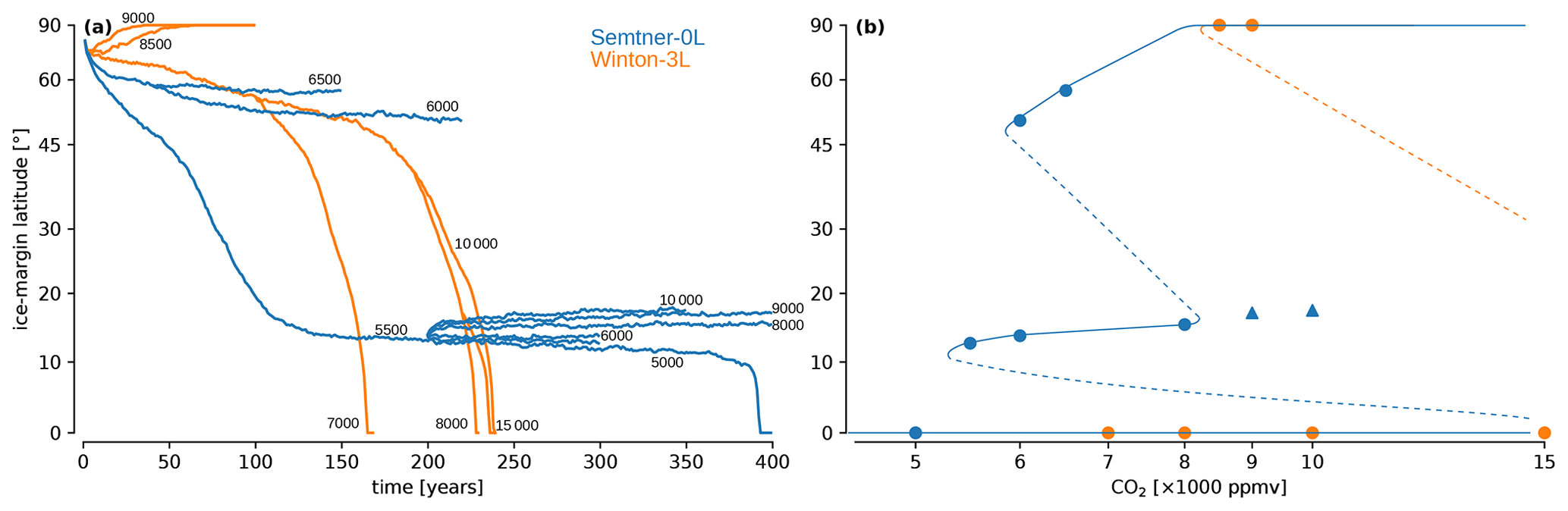
Figure 1 (a) Evolution of the yearly mean ice-margin latitude for simulations with Semtner-0L (blue) and Winton-3L (orange). Each line is labeled with its atmospheric CO₂ content in units of parts per million by volume (ppmv). (b) Estimated bifurcation diagrams. For equilibrated simulations, the ice-margin latitude is shown by solid circles. Simulations that continuously drift in snow cover are expected to melt and are depicted by upward-pointing triangles. Solid lines indicate the branches of stable equilibrium states, while dashed lines are for unstable equilibrium states. The exact positions of the tipping point and the branches of the unstable states are uncertain and should be considered best guesses.

We compare simulations with two different sea-ice schemes: the Semtner zero-layer scheme (Semtner, 1976), hereafter Semtner-0L, and the Winton three-layer scheme (Winton, 2000), hereafter Winton-3L. Semtner-0L only considers surface temperature and does not predict internal ice temperatures. This means that the heat capacity of ice and brine pockets is neglected. Winton-3L, on the other hand, takes into account the heat capacity. The model follows the energy-conserving approach of Bitz and Lipscomb (1999) and predicts ice temperatures at two internal levels and at the surface. Energy stored in brine pockets is considered through a temperature-dependent enthalpy of fusion for ice. In the case of bare ice, Winton-3L allows a portion of incoming solar radiation to penetrate the ice. In both models, snow is converted to ice when the snow cover is submerged below the water level. For a more in-depth comparison of the ice models in the context of Snowball Earth initiation, we refer the reader to Hörner et al. (2022).

ICON-A tends to become more unstable in colder climates. We therefore decrease the time step from the initial 10 to 8 min and finally to 6 min. All stable simulations on the temperate branch of the bifurcation diagram use a time step of 10 min, and the waterbelt and Snowball Earth branches use a time step of 6 min (see Fig. 1). As in Ramme and Marotzke (2022), we increase the Rayleigh damping in the uppermost levels of the atmosphere for time steps smaller than 10 min (Klemp et al., 2008).

2.2 Simulation design

Two sets of simulations are performed: one using the Semtner-0L model (Semtner, 1976) and the other using the Winton-3L model (Winton, 2000). Each simulation is characterized by its constant atmospheric CO₂ content and its initial condition. Most simulations are started from ice-free initial conditions, with sea-surface temperatures (SSTs) derived from AMIP runs of the present-day climate. The initial SST profile is zonally symmetric and symmetric with respect to the Equator. The global average SST is 291 K, ranging from 273 K at the poles to 301 K at the Equator. Some simulations are branched off from other simulations after a certain ice-margin latitude has been reached. In these cases, a new simulation with a different constant atmospheric CO₂ content is started from a restart file of the parent simulation. This is done to find potentially hidden waterbelt states, to determine the width of the waterbelt hysteresis in the bifurcation diagram and to save computing time.

3 Results

3.1 Simulation overview

Stable waterbelt states are found with the zero-layer Semtner sea-ice model but not with the three-layer Winton model. Figure 1a shows the evolution of the ice margin for all simulations. All Winton-3L simulations either stay at an ice-free state or fall into a Snowball state in less than 250 years. Semtner-0L, in contrast, results in a waterbelt state when starting from ice-free initial conditions with a CO₂ content of 5500 ppmv. From there, more simulations are branched off with different CO₂ content to assess the width of the waterbelt hysteresis.

A best guess of the bifurcation diagram is constructed from these simulations in Fig. 1b. The waterbelt hysteresis in Semtner-0L extends over a range of CO₂ from 5500 to 8000 ppmv. The Semtner-0L bifurcation diagram is the same as in Braun et al. (2022) (their Fig. 1a), since we are using the same model and model setup. In Winton-3L no waterbelt state is found up to a CO₂ value of 15 000 ppmv. We cannot formally exclude the possibility of a hidden waterbelt state at even higher values of CO₂ forcing. However, even if such a state existed, it would be geologically irrelevant because it would be inaccessible from a temperate state. The atmospheric CO₂ to reach that state would be much higher than that of the tipping point of Snowball Earth initiation (between 8000 and 8500 ppmv). Additionally, the strong ice–albedo feedback in Winton-3L for a low-latitude ice margin (see Sect. 3.4) makes such a state unlikely.

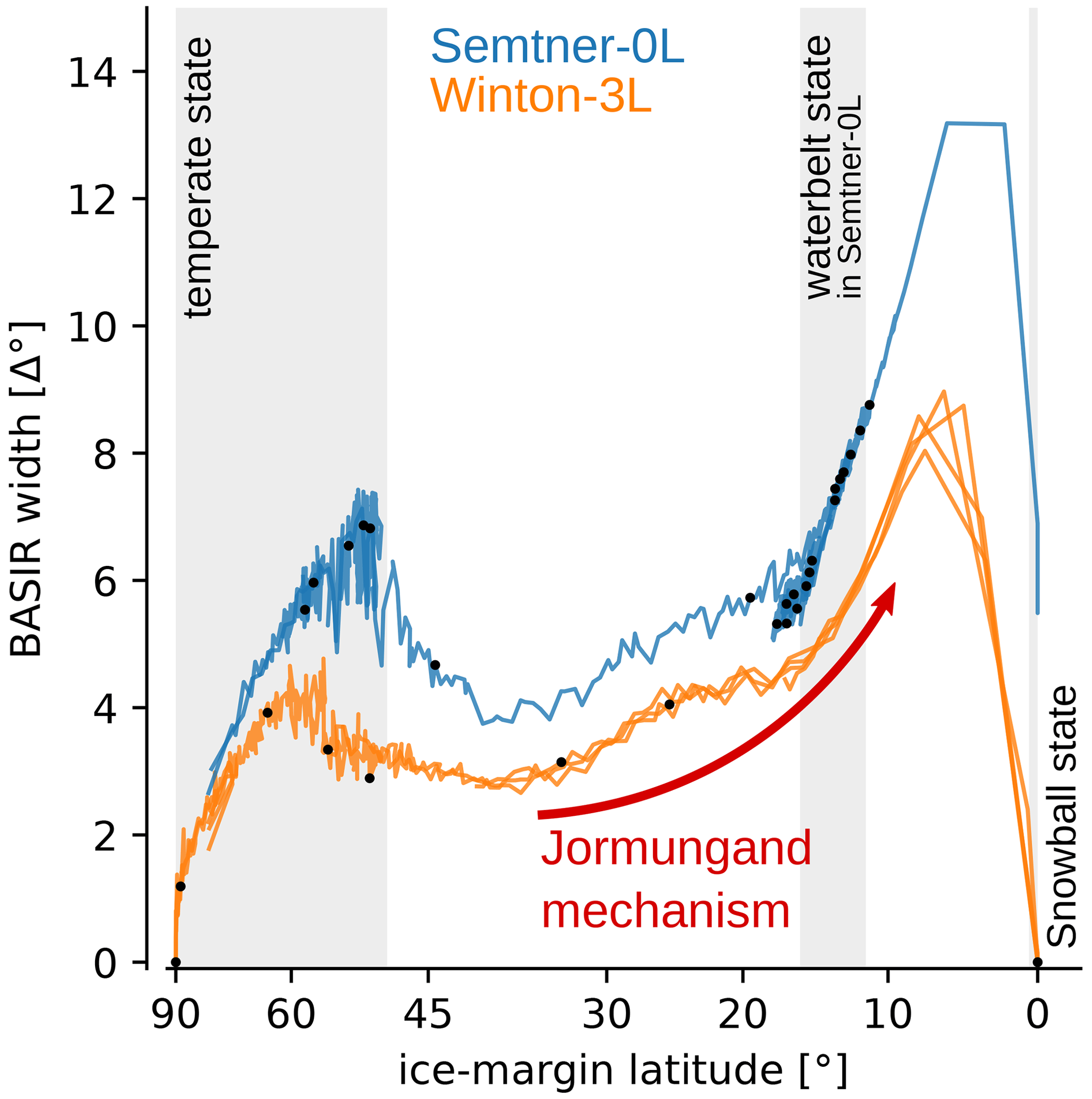
Figure 2 Width of the bare sea-ice region (BASIR) at the ice margin in degree latitude as a function of the transient latitude of the ice margin. For example, for an ice-margin latitude of 10° and a BASIR width of 10°, sea ice extends from the poles to 10° N/S, with bare ice between 10–20° N/S and snow-covered ice between 20 and 90° N/S. Gray boxes indicate the ranges of ice-margin latitudes where stable states are found in Semtner-0L (see Fig. 1b). Black points are plotted every 50 years after the start of each simulation to emphasize the position of stable states with a constant ice-margin latitude.

3.2 Jormungand mechanism

The difference between Semtner-0L and Winton-3L results from a strong difference in snow cover. Figure 2 shows the BASIR width for all simulations as a function of the ice-margin latitude. Independent of CO₂, Semtner-0L results in a wider BASIR than Winton-3L. In Semtner-0L, the BASIR widens with increasing global ice cover and reaches its maximum between 60 and 50°, near the tipping point marking the edge of the attractor of the temperate state. Following this, the BASIR width sharply decreases as sea ice reaches the midlatitudinal precipitation maximum. When sea ice passes 30°, the Jormungand mechanism becomes apparent. The BASIR width increases, as the negative P–E balance in the subtropics results in net snow melt. Ultimately, this results in stable waterbelt states at an ice-margin latitude between 12 and 15°, with a BASIR width of around 6.5°.

In Winton-3L, the BASIR width shows the same general features, but the BASIR is narrower for all sea-ice margins, as there is a larger snow cover on the ice. Although the Jormungand effect leads to a widening of the BASIR when sea ice reaches the subtropics in Winton-3L as well, the effect is much smaller than in Semtner-0L. This is caused by a large difference in surface melting near the ice margin, as can be seen in Fig. 3.

Figure 3a shows the zonal mean P–E balance and its components, as well as surface ablation when the sea-ice margin is at 12° in both models. Surface ablation includes melting and sublimation of both sea ice and snow, with melting being the dominant contribution. The P–E balance and its components, precipitation and evaporation, are almost identical in both models. Surface ablation, on the other hand, is up to twice as large in Semtner-0L as in Winton-3L in the region directly poleward of the sea-ice margin. This is a manifestation of the melt-ratchet effect. The neglected heat capacity in Semtner-0L results in a larger diurnal cycle of surface temperature and consequently larger surface melting. Ultimately, this results in thinner snow cover on ice (Fig. 3b), leading to a smaller BASIR width.

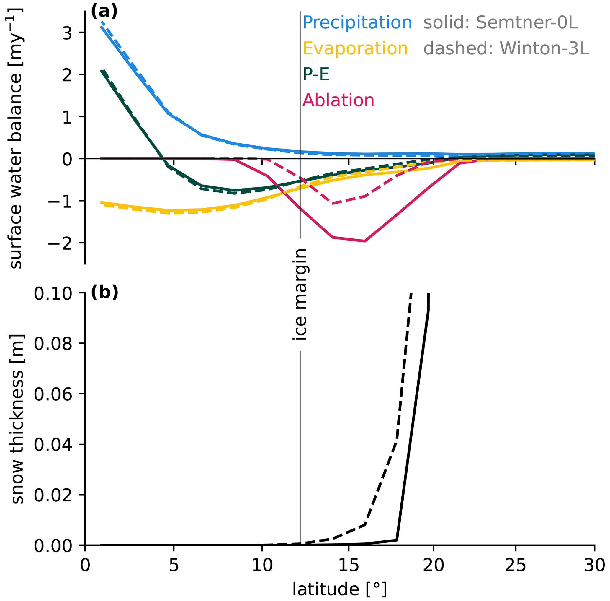
Figure 3 Zonal averages of precipitation, evaporation, precipitation–evaporation, surface ablation of sea ice and snow (a), and snow thickness (b) in simulations using Semtner-0L (solid lines) and Winton-3L (dotted lines). The data are time-averaged over simulations from Semtner-0L and Winton-3L that have a sea-ice margin in the range between 11.25 and 13.125°, corresponding to one bin in Fig. 4. Vertical black lines indicate the center of the bin.

The difference in BASIR width modulates the ice–albedo feedback and hence determines waterbelt stability. To demonstrate this, we analyze the meridional structure of top-of-atmosphere (TOA) albedo as a function of the ice-margin latitude. More specifically, we aggregate data from two transient simulations with Semtner-0L and Winton-3L to cover the range from ice-free to Snowball states. For Semtner-0L, we aggregate the simulations with 5000 and 5500 ppmv CO₂ and for Winton-3L the simulations with 8000 and 8500 ppmv CO₂. Monthly and zonal mean output data of the simulations are binned according to the latitude of the ice margin, and data in each ice-margin latitude bin are averaged over all months in that bin. The result is the meridional distribution of TOA albedo as a function of ice-margin latitude shown in Fig. 4. The number of values per bin varies significantly, depending on how long the ice margin stays in that bin. This is illustrated by the histograms on top of panels (a) and (b) in Fig. 4.

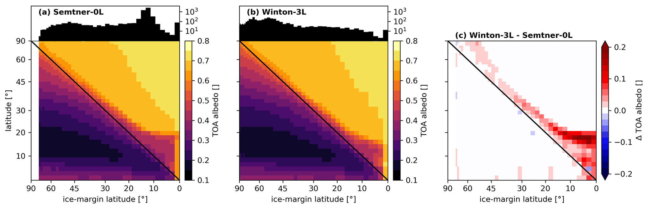
Figure 4 Meridional distribution (y axis) of zonal mean top-of-atmosphere (TOA) albedo (colors) as a function of the transient ice-margin latitude (x axis). The histograms on top of panels (a) and (b) show the number of data points per bin. (a) Semtner-0L. (b) Winton-3L. (c) Difference between Winton-3L and Semtner-0L.

The differences in BASIR width at the ice margin result in different TOA albedos in Semtner-0L compared to Winton-3L (Fig. 4c). The largest difference is located directly poleward of the ice margin. The albedo difference around the ice margin increases strongly as soon as the ice margin moves equatorward of 30°. This indicates the larger BASIR widening and thus stronger Jormungand mechanism in Semtner-0L. Importantly, strong differences in the TOA albedo occur for subtropical sea ice equatorward of 20°. This is because subtropical sea ice is bare in Semtner-0L as demanded by the Jormungand mechanism, but some snow is in fact able to persist on top of subtropical sea ice in Winton-3L. Consequently, waterbelt states are found in Semtner-0L with stable ice margins between 15 and 20°, and no waterbelt states are found in Winton-3L.

3.3 TOA energy budget

The widening of the BASIR when ice enters the subtropics lowers the TOA albedo and leads to a weakening of the ice–albedo feedback. In Semtner-0L, but not in Winton-3L, the weakening is strong enough to bring the TOA energy budget into equilibrium for waterbelt states. This behavior is illustrated in Fig. 5, which shows the global mean TOA energy budget in panel (a) and its shortwave and longwave components in panels (b) and (c).

Both ice models start out with a TOA energy budget close to equilibrium for ice margins corresponding to temperate climate states. When ice advances equatorward of 50°, the energy budget becomes more and more negative due to the runaway ice–albedo feedback. For Semtner-0L, the Jormungand mechanism becomes evident as the TOA energy budget reaches a local minimum for an ice margin of 30° and subsequently increases again until equilibrium is reached in a waterbelt state. Instead, for Winton-3L the TOA energy budget only shows a slight slowdown, and the Jormungand mechanism is not strong enough to restore the TOA energy budget into equilibrium.

The longwave component of the TOA energy budget depicted in Fig. 5c is mostly determined by temperature and the Planck feedback and is hence essentially the same in Semtner-0L and Winton-3L. Small differences are due to the different atmospheric CO₂ content in the simulations. For temperate states, Winton-3L emits marginally less longwave radiation compared to Semtner-0L since a larger CO₂ content is used in the Winton-3L simulations. In the region of the Jormungand state, Semtner-0L and Winton-3L have similar values of atmospheric CO₂ (see Fig. 1b) and hence a very similar longwave radiative flux.

The diverging evolution of the TOA energy budget between Semtner-0L and Winton-3L is driven by the shortwave component, i.e., the ice albedo. The global mean of the absorbed shortwave radiative flux as a function of ice-margin latitude is depicted in Fig. 5b. The slope of this line measures the strength of the ice–albedo feedback. The amount of absorbed shortwave radiation slowly diverges between the two ice models as sea ice expands from the midlatitudes into the subtropics, with Semtner-0L absorbing more shortwave radiation. This is a consequence of the increasing difference in surface albedo due to the difference in BASIR width shown in Fig. 4. In the waterbelt state, the difference is up to 2.5 W m⁻² and increases further for ice margins closer to the Equator as the difference in the BASIR increases. The difference between Semtner-0L and Winton-3L is not driven by clouds, as the clear-sky energy budget exhibits the same behavior (not shown).

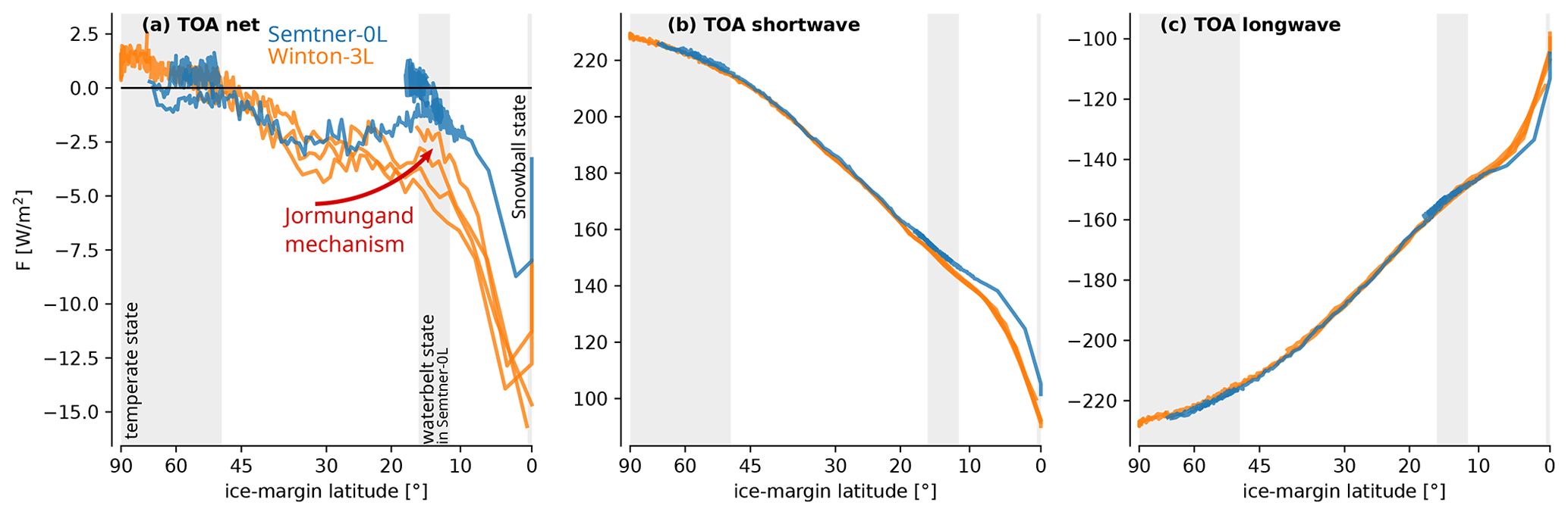
Figure 5 Components of the global mean top-of-atmosphere (TOA) energy budget as a function of the transient ice-margin latitude for all simulations with Semtner-0L (blue) and Winton-3L (orange). (a) Net energy budget. (b) Absorbed shortwave radiation. (c) Outgoing longwave radiation. Fluxes are defined as positive downward for all components. Gray boxes indicate the regions where stable states were found. Note that the TOA net energy balance in the Snowball state is not zero because the simulations were stopped as soon as global ice cover was reached. The TOA net energy balance at this point is not yet in equilibrium.

In summary, the larger surface melting in Semtner-0L due to the stronger melt-ratchet effect results in less snow on the ice and a wider BASIR. This weakens the ice–albedo feedback and strengthens the Jormungand mechanism by decreasing surface and TOA albedo near the sea-ice margin. Consequently, in Semtner-0L the TOA energy budget can be in equilibrium for low-latitude sea-ice margins, and waterbelt states are possible, whereas Winton-3L falls into a Snowball state.

3.4 Effect of ice model on snow cover

To further illustrate that Winton-3L favors more snow on ice, we perform an additional simulation with Winton-3L that is restarted from a stable waterbelt state simulated with Semtner-0L. The Winton-3L simulation is branched off from year 400 of the Semtner-0L simulation with 8000 ppmv CO₂ at year 400 (see Fig. 1). The initial internal ice temperatures that are required for the Winton-3L model are obtained from the ice surface temperatures from the restart file of the Semtner-0L simulation.

The 3L-Winton simulation falls into a Snowball state after 6 years. This is shown in terms of surface albedo in Fig. 6. The lower part of the figure depicts the first year in higher temporal resolution and the upper part the subsequent years until global glaciation is achieved. In Winton-3L surface albedo increases quickly within the first few months in the region of ice that is bare in Semtner-0L. This indicates that snow quickly accumulates on ice in Winton-3L and that the BASIR narrows. After 6 months the border between snow-free and snow-covered ice has clearly shifted towards the Equator in Winton-3L (dotted lines), and the increase in surface albedo has led to global cooling and more ice growth also in the summer (northern) hemisphere. In the following months and years until glaciation, this poses a feedback loop of increased snow cover in both summer and winter hemispheres, larger ice cover in the summer hemisphere, higher surface albedo, and lower temperatures.

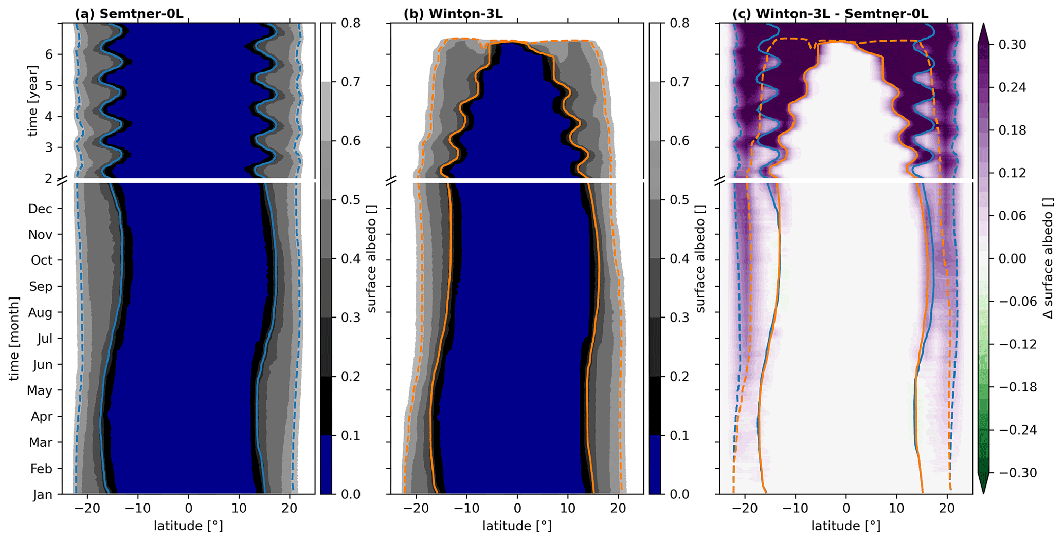
Figure 6 Zonal mean surface albedo for Semtner-0L (a) and Winton-3L (b) simulations as a function of time. The Winton-3L simulation is restarted from the stable Semtner-0L waterbelt simulation. Both simulations use 8000 ppmv CO₂. Solid lines indicate the ice margin, and dashed lines indicate the snow margin. (c) Difference in surface albedo between the Winton-3L and Semtner-0L simulations, with the ice and snow margin lines of both simulations overlaid. The initial year is shown with an enlarged time axis, and the following 5 years is depicted with a squeezed time axis.

4 Conclusions

Previous work proposed that waterbelt states with low-latitude ice margins are possible thanks to the Jormungand mechanism. The Jormungand mechanism is based on a widening of the region of bare sea ice (abbreviated as BASIR) near the sea-ice margin when sea ice enters the subtropics, which decreases subtropical ice albedo and can stop the runaway ice–albedo feedback and stabilize the ice margin at around 15° (Abbot et al., 2011). In this study, we investigate the robustness of such waterbelt states with respect to the representation of the thermodynamics of sea ice. To this end, we conduct simulations with the ICON-A atmosphere model in an idealized aquaplanet setup using the simple zero-layer Semtner sea-ice model and the more sophisticated energy-conserving three-layer Winton model.

The main finding of our work is that stable waterbelt states are possible and accessible in the zero-layer Semtner model but not in the three-layer Winton model. We show that the lack of waterbelt states in the three-layer Winton model results from a narrower BASIR, which weakens the Jormungand mechanism and strengthens the ice–albedo feedback compared to the simulations with the zero-layer Semtner model. The BASIR is narrower in the three-layer Winton model because taking into account the vertical resolution and ice heat capacity decreases surface melting and allows more snow to accumulate on top of sea ice, in particular in the subtropics.

That ice vertical resolution is important to correctly simulate surface melting and hence Snowball Earth climates has been shown before by Abbot et al. (2010), Yang et al. (2012a, b) and Hörner et al. (2022), who demonstrated that insufficient vertical resolution overestimates surface melting due to a melt-ratchet effect. In Hörner et al. (2022) we specifically showed that insufficient vertical resolution enhances Snowball Earth initiation by allowing more ice and snow to persist into the summer months. Here, we study the effect of ice vertical resolution on the ice–albedo feedback over a wider range of climate states and find that the impact of vertical resolution becomes increasingly important as the ice margin moves toward the Equator. As a result, the vertical resolution of sea ice can determine the existence and stability of a waterbelt state by controlling the width of the BASIR.

Our results question the validity of waterbelt states. However, previous studies with a range of different sea ice models found waterbelt states. So, how important is the Jormungand mechanism, and how does it compare to other mechanisms? We briefly discuss this question in the following and note that, although the Jormungand mechanism may not be able to stabilize a waterbelt state on its own, it might add to other stabilizing mechanisms so that a waterbelt state might be possible.

• Multiple studies found waterbelt states in the atmospheric model CAM and the Earth system model family CCSM/CESM that CAM is part of (Abbot et al., 2011; Yang et al., 2012a, b; Wolf et al., 2017; Braun et al., 2022). These studies used a five-layer sea-ice scheme, which, based on our results, should lead to an even narrower BASIR and weaker Jormungand mechanism than in our three-layer Winton simulations. Braun et al. (2022) argued that optically thick mixed-phased clouds in the subtropics are in fact needed to stabilize the waterbelt state by muting the ice–albedo feedback in the CAM-idealized aquaplanet simulations of Abbot et al. (2011). On the other hand, it seems likely that the stable waterbelt states simulated in the coupled simulations of Yang et al. (2012a) and Yang et al. (2012b) are possible thanks to heat convergence near the ice margin by the ocean circulation.

• Continental configuration and surface topography might influence the stability of waterbelt states through snow cover on land. For example, Liu et al. (2018) showed with CESM that snow cover on land can decrease as the climate cools when surface topography blocks the moisture import from oceans onto the continental interiors. This could provide a stabilizing feedback that works in favor of waterbelt states.

• The Massachusetts Institute of Technology General Circulation Model (MITgcm) (e.g., Marshall et al., 2004) allows for waterbelt states that are solely stabilized by ocean heat transport (e.g., Rose, 2015; Brunetti et al., 2019; Ragon et al., 2022; Zhu and Rose, 2022). MITgcm uses the same thermodynamic three-layer Winton sea-ice model as our study. The waterbelt state in these studies does not show any BASIR. According to Rose (2015), this is because the ice margin is located further poleward, between 21 and 30° latitude. This is outside the influence of the descending branch of the Hadley cell and thus outside the influence of the Jormungand mechanism. As they are stabilized by different mechanisms, they can be considered different climate states. This demonstrates that both mechanisms can stabilize a waterbelt state on their own.

• The atmosphere model ECHAM5 was used by Abbot et al. (2011) to first demonstrate the Jormungand mechanism in an idealized aquaplanet simulation, and its coupled atmosphere–ocean version ECHAM5-MPIOM was used by Voigt and Abbot (2012) to test the robustness with respect to sea-ice dynamics. Both ECHAM5 and ECHAM5-MPIOM used a zero-layer Semtner model. ECHAM5 did not track snow on the ice, and, because of this, the BASIR had to be hard-coded into the model. The ECHAM5-MPIOM simulations showed that, while the Jormungand mechanism appeared to be active, it was not strong enough to allow for waterbelt states that are separated from temperate states by a bifurcation, and the strong sea ice dynamics in the model inhibited stable subtropical ice margins.

• The ICON model is the successor of ECHAM5 and ECHM5-MPIOM and also uses the zero-layer Semtner sea-ice scheme in its standard version. Braun et al. (2022) demonstrated that the ICON model has difficulties in simulating stable waterbelt states because subtropical clouds are not reflective enough in the model. If cloud optical thickness and cloud reflectivity are increased, the Jormungand mechanism leads to waterbelt states in ICON.

Our results show that, in order for the Jormungand mechanism to lead to stable waterbelt states, the region of bare sea ice needs to be sufficiently wide. Simulations with simplified sea-ice models overestimate the width of the bare sea-ice region and therefore likely overestimate the stability of waterbelt states. Consequently, waterbelt states that rely exclusively on the Jormungand mechanism might only be possible for rather peculiar combinations of a coarse vertical resolution of ice and optically thick subtropical clouds. This suggests that the Jormungand mechanism itself might be secondary and robust waterbelt states are only possible if other stabilizing mechanisms, particularly those from ocean heat transport, are also active.