Carbon fluxes in spring wheat agroecosystem in India

Carbon fluxes from agroecosystems contribute to the variability of the carbon cycle and atmospheric [CO₂]. This study is a follow-up to Gahlot et al. (2020), which used the Integrated Science Assessment Model (ISAM) to examine spring wheat production and its drivers. In this study, we look at the carbon fluxes and their drivers. ISAM was calibrated and validated against the crop phenology at the IARI wheat experimental site in Gahlot et al. (2020). We extended the validation of the model on a regional scale by comparing modeled leaf area index (LAI) and yield against site-scale observations and regional datasets. Later, ISAM-simulated carbon fluxes were validated against an experimental spring wheat site at IARI for the growing season of 2013–2014. Additionally, we compared with the published carbon flux data and found that ISAM captures the seasonality well. Following that, regional-scale runs were performed. The results revealed that fluxes vary significantly across regions, primarily owing to differences in planting dates. During the study period, all fluxes showed statistically significant increasing trends (p<0.1). Gross primary production (GPP), net primary production (NPP), autotrophic respiration (R_a), and heterotrophic respiration (R_h) increased at 1.272, 0.945, 0.579, 0.328, and 0.366 TgC yr⁻², respectively. Numerical experiments were conducted to investigate how natural forcings such as changing temperature and [CO₂] levels as well as agricultural management practices such as nitrogen fertilization and water availability could contribute to the rising trends. The experiments revealed that increasing [CO₂], nitrogen fertilization, and irrigation water contributed to increased carbon fluxes, with nitrogen fertilization having the most significant effect.

1 Introduction

Croplands are highly productive ecosystems that exchange energy, carbon, and water with the atmosphere (Lokupitiya et al., 2016). Croplands absorb a significant amount of carbon from the atmosphere during their short growing season, contributing to seasonal variations in atmospheric carbon loading. The rise in carbon levels in the atmosphere has complicated effects on agricultural productivity (Yoshimoto et al., 2005; Saha et al., 2020). Temperature, nitrogen fertilizers, and irrigation are all factors that influence crop development and, as a result, alter carbon fluxes from croplands (Lin et al., 2021). For example, increasing temperature can offset the beneficial effects of increased atmospheric carbon (Sonkar et al., 2019). Better-fertilized soil can respond better to higher carbon levels (Lin et al., 2021). Lands with limited water availability have lower carbon fluxes (Hatfield and Prueger, 2015; Green et al., 2019). Understanding the variability and drivers of carbon fluxes from agroecosystems can thus contribute to a better understanding of the interactions between the biosphere and the atmosphere.

Wheat is one of the world's most widely farmed cereal crops and a staple food for approximately 2.5 billion people (Ramadas et al., 2020). Winter wheat and spring wheat are the two cultural types of wheat grown worldwide. Spring wheat is grown in India. Spring wheat is typically planted in October–November and harvested between March and April in India (Ramadas et al., 2020). With approximately 107 Mt in 2020, India ranks second only to China in wheat production, accounting for 13.5 % of the global wheat supply (FAOSTAT, 2019). Wheat production in India has increased by 25 % since 2008. The harvested area increased from 28 Mha in 2008 to 29 Mha in 2019 (FAOSTAT, 2019). However, research into carbon in spring wheat croplands is limited. The current study is the first to evaluate the carbon dynamics and the impact of their drivers in the Indian agroecosystem.

Baldocchi et al. (2018) extensively reviewed the variability of carbon fluxes from terrestrial ecosystems across the globe, but there are no studies from the Indian subcontinent. A few studies examined carbon fluxes at the site scale in northern Indian spring wheat agroecosystems. Patel et al. (2011) for the 2008–2009 growing season, Patel et al. (2021) for the 2014–2015 growing season, and Kumar et al. (2021) for the 2013–2014 growing season are examples of these studies. All studies found the typical U-shaped curve in the net ecosystem production (NEP) at diurnal and seasonal scales. The average NEP during the growing season was 5–6 gC m⁻² d⁻¹. Only the intra-annual variation of carbon fluxes can be discussed in site-scale studies. Studying interannual variability in carbon fluxes is difficult because flux towers are only operational for 1 or 2 years. Furthermore, there are only a few flux towers in the agroecosystems of India, and they are all installed in the northern region. Site-scale carbon studies cannot be extended to understand carbon fluxes at a regional scale over India because the climate and growing conditions vary considerably across wheat-growing regions of India.

Process-based models are commonly used to study carbon dynamics (Sándor et al., 2020). These models explicitly characterize known or hypothesized cause-and-effect relationships between physiological processes and environmental driving forces (Chuine and Régnière, 2017). Process-based crop models can simulate crop production, phenology, carbon, energy fluxes, and the interannual variability in crop carbon budgets using atmospheric and management data as inputs (Revill et al., 2019). This study used the Integrated Science Assessment Model (ISAM), a process-based land surface model with bio-geochemical and bio-geophysical components. ISAM was developed to assess the effect of variations in CO₂ concentration on agroecosystems (Jain and Yang, 2005; Song et al., 2013; Yang et al., 2009).

The main benefit of using process-based models is that they can quantify the direct effect of input parameters and external drivers on crop growth and fluxes (Jones et al., 2017). There are a few studies on carbon fluxes in Indian terrestrial ecosystems (Banger et al., 2015; Gahlot et al., 2017), but none on agroecosystems. A significant bottleneck in modeling agroecosystems in India is the lack of observation data on crop phenology. We are trying to bridge the gap between the on-field research extensively carried out across India at agricultural institutions and modeling studies through our efforts to digitize the research into a machine-readable format. As a result, we assembled comprehensive crop phenology data for spring wheat for the first time. These efforts will be extended to a variety of crops grown across India.

To our knowledge, no long-term regional-scale studies of carbon dynamics over Indian agroecosystems have been conducted. Crop management practices can significantly impact crop growth and interaction with the land and atmosphere via water, energy, nutrients, and carbon exchanges. There has been no research on the impact of these management practices on carbon fluxes in Indian agroecosystems. The current study is the first to address these issues, significantly contributing to our understanding of terrestrial carbon dynamics using a land surface model.

The overarching goal of this study is to investigate carbon dynamics over spring wheat croplands in India and quantify the role of various natural and anthropogenic drivers that govern carbon fluxes. The specific goals of this paper are (i) to validate the ISAM simulation of Indian spring wheat, (ii) to investigate the spatiotemporal variation in carbon fluxes over spring wheat croplands in India, and (iii) to quantify the effect of external drivers such as changing temperature and [CO₂] as well as agricultural management practices.

2 Methodology

2.1 Modeling approach

ISAM has a dynamic growth module to simulate various crops (Song et al., 2013). Gahlot et al. (2020) used the dynamic crop module to represent Indian spring wheat by calibrating the allocation and growth parameters (supplement of Gahlot et al., 2020). The allocation and the growth parameters were calibrated using data from the experimental site at IARI, New Delhi, which was operational for three growing seasons: 2013–2014, 2014–2015, and 2015–2016. Carbon fluxes were measured during the 2013–2014 growing season, and phenology data were measured during the latter two seasons. ISAM was calibrated and validated using phenology observations from the 2014–2015 and 2015–2016 growing seasons (Gahlot et al., 2020). Taking this work forward, we used the same configuration of the model to estimate the carbon fluxes in the spring wheat croplands of India. The modeling approach used in the study is as follows. First, ISAM was run in site-scale mode to simulate the carbon fluxes at the IARI site driven by prescribed management data. The simulations were evaluated against field measurements from the IARI site for the 2013–2014 growing season. Next, ISAM was run at a country scale to simulate carbon fluxes over wheat-growing regions of India from 1901–2016. Finally, we conducted numerical experiments to simulate the impacts of environmental drivers and agricultural management practices on carbon fluxes.

2.2 Model description

This study used ISAM in the same configuration as Gahlot et al. (2020). For brevity, here we briefly describe the model and its configuration. More details are available in Gahlot et al. (2020) and Gahlot (2020). We used two versions of ISAM crop modules to validate the improvements made by Gahlot et al. (2020), ISAM${}_{{\mathrm{C}}_{\mathrm{3}}\mathrm{\_}\mathrm{crop}}$ and ISAM_{dyn_wheat}. The two versions were run for the same period and used the same input data, and the simulated carbon fluxes were compared. The ISAM${}_{{\mathrm{C}}_{\mathrm{3}}\mathrm{\_}\mathrm{crop}}$ module has static phenology and prescribed leaf area index (LAI) using observations from the Moderate Resolution Imaging Spectroradiometer (MODIS) aboard the Terra and Aqua satellites. The ISAM${}_{{\mathrm{C}}_{\mathrm{3}}\mathrm{\_}\mathrm{crop}}$ module used a static root parameterization with fixed rooting depth and fixed root fraction in each soil layer. Energy and water fluxes as well as carbon assimilation are calculated through coupled canopy photosynthesis, energy, and hydrological processes. Assimilated carbon is allocated to vegetation pools in fixed fractions. Gahlot et al. (2020) used the dynamic equations in ISAM developed by Song et al. (2013) for soybeans and updated a few parameters from the literature and a few through calibration to simulate spring wheat (ISAM_{dyn_wheat}) (supplement of Gahlot et al., 2020). ISAM_{dyn_wheat} differs from the static version in three schemes: dynamic phenology, carbon allotment, and vegetation structure growth. For example, allocating net assimilated carbon to leaves, roots, stems, and grain pools at each model time step is a dynamic process based on the crop's light, temperature, water, and nitrogen availability. This allocation scheme aims to minimize the adverse effects of limited light, water, and nutrient stress on the crop (Gahlot, 2020). For more details on the dynamic modules in ISAM_{dyn_wheat}, please refer to Gahlot (2020).

ISAM_{dyn_wheat} is equipped with dynamic planting date criteria and heat stress modules to simulate the effects of environmental factors on the spring wheat growing season and phenology (Gahlot et al., 2020). The dynamic planting date is calculated in ISAM, as shown in Table S2 of Gahlot et al. (2020). The wheat-growing regions are divided based on the 1901–1950 climatological minimum temperature. A specific criterion is assumed for each region depending on the region's characteristics (Table S2: Gahlot et al., 2020).

Yield is a proxy for the carbon uptake by the crops. The initial reproductive stage in ISAM marks the onset of the storage organs. The allocation of assimilated carbon to the storage organ begins, and the vegetative development of the plant stops. The next stage, the post-reproductive stage, marks the solidification of grains and increased nutrient allocation to the grains while ensuring that capable roots support the plant. After the crop reaches maturity, the total grain allocation from the initial reproductive stage to maturity is converted to yield. Various factors like light availability, temperature stress, and nitrogen availability act as limiting factors to crop growth, and nutrient allocation is promoted in the crop so that the impact of these factors is minimized (supplement of Gahlot et al., 2020). Since yield is a major part of the carbon taken up by the crop, its validation against observations is necessary and is shown in Sect. 3.2.

ISAM simulates the processes through which external drivers can affect crop growth. For example, temperature influences maximum carboxylation rates, which regulates carbon assimilation (Song et al., 2013). ISAM can simulate nitrogen dynamics and the interactive effects of carbon–nitrogen cycles caused by climate change or increasing [CO₂] (Yang et al., 2009). Nitrogen fertilization through deposition onto the soil serves as a nitrogen input to the ISAM nitrogen cycle (Jain et al., 2009). When water and mineral N are scarce, the carbon cycle and assimilation suffer because of reduced carbon allocation to leaves and stems (Song et al., 2013). Added water through irrigation reduces the water stress on crops in water-limited situations, thereby increasing carbohydrate production.

2.3 Data for model evaluation

To evaluate the ISAM_{dyn_wheat} crop phenology and yield, we digitized the spring wheat crop dataset from 2000–2021. The dataset was extracted from the theses of MSc and PhD students at various agricultural institutions across India. Until recently, these theses were not available in the public domain, but through the efforts of KRISHIKOSH, a thesis repository, it now holds a large number of theses. The dataset we compiled comprises nine spring wheat sites and 26 growing seasons (Table S1). Comparing the spring wheat phenology and yield simulated by ISAM across 26 growing seasons adds to the much-needed validation of ISAM.

Field observations of carbon fluxes are limited in India, and none are available in the public domain. We obtained field observations of carbon fluxes for the 2013–2014 spring wheat-growing season from the IARI (New Delhi) experimental spring wheat farm (Kumar et al., 2021). The farm, covering 650 m², is located at 28^∘40^′ N, 77^∘12^′ E. The site has an eddy covariance (EC) flux tower that gave gross primary production (GPP), total ecosystem respiration (TER), and net ecosystem production (NEP). The tower had enough area to ensure an upwind stretch of homogeneous vegetation, essential for measuring fluxes using the EC technique (Schmid, 1994). The spring wheat crop was planted on 16 December 2013 at the site. Nitrogen fertilizer at 120 kg N ha⁻¹ was applied in three installments of 60, 30, and 30 kg N ha⁻¹ on the planting day and the 25th and 67th days after sowing. The field was irrigated five times throughout the growing season to avert water stress.

To extend our validation of carbon fluxes simulated by ISAM, we conducted a literature review to find papers that reported carbon fluxes from spring wheat. We found two such studies: Patel et al. (2011) and Patel et al. (2021). Data were not available as a supplement in these papers. Therefore, we extracted the data from the figures. We extracted the monthly mean NEP data from Fig. 2 of Patel et al. (2011) and Fig. 2b of Patel et al. (2021). Although we extracted the flux data, we do not have the field activities to simulate site-scale simulations. Therefore, we compared our regional-scale simulations against these carbon flux data.

2.4 Meteorological and management data

All ISAM simulations need data for both environmental and anthropogenic drivers. We used annual atmospheric [CO₂] data from Le Quéré et al. (2018) and climate data from Viovy (2018) for both site-scale and country-scale simulations. The temporal resolution of the climate data is 6 h, and we interpolated the climate data to hourly values. The planting date, nitrogen, and irrigation data used for the site-scale runs are described in Sect. 2.3.

For the country-scale runs, we used nitrogen fertilizer data developed by Gahlot et al. (2020) by combining data from Ren et al. (2018) and Mueller et al. (2012). Data on the harvested wheat area in a gridded format are needed (1980–2016) for calculating fluxes at a country scale in units of teragrams of carbon per year (TgC yr⁻¹). We used spring wheat harvested area data developed by Gahlot et al. (2020), combining harvested area from Monfreda et al. (2008) and MAFW (2017).

2.5 Experimental design

2.5.1 Site-scale simulations at the IARI site

Gahlot et al. (2020) calibrated and validated ISAM using phenology observations from the 2014–2015 and 2015–2016 growing seasons. We designed a site-scale carbon flux experiment to validate ISAM carbon fluxes against field observations for the growing season of 2013–2014. To simulate the carbon fluxes at a site scale, ISAM was spun up for the 2013–2014 growing season using climate data from Viovy (2018), annual atmospheric [CO₂] data from Le Quéré et al. (2018), and airborne nitrogen deposition data (Dentener, 2006) until the soil parameters reached a steady state. The steady-state conditions used in the study are the same as those followed by Yang et al. (2005). Further details on the site-scale spin-up are available in Gahlot et al. (2020).

We used ISAM_{dyn_wheat} in the same configuration as Gahlot et al. (2020) to simulate carbon fluxes for the 2013–2014 growing season.

2.5.2 Country-wide simulations over wheat-growing regions of India

The country-wide simulations were designed to understand the spatial variation of carbon fluxes across India's wheat-growing regions using the ISAM_{dyn_wheat} module. To simulate the carbon fluxes at a regional scale, ISAM was spun up for 1901 to maintain constant soil parameters such as temperature, moisture, and carbon and nitrogen pools. For the spin-up, we used the climate data from Viovy (2018) for the years 1901–1920, with airborne nitrogen deposition (Dentener 2006) and [CO₂] (Quéré et al., 2018) held at levels of 1901 and neglecting nitrogen fertilizer and irrigation.

We used ISAM_{dyn_wheat} to conduct regional-scale simulations over wheat-growing regions of India to understand the variability of carbon fluxes across diverse climates (Ortiz et al., 2008) and management conditions. We ran the model for the period 1901–2016. First, we conducted a control run (S_CON) driven by the annual [CO₂], climate data, nitrogen fertilizer data, and full irrigation to meet crop water needs. Irrigation is a crucial factor in spring wheat cultivation, with 93.6 % of the wheat area equipped for irrigation (MOA 2016), and the Indo-Gangetic Plain significantly contributes to the total wheat area irrigated in India (Gahlot et al., 2020). Data on the exact volume of irrigation water were not available. Therefore, in the S_CON simulation, each grid cell was considered 100 % irrigated (i.e., to field capacity), so there was no water stress on the crops (Gahlot et al., 2020).

Our analysis focused on the years 1980–2016. We analyzed country-scale model results as inter-decadal changes from the 1980s to the 2010s. We calculated decadal averages for various fluxes by dividing the total period into the 1980s (1980–1989), 1990s (1990– 1999), 2000s (2000–2009), and 2010s (2010–2016). The regional-scale simulations validate the crop phenology and yield of spring wheat. The crop dataset we compiled was compared with the 26 growing seasons of data.

Figure 1 Comparison of observations and ISAM fluxes for (a) GPP, (b) TER, and (c) NEP.

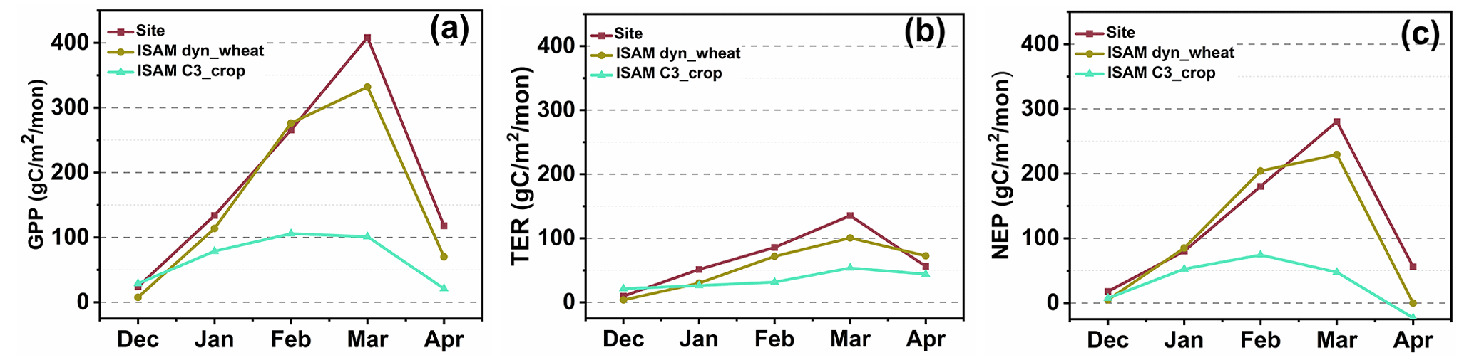
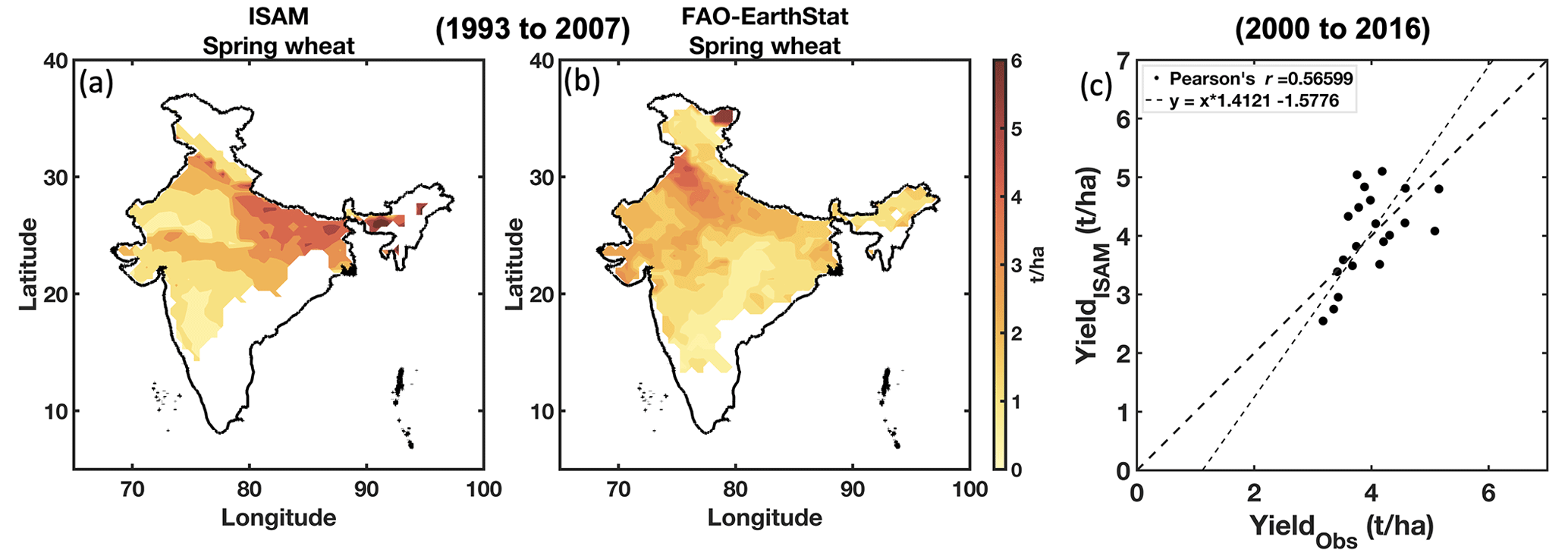
Figure 2 Comparison of (a) yield simulated by ISAM and (b) EarthStat gridded data. (c) Yield simulated by ISAM against yield observations from the spring wheat crop dataset.

2.5.3 Experiments to estimate the effect of external drivers on carbon fluxes

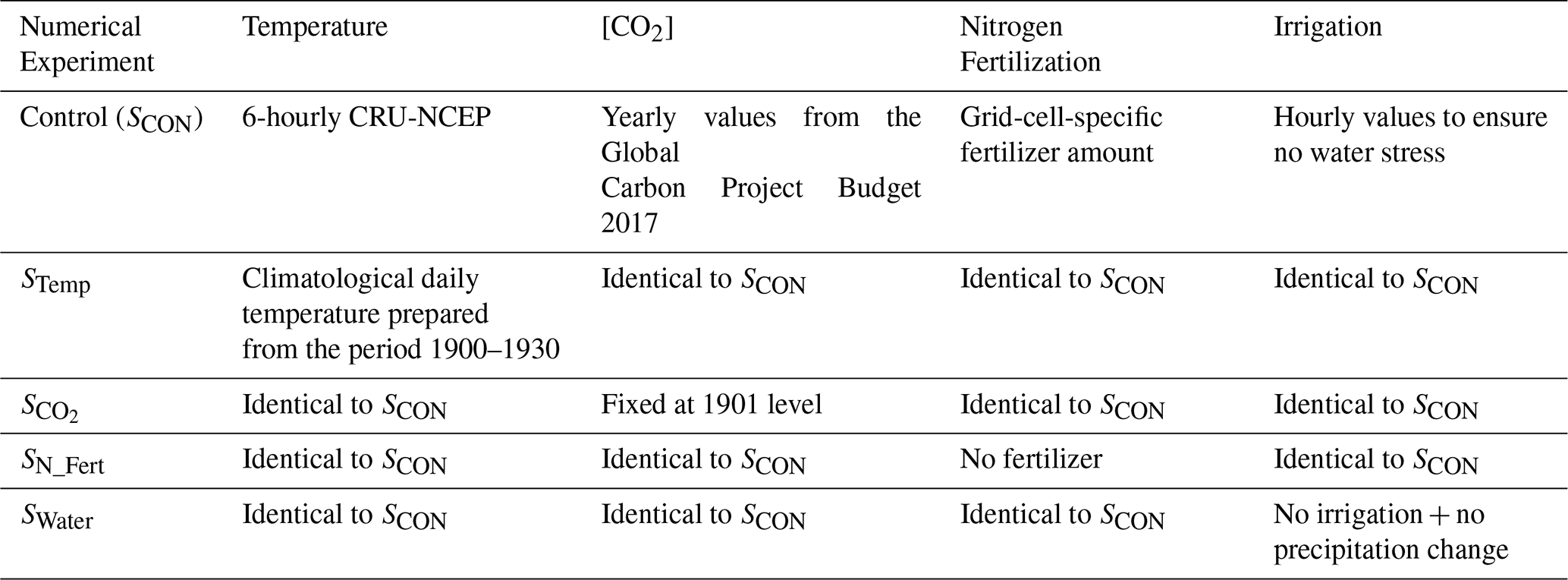
Environmental drivers like temperature and [CO₂] as well as agricultural management practices like applying nitrogen fertilizers and irrigation influence spring wheat growth and are likely to influence carbon fluxes. We conducted four additional experimental simulations to quantitatively estimate these forcings' effects. The details of the experiments are given in Table 1. In the control run (S_CON), the model was driven by inputs based on observations that vary over time. In the experimental simulations, the value of an input driver was kept constant during the study period, while others were allowed to vary, as in the S_CON simulation. For example, in S_Temp, the input data for [CO₂], nitrogen, and irrigation were identical to those in S_CON, except for temperature, for which we used the de-trended 1900–1930 climatology. In the S_{N_Fert} case, the [CO₂], temperature, and irrigation were identical to those in S_CON, and nitrogen fertilization was absent. The S_Water case is like S_CON, the only difference being that precipitation climatology was used, and no additional water was provided to the soil through irrigation. We calculated the effect of the individual driver as the difference between the S_CON run and the numerical experiments.

Table 1 Numerical experiments were conducted to evaluate the effect of external drivers on carbon fluxes using ISAM dynamic wheat crops for 1901–2016.

3 Results

3.1 Evaluation of ISAM site-scale simulations

Site-scale ISAM_{dyn_wheat} simulations are validated against observations for the 2013–2014 growing season. Our results show that the spring wheat module ISAM_{dyn_wheat} simulates the magnitude and seasonality of carbon fluxes in spring wheat croplands better than ISAM${}_{{\mathrm{C}}_{\mathrm{3}}\mathrm{\_}\mathrm{crop}}$. Figure 1 and Table 2 compare ISAM_{dyn_wheat} and ISAM${}_{{\mathrm{C}}_{\mathrm{3}}\mathrm{\_}\mathrm{crop}}$ against site observations for monthly average fluxes for the 2013–2014 growing season. Figure 1 shows that the observed carbon fluxes increased from leaf emergence in mid-December 2013. The fluxes increased until they reached their peaks in March, after which they declined until the harvest in April.

The simulated fluxes follow the observed pattern. ISAM_{dyn_wheat} was in better agreement with site observations than the ISAM${}_{{\mathrm{C}}_{\mathrm{3}}\mathrm{\_}\mathrm{crop}}$ model. ISAM_{dyn_wheat} captured the seasonality and accumulated GPP, TER, and NEP for the growing season better than the ISAM${}_{{\mathrm{C}}_{\mathrm{3}}\mathrm{\_}\mathrm{crop}}$ model (Table 2). The ISAM_{dyn_wheat} peak coincided with the observations, whereas the fluxes simulated by the ISAM${}_{{\mathrm{C}}_{\mathrm{3}}\mathrm{\_}\mathrm{crop}}$ model peaked about a month earlier. The ISAM_{dyn_wheat} model in ISAM compares better with site measurements for plant biomass at harvest and maximum LAI than the ISAM${}_{{\mathrm{C}}_{\mathrm{3}}\mathrm{\_}\mathrm{crop}}$ model (Table 2).

Table 2 Various crop parameters of ISAMdyn_wheat and ISAMC3_crop against site measurements. We compared field observations at the IARI experimental wheat farm site and ISAM crop varieties (the dynamic crop and C₃ generic crop) for the growing season of 2013–2014.

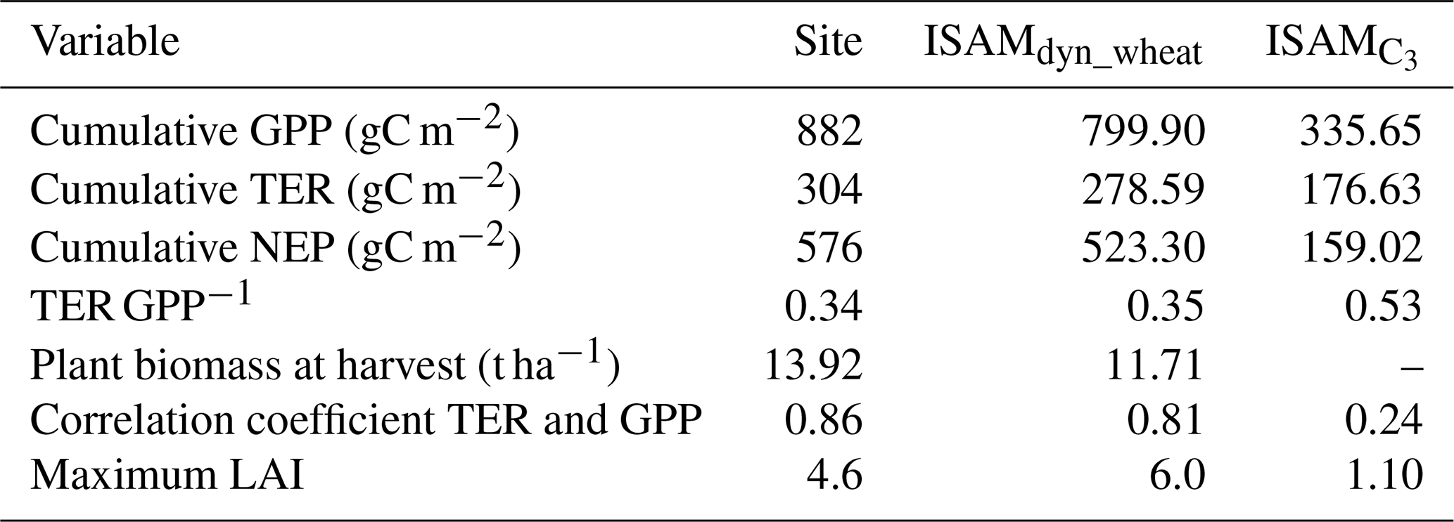
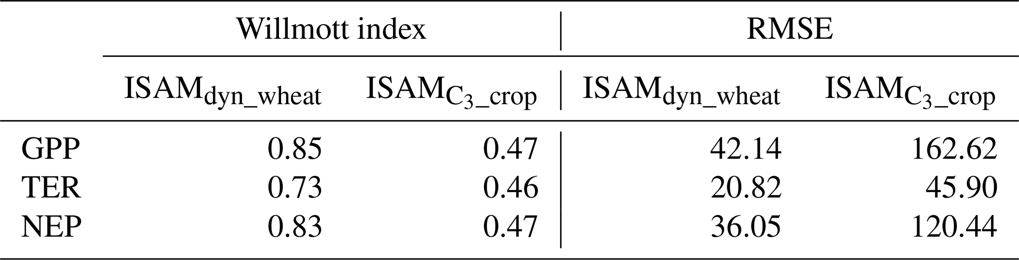
Table 3 shows the Willmott index and RMSE for the two ISAM runs against the site observations. The Willmott index is a more sophisticated tool for evaluating land surface models' efficiency than the usual statistical data comparison indices (Song et al., 2013; Willmott et al., 2012). The Willmott index (Eq. 1) ranges from −1 to 1, where −1 indicates no agreement, while +1 indicates perfect agreement. The Willmott index values for GPP, TER, and NEP for the ISAM_{dyn_wheat} model are 0.85, 0.73, and 0.83, respectively. The corresponding values for the ISAM${}_{{\mathrm{C}}_{\mathrm{3}}\mathrm{\_}\mathrm{crop}}$ model are much lower at 0.47, 0.46, and 0.47, respectively. The higher index value for the dynamic crop suggested better agreement of ISAM_{dyn_wheat} over ISAM${}_{{\mathrm{C}}_{\mathrm{3}}\mathrm{\_}\mathrm{crop}}$ with the site-scale observations.

$$\begin{array}{}\text{(1)}& {\displaystyle }\mathrm{Willmot}\mathrm{index}=\left\{\begin{array}{l}\mathrm{1}-\frac{{\sum }_{i=\mathrm{1}}^n\left|{\mathrm{Model}}_i-{\mathrm{Obs}}_i\right|}{c\cdot {\sum }_{i=\mathrm{1}}^n\left|{\mathrm{Obs}}_i-\stackrel{\mathrm{‾}}{\mathrm{Obs}}\right|},\\ \mathrm{if}{\sum }_{i=\mathrm{1}}^n\left|{\mathrm{Model}}_i-{\mathrm{Obs}}_i\right|\le c\\ \cdot {\sum }_{i=\mathrm{1}}^n\left|{\mathrm{Obs}}_i-\stackrel{\mathrm{‾}}{\mathrm{Obs}}\right|\\ \frac{c\cdot {\sum }_{i=\mathrm{1}}^n\left|{\mathrm{Obs}}_i-\stackrel{\mathrm{‾}}{\mathrm{Obs}}\right|}{{\sum }_{i=\mathrm{1}}^n\left|{\mathrm{Model}}_i-{\mathrm{Obs}}_i\right|}-\mathrm{1},\\ \mathrm{if}{\sum }_{i=\mathrm{1}}^n\left|{\mathrm{Model}}_i-{\mathrm{Obs}}_i\right|>c\\ \cdot {\sum }_{i=\mathrm{1}}^n\left|{\mathrm{Obs}}_i-\stackrel{\mathrm{‾}}{\mathrm{Obs}}\right|\end{array}\right.\text{(2)}& {\displaystyle }\mathrm{RMSE}=\sqrt{{\displaystyle \frac{{\sum }_{i=\mathrm{1}}^n{\left({\mathrm{Model}}_i-{\mathrm{Obs}}_i\right)}^{\mathrm{2}}}{n}}}\end{array}$$

Here, c=2, n is the number of observations, Model_i represents the ISAM-simulated carbon fluxes, and Obs_i represents the site-scale observations.

Therefore, the ISAM_{dyn_wheat} module appropriately represents spring wheat crop dynamics in ISAM. The dynamic phenology, dynamic carbon allotment, and dynamic vegetation structure growth improve crop simulation in a land surface model. However, one should use caution in calibrating and validating the model with sufficient data.

Table 3 Willmott index and RMSE (gC m⁻² month⁻¹) of monthly carbon fluxes (GPP, NEP, and TER).

3.2 Validation of yield simulated by ISAM

A major limitation of Gahlot et al. (2020) was validating ISAM against just one experimental site. To increase the confidence in model simulations, we compared the sowing date (Fig. S1), LAI (Fig. S2), and yield (Fig. 2) simulated by ISAM_{dyn_wheat} against the crop dataset we compiled.

The yield simulated by ISAM is compared against the gridded EarthStat dataset (Monfreda et al., 2008) and site-scale observations (Fig. 2). The EarthStat data are reported as a 5-year mean yield for 1995, 2000, and 2005. The ISAM simulations over a similar period are compared in Fig. 2. The comparison confirms that the ISAM simulation agrees with the EarthStat gridded data in most wheat-growing regions except for small parts of the eastern and northwestern regions. This bias is explained by the difference in the sowing date simulated by ISAM and the GGCMI dataset (Fig. S1). However, analyzing the LAI site-scale comparison (Fig. S2), the growing season simulated by ISAM in the northwestern region (Jobner site) has good agreement with the observations in three growing seasons (2013, 2014, and 2015). This gives us the confidence that the dynamic planting date module in ISAM performs reasonably well. Additionally, even in the site-scale data we have at the IARI site, the spring wheat is sown on 16 December, which aligns with our ISAM simulations for this region. The northeastern and eastern parts of the wheat-growing areas of India are mostly irrigated, have very fertile soil, and have high yields; one of the largest wheat producers in India is in this region. Therefore, we are confident about the yields simulated by ISAM in this region and believe that the EarthStat data used for this yield generation might be biased. This assumption is supported by the site-scale yield comparison in Fig. 2c, which shows that ISAM-simulated yield has good agreement with the observations (Pearson's r=0.57). The yields are high in the western parts of EarthStat data, a semi-arid region with less rain and no irrigation. These regions often have lower yields, and we believe that the EarthStat data are biased in this region.

3.3 Spatial–temporal variability of carbon fluxes from spring wheat agroecosystems in India

The country-scale S_CON run described in Sect. 2.5.2 was designed to provide a quantitative understanding of the spatiotemporal variability of carbon fluxes across the wheat-growing regions of India. Before evaluating the regional-scale ISAM runs, we compared the simulated NEP from the S_CON run with the carbon flux data from Patel et al. (2011, 2021). The monthly averaged carbon flux data were digitized from the figures. Patel et al. (2011) measured the carbon fluxes from January–April 2009 over spring wheat farmland in Meerut in northern India. The measurements provided diurnal variation of net ecosystem exchange (NEE) during four growing stages: tillering, anthesis, post-anthesis, and at maturity. The diurnal data at a growing stage were averaged, and a value representing a monthly NEE was calculated and converted to NEP. Patel et al. (2021) provided daily NEE values for spring wheat farmland in Saharanpur in northern India. The Patel et al. (2021) data were used to generate the monthly average fluxes for the growing season of 2014–2015. The simulated NEP at the grid cells where Meerut and Saharanpur are located is extracted from the S_CON output. Figure 3 represents the comparison of simulated monthly average NEP (NEP_ISAM) and NEP_OBS measured at Meerut (2009) (Patel et al., 2011) and Saharanpur (2014–2015) (Patel et al., 2021). The sowing dates simulated by ISAM are in the second week of December, while the spring wheat is sown in the last week of November in the observation data. Therefore, Fig. 3 shows the season-to-season comparison of the sites and ISAM simulations. The seasonality at Saharanpur is captured very well, although with a small bias. The R² value for the sites is high and significant at p<0.1, showing that the ISAM-simulated NEP captures the variation in observed NEP. The mean absolute bias between observed and simulated NEP at Saharanpur and Meerut is 30.96 and 43.69 gC m⁻² month⁻¹, respectively. The bias may be because we compare site-scale observations with simulated values averaged over the $\mathrm{0.5}{}^{\circ }\times \mathrm{0.5}{}^{\circ }$ (∼ 2500 km²) grid cell area. Nonetheless, the high correlations with site observations point to the ISAM simulations' robustness.

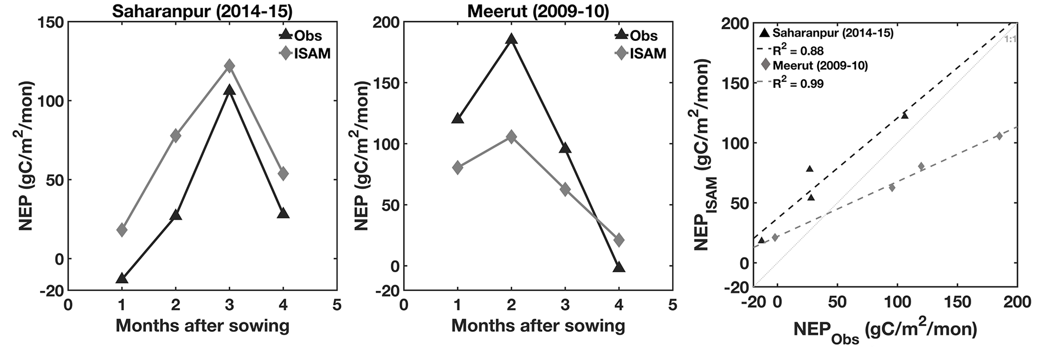
Figure 3 Comparison of the ISAM S_CON with the observations from Saharanpur (Patel et al., 2021) and Meerut (Patel et al., 2011).

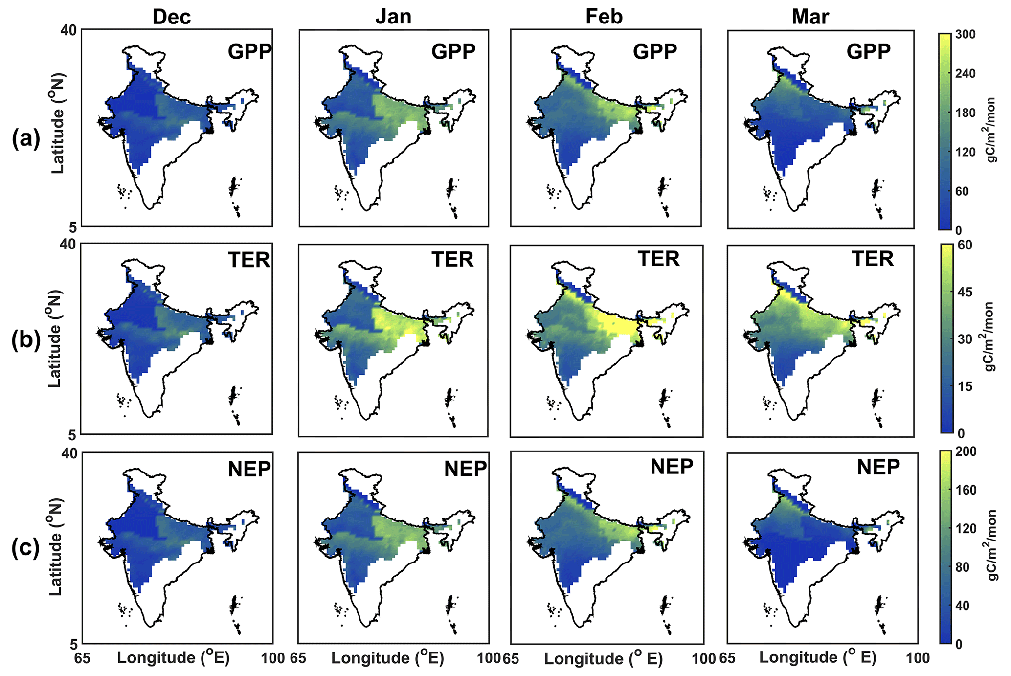
Figure 4 Spatial variation of (a) GPP, (b) TER, and (c) NEP over the wheat-growing regions of India averaged over the period 2000–2016.

Figure 4 shows the spatial maps of GPP, TER, and NEP for the growing season (December–March). The fluxes for each month of the growing season were averaged over 16 years (2000–2016) for that specific month. Because the climatic conditions across wheat-growing regions of India are diverse, the wheat crops are sown on different dates, which was reflected in ISAM using the dynamic planting day criteria. Spring wheat is planted in late October in central India and in early November in eastern India. The northern and northwestern planting dates are late November to early December (Fig. S1). Consequently, there are regional variations in the seasonal flux dynamics. The wheat-growing regions' central and eastern parts show the maximum flux value in January and February, respectively, while the northern and western parts show the maxima in March. The spatial plots show very low values of GPP and NEP during December because the crops are still in early growth. The croplands show very low values of NEP during March in the central and eastern parts of wheat-growing regions. Even though the croplands are not active, heterotrophic respiration leads to moderate values of TER in March for the eastern and central parts of India.

Figure 5 depicts the temporal pattern of annual and decadal fluxes. From 1980–2016, the GPP, NEP, NPP, R_a, and R_h over the spring wheat croplands increased at 1.272, 0.945, 0.579, 0.328, and 0.366 TgC yr⁻², respectively. The trends represent the slope of the linear trend line, and the trends are significant at p<0.01, calculated using a two-tailed test. Figure 5b shows the box–whisker plots. The box represents the 25–75th percentile of the data, and the whisker shows 3 times the interquartile range (3IQR). The data outside this 3IQR whisker are extreme outliers. The median of all the fluxes showed a more significant increase from the 1980s to the 1990s compared to the 1990s to the 2000s. The rise was again steep from the 2000s to the 2010s.

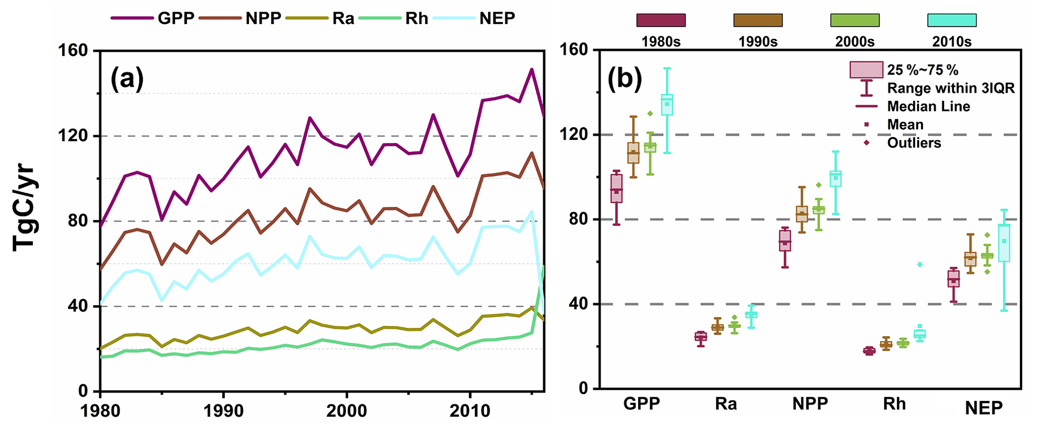
Figure 5 Carbon fluxes simulated by ISAM. (a) The time series of fluxes from 1980–2016. (b) Decadal averages of fluxes.

The spatial trends of the fluxes over 36 years were examined. Figure 6 depicts the difference in the linear trend of total carbon uptake by spring wheat between the 2010s and 1980s. The linear trend was calculated at each grid point using singular spectrum analysis (Golyandina et al., 2013). The difference between the calculated trend line at each grid between the 2010s and 1980s gives us the total change in carbon fluxes over the period. The stippling in the figure shows the grids with significant trend signals from 1980–2016, calculated at a significance level of 95 %. The results show that the Indo-Gangetic Plain (IGP) region of India saw a significant increase in GPP than all other regions over the 37-year period. We can also observe a slight decrease in GPP in the western region. A similar trend in TER is observed, but the magnitude is less than that of GPP. The total carbon taken up by the spring wheat during the growing season is given by NEP, and the figure shows no significant increase in carbon uptake in the southern and northwestern parts. However, the IGP, along with Punjab and Haryana, has a significant increase in carbon uptake. Figures 5 and 6 highlight how the carbon uptake by spring wheat has changed over 3 decades and the spatial variation in this trend. The impact of climatic and management practices causing the above-observed trends is analyzed in the next section.

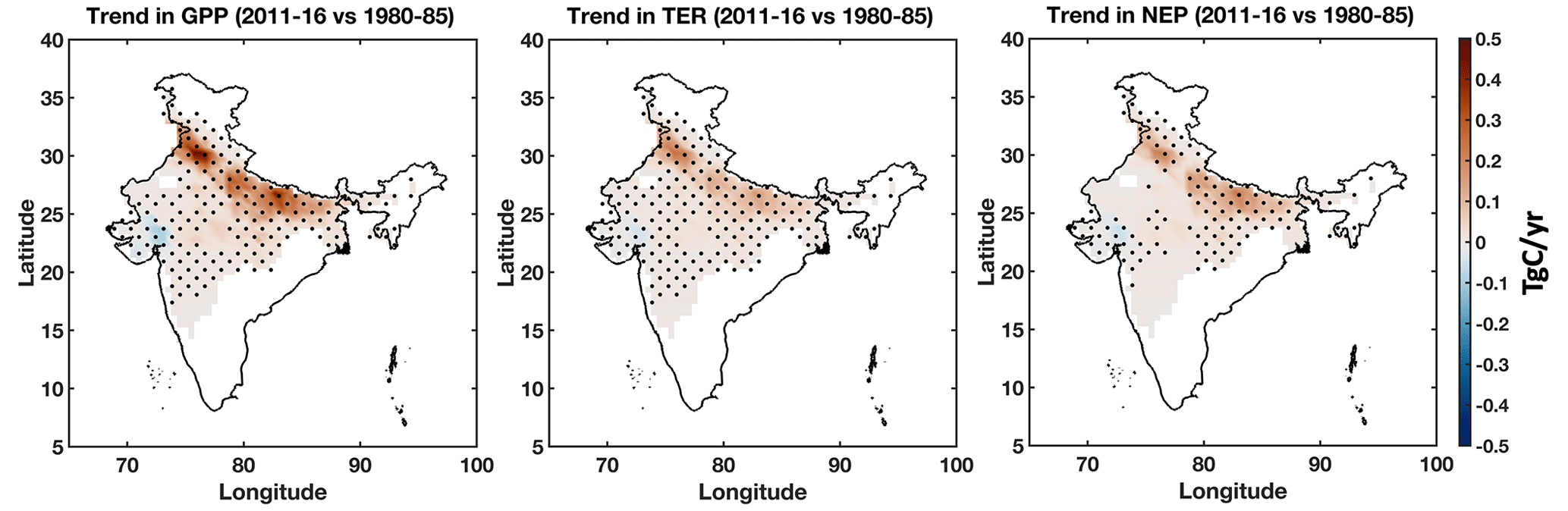
Figure 6 The difference in carbon fluxes (the 1980s vs. 2010s). The stippled regions have a trend signal significant at 95 %.

3.4 Effects of external drivers on carbon fluxes

We investigated the impact of two climate drivers, changing temperature and [CO₂], as well as two agricultural practices, nitrogen fertilizer and water availability due to irrigation, on carbon fluxes from spring wheat croplands. Figure S4 depicts the variation of these variables. Figure S4a shows the temperature anomaly between S_CON and S_Temp. The temperatures are always warmer in S_CON compared to S_Temp. During the study period, the temperature anomaly increased at 0.038 ^∘C yr⁻¹ (Fig. S4a). [CO₂] has also shown a consistent rise and increased at 1.743 ppm yr⁻¹ (Fig. S4b). The nitrogen fertilizer added to the C₃ crops increased at 1.86 kg ha⁻¹ yr⁻¹ over 36 years from 1980–2016 (Fig. S4c) (Hurtt et al., 2011). Figure S4d displays the anomaly in water in the root zone during the growing season, estimated as the difference between S_CON and S_Water. Irrigation increases the water available to crops during the growing season in the S_CON run. The S_CON run provides ∼ 120 mm per season more water to the crop than the S_Water run, which is ∼ 50 % of the wheat crop water requirement during the growing season.

The effects of these factors are estimated by analyzing the difference in simulated carbon fluxes between the control and experimental simulation (Fig. 7 and Table 4). Results show that the increase in temperature has a negative effect on all the fluxes. The temperature anomaly rose at 0.038 ^∘C yr⁻¹, and yearly GPP decreased at 0.597 TgC yr⁻¹² during the study period. The mean temperature anomaly during the growing season in each decade is 0.25, 0.67, 1.43, and 0.9 ^∘C. The temperature varied less between the 1980s and 1990s. Therefore, a slight difference in median GPP between these two decades is observed (Fig. 7a). However, a higher spread in the box–whisker plot of GPP is observed in the 1990s, which reflects a few growing seasons with considerable high-temperature variation. The higher temperatures during the 2000s and 2010s caused a significant decrease in GPP. Since the temperatures varied considerably during the 2000s and 2010s, a large spread in simulated GPP can be observed. Similar trends in NPP and NEP can be observed with a decrease of 21.9 and 13.9 TgC yr^−1 ∘C⁻¹ rise in temperature. Due to a temperature rise, the growing period and the crop phenology shorten (Koehler et al., 2013; Sonkar et al., 2019), which is also simulated by ISAM (Figs. S5a and S6a). Hence a decrease in fluxes is observed. As the crop growth decreases, the TER and NEP also decrease.

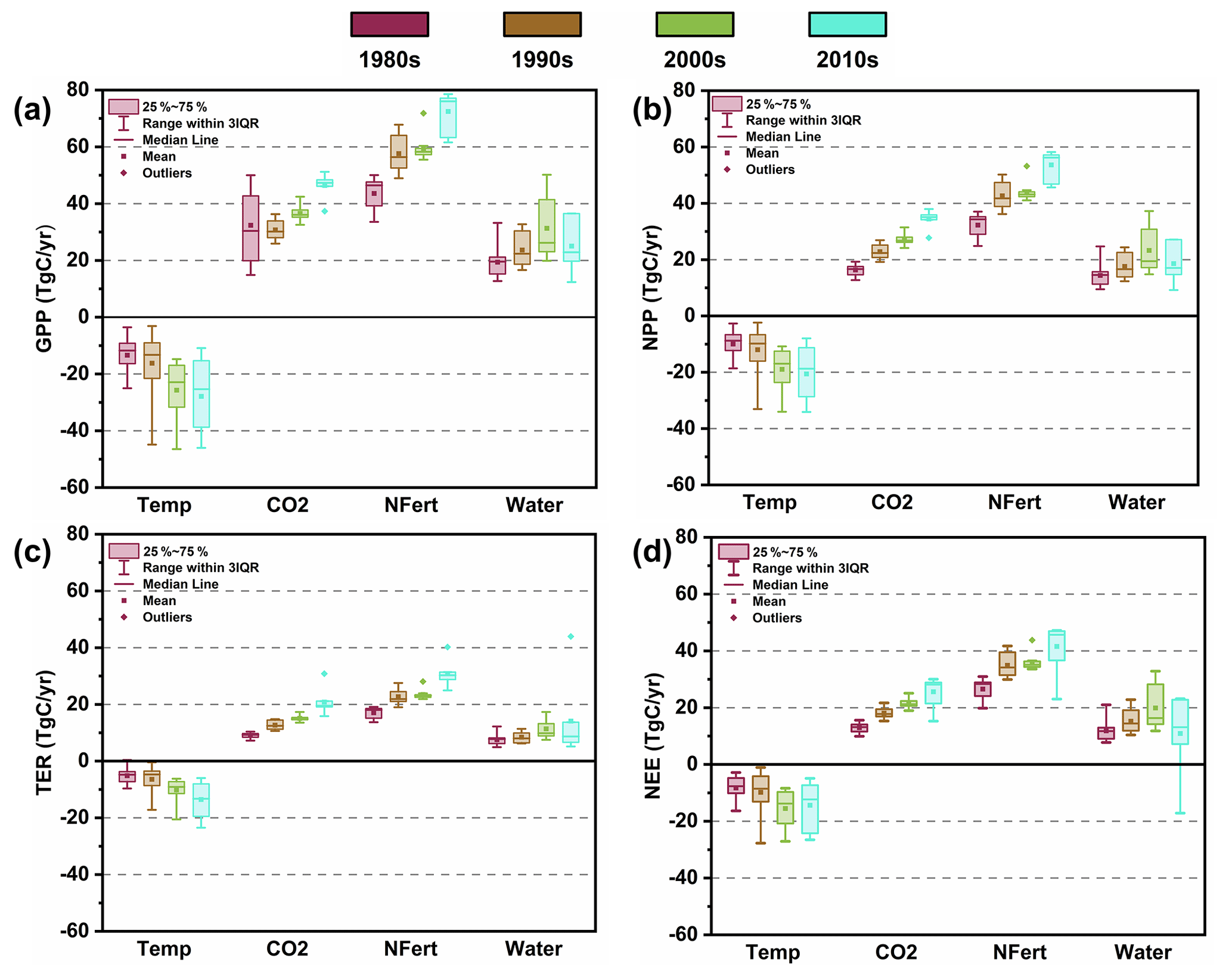
Figure 7 The impact of various drivers (temperature and CO₂, as well as agricultural practices: nitrogen fertilization and water added through irrigation) on wheat carbon fluxes. The impact of temperature is S_CON−S_Temp. Similarly, the impact of CO₂ is $S_{\mathrm{CON}}-S_{{\mathrm{CO}}_{\mathrm{2}}}$, nitrogen fertilization is S_CON−S_{N_Fert}, and water added through irrigation is S_CON−S_Water. The variation in the impact of each variable across each decade is shown in box–whisker plots.

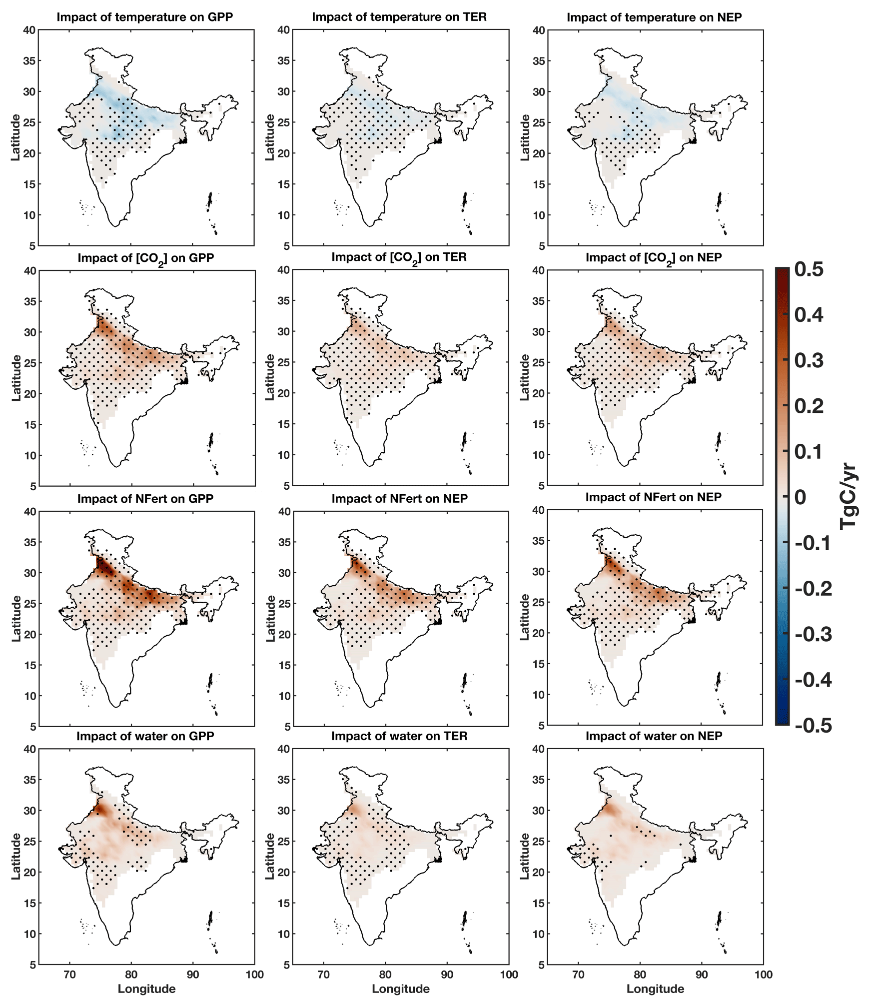
Figure 8 Spatial variation in the impact of temperature, [CO₂], nitrogen fertilization, and water added to spring wheat on the GPP, TER, and NEP.

We analyzed the spatial variation in the impact of temperature on the GPP, TER, and NEP (Fig. 8). The figure shows the impact of temperature (S_CON−S_Temp) averaged from 1980–2016. The stippling in the figure shows the grids with significant trend signals from 1980–2016, calculated at a significance level of 95 %. The temperatures in S_Temp are the de-trended climatological values from 1900–1930. Figure S4 shows the anomaly in growing season temperatures between the S_CON and S_Temp simulations. We observe that the higher temperatures in the S_CON run caused a decrease in carbon taken up by the spring wheat compared to the lower temperatures in the S_Temp run. However, the carbon uptake decrease is inconsistent across the wheat-growing regions. The IGP, Punjab, Haryana, and a few parts of central India are primarily affected by the higher temperatures, while the impact is less in other regions. Interestingly, only some trend signals are significant at 95 %, especially in the eastern IGP, Punjab, and Haryana. The trend in the impact of the temperature of TER is consistent over most wheat-growing regions, although the magnitude is less. The impact on NEP due to higher temperatures is consistently negative across the wheat-growing regions but insignificant in the IGP, Punjab, and Haryana. This behavior in these regions might be because these areas are highly irrigated.

Results showed that the increase in [CO₂] alone has led to a rise in annual GPP, NEP, R_a, and R_h of 0.805, 0.422, 0.201, and 0.175 TgC yr⁻¹², respectively (Table 4). During the study period, [CO₂] rose at 1.743 ppm yr⁻¹, causing an increase in GPP by 462 GgC yr⁻¹ for a unit parts per million (ppm) rise in [CO₂]. The GPP had a consistent rise each decade (Fig. 7). A large spread in GPP was observed in the 1980s. The [CO₂] has consistently increased (Fig. S4b), but the temperature anomaly in the 1980s was below zero for a few growing seasons (Fig. S4a). Therefore, significant variation in GPP and other fluxes was observed (Fig. 5a) in this decade. Similarly, due to higher CO₂ availability for the wheat crops, NPP, NEP, and TER increased by 202, 100, and 173 GgC yr⁻¹ per part per million rise in [CO₂]. As the [CO₂] level increases in the environment, more carbon is available for crop uptake by photosynthesis (Saha et al., 2020). Analyzing the spatial variation in the impact of [CO₂] (Fig. 8), we observe that the higher [CO₂] in S_CON led to higher carbon uptake across all the wheat-growing regions, with a higher impact observed in the IGP, Punjab, and Haryana. The impact of [CO₂] is significant in all the wheat-growing regions. Similar trends in TER and NEP are observed, although with a lower magnitude.

Nitrogen fertilization increased NEP, R_a, and R_h at 0.468, 0.231, and 0.197 TgC yr⁻², respectively. The impact of nitrogen fertilization on GPP at 0.897 TgC yr⁻² was the highest among all the factors. Nitrogen fertilization caused an increase in GPP by ∼ 33 TgC on an annual basis. Similarly, NEP increased by ∼ 17 TgC yr⁻¹, and R_a and R_h increased by by ∼ 8 and ∼ 7 TgC yr⁻¹, respectively. Nitrogen fertilization is essential in India due to its tropical climate and multiple cropping systems (Gahlot et al., 2020). Studies have shown that nitrogen availability impacts carbon uptake through progressive nitrogen limitation (Jain et al., 2009). Though progressive nitrogen limitation is observed over longer timescales than the growing period of the crops, the decadal carbon flux simulations revealed some exciting results. Even under excess [CO₂], if nitrogen is limited, crop growth does not show a significant difference, but a decrease in carbon uptake is observed (Jain et al., 2009; Luo et al., 2006). Under excess [CO₂], if sufficient nitrogen is available, the ecosystem's carbon uptake increases; therefore, the maximum flux increase was observed in the nitrogen fertilization case (Table 4 and Fig. 8). The study by Lin et al. (2021) focusing on maize and soybean crops emphasized the importance of fertilization to improve crop growth, and our study proves that with adequate fertilization, even the spring wheat in the Indian region also grows well and the carbon uptake is higher. Nitrogen fertilization was consistent over the decades, leading to a constant rise in GPP. However, the variation in GPP in the 2000s was the least (Fig. 7) influenced by high temperatures during this decade (Fig. S4). A similar pattern of low variation was observed in NEP, R_a, R_h, and NEP during this period. The spatial variation across wheat-growing regions in the impact of nitrogen fertilization reveals the same pattern as seen in $S_{{\mathrm{CO}}_{\mathrm{2}}}$. However, the impact on carbon fluxes is more significant due to nitrogen fertilization than CO₂. A higher impact was observed in the IGP and adjoining regions, which are highly cultivated and irrigated. The results show that using nitrogen fertilization improves the carbon uptake by spring wheat, in line with earlier studies (Jain et al., 2009; Luo et al., 2006).

Table 4 The impact of each driver (TgC yr⁻²) on various fluxes of the spring wheat crop in India. The values show the slope, giving the linear trend of individual fluxes. ^* The trend has a significance level of p<0.01.

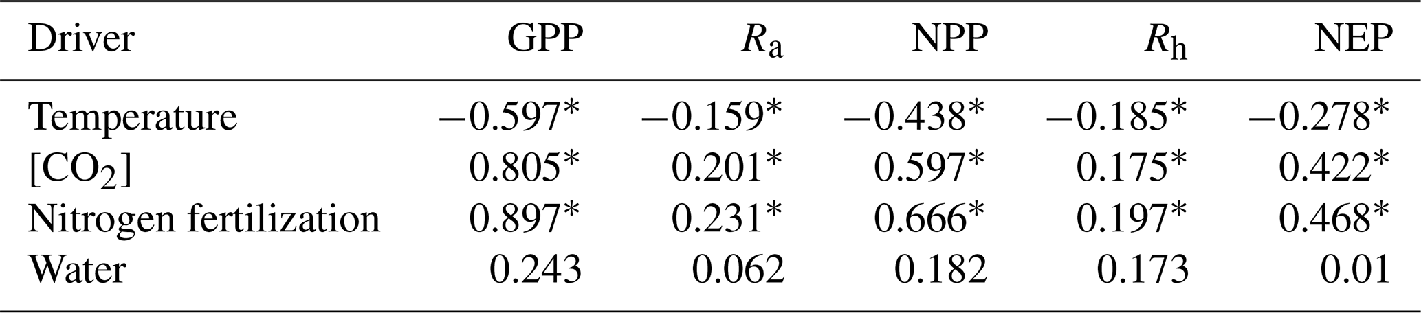
The impact of water added to the crop led to an annual increase of ∼ 9 TgC in GPP, ∼ 6.5 TgC in NPP, ∼ 2 TgC in R_a, and ∼ 6 TgC in R_h. The reason for the small trend was the fluxes increasing through the 1980s, 1990s, and 2000s but declining in the 2010s. The decline in the 2010s was due to less water availability for the crops during this period, as shown in Fig. S4d, hence affecting the trends in the fluxes (Table 4). The higher GPP, NPP, and NEE in the 2000s compared to the 1990s, even though the temperatures were higher in the 2000s, suggests that the adverse effects of high temperatures can be overcome if the crops are provided with enough water. Studies like Hatfield and Prueger (2015) and Green et al. (2019) explored the impact of water availability in terrestrial ecosystems on carbon fluxes. They concluded that higher water availability improves the carbon uptake in terrestrial ecosystems. The spatial variation analysis (Fig. 8) shows that the higher water availability in the S_CON run caused higher carbon uptake throughout the wheat-growing regions. The highest impact is observed in the northwestern regions of the country (Punjab and Haryana), which are highly irrigated, and most of the crop water requirements are met through irrigation. However, the stippling, which shows if a region has a significant trend over the 36 years, reveals that most wheat-growing regions do not have a significant increasing or decreasing trend. Nevertheless, the impact of adequate water causing higher carbon uptake by spring wheat is evident in Fig. 8.

4 Discussion

ISAM simulations, particularly numerical experiments examining the effects of temperature, [CO₂], nitrogen fertilization, and irrigation, revealed some intriguing features of India's spring wheat agroecosystem. All the fluxes follow a similar pattern of a high rise from the 1980s to the 1990s, a slight increase from the 1990s to the 2000s, and a steep rise from the 2000s to the 2010s (Fig. 5b). The [CO₂] and nitrogen fertilization increased throughout the study, whereas temperature and irrigation varied irregularly (Fig. S4). The impact of [CO₂] as measured by the difference between S_CON and $S_{{\mathrm{CO}}_{\mathrm{2}}}$ highlighted that with higher [CO₂], the carbon taken up by wheat increases, and the overall ecosystem exchange from croplands is more significant than in the low [CO₂] case. The findings from the spring wheat agroecosystem align with studies such as Yoshimoto et al. (2005) and Saha et al. (2020), who studied broader ecosystems. During the 2000s, there was a sudden drop in fluxes (Fig. 5a), which coincided with the higher temperature anomaly of 1.43 ^∘C (Fig. S4a). Patel et al. (2021) also found a negative relationship between NEP and temperature, owing to higher respiratory losses at higher temperatures. Sonkar et al. (2019) and Koehler et al. (2013) reported similar behavior of spring wheat in warmer temperatures. However, the added water during the 2000s mitigated the negative impact of higher temperatures, as evidenced by the positive impact of water observed during this decade (Fig. 7a–d). The positive impact of water in the 2000s is more significant than in the 1990s, despite the temperature anomaly in the 2000s being 1.43 ^∘C compared to 0.67 ^∘C in the 1990s. Therefore, the study suggests that providing adequate water through irrigation can mitigate the adverse effects of high temperatures.

Our spatial variation analysis of carbon fluxes and the impact of climate variables and management practices shows that the most significant carbon uptake by spring wheat is from the IGP and the northwestern regions. This is because these regions are highly cultivated and irrigated, and they are the major wheat producers of India. Interestingly, the effect of nitrogen fertilization on carbon fluxes was high among all the variables considered. Irrigation was another critical factor affecting crop growth and carbon fluxes. The experiments with detrended temperature (S_Temp) revealed that the crops' sowing date and growing lengths are affected by temperature variation (Figs. S6 and S7). The growing season is shorter by nearly a week to 2 weeks in S_CON, reducing the carbon fluxes during the growing season (Fig. 8). The dynamic sowing date does an excellent job of adjusting to the changes in climatic variables like temperature and precipitation (Figs. S3 and S5a, d). The drivers for decision-making in the sowing of crops by the farmers in India are mainly temperature and rainfall. Therefore, building a model replicating human decisions will play a crucial role in analyzing the impacts of future climate on spring wheat.

The simulated carbon fluxes are comparable to published values. The cumulative GPP and NEP for the wheat-growing season observed at the Saharanpur site are 621 and 192 gC m⁻² (Patel et al., 2021). The GPP and NEP values simulated at the IARI site are 729.9 and 523.3 gC m⁻². Although the GPP is comparable with Patel et al. (2021), NEP values simulated by ISAM are not in the same range. The higher NEP is because the ratio of R_a to GPP is low in our case compared to many studies on spring wheat. Amthor and Baldocchi (2001) reported a R_a GPP⁻¹ range of ∼ 0.3–0.6 for crops like wheat. Our value of 0.26 is slightly lower than that. Many studies (Table S2) report an R_a value of ∼ 0.5 GPP. These are all winter wheat with a vernalization period and a growing length of more than 200 d; in our case, it hardly exceeds 150 d. Interestingly, Zhang et al. (2020), who reported R_a values like ours, also consider full irrigation like our study, while the other studies do not consider irrigation. Comparing the R_a GPP⁻¹ from S_Water we observed that the value is 0.3 and in the range proposed by Amthor and Baldocchi (2001). Therefore, our findings prove that highly irrigated fields will have lower respiration losses.

Additional research is needed to address some of the study's limitations. The model evaluation is very important for studies like this. Multiyear data from multiple stations across the study domain should be used for evaluation. We built a dataset for spring wheat consisting of crop phenology and yield for nine sites and 26 growing seasons. The crop phenology and yield data are used to evaluate the model. However, carbon flux observations from cropland in India are not publicly available. We evaluated the carbon fluxes simulated by ISAM using data from three experimental agricultural sites in northern India. Even though the model evaluation was suboptimal regarding carbon fluxes, this study is a step in the right direction because it is the first to use site-scale observations to evaluate all terrestrial carbon fluxes simulated by a process-based model.

Second, we estimated the effect of water availability on carbon fluxes by comparing the control simulation S_CON, where the crops do not experience any water stress, with the S_Water simulation, where no irrigation is applied. The best way to understand the effect of irrigation would be to conduct simulations driven by actual irrigation data. For this purpose, we need a gridded irrigation time series dataset. Unfortunately, such data do not exist (Gahlot et al., 2020) or are unrealistic in magnitude and timing (Mathur and AchutaRao, 2020). Many studies show that using different cultivars can change spring wheat yield, but there are no studies on the effects on carbon fluxes. Thus, studying the impact of cultivars on carbon fluxes is an exciting and open question. This effect was not incorporated into our study. The spatiotemporal maps of cultivar use and site-scale carbon flux and phenology data for various cultivars will take a lot of work to develop. The community should strive to create such datasets to better understand and simulate different cultivars' effects.

Finally, our simulations were run with a land model driven by externally imposed forcings. We ignored the feedback between the land surface and the atmosphere, which can be significant, especially for natural drivers like [CO₂] and temperature. The next step would be to use a coupled land–atmosphere model that includes feedback between the terrestrial and atmospheric components of the carbon cycle.

5 Conclusions

We used ISAM equipped with a spring wheat module to study the carbon fluxes in spring wheat agroecosystems across the wheat-growing regions of India for the last 4 decades. The ISAM spring wheat module ISAM_{dyn_wheat} simulated the temporal patterns of GPP, TER, and NEP at the site scale for the IARI experimental wheat farm. The main conclusions from this study are as follows.

• Carbon fluxes in spring wheat agroecosystems varied widely across the country due to divergent climatic conditions and management practices, primarily due to differences in planting dates. While the central and eastern parts of the spring wheat-growing regions showed high carbon fluxes during January, the northern parts exhibited their maximum carbon flux values during March.

• The effects of increasing [CO₂], nitrogen fertilization, and irrigation led to positive trends in carbon fluxes in the last 4 decades. Nitrogen fertilization had the strongest effects, followed by [CO₂] and water availability. Providing sufficient fertilizers and water through irrigation may counteract the adverse effects of high temperatures.

• The limitation on water available through irrigation in the future in regions like Punjab and Haryana might adversely affect the spring wheat growth and, as a result, the carbon fluxes from this agroecosystem.

Understanding the variability in terrestrial carbon fluxes is essential for understanding the carbon cycle. Agroecosystems cover large parts of the terrestrial biosphere, with the spring wheat agroecosystem being one of India's most extensive land use types. This paper is one of the first long-term regional-scale studies to examine carbon dynamics in an Indian agroecosystem. After appropriate calibration, the model developed in this study can also be used to study other agroecosystems. Very importantly, it can serve as a tool to conduct numerical experiments to study future scenarios and the effects of external drivers. Thus, this study will likely be crucial in advancing our understanding of terrestrial carbon dynamics and our ability to simulate their behavior.