Understanding pattern scaling errors across a range of emissions pathways

The regional climate impacts of hypothetical future emissions scenarios can be estimated by combining Earth system model simulations with a linear pattern scaling model such as MESMER (Modular Earth System Model Emulator with spatially Resolved output), which uses estimated patterns of the local response per degree of global temperature change. Here we use the mean trend component of MESMER to emulate the regional pattern of the surface temperature response based on historical single-forcer and future Shared Socioeconomic Pathway (SSP) CMIP6 (Coupled Model Intercomparison Project Phase 6) simulations. Errors in the emulations for selected target scenarios (SSP1–1.9, SSP1–2.6, SSP2–4.5, SSP3–7.0, and SSP5–8.5) are decomposed into two components, namely (1) the differences in scaling patterns between scenarios as a consequence of varying combinations of external forcings and (2) the intrinsic time series differences between the local and global responses in the target scenario. The time series error is relatively small for high-emissions scenarios, contributing around 20 % of the total error, but is similar in magnitude to the pattern error for lower-emissions scenarios. This irreducible time series error limits the efficacy of linear pattern scaling for emulating strong mitigation pathways and reduces the dependence on the predictor pattern used. The results help guide the choice of predictor scenarios for simple climate models and where to target for the introduction of other dependent variables beyond global surface temperature into pattern scaling models.

1 Introduction

Anthropogenic climate change has already driven significant impacts throughout the globe, and these will continue to become more severe (IPCC, 2021). Estimates of the climatic impacts of future emissions depend on several sources of uncertainty – internal variability, model structural uncertainty, and unknowns in the emissions themselves (Hawkins and Sutton, 2009). The first two sources of uncertainty are often explored using multi-member ensembles of Earth system models (ESMs). The emissions uncertainty can only be explored by constructing multiple hypothetical future emissions scenarios, and investigating their respective impacts (Riahi et al., 2022).

The most recent generation of integrated assessment model (IAM)-simulated scenarios are the Shared Socioeconomic Pathways (SSPs; Gidden et al., 2019). These have been used in ESMs to assess the future climate response in the contribution of Working Group I (WGI) to the Sixth Assessment Report of the Intergovernmental Panel on Climate Change (AR6 IPCC; Lee et al., 2021). ESMs are computationally expensive to run, so in general they can only simulate a handful of future emissions scenarios (O'Neill et al., 2016; Tebaldi et al., 2021). The small number of scenarios used for ESM simulations can mask uncertainties in future pathways, as the full range of the parameter space for plausible emissions is not adequately sampled (Grubler et al., 2018; Otero et al., 2020; Partanen et al., 2018). Accurate simplified methods which allow a good understanding of the regional impacts of novel emissions scenarios are therefore highly motivated in order to explore a broader range of emissions pathways than currently possible with comprehensive ESMs.

Both the IPCC WGI and Working Group III (WGIII) AR6 reports used simplified physical climate model emulators trained on more complex ESM simulations to assess possible future projections of global surface temperature (Lee et al., 2021; Forster et al., 2021; Riahi et al., 2022; Kikstra et al., 2022). However, the assessment of regional climate projections relied largely on simulations from ESMs and regional climate models (RCMs). Since the United Nations Framework Convention on Climate Change (UNFCCC) 2015 Paris Agreement, which frames international climate goals in terms of global temperature targets, there has been growing emphasis on examining climate change impacts as a function of the global warming level (IPCC, 2018). For example, in IPCC AR6, future scenarios simulated by ESMs were compared at different global mean temperature levels (Lee et al., 2021; Seneviratne et al., 2021). The suitability of this approach depends on the extent to which regional changes scale with global temperature change, which in turn depends on the variable of interest and the details of the greenhouse gases (GHGs) and aerosols scenario. Regional statistical emulation tools operate on a similar basis, using techniques such as pattern scaling to translate simple large-scale information such as global mean temperature into estimates of the spatially resolved climate response for a broad range of scenarios (James et al., 2017; Mitchell et al., 1999; Osborn et al., 2018).

Pattern scaling approaches can be limited by systematic response variations between and within scenarios. The radiative forcing from long-lived species is independent of the emissions location, but the impacts of short-lived species such as aerosols strongly depend on the pattern of emissions, with typically larger effects occurring locally (Liu et al., 2018; Persad and Caldeira, 2018). The patterns of climate change impacts also differ between transient and equilibrium climate states; the transient temperature response is typically larger over land than over ocean, due to the greater thermal inertia of the latter (Herger et al., 2015; Huang et al., 2020; King et al., 2020; Mitchell, 2003). These two factors – variations in the forcing pattern and the level of disequilibrium – can be expected to break the linearity assumed within pattern scaling if they differ between and within scenarios (Goodwin et al., 2020; Herger et al., 2015; James et al., 2017; Mitchell, 2003; Osborn et al., 2018). Pattern scaling has been modified to partially address these issues by using patterns varying between forcers (Kravitz et al., 2017; Xu and Lin, 2017; Schlesinger et al., 2000) and the response timescale (Zappa et al., 2020).

Other non-linearities in climate response can occur, especially under higher-emissions scenarios (Lopez et al., 2014); for example, the removal of sea ice in the Arctic will saturate the sea ice–albedo feedback and reduce the local temperature sensitivity (Huang et al., 2020; Lynch et al., 2017), though higher sensitivity may initially occur due to sea ice thinning (Ishizaki et al., 2012). Some responses of the climate system to external forcing, such as sea ice retreat and intertropical convergence zone shifts, move geographically and will therefore be poorly represented by pattern scaling (Herger et al., 2015).

Despite the potential limitations of pattern scaling for climate emulation, the technique has been shown to work well across a range of scenarios (Alexeeff et al., 2018; Beusch et al., 2020; Mitchell et al., 1999). A linear approximation has been found to be reasonable for regional temperature changes within and between sets of scenarios (Seneviratne et al., 2016; Seneviratne and Hauser, 2020), with similar response patterns found within different emissions scenarios in the near-term (Lee et al., 2021). The variation in response patterns between scenarios is typically less than the variation between models, indicating that the errors arising from pattern scaling are smaller than model uncertainty (Goodwin et al., 2020; Herger et al., 2015; Osborn et al., 2016, 2018; Tebaldi and Arblaster, 2014; Tebaldi and Knutti, 2018). Pattern scaling errors are generally substantially larger when extrapolating (projecting a scenario with higher forcing than the data used to generate the pattern) than when interpolating (Herger et al., 2015; Mitchell, 2003; Tebaldi et al., 2020; Beusch et al., 2022a), with smaller errors for more modest forcing differences between the predictor and target scenarios (Osborn et al., 2018).

Pattern scaling has been used to emulate regional changes in temperature (Beusch et al., 2020; Link et al., 2019), to forecast temperature and precipitation simultaneously (Snyder et al., 2019), and in order to study changes in extreme precipitation (Thackeray et al., 2022). The application of pattern scaling to precipitation is complicated relative to temperature by the larger role of internal variability (Hawkins and Sutton, 2011), the presence of strong non-linearities and local factors (Liu et al., 2023), and the role of forcing-specific adjustments (Myhre et al., 2018). However, extreme precipitation is more closely constrained by moisture availability and may be more successfully emulated through pattern scaling (Pendergrass et al., 2015; Sillmann et al., 2017). Pattern scaling has also been incorporated with Earth system components such as land surface models to make faster projections (Zelazowski et al., 2018). It has been applied to estimate the regional effects of single-country GHG emissions in order to attribute their local temperature impacts (Beusch et al., 2022b) and to estimate the country-level economic impacts attributable to each other country's CO₂ emissions (Callahan and Mankin, 2022). These exercises would require vast computer resources and time if they were attempted with ESMs.

The scenarios to which pattern scaling has generally been successfully applied typically have smaller inter-scenario variation in aerosol emissions and warming rates than more recent, and likely future, scenarios of interest. Many historical studies applied pattern scaling to the CMIP5-era Representative Concentration Pathway (RCP) scenarios (Alexeeff et al., 2018; Goodwin et al., 2020; Herger et al., 2015; Ishizaki et al., 2012; Kravitz et al., 2017; Lynch et al., 2017; Osborn et al., 2018; Tebaldi et al., 2020; Tebaldi and Arblaster, 2014; Xu and Lin, 2017), which all exhibit similar decreases in anthropogenic aerosol emissions into the future (Gidden et al., 2019), resulting in a much narrower range than projected among the newer SSP scenarios used in CMIP6. This may make the SSP scenarios less amenable to pattern scaling than prior scenarios (Goodwin et al., 2020). The SSP scenarios include SSP1–1.19, approaching the 1.5 ^∘C level under the Paris Agreement (Meinshausen et al., 2020) with stronger mitigation than the RCPs. Many low-emissions Paris-agreement-consistent scenarios were assessed as part of IPCC AR6 WGIII (IPCC, 2022), but relatively few have been systematically studied in multi-ESM projects. Low-emissions scenarios may also encounter issues due to contamination by internal variability in the pattern-generation regression, and stabilisation scenarios may be more susceptible to physical non-linearities (Osborn et al., 2018). Indeed, many studies that find pattern scaling to be accurate with earlier scenarios note that under stronger mitigation or wider ranges in aerosol emissions, the technique would be less effective (Alexeeff et al., 2018; Mitchell et al., 1999; Tebaldi and Arblaster, 2014).

While tools such as MESMER (Modular Earth System Model Emulator with spatially Resolved output) have been developed to implement pattern scaling using the SSP scenarios (Beusch et al., 2020), particularly studying the reproduction of scenarios from their own pattern (self-emulation), a systematic analysis of the range of errors associated with the application of pattern scaling to temperature within the SSPs remains to be done. Multi-model studies analysing pattern scaling efficacy for low-emissions scenarios are also lacking (Tebaldi and Knutti, 2018). The effect of the choice of predictor data used to generate the pattern utilised in pattern scaling has also not been fully explored. This paper takes steps to address these gaps through a novel decomposition of pattern scaling errors into their relation to pattern scaling assumptions.

This paper studies the effects of the pattern scaling assumptions on regional temperature projections, decomposing the pattern scaling error into the following two components relating to space and time (see Sect. 2.3):

• i.

  The pattern assumption, in which pattern scaling assumes that the pattern of change is constant between all scenarios, regardless of the mix and level of forcers within them.

• ii.

  The time series assumption, in which pattern scaling assumes that the time series response at each location follows the same shape as the global response and is simply modified by the local sensitivity (i.e. the pattern), thus allowing the local change time series to be estimated by scaling the global time series by a constant local pattern coefficient. This can be thought of as assuming the pattern is constant in time within a given scenario.

We explore how these errors vary when projecting different emissions scenarios, and the effect of different choices of (one or more) predictor scenario(s), to determine the impacts of this decision on emulation accuracy. Inter-model variation is investigated for all the impacts studied.

Section 2 sets out the ESM data utilised and the model used to perform the pattern scaling analysis and shows how to diagnose the error associated with each pattern scaling assumption. Section 3 presents the key results, Sect. 4 explores the implications for the application of pattern scaling, and Sect. 5 provides discussion and conclusions.

2 Methods

2.1 Earth system model data

Two sets of emissions pathways are the focus of this paper. To understand the effect of different forcers on the warming pattern and pattern scaling errors, two historical (1850–2020) scenarios from the Detection and Attribution Model Intercomparison Project (DAMIP; Gillett et al., 2016) project are used, namely hist–aer, which includes only anthropogenic aerosol emissions, and hist–GHG, which includes only greenhouse gas emissions. This allows for an idealised comparison of the different patterns attributable to historical levels of different forcers, although neither represents a realistic emissions pathway due to the co-emissions of aerosols and GHGs in reality. To determine the difference between warming patterns amongst coherent emissions pathways, the SSP scenarios are used, examining several SSPs but focussing on SSP1–1.9 and SSP5–8.5, with data for both taken from 2015–2100.

Data for all scenarios were taken for annual mean temperatures from the CMIP6ng database (Brunner et al., 2020), which re-grids all data to a common 2.5^∘ × 2.5^∘ latitude–longitude grid to allow for inter-model comparison. For each of the two sets of emissions pathways, all models with at least one member of each experiment were used, including 10 ESMs for the 2 DAMIP scenarios and 8 ESMs for the 5 SSPs. The models and members for each scenario are given in Table S1 in the Supplement. Inter-model results are averaged first over each model ensemble, with this model average then being compared to avoid weighting by the ensemble size of each model.

2.2 Pattern scaling methodology

This study utilises the mean response component of the MESMER model (Beusch et al., 2020), implementing pattern scaling to emulate the spatial annual mean temperature response in a scenario. While both pattern scaling and the time shift method – which selects a window of data centred around the year in which the global average reaches a desired global warming level – generate accurate emulations and out-of-sample mean emulations, pattern scaling has been found to perform slightly better in some metrics (Tebaldi et al., 2020).

The pattern is derived from linear regression of the local response time series on the global response at each grid cell. The full time series is regressed for each pattern (i.e. 1850–2020 for hist–aer and hist–GHG; 2015–2100 for SSP1–1.9 and SSP5–8.5), with anomalies calculated relative to the first 50 years of each experiment. This linear regression approach to pattern scaling has been shown to provide more accurate patterns than the alternative delta method, whereby the average climate towards the end of a scenario is subtracted from that in the early period (Lynch et al., 2017; Mitchell, 2003).

In the default configuration of MESMER, the raw annual grid-cell-level data are regressed against smoothed global temperatures, but here this is modified to use the same smoothing on both local and global temperatures. This smoothing prior to regression is performed to ensure that the global average scaling factor is very close to unity (1 $K/K$) when applying the regression to an individual low-emissions scenario such as SSP1–1.9. The weighted global average regression parameter should be 1 by construction when using the global mean of a variable to target the local response of the same variable (in this case temperature), since the global mean is simply the weighted average of the local values. When regressing unsmoothed local data against smoothed global temperatures in a low-emissions scenario that exhibits a peak and decline in temperatures, the regression parameter can be artificially enhanced due to a smoothing of the peak. We therefore use the same smoothing on local and global temperatures before applying the regression. The smoothing performed is locally weighted scatterplot smoothing (LOWESS), which takes the weighted average of the time series across a moving window. The weighting is tricube, and the window fraction set to the default MESMER value of 50 divided by the number of time steps as in the default case. When using the annual mean SSP data here, this is $\mathrm{50}/\mathrm{85}$ ≃ 0.6.

MESMER's default version only includes land grid points in order to focus on land impacts, but here all grid points were used to study the broader response. The intercept of the linear regression is zero in theory, but while it is generally small, in practice it is non-zero and method dependent (Beusch et al., 2020) and is added to the emulation in MESMER. Many models produce multiple ensemble members for a given scenario to reduce internal variability. These members could be averaged over, thus creating a single averaged member, before the regression is applied. Instead, MESMER concatenates the multiple members, stitching the data together into an array for which the total time length is the number of members multiplied by the length of the individual members. A single regression is then applied to this concatenated dataset. Using an ensemble of members reduces the internal variability; the different ensemble sizes used here across models will lead to different levels of variability reduction. Most ensembles used contain greater than three members, but for some model–scenario combinations, only a single member was available (Tables S1 and S2). The full MESMER emulator includes a representation of internal variability at global and local scales, but since this paper focuses on the long-term response, only the pattern scaling (local trends) component is used (Beusch et al., 2020).

A given emulation consists of two components, namely the predictor pattern and the target scenario. The predictor pattern can be derived from one scenario or many, with the regression being applied across the full dataset. The target is a single scenario in each case. The pattern is derived via the linear regression of the local trend on global temperature anomalies, relative to the first 50 years of each predictor scenario. This pattern is then multiplied by the global temperature time series of the target scenario to generate the emulation. The difference between this emulation and the actual ESM pattern is defined as the pattern scaling error. The first 50 years of a given scenario are used as the baseline. The pattern scaling error is zero in the global mean by design – since the pattern (with average value 1) is simply scaled by the global temperature in the ESM – but errors occur regionally, and the global average of the local absolute error will therefore not be zero.

Throughout this paper, the pattern scaling methodology is applied to each model separately. The pattern scaling error is calculated for each model, by subtracting the ESM data from its model-specific emulation. Multi-model means are only taken for plotting, and uncertainties in patterns, emulations, and emulation errors are taken as inter-model standard deviations across the model-specific results.

2.3 Decomposing pattern scaling errors

As described in Sect. 1, the pattern scaling error can be thought of as the deviations from two key assumptions, namely the pattern and time series assumptions. Short-term inter-annual variability is dampened via the LOWESS smoothing, though decadal-scale variability will also be present.

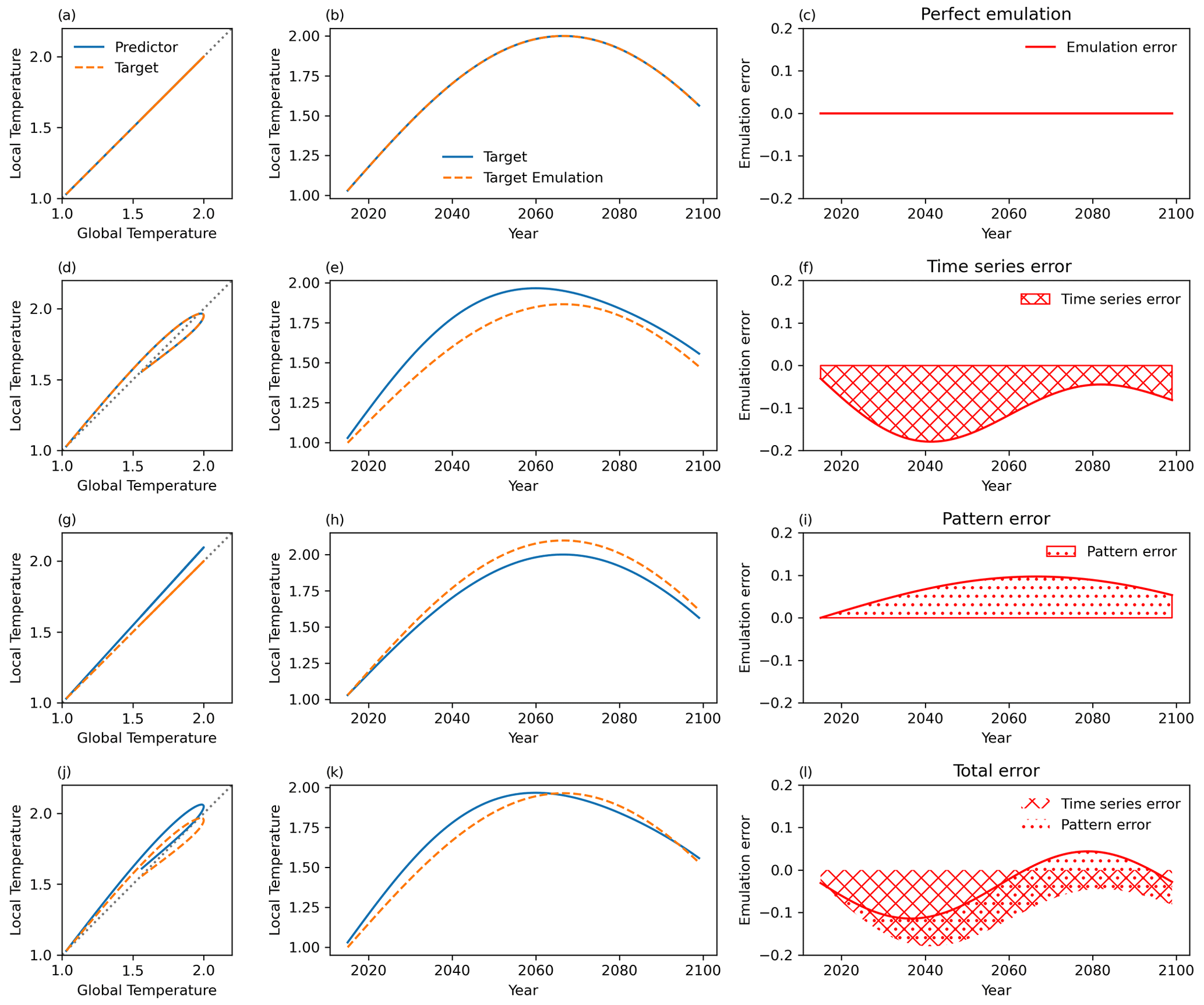
Figure 1 Demonstrating the pattern scaling error decomposition for several idealised scenarios (see the text for details). An idealised scenario is shown in which temperatures relative to preindustrial times rise from 1 K in 2015 to 2 K by 2070 and fall to nearly 1.5 K by 2100. Each row represents a different relationship between the global and local temperature for an arbitrary location, with the left panel indicating the regression of local onto global temperatures, the middle panel the actual and emulated local temperature trajectories, and the right panel the emulation error at this location. (a, d, g, j) Local temperature time series against global. (b, e, h, k) Time series of the target scenario's local response and the emulated local projection. (c, f, i, l) Pattern scaling error time series (i.e. the difference between the emulation and the target scenario in the middle column).

Figure 1 illustrates the decomposition of pattern scaling errors into the pattern and time series errors. Pattern scaling determines the local parameter from the regression of the local on global predictor data and then scales the target global temperature by this value. The pattern scaling error is then the difference between this projection and the actual local response in the target scenario.

Figure 1a–c shows a perfect emulation in which all four of these time series are identical. The scaling parameter is therefore equal between the scenarios (Fig. 1a), and the shape of the emulated response is identical to the target dataset (Fig. 1b), with zero error at all times (Fig. 1c).

The second row in Fig. 1 shows the effect of altering the shape of the local time series but keeping the warming parameter (i.e. the pattern) the same. The scenarios are still identical – the global response and the local response are the same for both – but the shape of the local and global responses within each scenario now differs. In this case, the pattern is correct, and the error is conceptualised as the time series error; that is, the error due to the differing local and global time series response within the scenario. The time mean is not zero, as the time series variability within the scenario modifies the pattern, leading to a non-zero regression intercept and overall emulation errors.

In Fig. 1g–i, the local and global responses are now identical within each time series, but the scenarios themselves are different, as the local parameter of the predictor is larger than in the target. Since the local and global time series in the target scenario follow the same shape, the error is purely due to differences in the scaling parameter, i.e. the local value of the pattern. This error is therefore the pattern error.

Finally, Fig. 1j–l apply both of these changes simultaneously; the local parameter differs between the scenarios, and the local and global time series differ within each scenario, as expected in the real world and ESM data due to non-linearities within the climate system. The total error is comprised of both pattern and time series errors, but the split between them is not clear from the time series.

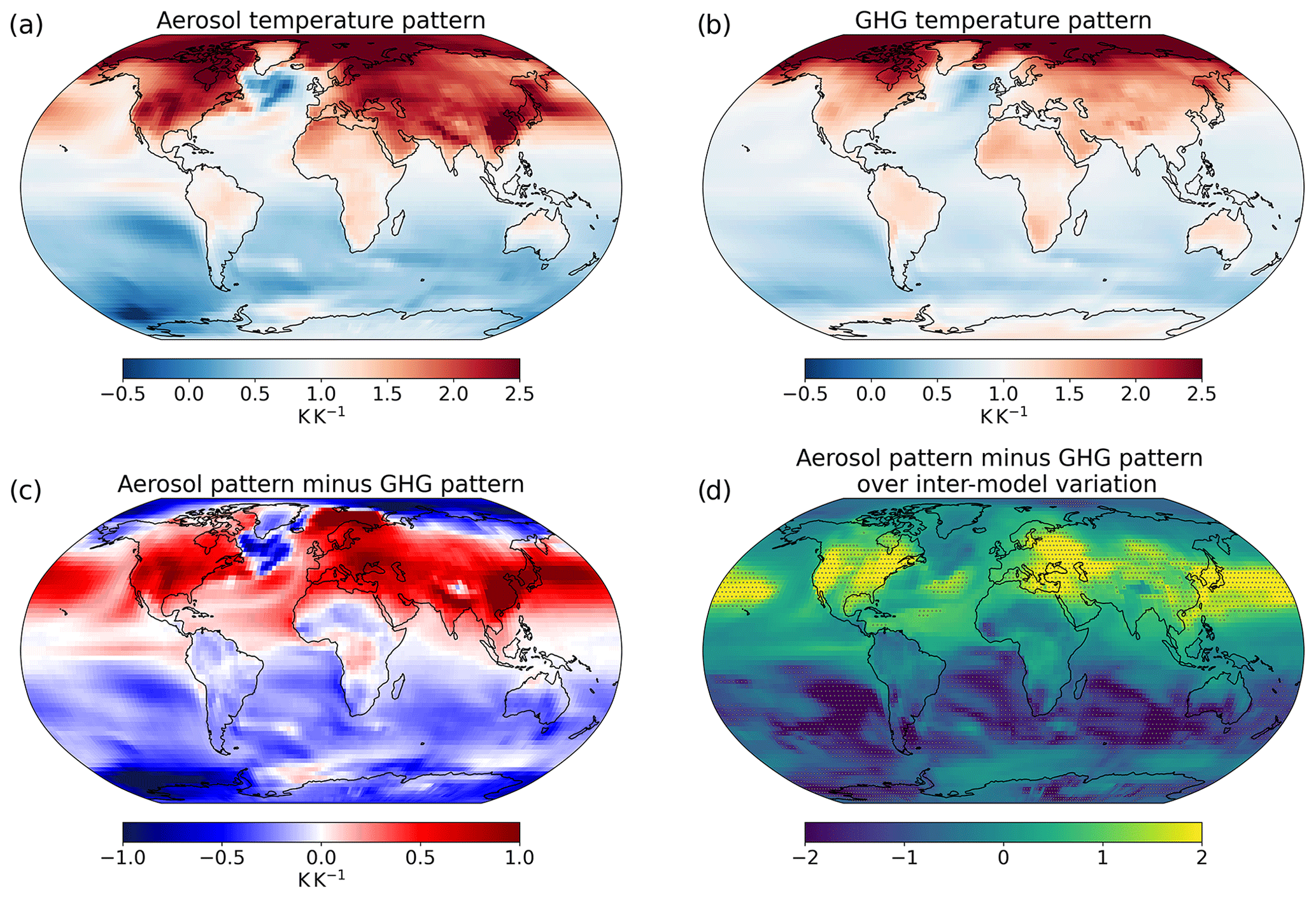
Figure 2 Mean warming patterns across 10 ESMs derived from the historical GHG-only (hist–GHG; a) and aerosol-only (hist–aer; b) simulations, the aerosol pattern minus that from GHGs (c), and this difference divided by the inter-model standard deviation in this difference (d). Panel (d) shows stippling where the multi-model mean difference is greater than 1 inter-model standard deviation. The colour scheme in panels (a) and (d) diverges around 1 (the global average value), with regions which experiences temperature changes weaker than the global mean shown in blue, and areas with a stronger response in red.

Figure 1 illustrates that the general total error, from using one scenario to emulate another, can be decomposed into pattern- and time-series-associated components. The time series error, in row two of Fig. 1, was generated by using the same scenario as the predictor and the target and termed self-emulation. The error is due to the internal dynamics of the response; specifically, this is the difference between the shape of the local and global temperature time series. This error is therefore intrinsic to the target scenario. For a given predictor–target pair, the time series error can be found by calculating the target–target pattern scaling error, i.e. the error upon self-emulation of the target. This can then be subtracted from the original predictor–target pattern scaling error to determine the pattern error. The contribution of each error to the total error can then be studied; the error time series in the bottom row of Fig. 1 shows this decomposition applied to the idealised scenarios.

3 Results

3.1 Effect of pattern error

In this section, the assumption that the pattern is independent of the predictor scenario is investigated, first in the DAMIP experiments and then in the SSP scenarios.

Figure 2a and b show the multi-model mean hist–aer and hist–GHG response pattern based on regression across the whole period (1850–2020). Note that while aerosols drive a cooling, since the local response is regressed against the global mean the sign cancels, with the pattern therefore giving the sensitivity under warming or cooling. The dominant canonical pattern of the hist–GHG response is greater sensitivity over land than ocean, which is expected due to the lower heat capacity of the land surface and lower capacity for evaporative cooling (Byrne and O'Gorman, 2018; Lee et al., 2021). The Arctic exhibits a strong amplification (Holland and Bitz, 2003). In hist–aer, the land–ocean distinction is still clear, but the Northern Hemisphere land exhibits a particularly strong response relative to the global mean, due to the historical concentration of aerosol emissions within this region. The difference between the patterns (Fig. 2c) is over 0.5 K in the Northern Hemisphere mid-latitudes (NHMLs) and 1 K over high-aerosol parts of Asia. Because the pattern averages to 1 globally, the larger parameter in the NHMLs in hist–aer leads to relatively weaker parameters more remotely, such as over the Southern Ocean and Antarctica. The strongest differences are larger than those typical between patterns found in prior work, which are usually around 0.4 K or less (Huang et al., 2020; Ishizaki et al., 2012; Lynch et al., 2017; Mitchell et al., 1999; Mitchell, 2003); this is to be expected due to the complete separation of forcers and their associated patterns. There is substantial inter-model variability, but broad areas still see a difference larger than 1 inter-model standard deviation (Fig. 2d). There is inter-model agreement on a larger response over parts of the NHMLs in hist–aer, including the USA, Europe, and east Asia, with the mean pattern difference being larger than the inter-model deviation. There is also agreement on the consequently weaker Southern Hemisphere ocean response. Despite the Indian subcontinent experiencing a large magnitude difference (i.e. more sensitive to aerosols historically), the large variability in the aerosol sensitivity (see Fig. S1 in the Supplement), potentially due to the inter-model variation in the monsoon response to aerosols, leads to no inter-model agreement on this.

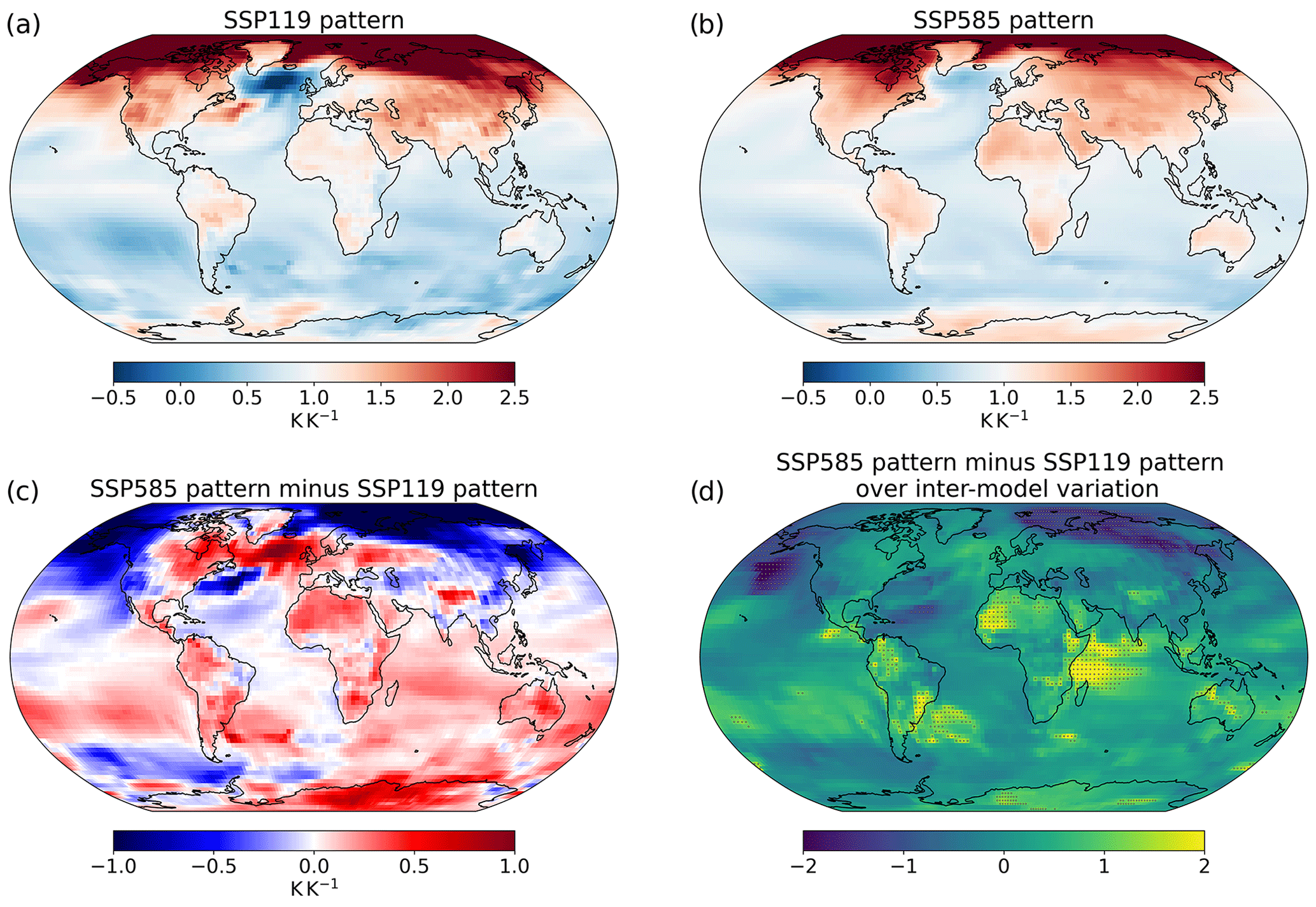
Figure 3 Mean warming patterns across eight ESMs derived from SSP1–1.9 (a) and SSP5–8.5 (b) simulations, the SSP5–8.5 minus that from SSP1–1.9 (c), and this difference divided by the inter-model standard deviation in this difference (d). Panel (d) shows stippling where the multi-model mean difference is greater than 1 inter-model standard deviation.

Figure 3 applies the same analysis to SSP1–1.9 and SSP5–8.5; the local temperatures are again regressed onto the global response to generate the response pattern. The SSP5–8.5-derived pattern shows greater sensitivity over land, consistent with the higher warming rate maintained through the century in this scenario, and a less sensitive Arctic, likely due to a saturation of the Arctic sea ice feedback (Huang et al., 2020; Lynch et al., 2017). Overall, the pattern difference is similar to the transient minus equilibrium patterns found in previous studies (Herger et al., 2015; Huang et al., 2020; King et al., 2020; Mitchell, 2003). This suggests that the difference between spatial patterns of warming in SSP1–1.9 and SSP5–8.5 may be driven primarily by the differences in disequilibrium rather than aerosol emissions; aerosols can be expected to play a relatively larger role in the pattern difference between scenarios closer in radiative forcing and/or with larger aerosol emissions differences. The lower temperature sensitivity in East Asia under SSP5–8.5 may be linked to the weaker reduction in aerosols there than in SSP1–1.9, resulting in less unmasking of the cooling effect. Some features of the SSP5–8.5–SSP1–1.9 pattern difference vary from the RCP8.5–RCP2.6 differences found by Ishizaki et al. (2012), who found a more sensitive Arctic under the higher-emissions scenario. This, they suggested, may be attributable to stronger ice melt overall under RCP8.5, due to thinning of the sea ice under warming. This highlights the contingency of the local sensitivity on the baseline climatology; further analysis of these background conditions in the ESMs may aid in explaining the differences (Lynch et al., 2017), but this is beyond the scope of this paper. Compared to Fig. 2, the pattern differences are typically smaller than those between hist–GHG and hist–aer, with most areas seeing differences of less than 0.3 K, consistent with differences between scenario patterns in prior studies (Huang et al., 2020; Ishizaki et al., 2012; Lynch et al., 2017; Mitchell et al., 1999; Mitchell, 2003).

Compared to the DAMIP comparison, the SSP1–1.9 and SSP5–8.5 pattern difference is not as robust between models (Fig. 3d compared to Fig. 2d), reflecting both a similarity between the scenario patterns and the extent of inter-model variation. This is expected, due to the narrower differences in forcers between scenarios, and is consistent with prior work on pattern differences between scenarios (Goodwin et al., 2020; Herger et al., 2015; Osborn et al., 2016, 2018; Tebaldi and Arblaster, 2014; Tebaldi and Knutti, 2018). Figure S2 shows the analysis for all the combinations of the five SSPs analysed in this study; generally, differences between SSPs closer in radiative forcing show fewer coherent differences in their spatial patterns, which is in agreement with Osborn et al. (2018).

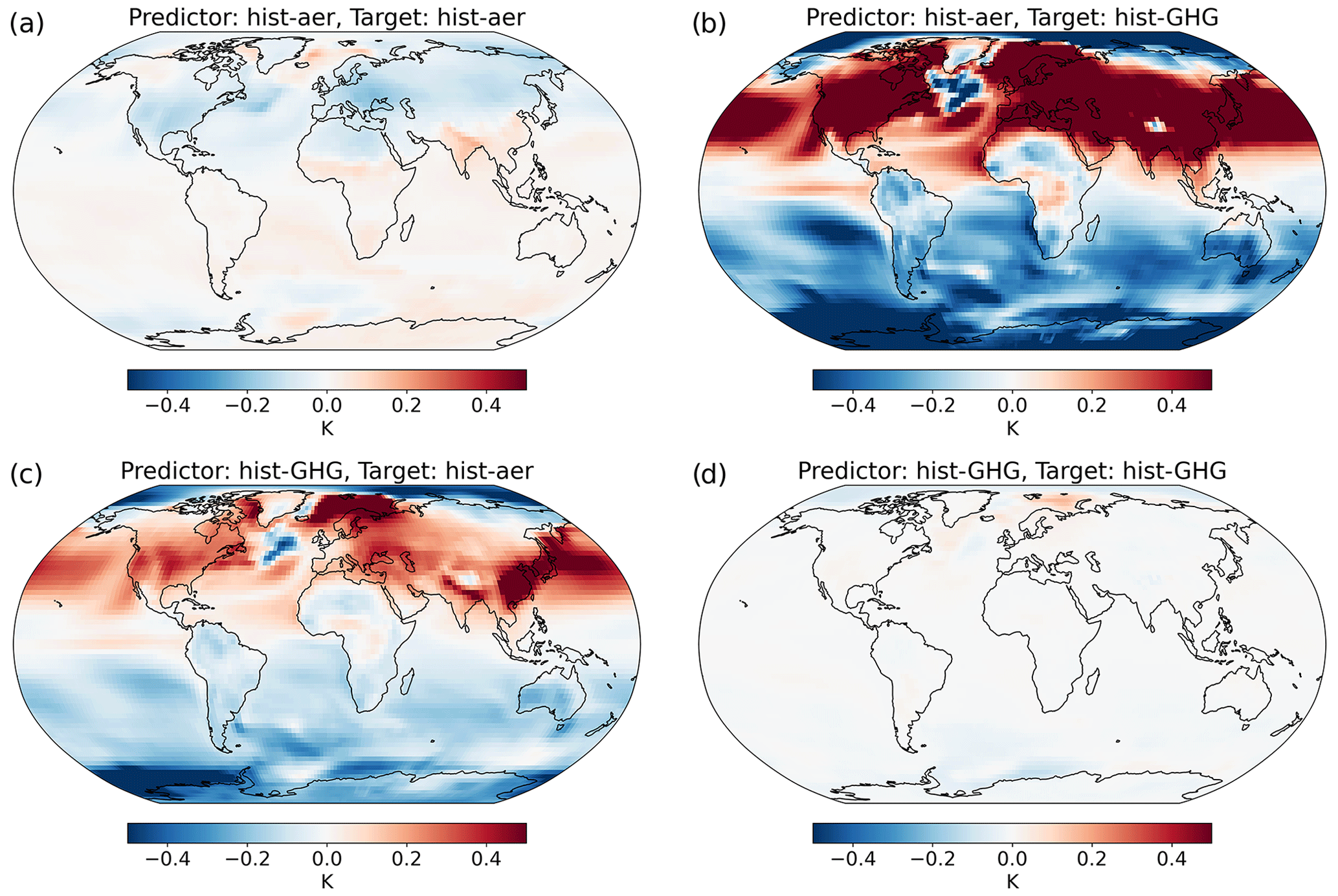
Figure 4 The 1990–2020 pattern scaling errors (emulation minus ESM) averaged across 10 ESMs when predicting with historical GHGs and aerosols separately and targeting the historical GHG and aerosol response separately; there are four combinations in total. The ESM and emulation data are taken relative to the first 50 years of the scenarios (i.e. 1850–1900). The last 30 years are shown to indicate the errors that arise once a substantial forcing has been applied and to study the self-emulation scaling error within the period, as self-emulation scaling errors cancel over the whole period.

Clear differences, which are larger over broad areas than the inter-model standard deviation, are therefore found between the temperature response patterns attributable to different historical forcers and consistent with their different spatial patterns. These differences are less systematic across ESMs for the future scenarios analysed, which are likely relatively more affected by their differing warming rates.

3.2 Total pattern scaling error

The total emulation error arising from the use of the two DAMIP-derived patterns (hist–aer and hist–GHG, Fig. 2) to separately emulate both DAMIP experiments are displayed in Fig. 4.

Out-of-sample errors are generally substantially larger than self-emulation ones (Osborn et al., 2018), since out-of-sample emulations introduce pattern errors in addition to the time series error. The out-of-sample emulations are too warm over the NHMLs and too cool in the Southern Hemisphere, in keeping with the pattern differences. In the hist–aer : hist–GHG emulation (using the hist–aer pattern to emulate the hist–GHG response; Fig. 4b), the warming in the NHMLs is overestimated, since the aerosol pattern is stronger here than the GHG response, and the Southern Ocean is conversely weaker, due to the historical spatial pattern of aerosol forcing. In the hist–GHG : hist–aer emulation, although the anomaly is positive over the NHMLs, this represents an underestimation of the cooling (since both the emulation and ESM data are negative). This is due to the relatively weaker GHG response here.

Variation in the local and global time series shapes can be due to spatial variations in the forcing or in the response. Self-emulation hist–GHG errors are small, indicating that there is little internal time series variation in this experiment. This is consistent with the well-mixed nature of GHGs. There will still be physical non-linearities, in both the concentration–forcing and forcing–response mechanisms, and internal variability, which are reflected in the non-zero self-emulation errors, but these are small in magnitude. The largest feature is an oversensitivity in the Arctic, which may be due to a saturation of the ice–albedo feedback.

In the hist–aer self-emulation, by comparison, while still small compared to the out-of-sample errors, some coherent errors occur. Negative anomalies (overestimated cooling) occur in the NHMLs, with positive ones (underestimated cooling) over the tropics and south Asia. This indicates that the sensitivity of the NHML temperature to the global change is lower in the period 1990–2020 than the average across the full time series, since the local parameters calculated across the entire time series are too strong at this time. This is consistent with a shift in aerosol emissions from the NHMLs to Asia over the last 3 decades and explains the positive anomalies over Asia; the emulation is undersensitive here in this period, since aerosol emissions are more concentrated in Asia in 1990–2020 than on average through the period. This is validated by Fig. S3, which shows the reverse effect in the mid-20th century (as NHML aerosol emissions were historically concentrated locally in this period) and the earlier peaking of NHML temperatures than the global average in hist–aer.

Pattern scaling errors in a given period can therefore be related to the differences in the average pattern between the predictor and target scenarios and the internal dynamics of the target scenario, particularly due to spatial variations in the forcing. Note that the time series self-emulation scaling error is also included in the total out-of-sample error, though the relative size indicates the pattern error is the dominant factor. These relative sizes are explored in more detail in Sect. 3.4.

The pattern scaling errors in Fig. 4 are typically less than 0.2 K for self-emulation and over 0.5 K for out-of-sample projection in the NHMLs. This out-of-sample error is substantial compared to the simulated temperature change of around 1.5 K $/$ −0.5 K globally in hist–GHG $/$ hist–aer and 2 K $/$ −1 K in the NHMLs. As for the pattern differences, these out-of-sample errors are larger than those typically found under pattern scaling (Alexeeff et al., 2018; Herger et al., 2015; Mitchell et al., 1999; Mitchell, 2003; Osborn et al., 2018; Tebaldi and Knutti, 2018), especially considering the magnitude of global warming in the scenarios, due to the starker differences between the forcing patterns in these idealised experiments. Since the out-of-sample pattern error scales with the pattern difference, Fig. 4b and c display very similar patterns, with the same sign of error over essentially all grid points (Fig. S4).

The errors in Fig. 4 divided by the inter-model standard deviation in the error are shown in Fig. S5. Errors are substantial in the out-of-sample emulations over both the NHMLs and the Southern Ocean, which is consistent with the large pattern differences in Fig. 2. The hist–GHG self-emulation shows no coherent errors, due to the lack of pattern error and coherent time series variation, but the NHML errors in the hist–aer self-emulation are consistent between the models, indicating agreement on the time series error found here.

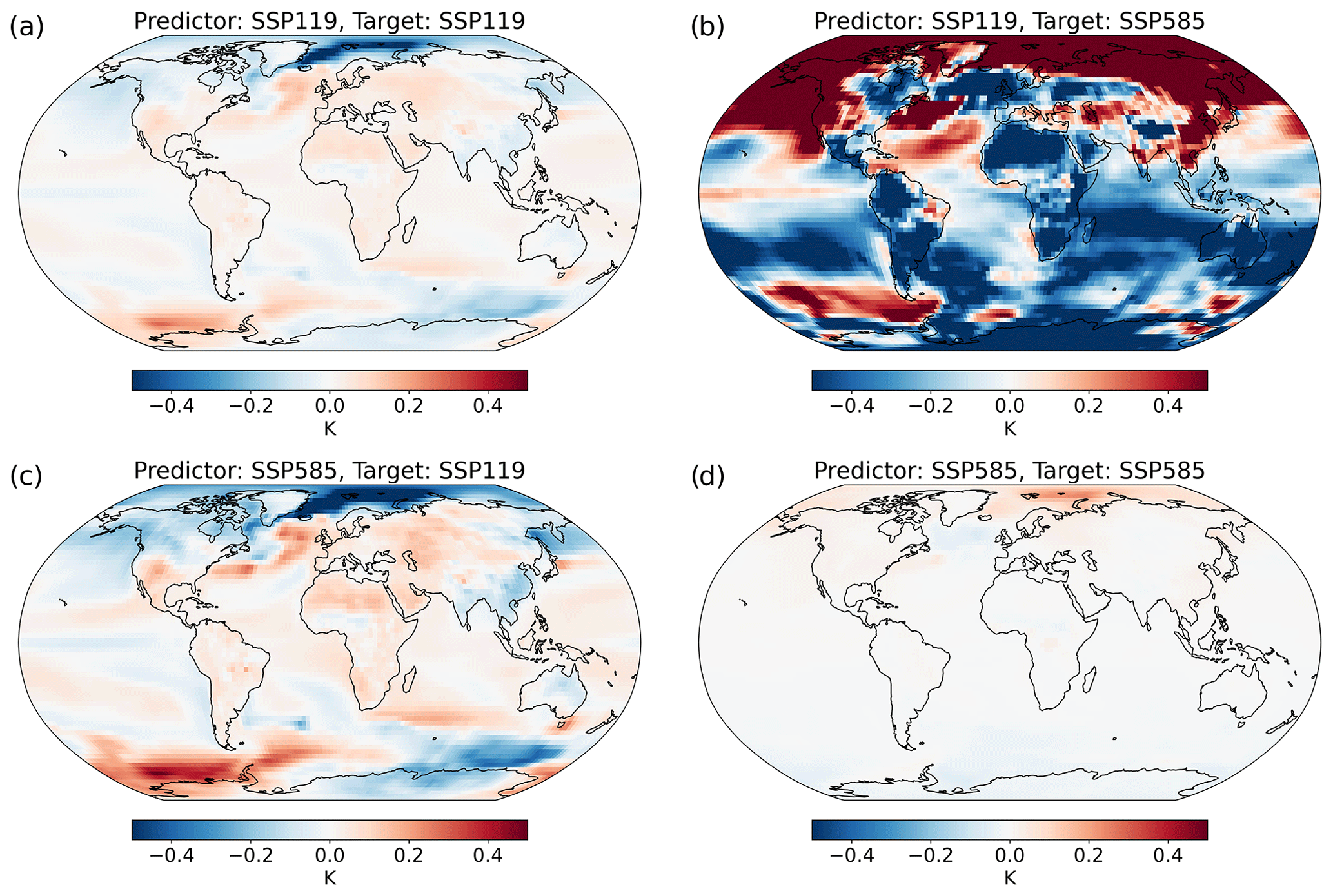
Figure 5 The 2070–2100 pattern scaling errors (emulation minus ESM) averaged across eight ESMs when predicting with SSP1–1.9 and SSP5–8.5 separately, and targeting the SSP1–1.9 and SSP5–8.5 responses separately; four combinations in total. The ESM and emulation data are taken relative to the first 50 years of the scenarios (i.e. 2015–2065).

Similarly, Fig. 5 shows the 2070–2100 multi-model mean pattern scaling errors under the four combinations of the SSP1–1.9 and SSP5–8.5 scenarios (self-emulation and cross emulation), and Fig. S6 shows these divided by the inter-model standard deviation. The out-of-sample errors are again larger than those attributable to self-emulation alone, indicating a substantial role of the pattern difference. They are consistent with the pattern differences in Fig. 3. However, similar to the pattern differences, the inter-model standard deviation is generally larger than the magnitude, with errors greater than the inter-model standard deviation generally only in areas with similarly large difference in the patterns themselves. The time series (self-emulation) error is small in SSP5–8.5, similar to hist–GHG, but SSP1–1.9 shows larger errors, with a pattern consistent with the pattern differences. This time series error, as with hist–aer, must be driven by the internal characteristics of SSP1–1.9. The period 2070–2100 exhibits weaker positive warming trends than the time series average, with peak warming occurring in mid-century on average. Thus, the parameters derived from the time series average will be too sensitive over land and tropical oceans, as the climate is experiencing less positive forcing than average, similar to the SSP5–8.5–SSP1–1.9 pattern difference. This leads here to broad, coherent self-emulation scaling errors over 2070–2100, but as for the out-of-sample cases, there is little inter-model agreement. Consistent results are found for each pair of the five SSPs used here, as shown in Figs. S7 and S8; extrapolation to project higher forcing scenarios using lower forcing patterns is found to introduce substantial errors, with interpolation to lower forcing scenarios generating smaller errors, although still larger than self-emulation due to the additional effect of pattern errors (Herger et al., 2015; Mitchell, 2003; Tebaldi et al., 2020). The errors are typically less than 0.3 K under self-emulation, remaining less than 0.5 K under strong interpolation, but are over 0.5 K in broad areas under strong interpolation. This compares to around 1.4 K (4.4 K) warming relative to preindustrial times in SSP1–1.9 (SSP5–8.5) over 2081–2100 (IPCC, 2021). These self-emulation and interpolation errors are consistent with those found in prior work (Alexeeff et al., 2018; Herger et al., 2015; Mitchell et al., 1999; Mitchell, 2003; Osborn et al., 2018; Tebaldi and Knutti, 2018), while the extrapolation errors are larger due to the extreme case study presented in this section.

3.3 Relative importance of the pattern and time series errors

As highlighted above, it is important to understand how the magnitude and relative size of the two types of pattern scaling error – pattern and time series – depend on the target and predictor dataset.

Pairwise predictor–target emulations are performed for the 25 combinations of the five SSPs analysed here. Maps of the time series and pattern errors are both calculated in each year of each simulation. Pattern scaling errors are zero on the global average by design, as the pattern is scaled by the global mean response; so, to analyse the size of the errors, the global average of the absolute error magnitude is taken for each. The magnitude of the total error is also taken; this is equal to the time series error for self-emulation, but for out-of-sample emulations, local cancellations from opposite-sign time series and pattern errors cause this total error to be less than the sum of the two. This sum of the two – termed the sum error – is also calculated to allow for comparisons between the two magnitudes.

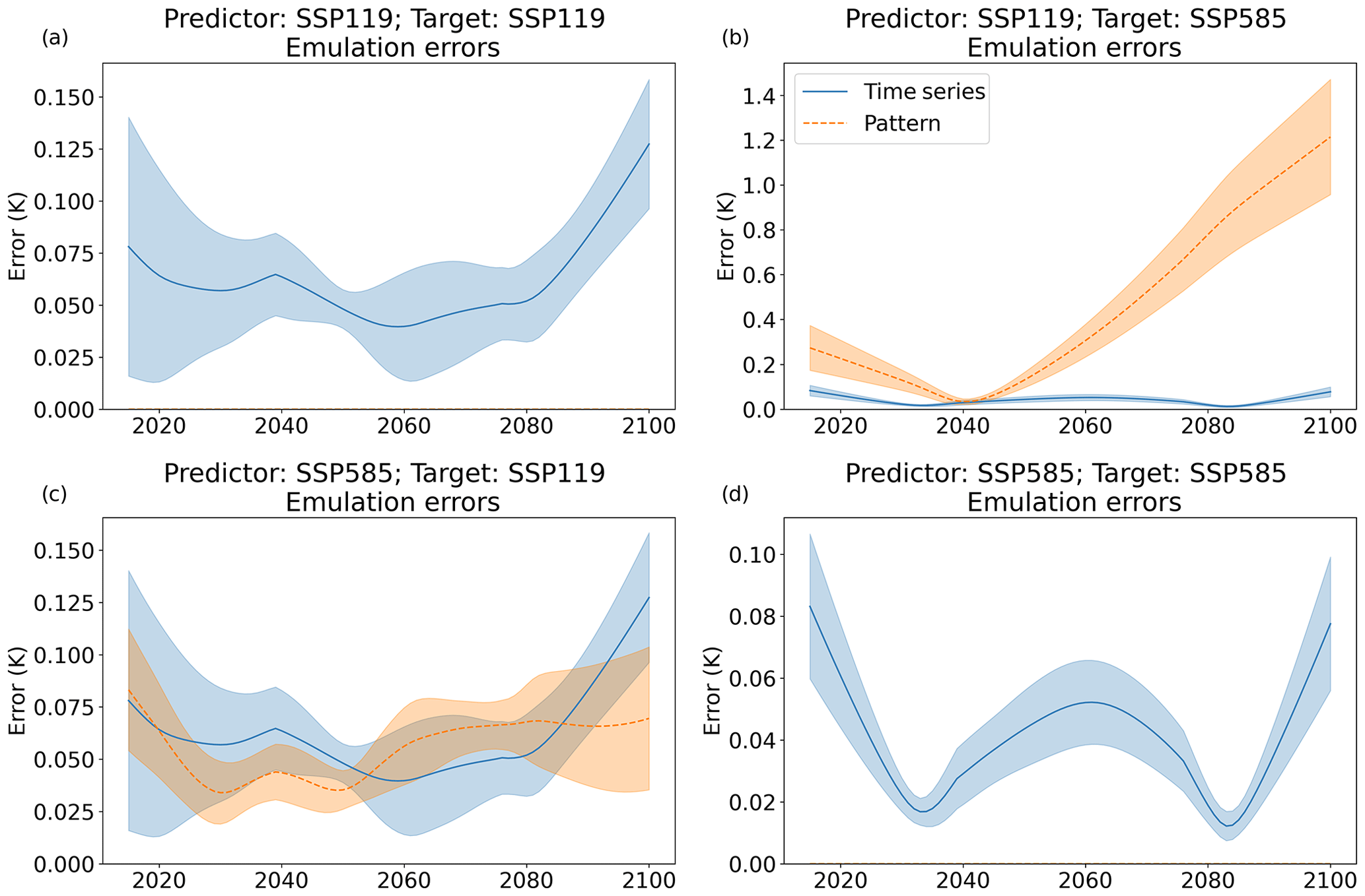
Figure 6 Time series of the size of the global average pattern scaling error attributed to pattern errors and time series errors. Each line gives the multi-model mean, with shading indicating plus and minus 1 inter-model standard deviation. Note the varying vertical scales.

Figure 6 shows the 2015–2100 time series of the pattern and time series errors for the four combinations of SSP1–1.9 and SSP5–8.5. Figure S9 gives the results for each of the 25 SSP combinations, with a fixed scale.

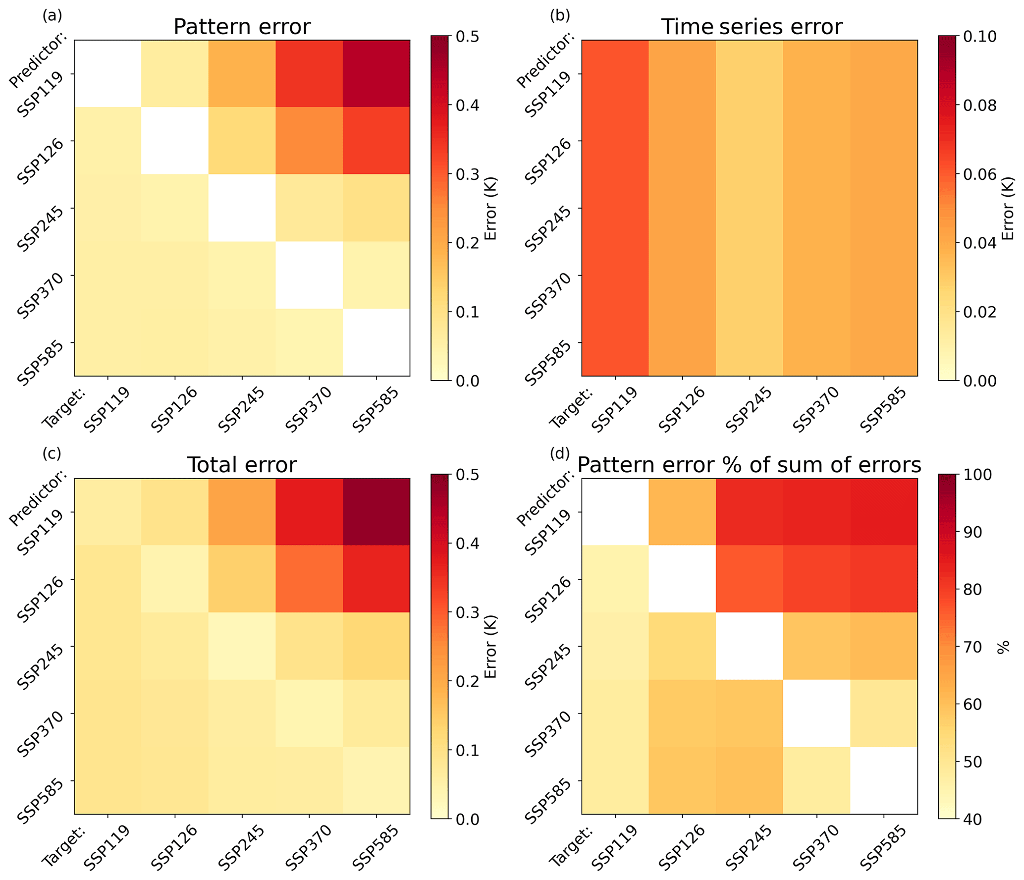
Figure 7 Pattern scaling errors averaged over the scenario time period for each predictor–target pair. Errors are calculated annually and then the absolute value is taken and averaged across time and models. (a) The pattern error, (b) The time series error (with a smaller scale). (c) The total error. Panel (d) gives the percentage of the absolute total error (the sum of pattern and time series) attributed to the pattern error. Note the smaller scale on the time series error plot.

The time series error, dependent only on the target scenario, varies relatively little between scenarios, while the pattern error is substantially larger for extrapolation cases. Even for adjacent extrapolation – e.g. using SSP1–2.6 to emulate SSP2–4.5 – the pattern error becomes increasingly large by 2100.

The magnitude of the time-averaged pattern, time series, and total errors in each pair is shown in Fig. 7 for the 25 scenario combinations, along with the percentage of the sum error (the sum of the magnitudes of each component) given by the pattern error. The sum of the error magnitudes is used for comparison, as opposing-sign errors will partially cancel out in the total. The magnitude of the time series error is less than 0.1 K in all scenarios but the largest in SSP1–1.9, a scenario in which this error can represent a substantial fraction of the mean response. The pattern error, which is zero for self-emulation by definition, is systematically greater for extrapolation, likely strongly influenced by the scaling of the pattern difference by the target scenario global mean time series. Global and time-averaged pattern error magnitudes can reach almost 0.5 K under the highest extrapolation (SSP1–1.9 : SSP5–8.5) but are still around 0.2 K for slighter extrapolations and 0.1 K under interpolation. The total error is therefore the highest for extrapolation. There is less dependence of the total error on the predictor scenario when targeting a low-emissions scenario than targeting a high one, due to the greater role of the time series error. Note the small variations in the SSP1–1.9 column compared to the SSP5–8.5 one.

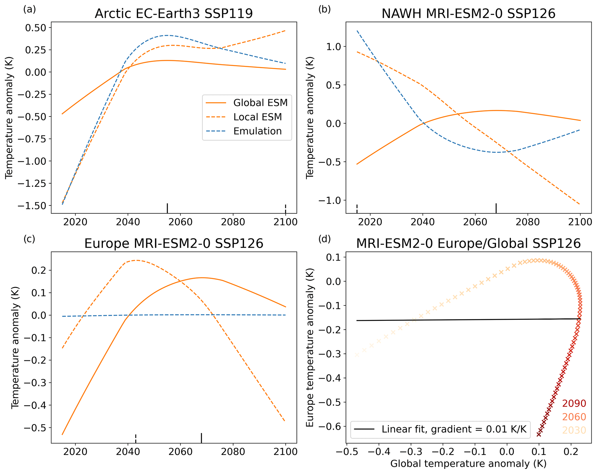
Figure 8 Time series of global and regional ESM annual temperature changes (relative to the first 50 years of a scenario), with both annual and LOWESS values smoothed, and the projected regional emulation from fitting a linear regression to the local and global smoothed temperatures for three region–model–scenarios, namely the Arctic (60 to 90^∘ N) in EC-Earth3 under SSP1–1.9 and the North Atlantic (40 to 50^∘ N, 40 to 20^∘ W) and Europe (35 to 70^∘ N, 10^∘ W to 40^∘ E) in MRI-ESM2-0 in SSP1–2.6. Perfect emulation would occur if the dashed orange lines and dashed blue lines – the local ESM data and the local emulation – overlapped; deviations from this are the pattern scaling error. The local and global peak warming years are indicated with short dashed and solid vertical black lines, respectively, which project from the time axis. Also shown is the regression curve for the third example (d).

Pattern errors represent a different proportion of the sum of errors under different pairs, accounting for over 80 % under high extrapolation but only around half for projecting SSP1–1.9. The intrinsic time series error, irreducible under this methodology, accounts for a much larger fraction of the error under low-emissions scenarios than the pattern error. This larger role of the time series error is consistent with the lower correlation between local and global temperatures under low-emissions scenarios found by Lynch et al. (2017).

3.4 Effect of peak warming on time series error

The year of peak warming is increasingly used to classify emissions scenarios (Riahi et al., 2022). One implication of simple pattern scaling approaches tied to global warming level is that if, in a low-emissions scenario, the global warming time series peaks in a particular year, then by construction the emulated temperature peaks in this same year in every grid point. The spatial pattern of this peak warming year is then homogeneous by design. Any spatial structure in the peak warming pattern of the actual ESM target data will be missed, leading to pattern scaling errors.

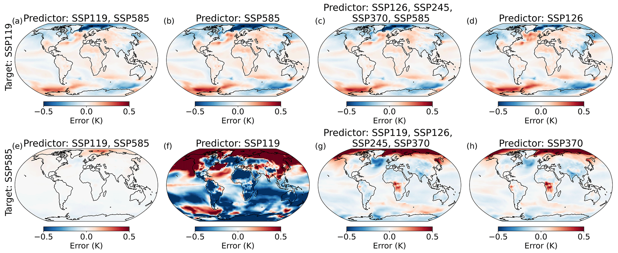
Figure 9 The 2070–2100 pattern scaling errors when projecting SSP1–1.9 (a–d) and SSP5–8.5 (e–h) for patterns using the following four sets of predictors: envelope (a, e; SSP1–1.9 and SSP5–8.5), opposite (b, f; SSP5–8.5 for targeting SSP1–1.9 and vice versa), all others (c, g; i.e. the four scenarios other than that being targeted), and nearest (d, h; SSP1–2.6 to target SSP1–1.9 and SSP3–7.0 to target SSP5–8.5 – the nearest scenario to each target in radiative forcing terms). The patterns are calculated via the regression of local on global temperatures, as described in Sect. 2.2, and the ESM and emulated data are also baselined to the first 50 years of the scenario (i.e. 2015–2065).

The effect of this can be tested by exploring the peak warming simulated in ESM simulations of low-emissions scenarios. Figure S10 shows the multi-model mean of the deviation in the local year of peak warming from the global average, along with the magnitude of this deviation minus the inter-model standard deviation, for both SSP1–1.9 and SSP1–2.6. The local year of peak warming is shown for each model and the multi-model mean in Fig. S11. Generally, tropical land and oceans peak earlier than average, and the Arctic and Southern Ocean later, which is consistent with the inertia of the system (as seen in Fig. 3). The patterns are similar between SSP1–1.9 and SSP1–2.6, indicating some consistency between scenarios in this effect. Few areas see inter-model agreement, however, with agreement on earlier peaking over some tropical oceans and land and later peaking over the east of the Southern Ocean. By 2100, higher forcing scenarios are typically still warming everywhere, except for some models that show a pronounced North Atlantic warming hole (NAWH), which is the area of the North Atlantic where the general warming has been masked by circulation-change-induced local cooling historically (Huang et al., 2020) (not shown).

Figure 8 shows results from three region–model–scenario combinations, which have been chosen to demonstrate the different effects this can have on emulation errors. In the Arctic in EC-Earth3 under SSP1–1.9 case (Fig. 8a), the ESM global temperature peaks in the mid-century, but the Arctic continues to warm to 2100. Since the pattern scaling projection is simply scaled by the global mean, however, the Arctic emulation peaks with the global temperature, diverging from the ESM to the end of the century and projecting the wrong sign of trend from the mid-century onwards.

Figure 8b applies this to the NAWH in MRI-ESM2-0 under SSP1–2.6. In the ESM, the NAWH cools throughout the century, while global temperatures peak around 2070. The pattern scaling parameter here is negative, as local cooling is regressed onto overall global warming. The projected NAWH response therefore reaches a minimum when the global mean peaks and warms from there to 2100 as global temperatures reduce.

Finally, Fig. 8c applies this to Europe in MRI-ESM2-0 under SSP1–2.6. In the ESM data, European and global temperatures rise, stabilise, and fall, but as a land region near the NAWH, Europe peaks in temperature several decades before the global mean. As shown in Fig. 8d, these different regional and global shapes happen to produce a linear fit with almost exactly zero gradient. Although Europe sees substantial temperature change through the century, the sensitivity averages to zero due to the differing global peak time. The resultant emulation thus has essentially zero amplitude, deviating strongly from the substantial changes modelled over Europe in the ESM.

4 Implications for the use of pattern scaling

In this section, the implications of the prior findings for the application of pattern scaling are investigated. When emulating a given scenario, a choice must be made for the predictor dataset, i.e. the scenario(s) used to generate the pattern. The effect of this choice on pattern scaling errors is important; it will not affect the time series error by definition but will modify the pattern error and hence the overall emulation efficacy. Four options are studied here to target both SSP1–1.9 and SSP5–8.5 separately; some include the target scenario in the predictor dataset, thus not being entirely out-of-sample, but multiple predictor scenarios are used in these cases, thus not being purely self-emulation. The “envelope” option uses both SSP1–1.9 and SSP5–8.5 to construct a pattern using information from the extremes of the available dataset. The “furthest” option uses the most different scenario – SSP5–8.5 to emulate SSP1–1.9, and vice versa. This is an unlikely choice but is a test that can give information about the effect of a wide range of choices. The “all others” category utilises all of the available scenarios except the target one, and “nearest” uses the closest scenario in nominal 2100 radiative forcing. The 2070–2100 multi-model mean errors associated with these eight cases are shown in Fig. 9; the errors divided by the inter-model standard deviation are shown in Fig. S12.

The SSP1–1.9 error maps are remarkably insensitive to the choice of predictor datasets; the time series error intrinsic to SSP1–1.9, a substantial fraction of the error as shown in Fig. 7, ensures a baseline error. Since the disequilibrium is qualitatively similar between early–late SSP1–1.9 (responsible for the time series error) and other scenarios in SSP1–1.9 (giving the pattern error), the distributions of the pattern and time series errors are similar. When targeting SSP5–8.5, however, a clear difference in the error magnitude is found when using different predictor datasets. Low errors occur with the envelope method, with similarities seen in the self-emulation pattern, suggesting that SSP5–8.5 drives the pattern generated from the combination. The furthest case gives large errors as expected; all others and nearest give relatively similar, and smaller, errors.

The patterns of comparison between the error magnitude and the inter-model deviation (Fig. S12) are very similar, with few areas of agreement between models. This is unsurprising for SSP1–1.9, given the similarity of the error, but for SSP5–8.5, the substantially different error magnitudes and patterns result in similar, and small, areas of agreement in the pattern scaling error. This is presumably because the inter-model spread scales with the magnitude of the error, reflecting disagreement in the driving processes of the pattern scaling errors. This is again consistent with prior findings that inter-model variation is larger than pattern scaling errors (Goodwin et al., 2020; Herger et al., 2015; Osborn et al., 2016, 2018; Tebaldi and Arblaster, 2014; Tebaldi and Knutti, 2018).

5 Discussion and conclusions

This study presents a decomposition of pattern scaling errors into two components, namely one due to differences in the pattern between the predictor and target datasets (the pattern error) and one due to internal non-linearities in the target scenario (the time series error). The differences in warming patterns between pairs of single-forcer experiments and plausible future scenarios causing the pattern error were also investigated, along with case studies of the impact of the time series error, and the total impact on the application of pattern scaling to the SSPs was tested. In each case, pattern scaling was applied to individual models, with the pattern scaling error for each model calculated as the difference between the ESM data and the model-specific emulation.

Self-emulation uses the correct pattern – i.e. that of the scenario being emulated – and is conceptualised to therefore have zero pattern error. Errors then occur due to differences in the temporal shape of the local and global temperature. These differences are intrinsic to the scenario and are irreducible under simple pattern scaling. Here, spatial differences in the peak warming year in low-emissions pathways were found to manifest in substantial emulation errors across regions and models.

When emulating out of sample, pattern errors are introduced due to the pattern differences between the scenarios, thereby combining with the time series error in the target scenario. Robust differences were found between temperature change patterns under historical GHG and aerosol forcings, with the NHMLs more sensitive under aerosol forcing due to the historical predominance of aerosol emissions there. Differences between temperature change patterns under future scenarios were less clear between models, as found in prior work studying future emissions scenarios (Goodwin et al., 2020; Herger et al., 2015; Osborn et al., 2016, 2018; Tebaldi and Arblaster, 2014; Tebaldi and Knutti, 2018). However, the difference resembled differences between transient and equilibrium patterns in prior work (Herger et al., 2015; Huang et al., 2020; King et al., 2020; Mitchell, 2003), with higher sensitivity over tropical land and lower over high-latitude oceans in SSP5–8.5, thus indicating that the different warming rates in the scenarios are an important cause of difference between these scenario patterns. Aerosol concentrations are also substantially different between these scenarios, potentially causing a less-sensitive East Asian response under SSP5–8.5, though this was not robust between models.

The pattern error drives over 80 % of the overall pattern scaling error when emulating a high-emissions scenario using a low-emissions pattern, causing pattern scaling errors to be strongly dependent on the predictor dataset used. In contrast, the time series error contributes around half of the error for emulating low-emissions scenarios, rendering the choice of pattern less important, though choosing scenarios closer in radiative forcing to the target still reduces the overall error.

Splitting the total error into these components allows for an understanding of the relative importance of the limitations of the assumptions which generate the errors. Understanding which source drives the error for a given pattern scaling application can guide efforts to reduce these uncertainties.

The errors associated with differing aerosol emissions and differing levels of warming, including stabilisation and relative cooling, will presumably be more important for the SSPs analysed here than the prior RCPs, which saw a narrower range in aerosol emissions and levels of warming. The tighter range in CO₂ and non-CO₂ forcings ensured that pattern scaling worked well under the RCPs (Goodwin et al., 2020), but variations in the aerosol pattern will lead to greater pattern scaling errors (Xu and Lin, 2017). Projecting existing and future Paris-Agreement-consistent scenarios, i.e. those which stabilise temperatures below 2 ^∘C and reach net-zero GHG emissions by 2100 (Schleussner et al., 2022), such as the C1 and C2 scenarios in IPCC AR6 WGIII (Kikstra et al., 2022), will lead to issues related to equilibrium and transient pattern differences (King et al., 2020).

The efficacy of pattern scaling is constrained by the choices of patterns available, i.e. the dataset of scenarios simulated in multi-model ESM ensembles, which is itself determined by the trajectories chosen under projects such as ScenarioMIP. These might not cover the full relevant range of scenario attributes (Guivarch et al., 2022); there is a lack of stabilising and cooling scenarios in the extant datasets (Tebaldi et al., 2022), with a recognised need for more equilibrium experiments in the future (King et al., 2021). However, this work demonstrates that scenarios with these properties are less amenable to emulation via pattern scaling than higher-emissions ones.

These results suggest that caution should be taken when applying simple linear pattern scaling to emulate low-emissions scenarios, as these are intrinsically less amenable to emulation via pattern scaling. Large differences in the forcing pattern and rate of warming between predictor and target scenarios also lead to substantial emulation errors.

This paper focused on annual mean temperature, but it would be useful to determine the relative roles of the pattern and time series errors for other variables in order to determine the extent to which their emulation is limited by non-linearities in the target scenario. The distribution of temperature variability is also crucial for impact analysis, as it can change under external forcing (Olonscheck and Notz, 2017; Pendergrass et al., 2017) and has been incorporated into emulation tools such as MESMER (Beusch et al., 2020).

Only simple pattern scaling – using one predictor, global temperature, to emulate the local temperature response using a single pattern – was studied here. These errors may be mitigated to an extent by other methods, such as using patterns dependent on a forcer (Xu and Lin, 2017; Kravitz et al., 2017; Schlesinger et al., 2000) or response timescale (Zappa et al., 2020). Improvements have also been found by adding extra predictors in addition to global temperature, such as land–sea contrast (Herger et al., 2015) and ocean heat uptake (Beusch et al., 2020). The pattern generated across a given ensemble may depend on the number of members, with greater internal variability for smaller ensembles. Most ensembles used here were larger than three, but several ensembles had only one member (Tables S1 and S2). The extent to which this ensemble size affects the pattern is uncertain and is an avenue for future work.

Regional climate changes are key for understanding the impacts of different policy choices, but the links between global mean temperatures and their regional impacts have not been fully explored within the IPCC framework (Kikstra et al., 2022). Emulation of regional impacts via tools such as pattern scaling, in a consistent framework such as MESMER (Beusch et al., 2020), provides a crucial means by which to estimate the local impacts of new emissions scenarios without the need to perform expensive, time-consuming ESM simulations.

This paper furthers the understanding of pattern scaling by decomposing the errors into those that are attributable to different assumptions. Further research to reduce these errors where possible will be crucial to enhance our understanding of future climate change.