Past and future response of the North Atlantic warming hole to anthropogenic forcing

Most of the North Atlantic ocean has warmed over the last decades, except a region located over the subpolar gyre, known as the North Atlantic “warming hole” (WH), where sea surface temperature (SST) has in contrast decreased. Previous assessments have attributed part of this cooling to the anthropogenic forcings (ANT) – aerosols (AER) and greenhouse gases (GHGs) – modulated by decadal internal variability. Here, I use an innovative and proven statistical method which combines climate models and observations to confirm the anthropogenic role in the cooling of the warming hole. The impact of the aerosols is an increase in SST which is opposed to the effect of GHGs. The latter largely contribute to the cooling of the warming hole over the historical period. Yet, large uncertainties remain in the quantification of the impact of each anthropogenic forcing. The statistical method is able to reduce the model uncertainty in SST over the warming hole, both over the historical and future periods with a decrease of 65 % in the short term and up to 50 % in the long term. A model evaluation validates the reliability of the obtained projections. In particular, the projections associated with a strong temperature increase over the warming hole are now excluded from the likely range obtained after applying the method.

1 Introduction

The increase of global surface air temperature (GSAT) over the 1850–2021 period is unequivocally attributed to human activities (Lee et al., 2021). This increase is spatially heterogeneous, with some regions warming less rapidly than others, or even cooling. Noticeably, sea surface temperature (SST) over the so-called North Atlantic “warming hole” (hereafter WH) region, which is located over the subpolar gyre, has decreased over the 1901–2021 period relative to the 1870–1900 period (Gutiérrez et al., 2021). This long-term decrease is often associated with modifications in the meridional transport of oceanic heat content in the North Atlantic (Gervais et al., 2018; Hu and Fedorov, 2020) and with a slowing down of the Atlantic Meridional Overturning Circulation (AMOC) (Rahmstorf et al., 2015; Caesar et al., 2018). Melting of the Arctic sea ice and the Greenland ice cap may have contributed to this cooling (Allan and Allan, 2019; Gervais et al., 2018; Keil et al., 2020; Liu et al., 2019), but atmospheric processes have also been proposed (Li et al., 2022; Keil et al., 2020). Although internal variability strongly influences interannual to decadal variability in the North Atlantic SST (Robson et al., 2016; Hodson et al., 2014; Moffa-Sánchez et al., 2019), several detection and attribution studies indicate a contribution of anthropogenic greenhouse gases (GHGs) to explain the long-term cooling of the WH over the historical period (Chemke et al., 2020; Dagan et al., 2020). Concomitantly, natural and especially anthropogenic aerosols (AER) may have played a role in shaping the temporal evolution of the SST over this region (Booth et al., 2012; Fiedler and Putrasahan, 2021) by delaying the cooling of the WH through an acceleration of the AMOC leading to a warming of the subpolar region (Dagan et al., 2020; Menary et al., 2020). Climate projections from both the fifth and sixth Coupled Model Intercomparison Projects (CMIP5 and CMIP6; Eyring et al., 2016) corroborate the contribution of GHGs, with some models projecting an enhanced cooling of the WH (Dagan et al., 2020; Sigmond et al., 2020; Marshall et al., 2015) but with large uncertainties in the spatiotemporal structure and intensity of the cooling (Menary and Wood, 2018; Bellomo et al., 2021). Given the potential impact of the North Atlantic SSTs on the Northern Hemisphere climate (Qasmi et al., 2021; Ren and Liu, 2021; Gervais et al., 2019, 2020; Karnauskas et al., 2021), it is important to investigate the extent to which it is possible to reduce the uncertainty in the SST projections over the WH.

So far, the impact of external forcings and internal variability on the observed WH over the historical period has been qualitatively estimated by using dedicated sensitivity model experiments (Sigmond et al., 2020) or initial-condition large ensembles (Dagan et al., 2020). Regardless of the various mechanisms that have been suggested to explain the WH, few studies have attempted to quantify in a strictly statistical sense the anthropogenic contribution to changes in SST over the historical period over this region. A recent detection and attribution study based on a statistical method derived from optimal fingerprinting provides a quantitative statement regarding an anthropogenic signal in the SST time series over the WH (Chemke et al., 2020) but without quantifying the influence of each external forcing. In this paper, I estimate (i) the contribution of each of the main external forcings in the evolution of the observed WH over the historical period, and (ii) the uncertainty on the evolution of the SST response to external forcings (hereafter forced response) over both the historical and future periods. These estimates come from the Kriging for Climate Change (KCC) method, an innovative and proven statistical method, which interpolates (hence the name kriging) observations and climate models. These different estimates are not based on any mechanistic assumptions or physical processes but are based solely on the SST averaged over the WH.

2 Data and methods

2.1 Observations

The SST observations from the HadSST4 (Hadley Centre's sea surface temperature, version 4) dataset (Kennedy et al., 2019) are used. These observations have the advantage of providing an estimate of the measurement uncertainty, which encompasses the treatment of incomplete data coverage, homogenization uncertainty, etc. through an ensemble of 200 equiprobable realizations over the 1870–2021 period. Compared to other datasets, this ensemble allows a more comprehensive estimation of the measurement error with the possibility of calculating the temporal covariance of uncertainty with the 200 members. Note that I do not consider other datasets because they usually fall within the uncertainty of HadSST4. The median of the 200-member ensemble will be considered as the best estimate, while all realizations are used to estimate the measurement uncertainty. Observations of global surface air temperature (GSAT) used by the KCC method are taken from the HadCRUT5 (Hadley Centre/Climatic Research Unit global surface temperature anomalies, version 5) ensemble of 200 members (Morice et al., 2021).

2.2 Climate models

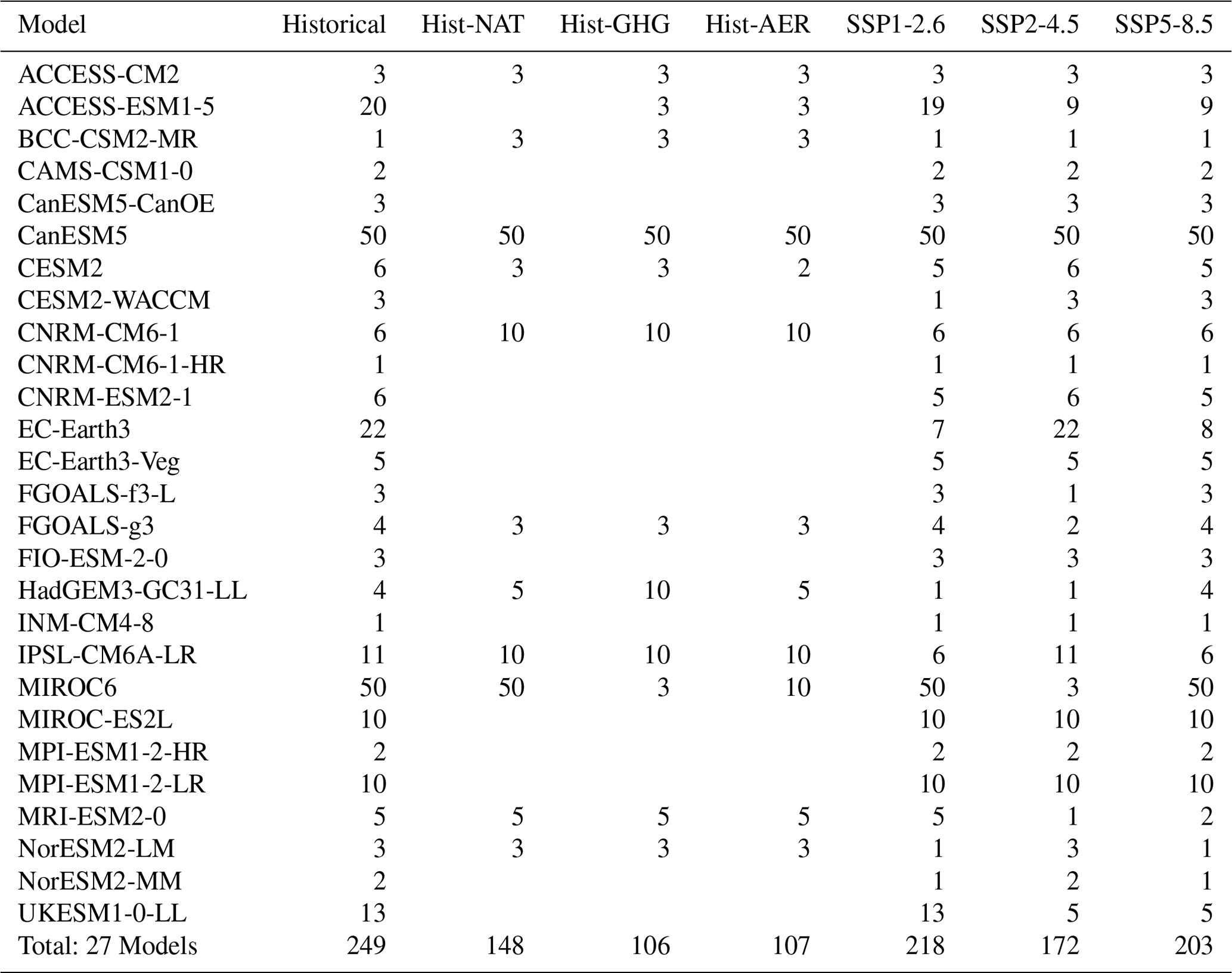
Historical and Scenario Model Intercomparison Project (ScenarioMIP) simulations from the CMIP6 ensemble (Eyring et al., 2016; O'Neill et al., 2016) are used to estimate the forced response of temperature to all external forcings (ALL) over the 1850–2100 period (the three scenarios – SSP1-2.6, SSP2-4.5 and SSP5-8.5 – are used). The contribution of each external forcing during the 1850–2020 period is estimated from the Detection and Attribution Model Intercomparison Project (DAMIP) ensemble (Gillett et al., 2016), especially from the hist-GHG and hist-AER simulations, in which GHGs and AER follow their historical concentrations, respectively, while other forcings are kept constant. The list of the models, the simulations used, and the number of members is provided in Table A1 in the Appendix. A particular feature of some of the CMIP6 models, on which the sixth assessment report (AR6) from the IPCC is based, is their high equilibrium climate sensitivities (ECS) (Lee et al., 2021). In the AR6, ECS and GSAT projections from the CMIP6 ensemble have been assessed by using statistical methods (including the one used in this study) and observations to provide GSAT estimates consistent with the observational record (Ribes et al., 2021). The statistical method used here takes these likely estimates of the results of ECS and GSAT future ranges into account, by including an observational constraint based on both GSAT and SST over the WH region.

2.3 Statististical method

To assess past and future forced response of the WH, I use the KCC observational constraint method that has been previously applied to global mean warming (Ribes et al., 2021) and regional warming (Qasmi and Ribes, 2022; Ribes et al., 2022). This technique works in three steps. First, the forced response of each climate model is estimated over the historical period. In order to also get attribution statements, the responses to ALL (all external forcings), NAT (natural forcings only) and anthropogenic GHG forcings are estimated separately. Second, the sample (or the probability distribution) of the forced responses from the CMIP6 models is used as a prior of the real-world forced response. This is done assuming that “models are statistically indistinguishable from the truth”. Third, observations are used to derive a posterior distribution of the past and future forced response in a Bayesian way. The procedure can be summarized using the following equations:

$$\begin{array}{}\text{(1)}& \mathit{y}=\mathbf{H}\mathit{x}+\mathit{ϵ},\end{array}$$

where y is the time series of observations (a vector) over the observed period, x is the time series of the forced response (a vector) over the historical and projected periods, H is an observational operator (matrix), ϵ is the random noise associated with internal variability and measurement errors (a vector), and $\mathit{ϵ}\sim \mathcal{N}(\mathrm{0},{\mathbf{\Sigma }}_y)$, where 𝒩 stands for the multivariate Gaussian distribution. The observational operator H is a matrix which extracts the components of x that are observed in y, thus all H coefficients are equal to 0 or 1 (see Eq. B1 and Appendix B). Climate models are used to construct a prior on $\mathit{x}:\mathrm{\Pi }\left(\mathit{x}\right)=\mathcal{N}({\mathit{\mu }}_x,{\mathbf{\Sigma }}_x)$. Then the posterior distribution for given observations y can be derived as $p\left(\mathit{x}\right|\mathit{y})=\mathcal{N}({\mathit{\mu }}_{\mathrm{p}},{\mathbf{\Sigma }}_{\mathrm{p}})$. In the following, I am interested in assessing the forced response of annual mean SST over the WH (projections) as well as the annual mean response to specific subsets of forcings (attribution) over the historical period. These forced responses could be constrained by various observations. Here, I consider constraints by both GSAT observations and regional annual mean SST averaged over the WH – the rationale behind this choice is discussed below. Therefore,

$$\begin{array}{}\text{(2)}& \mathit{x}=({\mathit{T}}_{\mathrm{glo}}^{\mathrm{all}},{\mathit{T}}_{\mathrm{reg}}^{\mathrm{all}},{\mathit{T}}_{\mathrm{reg}}^{\mathrm{ghg}},{\mathit{T}}_{\mathrm{reg}}^{\mathrm{nat}}),\end{array}$$

where each element is the annual forced response over the 1850–2100 period (except ${\mathit{T}}_{\text{reg}}^{\text{ghg}}$ which only covers 1850–2020); T stands for temperature; “all”, “ghg” or “nat” are the subsets of external forcings considered; “glo” and “reg” refer to GSAT and regional SST, respectively. The length of x is thus n_x=924. Similarly,

$$\begin{array}{}\text{(3)}& \mathit{y}=({\mathit{T}}_{\mathrm{glo}}^{\mathrm{obs}},{\mathit{T}}_{\mathrm{reg}}^{\mathrm{obs}}),\end{array}$$

i.e., only observed time series are used in y. The length of these time series varies: 1850–2021 for GSAT, 1870–2021 for the regional SST. As a result, y has a length of n_y=322. All attribution or projection diagnoses presented below can be derived from the posterior distribution p(x|y). Accounting for GSAT is important because various recent studies argued that the observational constraint on this variable is robust (e.g., to the choice of the statistical method), with the high end of simulated GSAT model responses not consistent with observed GSAT changes (Lee et al., 2021, and references therein). As there is some dependence (between CMIP models) between future GSAT changes and regional changes over most regions including the WH, a reduced GSAT response is expected to imply a reduced regional warming. This is confirmed by Qasmi and Ribes (2022), who found that accounting for the global constraint clearly improves the accuracy of regional projections. Accounting for regional observations is also relevant, especially over regions where long observational records are available and the climate change signal has already emerged. Qasmi and Ribes (2022) also report a significant added value in doing so. The data to be included in the observational constraint represent a key element of the proposed method which is further discussed.

Implementing this methodology requires the computation of the values of μ_x, Σ_x and Σ_y. Following Qasmi and Ribes (2022), μ_x and Σ_x are estimated as the sample mean and covariance of the CMIP6 model forced responses. For each CMIP6 model considered, the forced response of each element of x is estimated (the forced response in GSAT, in SST over the WH, and also the response to specific forcings, i.e., NAT-only or GHG-only; see Eq. (2) and Appendix C). All available members are used to make this calculation. As a result, x is built from a sample of N_mod estimates – one for each model (N_mod=12 for the DAMIP ensemble, or N_mod=27 for the full CMIP6 ensemble). Statistical modeling of internal variability and measurement uncertainty is required for Σ_y. The HadSST4 and HadCRUT5 ensembles are used to estimate measurement uncertainty. For internal variability within the GSAT and regional SST time series, I follow Qasmi and Ribes (2022) in using a mixture of autoregressive (MAR) processes of order 1 (AR1). This model allows me to capture interannual to decadal internal variations within the observed time series. In order to assess internal variability, a usual technique is to consider the residuals of the difference between the CMIP6 multimodel mean (the forced response estimate) and the observation time series. However, these residuals are likely biased at the regional scale as the forced response estimated by the multimodel mean is not necessarily consistent with the observations. Instead, in order to obtain a robust estimate of the internal variability, an iterative algorithm is applied so that internal variability before and after the constraint remains consistent with the forced response (see Eq. D3). In addition, the dependence between global and regional internal variability is taken into account by accounting for the covariance between the regional versus global residuals in the MAR modeling. Further details and discussion about the structure of H, the estimation of the input parameters Σ_x and Σ_y, are provided in the Appendices.

3 Results and discussion

3.1 Attribution of the observed warming hole

Historical simulations and single-forcing experiments from the DAMIP ensemble give a first characterization of the WH and an estimate of the contribution of each external forcing. Over the 1951–2014 period, anthropogenic aerosols have contributed to warming the subpolar gyre, with a mean increase of +0.5 ^∘C (Fig. 1a) compared to the 1870–1900 period. Concomitantly, the effect of the GHGs is a cooling over the same region, with a mean decrease of about −0.2 ^∘C (Fig. 1b). Note that similar anomaly patterns are obtained when using the preindustrial control (piControl) simulations as a reference (Fig. S1 in the Supplement). These anomalies support the conclusions of several studies (Chemke et al., 2020; Marshall et al., 2015) and may reflect the signature of a modification of the oceanic heat transport (Dagan et al., 2020), rather than a direct radiative impact from the aerosols (via a parasol effect) or from the GHGs (warming the surface). The impact of the natural forcings on SST is weak in the models, with a slight warming over the Labrador Sea (Fig. 1c). Historical simulations from models which have contributed to the DAMIP ensemble show a partial compensation of the effects induced by anthropogenic aerosols and GHGs, resulting in a warming over the subpolar gyre and a slight cooling over the Gulf Stream region (Fig. 1d). A similar pattern is found when historical simulations from all CMIP6 models are considered (Fig. S2). This result from the historical simulations is not consistent with the observations, which indicate a −0.4 ^∘C cooling over a large area of the subpolar gyre (Fig. 1e) and resembles the GHG multimodel mean more closely. This difference between historical simulations and observations could be explained by non-exclusive factors: (i) biases in the simulation of the physical processes driving the SST variability over the subpolar gyre, (ii) an overestimated impact of aerosols in the models, as pointed out by some studies, (iii) an underestimated impact of GHGs, (iv) internal variability. In any case, the CMIP6 multimodel mean does not reflect the diversity of the SST variability in the North Atlantic since the location and the intensity of the anomalies over the historical period varies considerably in this ensemble (Fig. S3), a feature also existing in previous generations of models (Ba et al., 2014; Menary and Wood, 2018).

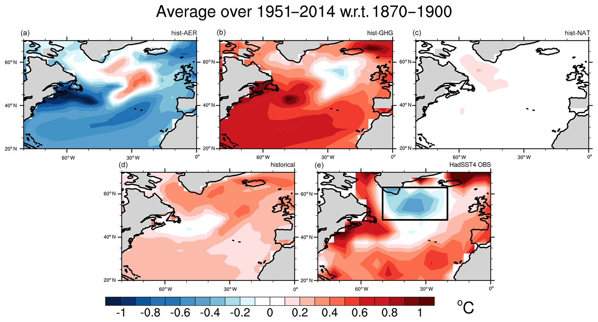
Figure 1 (a) Annual SST multimodel mean difference between the 1951–2014 and 1870–1900 periods for the CMIP6 hist-AER simulations. (b) Same as (a) but for hist-GHG. (c) Same as (a) but hist-NAT. (d) Same as (a) but for historical. (e) HadSST4 SST annual anomalies over the 1951–2014 period relative to the 1870–1900 period.

The combination of CMIP6 models and observations via the KCC statistical method provides estimates of the SST forced responses to different external forcings with uncertainties that are consistent with the available observations and internal variability. Here, I apply the KCC method to the DAMIP ensemble by using the observed SST annual time series over the warming hole, defined as the spatial average over 48, 63^∘ N and −50, −20^∘ W (see black domain in Fig. 1e), over the 1870–2021 period. As a first step, this domain is common to all models.

Figure 2 shows the attribution results over the 1951–2020 period compared to the 1870–1900 period. The contribution of all external (ALL) forcings is a cooling of the warming hole, with a best estimate of $-\mathrm{0.14}\pm \mathrm{0.12}$ ^∘C, which is half of the observed cooling ($-\mathrm{0.3}\pm \mathrm{0.12}$ ^∘C). The constrained ALL response is opposite in sign to the unconstrained response from the CMIP6 ensemble, which indicates an underestimation of the cooling, consistent with Fig. 1d. The uncertainty in the ALL response is reduced by about 70 % compared to the unconstrained response. The contributions from natural (NAT) and anthropogenic (ANT) forcings (contributing to ALL) are examined. The response due to natural NAT forcings has a very small contribution, with a slight warming of $+\mathrm{0.06}\pm \mathrm{0.02}$ ^∘C. Note that this estimate is consistent with the hist-nat simulations. The major contribution of the ALL-induced cooling comes from the ANT component, with a cooling of $-\mathrm{0.24}\pm \mathrm{0.12}$ ^∘C and a reduction of 70 % in the uncertainty, which now excludes positive values. This decrease in uncertainty is almost equally distributed between the GHG response and the response to other anthropogenic (OA, which includes aerosols, ozone…) forcings, with a decrease in uncertainty of about 65 % in both components. Note that the unconstrained OA response (estimated as the ANT minus GHG difference) is consistent with the hist-aer ensemble (Fig. S4). As the uncertainty in the constrained GHG and OA terms is still sampling both positive and negative values, it is not possible to provide a clear contribution of these forcings over the historical period.

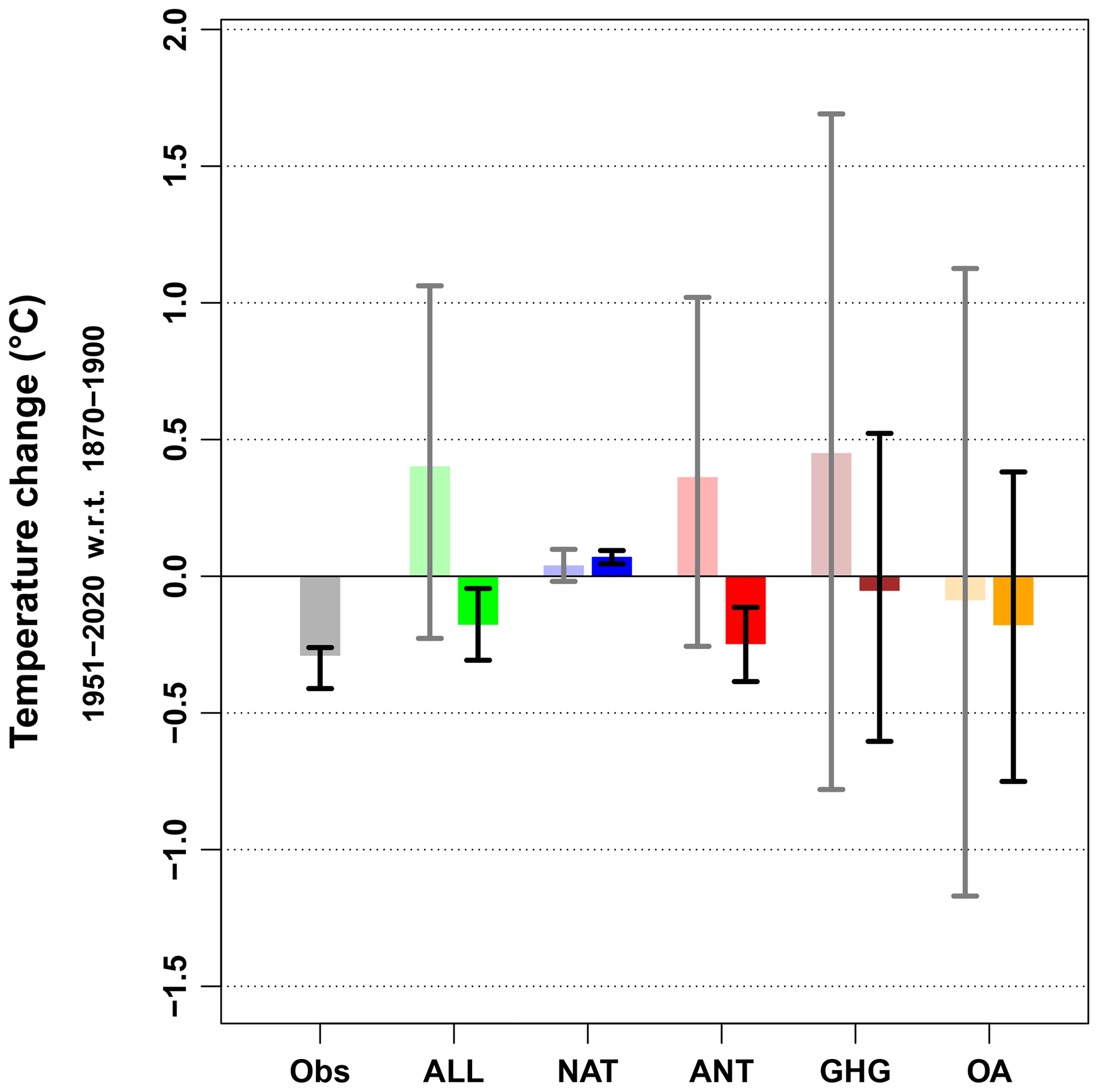
Figure 2 Changes induced by various subsets of external forcings over the historical period (1951–2020 with respect to (w.r.t.) 1870–1900) over the warming hole. Observed (Obs) changes (gray, left) are deduced from HadSST4 observations; uncertainty only includes observational uncertainty (i.e., measurement and processing; internal variability is ignored). For all other contributions, the bar and gray confidence interval on the left-hand side describe the DAMIP model range, assuming a Gaussian distribution. The bar and black confidence interval on the right-hand side correspond to results constrained by observations. All ranges shown are 5 % to 95 % confidence ranges. The SSP2-4.5 scenario is used to extend historical simulations after 2014.

The sensitivity of these attribution results to methodological factors is quantified by considering several aspects. First, to take into account the diversity of the CMIP6 models in the spatial structure of the simulated WH, the SST spatial average is defined for each model over a specific domain, to ensure a consistent comparison with observations. As done by Menary and Wood (2018), in each model, the WH is based on a domain where a noticeable warming over the subpolar gyre in the hist-AER simulations is colocated with a non-warming (or cooling) area in the hist-GHG simulation over the 1951–2021 period (see black boxes in Figs. S5–S6). Note that this ad hoc selection is relevant since for all models, the anomalies are co-located with the climatology estimated from the piControl simulations for most models (Fig. S7). Figure S8 shows that the consideration of this adaptive definition of the WH changes the best-estimate values of the GHG and OA response compared to Fig. 2 with refined estimations. The impact of the aerosols is an increase in SST which is opposed to the effect of GHGs. The latter largely contribute to the cooling of the WH, with an uncertainty reduced by almost half.

The second sensitivity test is to consider the full set of CMIP6 models available to estimate the forced responses, such that a sample of 27 models is considered instead of the only 12 models that contributed to the DAMIP ensemble, which may undersample internal variability and model uncertainty. Using the KCC method, hist-GHG-like simulations for the models that did not contribute to the DAMIP ensemble are reconstructed through the 1 %–CO₂ simulations (in which the CO₂ concentration increases by 1 % each year for 150 years), as done by Ribes et al. (2021) (see their Supplement Sect. 1.4). The inclusion of all CMIP6 models slightly affect the uncertainty ranges but does not change the main conclusions about the attribution of the observed cooling of the WH (Fig. S9).

3.2 Constraining projections

The KCC method is also used to constrain the SST projections associated with the CMIP6 SSPs simulations over the WH. Since DAMIP simulations are not required to perform the calculations based only on the ALL component, all available CMIP6 models are used to estimate the past and future forced responses, using a fixed WH domain as in Fig. 2. Figure 3 shows that the uncertainty in the three selected scenarios is reduced by 65 % for a mid-time period (2041–2060), and by 50 % at the end of the 21st century compared to the unconstrained projections. The lower bound of the projected distributions is less affected than the upper bound. For example, in 2100 for the SSP2-4.5 simulation, the constrained lower bound of −0.76 ^∘C is revised upwards compared to the unconstrained bound (−2.08 ^∘C), while the upper bound is revised downwards considerably (+2.34 and +4.59 ^∘C for the constrained and unconstrained values, respectively). Consequently, trajectories associated with a very strong warming of the WH are excluded from the posterior distribution (i.e., after the constraint). Note that this posterior distribution over the projected period largely surrounds the 0 ^∘C value. This indicates that even if a considerable warming of the WH is less likely in the future, projections remain uncertain about the sign relative to the future SST changes.

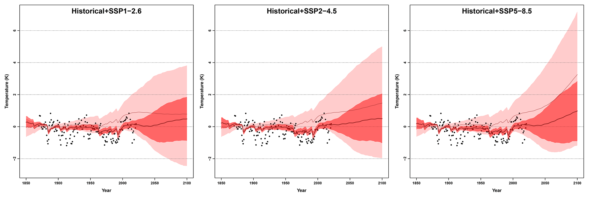
Figure 3 The observational constraint is applied to concatenated historical and SSP scenarios simulations (SSP1-2.6, SSP2-4.5, or SSP5-8.5). Annually observed values of SST over the warming hole (black points) are compared to the unconstrained (pink) and constrained (red) 5 % to 95 % confidence ranges of forced response as estimated from 27 CMIP6 models. All temperatures are anomalies with respect to the period 1870–1900.

In order to evaluate the confidence in these results, the KCC method is applied within a perfect model framework, following a leave-one-out cross-validation.

• For a given model, a single member is considered as pseudo-observations y over the 1850–2021 period (the historical simulation is extended by the SSP2-4.5 simulation over the 2015–2021 period).

• The other 26 models are used to derive the prior distribution $\mathrm{\Pi }\left(\mathit{x}\right)\sim \mathcal{N}({\mathit{\mu }}_x,{\mathbf{\Sigma }}_x)$.

• As done with the real observations, internal variability within the pseudo-observations is estimated from the difference between the time series of pseudo-observations and the forced temperature response estimated by the ensemble mean of the 26 other models. Then, Σ_y is derived from the MAR model fitted on the obtained residuals, following the same iterative way detailed in Eq. (D3).

• The KCC method is applied using the inputs y, Σ_y, μ_x and Σ_x to calculate projected changes constrained by the pseudo-observations, extracted from the SSP2-4.5 simulation.

• These four steps are repeated for each available member of the considered model and for all available models.

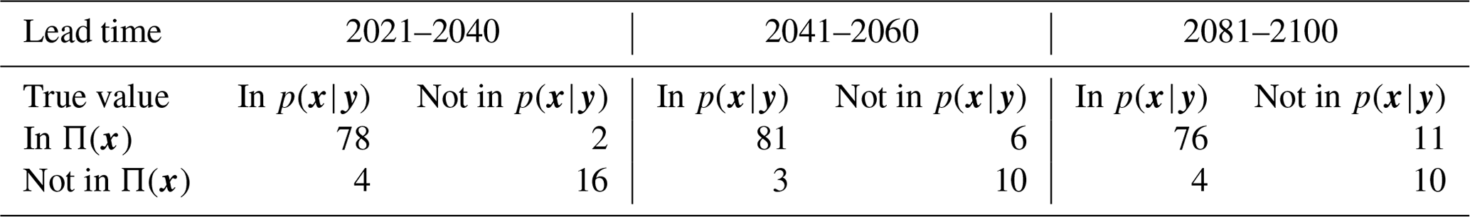
I use the confusion matrix to estimate the reliability of the method for the short- (2021–2040), mid- (2041–2060) and long-term (2081–2100) periods (Table 1). This matrix aims to quantify the coverage probabilities, derived from the number of cases for which the true value (from the pseudo-obs)

• is included in both the constrained range p(x|y) and the unconstrained range Π(x) (true positive rate),

• not included in both the constrained and unconstrained ranges (true negative rate),

• is included in the constrained range but not in the unconstrained range (false positive rate),

• is included in the unconstrained range but not in the constrained range (false negative rate).

The constrained distributions contain the true values from the pseudo-observations in 80 % up to 84 % of the cases, which is close to the expected value of 90 %. The significance of this result is assessed with a binomial test. Under the null hypothesis that the probability of success is equal to 90 %, the obtained coverage probabilities remain compatible with 90 % (p value = 0.18 for a coverage probability of 80 %). Note that for this test, the number of degrees of freedom is the number of models rather than the total number of members (where there is a dependency between the members of a given model) to ensure the assumption of independence of the trials. The rate of false prediction (i.e., when the constrained distribution does not contain the true value while the unconstrained distribution does) remains very low, especially over the 2021–2040 period. Note that in about 10 % of the cases, the true value is not contained in both the constrained and unconstrained distributions. This could be explained by a high or low sensitivity of some models to external forcings in the projections compared to what is predicted by the other (unconstrained) models.

Table 1 Confusion matrix relating the temperature projection constrained by the KCC method and the true value from pseudo-observations. Rates (in %) are computed from 249 members (from 27 models) for the SSP2-4.5 simulation. Each rate is normalized by the number of ensemble members for each model to avoid giving too much weight to models with a large ensemble.

As a second performance criterion to assess the error on the amplitude of the constrained SST projections, I use the continuous ranked probability skill score (CRPSS), defined as the relative error between the constrained distribution p(x|y) and a given reference (Hersbach, 2000). Here, I quantify the added value of the constraint by considering the unconstrained projections as a benchmark. Figure 4 shows positive CRPSS values, associated with a reduction in error of 35 %, 30 % and 20 % on average for the constrained projections compared to the raw CMIP6 projections for the short-, mid- and long-term period, respectively. The added value of the method is stronger for the short-term than for the long-term period, as observations are temporally closer for the former. Overall, these results demonstrate that the results from the method are not overconfident and that the constrained uncertainty ranges are reliable.

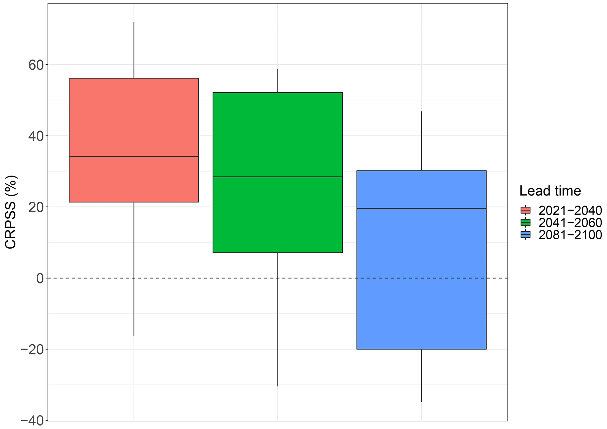
Figure 4 CRPSS for the constrained SST projections over the WH within the perfect model framework. The red, green and blue boxplots indicate the CRPSS distributions for different lead times. Calculation is made for all CMIP6 ensemble members (see Table A1). The top (bottom) of the box represents the 25th (75th) percentile of the distribution and the upper (lower) whisker represents the 95th (5th) percentile. Values are normalized by the number of members in each model. A CRPSS of 0 (dashed line) indicates the absence of added values of the method.

4 Conclusions

The temperature response to external forcings on the North Atlantic warming hole (WH) over the past and future period is estimated by the KCC statistical method based on kriging techniques, which combines climate models and observations. Consistent with the observations, an anthropogenic cooling is diagnosed by the method over the last decades (1951–2021) compared to the preindustrial period. The impact of the aerosols is an increase in SST which is opposed to the effect of GHGs. The latter largely contribute to the cooling of the WH over the historical period. Although the anthropogenic response is clear, the respective contribution of each anthropogenic forcing is associated with large uncertainties, especially for the aerosols. The quantification is in line with previous studies (Dagan et al., 2020; Chemke et al., 2020) that suggest that GHGs and aerosols have had compensating effects on the evolution of the WH. In the present study, the attribution of the temperature changes is based on only 12 models. Although the CMIP6 ensemble shows qualitatively consistent results, this large uncertainty points to the crucial need to increase the number of models running single forcing experiments as done in DAMIP to better sample the model uncertainty. The method is also applied to CMIP6 projections and is able to reduce the model uncertainty in the anthropogenic response by a factor of 3 over the historical period and by a factor of 2 in the long-term projections. In particular, models projecting strong SST increase over the WH are excluded from the likely range constrained by the method.

This result has important implications for the estimation of the future changes in terms of teleconnection processes between the North Atlantic and the continental climate, e.g., over Europe, North America or the Sahelian monsoon. It would be interesting to re-evaluate the climate impacts of the North Atlantic SST variability in light of the constrained temperature ranges obtained in this study, e.g., in terms of the occurrence of extreme events or changes in atmospheric circulation.

A relevant perspective of these results is the potential constraint of the Atlantic Meridional Overturning Circulation (AMOC). Using the same approach as in this paper and to directly constrain future AMOC changes is challenging due to the limited number of observations monitored via the RAPID program (Frajka-Williams et al., 2021). Instead, it is possible to take advantage of the covariance between the AMOC and proxies based on SST and salinity over the North Atlantic (Zhang, 2017; Caesar et al., 2018) and to apply the kriging method to these proxies. This approach will allow a better estimation of the uncertainty in the forced response included in these proxies, which could lead to revised estimates of the AMOC forced response over the past and future periods.

Appendix A: List of the CMIP6 models

Table A1 List of the available CMIP6 Models and the associated number of members in the simulations used to constrain the temperature time series.

Appendix B: Structure of the observation operator H

The observation operator H is a matrix of size n_y×n_x. The constraint by both GSAT and regional observations comprises setting the submatrices ${\mathbf{H}}_{\mathrm{reg}}={\mathit{I}}_{\mathrm{1870}:\mathrm{2021}}$ and ${\mathbf{H}}_{\mathrm{glo}}={\mathit{I}}_{\mathrm{1850}:\mathrm{2021}}$ and all other coefficients equal to zero (see block matrices in Eq. B1). This structure allows the extraction of the appropriate years from the vector x (see Eq. 2). As an example, the vector of the GSAT forced response from 1850 to 2100 is of size $n_{x,\mathrm{glo}}=\mathrm{251}$, while the vector of the GSAT observations from 1850 to 2021 is of size $n_{y,\mathrm{glo}}=\mathrm{172}$. Hence, the operator H_glo is of size $n_{y,\mathrm{glo}}\times n_{x,\mathrm{glo}}$, which extracts the part of the GSAT forced response that matches the GSAT observations, i.e., the GSAT forced response from 1850 to 2021. The same is done for the SST over the warming hole through the operator H_reg.

$$\begin{array}{}\text{(B1)}& {\displaystyle }\mathbf{H}=\left[\begin{array}{cccccc}{\mathbf{H}}_{\mathrm{glo}}& \mathbf{0}& \mathbf{0}& \mathbf{0}& \mathbf{0}& \mathbf{0}\\ \mathbf{0}& {\mathbf{H}}_{\mathrm{reg}}& \mathbf{0}& \mathbf{0}& \mathbf{0}& \mathbf{0}\end{array}\right]\end{array}$$

Appendix C: Modeling of Σ_x

The DAMIP (or CMIP6) multimodel ensemble is used to derive a distribution of x, denoted as $\mathrm{\Pi }\left(\mathit{x}\right)\sim \mathcal{N}({\mathit{\mu }}_x,{\mathbf{\Sigma }}_x)$; μ_x is the concatenated forced responses to all and specific external forcings mentioned in Eq. (2). From each model, I derive the forced responses following Ribes et al. (2021), i.e., 12 (27) vectors, from the DAMIP (CMIP6) ensemble; Σ_x is a variance–covariance matrix of size n_x×n_x that describes the model spread. Using a sample covariance estimate has the side effect of producing a highly degenerated estimate for Σ_x: while Σ_x is an n_x×n_x matrix, the rank of Σ_x is equal to 26 (since 27 CMIP6 models are being considered). While this choice could be debated, the KCC method can be run in this way, as Σ_x does not need to be inverted to derive the parameters μ_p and Σ_p of the posterior distribution.

In the Bayesian framework, Π(x) is a first (probabilistic) estimate of x, which makes no use of observations, and is only based on climate models. I update this estimate by incorporating the observational evidence provided by y. Following the Bayesian theory, the calculation of the posterior distribution p(x|y) is required. A prerequisite is to define the observational uncertainty, i.e., the covariance matrix associated with y.

Appendix D: Modeling of Σ_y

The matrix Σ_y is estimated by using observed annual time series of GSAT and SST temperature over the historical period. First, I compute the global observational residuals by subtracting the CMIP6 GSAT response (multimodel mean) to all external forcings from the observations ${\mathit{T}}_{\mathrm{glo}}^{\mathrm{obs}}$. Similarly, I derive regional residuals over the WH by subtracting the CMIP6 SST response from ${\mathit{T}}_{\mathrm{reg}}^{\mathrm{obs}}$. These residuals constitute a first estimate of global and regional internal variability, denoted as ${\widehat{\mathit{ϵ}}}_{y,\text{glo},\mathrm{1}}$ and ${\widehat{\mathit{ϵ}}}_{y,\text{reg},\mathrm{1}}$, respectively.

I define Σ_y as a matrix of size n_y×n_y of the following form:

$$\begin{array}{}\text{(D1)}& {\displaystyle }{\mathbf{\Sigma }}_y=\left[\begin{array}{cc}{\mathbf{\Sigma }}_{y,\text{reg}}& {\mathbf{\Sigma }}_{y,\text{dep}}\\ {\mathbf{\Sigma }}_{y,\text{dep}}^{\prime }& {\mathbf{\Sigma }}_{y,\text{glo}}\end{array}\right],\end{array}$$

where Σ_y,reg and Σ_y,glo are the covariance matrices modeling regional and global internal variability within ${\mathit{T}}_{\mathrm{reg}}^{\mathrm{obs}}$ and ${\mathit{T}}_{\mathrm{glo}}^{\mathrm{obs}}$, respectively; Σ_y,dep is the covariance matrix modeling the dependence between regional and global internal variability, i.e., ϵ_y,reg and ϵ_y,glo.

To compute Σ_y, I take into account decadal internal variability that may exist in the global (Parsons et al., 2020) and regional (Qasmi et al., 2017) observations by using a mixture of two autoregressive processes of order 1 (AR1), hereafter MAR, as done by Qasmi and Ribes (2022). The MAR formulation includes fast (f) and a slow (s) components such that global internal variability ϵ_y,glo within the GSAT residuals writes at a time t:

$$\begin{array}{}\text{(D2)}& {\displaystyle }\left\{\begin{array}{ll}{\mathit{ϵ}}_{y,\text{glo}}\left(t\right)& ={\mathit{ϵ}}_{y,\text{f,glo}}\left(t\right)+{\mathit{ϵ}}_{y,\text{s,glo}}\left(t\right),\\ {\mathit{ϵ}}_{y,\text{f,glo}}\left(t\right)& ={\mathit{\alpha }}_{\mathrm{f},\mathrm{glo}}{\mathit{ϵ}}_{y,\text{f,glo}}(t-\mathrm{1})+Z_{\mathrm{f},\mathrm{glo}}\left(t\right),\\ {\mathit{ϵ}}_{y,\text{s,glo}}\left(t\right)& ={\mathit{\alpha }}_{\mathrm{s},\mathrm{glo}}{\mathit{ϵ}}_{y,\text{s,glo}}(t-\mathrm{1})+Z_{\mathrm{s},\mathrm{glo}}\left(t\right),\end{array}\right.\end{array}$$

where the parameters α_s,glo and α_f,glo are the lag 1 coefficients of the AR1 processes and ${\mathit{\alpha }}_{\mathrm{s},\mathrm{glo}}\ge {\mathit{\alpha }}_{\mathrm{f},\mathrm{glo}}$ by convention; $Z_{\mathrm{s},\mathrm{glo}}\left(t\right)\sim \mathcal{N}(\mathrm{0},{\mathit{\sigma }}_{\mathrm{s},\mathrm{glo}}^{\mathrm{2}}$) and $Z_{\mathrm{f},\mathrm{glo}}\left(t\right)\sim \mathcal{N}(\mathrm{0},{\mathit{\sigma }}_{\mathrm{f},\mathrm{glo}}^{\mathrm{2}}$) are white noises associated with the two AR1. The slow component is able to generate a dependence on timescales of typically one decade, while the fast component accounts for interannual variability. The covariance matrix Σ_y,glo is filled according Sect. D2. The same assumptions are adopted to estimate the regional parameters and to compute Σ_y,reg.

The initial estimate of Σ_y, denoted as ${\widehat{\mathbf{\Sigma }}}_{y,\mathrm{1}}$ is solely based on the residuals ${\widehat{\mathit{ϵ}}}_{y,\text{reg},\mathrm{1}}$ and ${\widehat{\mathit{ϵ}}}_{y,\text{glo},\mathrm{1}}$ derived from the unconstrained forced response. This first estimate is likely flawed as the real (and unknown) forced response is not necessarily consistent with the unconstrained forced response estimated by μ_x. In addition, as μ_x can by construction be different from the best estimate of the constrained forced response ${\widehat{\mathit{\mu }}}_{\mathit{x}\mathbf{,}\mathbf{1}}$ (the mean of the posterior distribution p(x|y)), the residuals ${\widehat{\mathit{ϵ}}}_{y,\text{reg},\mathrm{1}}$ and ${\widehat{\mathit{ϵ}}}_{y,\text{glo},\mathrm{1}}$ before constraint are not always coherent with the residuals ${\widehat{\mathit{ϵ}}}_{y,\text{reg},\mathrm{2}}$ and ${\widehat{\mathit{ϵ}}}_{y,\text{glo},\mathrm{2}}$ computed as the $\mathit{y}-{\widehat{\mathit{\mu }}}_{\mathit{x}\mathbf{,}\mathbf{1}}$ difference.

Hence, in order to ensure an accurate estimation of internal variability in the constraint procedure, an iterative algorithm is applied to find the MAR parameters that fit the residuals from the constrained forced response:

$$\begin{array}{l}\text{(D3)}& {\displaystyle }\mathit{y}-\mathit{\mu }\stackrel{\text{residuals}}{⟶}{\widehat{\mathit{ϵ}}}_{y,\mathrm{1}}\stackrel{\text{constraint}}{⟶}\widehat{{\mathit{\mu }}_{\mathbf{1}}},{\displaystyle }\mathit{y}-\widehat{{\mathit{\mu }}_{\mathbf{1}}}\stackrel{\text{residuals}}{⟶}{\widehat{\mathit{ϵ}}}_{y,\mathrm{2}}\stackrel{\text{constraint}}{⟶}\widehat{{\mathit{\mu }}_{\mathbf{2}}},\\ {\displaystyle }\mathrm{\dots }\\ {\displaystyle }\mathit{y}-{\widehat{\mathit{\mu }}}_{\mathit{n}\mathbf{-}\mathbf{1}}\stackrel{\text{residuals}}{⟶}{\widehat{\mathit{ϵ}}}_{y,n}\stackrel{\text{constraint}}{⟶}\widehat{{\mathit{\mu }}_{\mathit{n}}},\end{array}$$

where for each iteration n, $\widehat{{\mathit{\mu }}_{\mathit{n}}}$ and ${\widehat{\mathit{ϵ}}}_{y,n}$ are estimates of the forced response and internal variability, respectively. The termination criterion is based on the Frobenius norm $\left|\right|.|{|}_F$. Hence, I consider that the algorithm converges at the iteration n, i.e., that ${\widehat{\mathit{ϵ}}}_{y,n}\to {\mathit{ϵ}}_y$, when the relative difference between $\left|\right|{\widehat{\mathbf{\Sigma }}}_{y,n}|{|}_F$ and $\left|\right|{\widehat{\mathbf{\Sigma }}}_{y,n-\mathrm{1}}|{|}_F$ is inferior to 1 %, implying that the MAR parameters values have converged. In practice, only two iterations are necessary in this study.

Initial-condition large ensembles and long piControl simulations provide a nice sampling of internal variability and could also be used to estimate this variability. However, I choose to not rely on it directly because of the huge discrepancies between models in terms of their simulated internal variability (Parsons et al., 2020). Qasmi and Ribes (2022) have illustrated this aspect with the piControl simulations from the CMIP6 models, including those used to build large ensembles. In all cases, the models do not converge to a consistent estimate of internal variability over the WH.