Emergent constraints for the climate system as effective parameters of bulk differential equations

Planning for the impacts of climate change requires accurate projections by Earth system models (ESMs). ESMs, as developed by many research centres, estimate changes to weather and climate as atmospheric greenhouse gases (GHGs) rise, and they inform the influential Intergovernmental Panel on Climate Change (IPCC) reports. ESMs are advancing the understanding of key climate system attributes. However, there remain substantial inter-ESM differences in their estimates of future meteorological change, even for a common GHG trajectory, and such differences make adaptation planning difficult. Until recently, the primary approach to reducing projection uncertainty has been to place an emphasis on simulations that best describe the contemporary climate. Yet a model that performs well for present-day atmospheric GHG levels may not necessarily be accurate for higher GHG levels and vice versa.

A relatively new approach of emergent constraints (ECs) is gaining much attention as a technique to remove uncertainty between climate models. This method involves searching for an inter-ESM link between a quantity that we can also measure now and a second quantity of major importance for describing future climate. Combining the contemporary measurement with this relationship refines the future projection. Identified ECs exist for thermal, hydrological and geochemical cycles of the climate system. As ECs grow in influence on climate policy, the method is under intense scrutiny, creating a requirement to understand them better. We hypothesise that as many Earth system components vary in both space and time, their behaviours often satisfy large-scale differential equations (DEs). Such DEs are valid at coarser scales than the equations coded in ESMs which capture finer high-resolution grid-box-scale effects. We suggest that many ECs link to such effective hidden DEs implicit in ESMs and that aggregate small-scale features. An EC may exist because its two quantities depend similarly on an ESM-specific internal bulk parameter in such a DE, with measurements constraining and revealing its (implicit) value. Alternatively, well-established process understanding coded at the ESM grid box scale, when aggregated, may generate a bulk parameter with a common “emergent” value across all ESMs. This single emerging parameter may link uncertainties in a contemporary climate driver to those of a climate-related property of interest. In these circumstances, the EC combined with a measurement of the driver that is uncertain constrains the estimate of the climate-related quantity. We offer simple illustrative examples of these concepts with generic DEs but with their solutions placed in a conceptual EC framework.

1 Introduction

Earth system models (ESMs) are a key pillar of climate research and provide predictions of global environmental change due to burning fossil fuels. Projections by ESMs strongly inform the reports of the Intergovernmental Panel on Climate Change (e.g. IPCC, 2013, 2021) and influence climate policy. These models consist of solving, on numerical meshes, discretised differential equations that describe the evolution of the atmosphere, oceans, land and cryosphere and their interactions. In addition to physical processes, these models have evolved to emulate key global geochemical cycles. ESMs are typically forced with prescribed values of historical atmospheric greenhouse gas (GHG) concentrations, followed by a range of scenarios for their future levels (e.g. Meinshausen et al., 2011). This process estimates how the planetary climate system responds to altered atmospheric gas composition. Alternatively, an ESM can be forced with CO₂ emissions scenarios (e.g. Cox et al., 2000), if the ESM has a complete description of the global carbon cycle. A major achievement of the scientific community is the pooling of climate model projections from different research centres into common Coupled Model Intercomparison Project (CMIP) databases such as CMIP5 (Taylor et al., 2012) and CMIP6 (Eyring et al., 2016). CMIP databases also hold simulations with forcings held at pre-industrial levels to test ESM stability and characterise their representation of natural variability. Furthermore, there exist illustrative idealised ESM experiments, to determine the response to a continuous cumulative 1 % per annum increase in atmospheric CO₂, or to an abrupt jump by a factor of 4 in CO₂ from pre-industrial levels.

Almost all parts of the climate system vary in both space and time. Hence partial differential equations (PDEs) are solved for evolving temporal variations on the spatial numerical mesh particular to any ESM. Many of these PDEs central to understanding the climate system are well-established, as described in standard textbooks on atmospheric and oceanic behaviours (e.g. Vallis, 2017). However, for the same future GHG scenario, analyses of the CMIP databases reveal significant inter-ESM differences between projections of even fundamental quantities such as the level of global warming (Lee et al., 2021). As standard equations are frequently solved in ESMs, a valid question is why are ESM projections often so different? The simplest answer is that some processes are still not fully understood and are therefore parameterised differently between ESMs. Components frequently noted in this category are the modelling of cloud–climate interactions (e.g. Bony et al., 2015) and how aerosols act in modulating global temperature rise (e.g. Bellouin et al., 2020). A secondary source of uncertainty is the dependence of process parameterisation on grid box resolution. Larger individual grid boxes (i.e. a coarser numerical grid) often need effective parameterisation of sub-grid processes, and variation in this may cause inter-ESM differences. Numerical tests with extremely high-resolution models allow the explicit representation of convection (“convection permitting”; e.g. Clark et al., 2016) and verify its importance in describing local rainfall characteristics. However, while very high resolutions are achievable in weather forecast models, computational speed precludes their routine operation for ESMs designed to simulate century timescales.

Unfortunately, the considerable variation in model estimates of future climate change makes societal adaptation planning difficult. Such discrepancies can be used by some to discredit the overall notion of a human influence on climate. One possibility to lower inter-ESM spread is to rank models by their ability to describe the contemporary climate and known recent changes (e.g. Knutti et al., 2017). ESMs regarded as the most reliable at describing expected future change are those that perform best at simulating the recent past. However, this can be a subjective activity, depending on selected datasets for comparison and geographical location analysed. Furthermore, there is a risk of downrating a model that performs poorly for the present day yet accurately projects a future change of concern to society.

Recently a technique called “emergent constraints” (ECs) has gained prominence as a new method to reduce the spread between the projections by different ESMs. The EC method capitalises on discovered relationships between two quantities calculated by climate models when considering estimates of each from across many ESMs. One variable is an attribute of the climate system for the present day or historical period, for which observationally based data also exist. The second variable, for which data are unavailable, is often a feature of the evolving climate system and is informative for climate policy. For example, this second variable may be an internal sensitivity of the climate system that determines changes to mean meteorological conditions as GHGs rise. Alternatively, it can be the direct estimate of some feature of climate change (e.g. an aspect of near-surface meteorology) corresponding to specific future higher GHG levels. Measurement of the first quantity, in combination with the discovered inter-ESM link between the two variables (i.e. the EC), provides the constraint on the magnitude of the second unknown variable.

The first applications of the EC technique were to constrain estimates of transient climate response (TCR) and mean precipitation changes for different warming levels (Allen and Ingram, 2002) and to refine estimates of large-scale snow albedo feedbacks in a warming world (Hall and Qu, 2006). Since then, the EC method has lowered uncertainty in a substantial number of components of the Earth system (Hall et al., 2019) and including for fundamental climate quantities such as equilibrium climate sensitivity (ECS) (e.g. Cox et al., 2018). Other researchers have provided EC-based estimates of both ECS and TCR (Jimenez-de-la Cuesta and Mauritsen, 2019; Nijsse et al., 2020; Tokarska et al., 2020). Applications of ECs to physical parts of the Earth system have included cloud feedbacks (e.g. Klein and Hall, 2015), as well as components of global geochemical cycles. ECs on aspects of geochemical cycles include constraining the expected level of ocean acidification (Terhaar et al., 2020), marine primary productivity (Kwiatkowski et al., 2017) and soil carbon turnover (Varney et al., 2020). Notable is that for many discovered ECs, the modelled quantity that is also measured during the contemporary period is often a high-frequency statistic or attribute of the climate system. The EC relates this quantity that fluctuates at shorter timescales to a longer-term attribute of the Earth system relevant to projecting how climate will respond to rising GHG concentrations. The ability of ECs to use knowledge of contemporary high-frequency variations to constrain understanding of expected future climate change highlights how ignoring fluctuations at short timescales may constitute disregarding valuable information. The EC approach, therefore, offers an interesting comparison to the method of weighting ESMs by simply comparing their projections of present-day trends against measurements, especially as the latter method often neglects short-timescale variations about such trends.

With ECs becoming ubiquitous in climate research and with their potential to enable better decisions on GHG emissions trajectories that avoid dangerous change, it is appropriate that the method is placed on a stronger scientific basis. Some recent papers review the EC method, highlighting its capability and listing a set of potential pitfalls. For instance, Williamson et al. (2021) identify a particularly broad range of discussion points related to ECs, all framed in their application to refining estimates of ECS. Further critiques of the EC method exist in the context of the terrestrial carbon cycle (Winkler et al., 2019), Arctic warming (Bracegirdle and Stephenson, 2012) and ECS (Caldwell et al., 2018) – all note potential issues that could result in incorrect bounds on future estimates of change. Schlund et al. (2020) test the robustness of proposed emergent constraints by out-of-sample testing on a different model ensemble. These researchers found that emergent constraints on ECS, developed using the CMIP5 ensemble, do not provide useful constraints on ECS in the CMIP6 models. These ECs, therefore, fail to be “confirmed” (Hall et al., 2019). Fasullo et al. (2015) also discuss whether it is expected that ECs hold across different generations of ESMs. Those authors argue that additional processes identified as important but uncertain, and introduced to newer ensembles, could generate ECs that make different predictions. Fasullo et al. (2015) provide the example of newer ESMs that characterise better convection and its impact on simulated cloud features, which ultimately may alter EC estimates of ECS. Recognising the danger of arriving at spurious emergent constraints based on the results of relatively small model ensembles (Caldwell et al., 2018), Williamson et al. (2021) have set the challenge of deriving more robust theory-based emergent constraints. To inform attempts to meet that challenge, here we address the fundamental, almost philosophical question: What is an emergent constraint?

Despite much scrutiny of ECs, there are likely many perspectives on what forms their basis (see for example Nijsse and Dijkstra, 2018; Williamson et al., 2021). Here we suggest that one way to interpret many ECs is that they derive bulk parameters associated with differential equations that are valid at large spatial scales. Such equations are implicit in ESMs (i.e. are not coded explicitly) and instead “emerge” by aggregating the numerical finite difference schemes solved in ESMs at the finer grid-box spatial resolution. Here we hope to initiate a discussion of whether this is an appropriate way to describe the underpinning properties of many ECs. We consider simple illustrative examples using standard solutions to basic differential equations but with the novelty of being placed in the context of the framework of the EC method.

2 Methods and conceptual examples

2.1 The emergent constraint method

The core of any EC is the discovery of a robust link, across different ESMs, between a driving variable, say X, and another model-calculated quantity, Y. Variable X is a quantity for which contemporary measurements are available. Quantity Y is a climate-related statistic, metric or parameter often of importance for developing future adaptation or mitigation strategy, but for which data do not exist. The EC relationship between X and Y, in tandem with the measurement of X, constrains our understanding of Y. In general, it is considered preferable that ECs are found by process intuition that reveals related system quantities, rather than direct inter-ESM “data mining”. For instance, in the context of finding ECs to constrain understanding of the size of cloud feedbacks, Klein and Hall (2015) propose that each should be “accompanied by credible physical explanations”. The EC relationship between X and Y may take many forms, such as a nonlinear response, or is potentially multidimensional with more than one X component.

For illustration purposes, we imagine an EC that is a simple linear regression between two variables and when indexing each ESM with i is of the form

$$\begin{array}{}\text{(1)}& Y_i=a_{\mathrm{0}}+a_{\mathrm{1}}{X}_i+{\mathit{ϵ}}_i+{\mathit{\eta }}_i.\end{array}$$

Here parameters a₀ and a₁ quantify the emergent constraint, and ϵ_i and η_i are ESM-specific “noise” terms. We consider that ϵ_i captures how far an individual ESM is from the fitted relationship of Eq. (1), and so any large absolute value corresponds to a model outlier. Quantity η_i is a random variable that describes natural climate variability for each model. Measurement X^* utilises this relationship to predict the value of Y, named Y^*. Cox et al. (2018) provide the methodology to derive uncertainty bounds on the constrained value Y^*, which include being a function of ϵ and η, as well as the size of uncertainty bounds on data X^*. Here, and elsewhere, the “∗” symbol represents a measurement (or a value constrained by an EC and a measurement).

2.2 Simple thermal “box” model with different heat capacities

Our working assumption is that ECs exist due to common inter-ESM deterministic processes, which we attempt to mirror with abstract but illustrative simple models. As such, the noise quantities ϵ_i and η_i are only reconsidered towards the end of our analysis and then only visually. We start with an especially simple conceptual representation of an EC. We consider a set of single thermal box models indexed by i. This indexing may mirror the differentiation between ESMs in a collection of models, such as the CMIP6 ensemble (Eyring et al., 2016). Each model has a different heat capacity $c_{p_i}$ (J K⁻¹), into which we assume there is a common and known forcing heat flux H(t) (W). We regard long-term changes in this forcing as analogous to representative concentration pathways (RCPs) of future GHG levels, often applied as an equal forcing across ESMs. As a single box, there is no spatial variation, so the model is treated as having infinite diffusion. The equation for the box temperature T(t) (K), where t (year) is time, $c_{p_i}^{\prime }=c_{p_i}/n_{\mathrm{y},\mathrm{s}}$ (J K⁻¹ yr s⁻¹) and n_y,s (s yr⁻¹) is the number of seconds in a year, is

$$\begin{array}{}\text{(2)}& c_{p_i}^{\prime }{\displaystyle \frac{\mathrm{d}T}{\mathrm{d}t}}=H.\end{array}$$

We first study for a known fluctuating heat flux, H=bcos (ωt), for the contemporary period to force each model indexed by i. This forcing could be interpreted as a form of known annual seasonal cycle (and therefore ω=2π), unaffected by any background trends. This driver results in a model-specific temperature, T_i(t). In addition to the known common H driver, observed are seasonal temperature features named T^∗ (K). The simple solution to Eq. (2) with this periodic forcing is

$$\begin{array}{}\text{(3)}& T_i\left(t\right)=C_{\mathrm{0}}+{\displaystyle \frac{b}{c_{p_i}^{\prime }\mathit{\omega }}}\sin \left(\mathit{\omega }t\right).\end{array}$$

Removal of background multi-year temperature allows the setting of arbitrary constant C₀ as C₀=0. ECs require a quantity that is both modelled for the contemporary period and is available as a measurement, such as the seasonal range ΔT_S (K). Here $\mathrm{\Delta }{T}_{{\mathrm{S}}_i}=max\left(T_i\right)-min\left(T_i\right)$, and so for each model and from Eq. (3),

$$\begin{array}{}\text{(4)}& \mathrm{\Delta }{T}_{{\mathrm{S}}_i}={\displaystyle \frac{\mathrm{2}b}{c_{p_i}^{\prime }\mathit{\omega }}}.\end{array}$$

Considered additionally is a longer-term forcing of our model, representing ongoing climate change. We describe this extra forcing as simply a fixed value of H₀ (W) for t>0. Hence this gives a combined forcing of $H\left(t\right)=H_{\mathrm{0}}+b\cos \left(\mathit{\omega }t\right)$, and solving Eq. (2) for both drivers simultaneously gives

$$\begin{array}{}\text{(5)}& T_i\left(t\right)={\displaystyle \frac{H_{\mathrm{0}}t}{c_{p_i}^{\prime }}}+{\displaystyle \frac{b}{c_{p_i}^{\prime }\mathit{\omega }}}\sin \left(\mathit{\omega }t\right)t>\mathrm{0}.\end{array}$$

A second set of temperature-based statistics we can consider are based on changes in annual means. The time derivative of annual averages for T is a proxy for the rate of global warming. Annual averaging of Eq. (5) and denoted by an overline is simply

$$\begin{array}{}\text{(6)}& \stackrel{\mathrm{‾}}{T_i\left(t\right)}={\displaystyle \frac{H_{\mathrm{0}}t}{c_{p_i}^{\prime }}}.\end{array}$$

A possible EC is now revealed where the issue of future concern might be the rate of change of mean temperature T_i. Plotting for the simple model an “x” axis of $\mathrm{\Delta }{T}_{{\mathrm{S}}_i}$ (from Eq. 4) and a “y” axis of $\mathrm{d}\stackrel{\mathrm{‾}}{T_i\left(t\right)}/\mathrm{d}t=H_{\mathrm{0}}/c_{p_i}^{\prime }$ (from Eq. 6) would yield a diagram where both quantities increase, linearly, in $\mathrm{1}/c_{p_i}^{\prime }$. The EC is, therefore, a relation between seasonal temperature variation and long-term warming that holds across all $c_{p_i}^{\prime }$ values. Knowledge of the actual x-axis variable, which here would be the known observed seasonal amplitude, $\mathrm{\Delta }{T}_{\mathrm{S}}^{*}$, constrains the bounds of the uncertainty of the y-axis quantity. We present these ideas schematically in Fig. 1 and show the uncertainty, ϵ_i+η_i, as just random distances by individual models (black dots) away from the EC regression line.

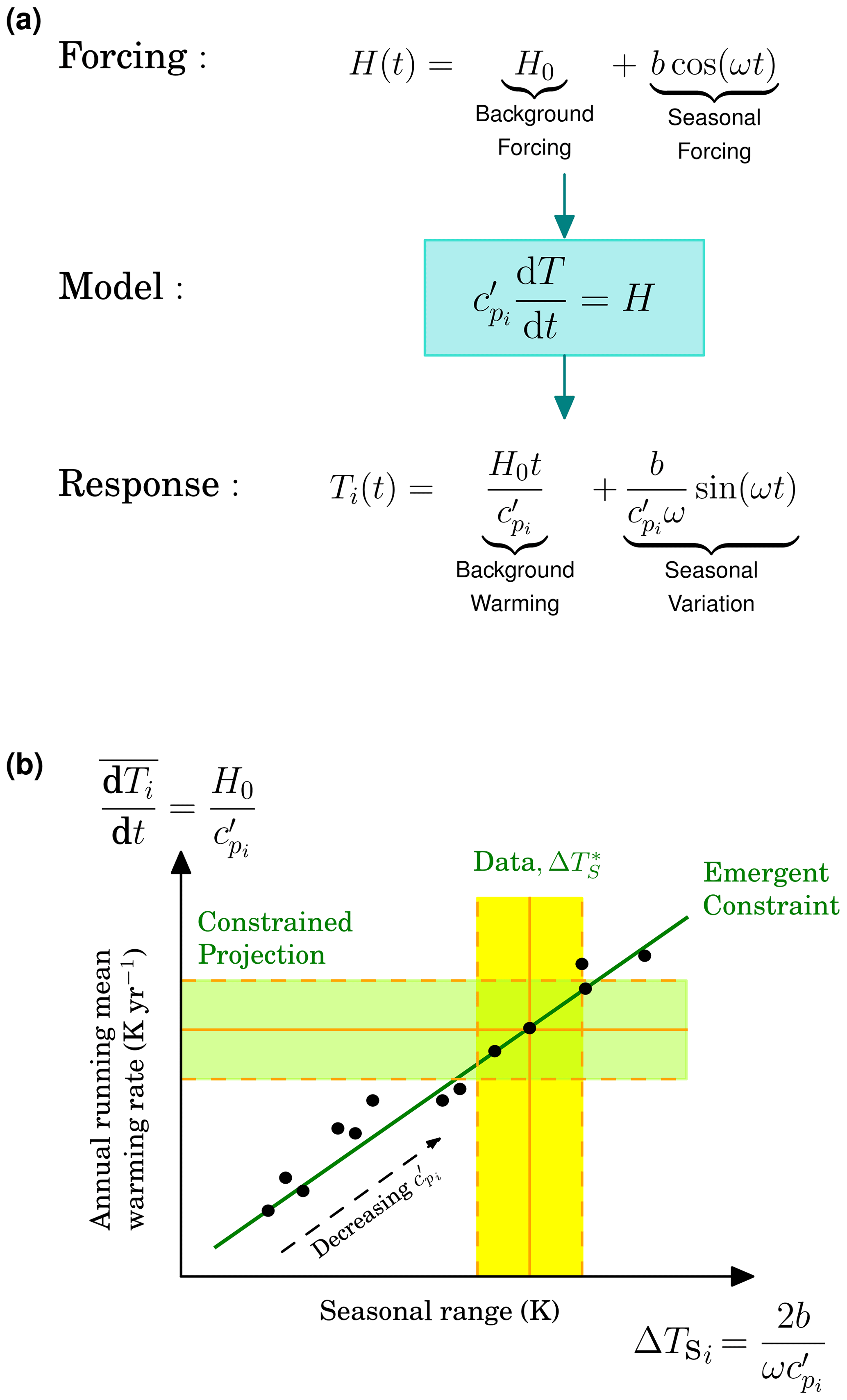
Figure 1 Schematic representation of a simple emergent constraint. Panel (a) (top row) shows the combined equation for long-term and seasonal forcing (so with ω=2π yr⁻¹) driving the thermal box model given by Eq. (2) (middle row), and the related response to both forcings, which combine additively to give Eq. (5) (bottom row). Panel (b) illustrates a related emergent constraint, based on the response Eq. (5), as also shown in (a). This response contains a seasonal (x axis) and long-term (y axis, with seasonality ignored) variation, and the EC links the two. The EC allows the observation of seasonal fluctuations ($\mathrm{\Delta }{T}_{\mathrm{S}}^{*}$, x axis) to constrain the long-term rate of change of state variable, T (y axis). Each model (black dots, indexed by i) has a different implicit value for $c_p^{\prime }$ i.e. $c_{p_i}^{\prime }$. The EC is assumed to not be exact, with noise causing variation around the regression line (the ϵ_i and η_i terms of Eq. 1). The vertical yellow band represents uncertainty in the measurement, $\mathrm{\Delta }{T}_{\mathrm{S}}^{*}$. The constrained projection of the long-term warming rate (based on the EC, the value of $\mathrm{\Delta }{T}_{\mathrm{S}}^{*}$ and its uncertainty) is given by the green horizontal band.

In the analysis presented above, the parameters related to forcings, i.e. b and H₀, are assumed to be invariant between models. The measurement in tandem with the EC is in effect lowering uncertainty on the model-specific value of bulk parameter $c_{p_i}^{\prime }$. However, an alternative possibility is an EC where there is instead uncertainty in the magnitude of the forcing of an Earth system component (rather than inter-ESM spread in how the component itself is modelled). For instance, there remains a range of representations between ESMs of translating atmospheric aerosol levels to their cooling effect. Instead, we can regard the forcing parameters as uncertain, indexed as b_i and $H_{{\mathrm{0}}_i}$, although we imagine for each ESM the uncertainty is similar, and so set the ratio $b_i/H_{{\mathrm{0}}_i}$ as invariant between models. This setup yields an EC of identical form to that of Fig. 1, but instead, $c_p^{\prime }$ has a single numerical value common to all models. Measurements then provide the constraint to remove uncertainty in the forcing element b_i. With the forcing uncertainties common for both short- and long-term drivers (i.e. the assumption that $b_i/H_{{\mathrm{0}}_i}$ is constant between ESMs), the measurement $\mathrm{\Delta }{T}_{\mathrm{S}}^{*}$ implicitly constrains b_i, hence $H_{{\mathrm{0}}_i}$, and thus the background warming $\stackrel{\mathrm{‾}}{\mathrm{d}{T}_i/\mathrm{d}t}$.

2.3 Thermal model with spatial variation

We extend the basic box model of Sect. 2.1 with a further illustrative example that introduces spatial variability via directional coordinate z (m). Temperature is retained as our notional state variable. Now we consider the system to evolve on a semi-infinite domain $\mathrm{0}\le z\le \mathrm{\infty }$, and with the heat forcing boundary condition, H, specified at z=0. This framework may depict, for instance, heat absorption by the oceans and where information on future trends in surface temperature is required. Specifically, we solve for T_i(z,t) as satisfying a diffusion equation:

$$\begin{array}{}\text{(7)}& c_{p_i}^{\prime }{\displaystyle \frac{\partial T_i}{\partial t}}={\mathit{\kappa }}_i{\displaystyle \frac{{\partial }^{\mathrm{2}}{T}_i}{\partial z^{\mathrm{2}}}}\mathrm{0}\le z\le \mathrm{\infty }.\end{array}$$

Here $c_{p_i}^{\prime }$ (J K⁻¹ m⁻³ yr s⁻¹) remains a form of heat capacity, while κ_i (W m⁻¹ K⁻¹) is a conductivity or mixing parameter, and both parameters may be model specific, as indexed by i. We again start by prescribing a boundary condition (Fourier's law of heat conduction) that is seasonal, here at z=0, given by

$$\begin{array}{}\text{(8)}& {\mathit{\kappa }}_i{\left.{\displaystyle \frac{\partial T_i}{\partial z}}\right|}_{z=\mathrm{0}}=-H=-b\cos \left(\mathit{\omega }t\right).\end{array}$$

The solution to governing Eq. (7) with the boundary condition of Eq. (8), assuming no non-seasonal transient terms and that T_i is bounded as z→∞, is

$$\begin{array}{}\text{(9)}& T_i(z,t)={\displaystyle \frac{b{e}^{-\left(z\sqrt{\frac{c_{p_i}^{\prime }\mathit{\omega }}{\mathrm{2}{\mathit{\kappa }}_i}}\right)}}{\sqrt{c_{p_i}^{\prime }{\mathit{\kappa }}_i\mathit{\omega }}}}\cos \left[-\mathit{\omega }t+{\displaystyle \frac{\mathit{\pi }}{\mathrm{4}}}+z\sqrt{{\displaystyle \frac{c_{p_i}^{\prime }\mathit{\omega }}{\mathrm{2}{\mathit{\kappa }}_i}}}\right]+C_{\mathrm{0}}.\end{array}$$

Hence the value of T_i at z=0, with additive constant set to C₀=0, is given by

$$\begin{array}{}\text{(10)}& T_i(\mathrm{0},t)={\displaystyle \frac{b\cos (\mathit{\omega }t-\mathit{\pi }/\mathrm{4})}{\sqrt{c_{p_i}^{\prime }{\mathit{\kappa }}_i\mathit{\omega }}}}.\end{array}$$

From Eq. (10), the temperature seasonal cycle at z=0 therefore corresponds to a range of

$$\begin{array}{}\text{(11)}& \mathrm{\Delta }{T}_{{\mathrm{S}}_i}=max\left(T_i\right(\mathrm{0},t\left)\right)-min\left(T_i\right(\mathrm{0},t\left)\right)={\displaystyle \frac{\mathrm{2}b}{\sqrt{c_{p_i}^{\prime }{\mathit{\kappa }}_i\mathit{\omega }}}}\end{array}$$

and for which we consider there to be a corresponding measurable (i.e. observable value) $\mathrm{\Delta }{T}_{\mathrm{S}}^{*}$.

In further analogy with our example with the box model example, we consider an additional long-term heat flux, H₀ at z=0, starting at time t=0, that is, a boundary condition of

$$\begin{array}{}\text{(12)}& {\mathit{\kappa }}_i{\left.{\displaystyle \frac{\partial T_i}{\partial z}}\right|}_{z=\mathrm{0}}=-H_{\mathrm{0}}t>\mathrm{0}.\end{array}$$

Satisfying Eq. (7) with this boundary condition has a solution of

$$\begin{array}{}\text{(13)}& \begin{array}{rl}{T}_i(z,t)& ={\displaystyle \frac{\mathrm{2}{H}_{\mathrm{0}}}{{\mathit{\kappa }}_i}}\left[-{\displaystyle \frac{z}{\mathrm{2}}}\mathrm{erfc}\left({\displaystyle \frac{z}{\mathrm{2}}}\sqrt{{\displaystyle \frac{c_{p_i}^{\prime }}{{\mathit{\kappa }}_{i}t}}}\right)+\sqrt{{\displaystyle \frac{{\mathit{\kappa }}_{i}t}{\mathit{\pi }{c}_{p_i}^{\prime }}}}{e}^{-\frac{c_{p_i}^{\prime }{z}^{\mathrm{2}}}{\mathrm{4}{\mathit{\kappa }}_{i}t}}\right]\\ & t>\mathrm{0},z>\mathrm{0}.\end{array}\end{array}$$

Eq. (13) calculated at z=0 corresponds to

$$\begin{array}{}\text{(14)}& T_i(\mathrm{0},t)=\mathrm{2}{H}_{\mathrm{0}}\sqrt{{\displaystyle \frac{t}{c_{p_i}^{\prime }{\mathit{\kappa }}_i\mathit{\pi }}}}t>\mathrm{0}.\end{array}$$

As our governing Eq. (7) is linear, the seasonal and long-term solutions (Eqs. 9 and 13 respectively) may be simply added. Hence a combined heat flux into the system of bcos (ωt)+H₀ at z=0 generates a surface temperature T_i(0,t), for t>0, given by the addition of Eqs. (10) and (14). The inclusion of spatial variation, via z, causes a long-term transient effect where although the long-term average heat flux is constant, the surface temperature given by Eq. (14) has a $\sqrt{t}$ response. This solution compares to a linear long-term temperature response for our single box model example in Eqs. (5) and (6).

For our example with spatial variation, a possible emergent constraint could constitute an x axis of $\mathrm{\Delta }{T}_{{\mathrm{S}}_i}$ (Eq. 11) and a y axis of $\stackrel{\mathrm{‾}}{\mathrm{d}{T}_i(\mathrm{0},t)}/\mathrm{d}t\times \sqrt{t}=H_{\mathrm{0}}/\sqrt{c_{p_i}^{\prime }{\mathit{\kappa }}_i\mathit{\pi }}$ (from differentiation of Eq. 14 with respect to time, in tandem with averaging out the seasonal variations of Eq. 10). Using these variables, both the x and y axes are linear in $\mathrm{1}/\sqrt{c_{p_i}^{\prime }{\mathit{\kappa }}_i}$ for the different indices i. We present this EC schematically in Fig. 2. In conjunction with this EC, knowledge of seasonal temperature variation (x axis, Fig. 2) reveals the long-term warming rate (y axis, Fig. 2.). In this example the data point constrains, implicitly, the value of $c_{p_i}^{\prime }{\mathit{\kappa }}_i$. If $c_{p_i}^{\prime }$ is well known and fairly invariant between ESMs, then the data point is constraining the implicit value of κ_i, or vice versa where the constraint is on $c_{p_i}^{\prime }$. As an aside, in the y axis of Fig. 2, we retain the $\sqrt{t}$ factor to make the vertical position of the EC in the diagram independent of time or GHG level.

As for the discussion of uncertainty in the forcing boundary conditions of the box model, and their potential constraint, the same possibility exists for our example with spatial variability. Should effective parameters c_p and κ show little or no variation between ESMs, yet there is uncertainty in b of Eq. (8) and H₀ of Eq. (12) (and both parameters have similar unknowns, so again $b/H_{\mathrm{0}}$ is invariant inter-ESMs), then the EC combined with data for ΔT_S acts to remove that forcing uncertainty. Such removal of forcing-related uncertainty between ESMs, via the EC and measurement of ΔT_S, again constrains longer-term warming levels in this illustrative framework.

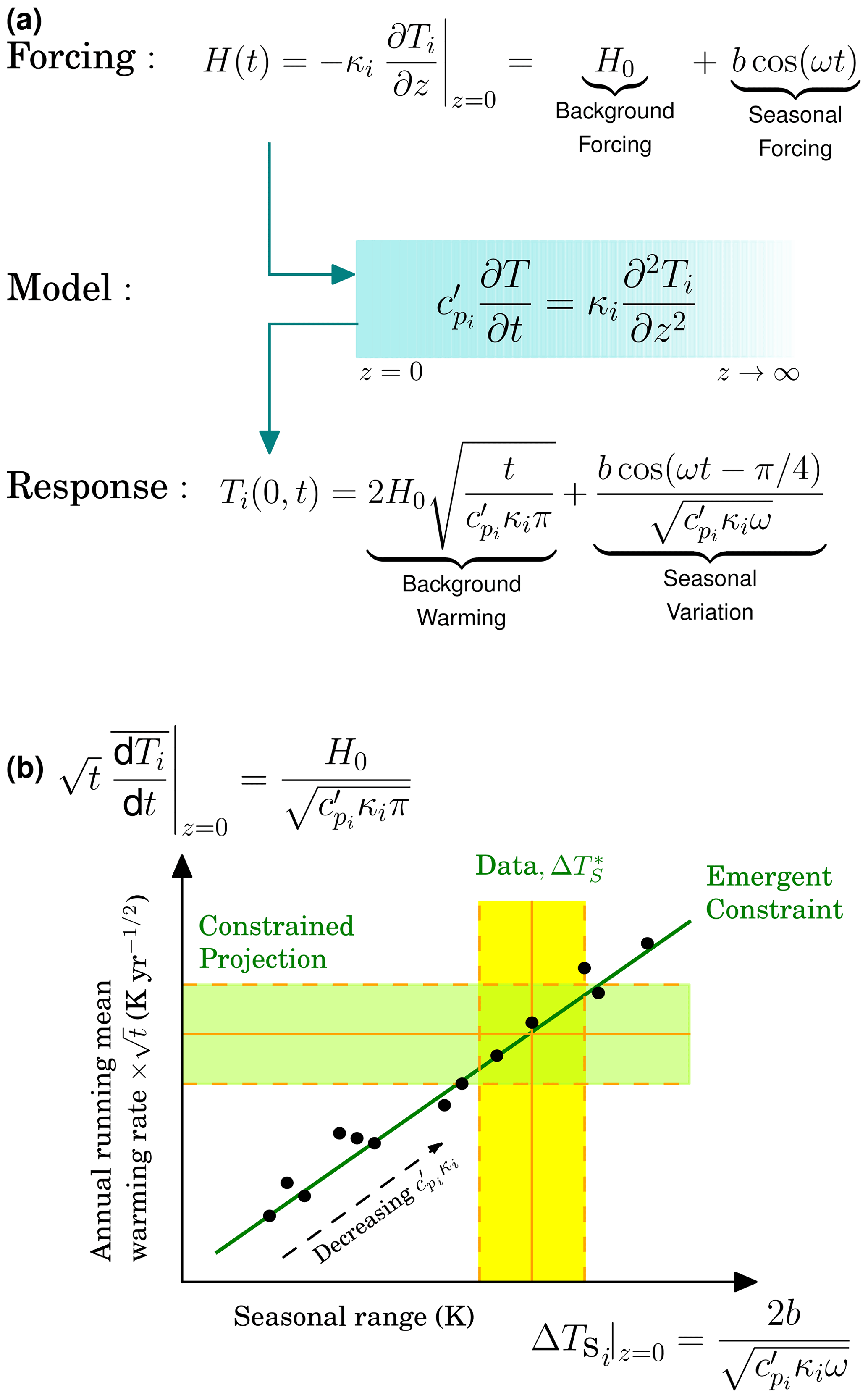
Figure 2 Schematic representation of an emergent constraint with a spatial component. The spatial dimension is defined by variable z. Panel (a) (top row) shows the combined equation for long-term and seasonal forcing at z=0, driving the diffusive model given by Eq. (7) (middle row), and the related response at z=0 and t>0 given by Eqs. (10) and (14) (bottom row). The seasonal forcing (so with ω=2π yr⁻¹) is given by Eq. (8) and the long-term forcing to the thermal model given by Eq. (12). These two forcings generate a response in T at z=0 given by Eqs. (10) and (14) respectively, that combine additively and as shown. Panel (b) illustrates the related emergent constraint based on the response T_i(0,t) shown in (a). This response contains a seasonal (x axis) and long-term (y axis, with seasonality ignored) part, and the EC links the two. The EC allows the observation of seasonal fluctuations, ($\mathrm{\Delta }{T}_{\mathrm{S}}^{*}$, x axis), to constrain the long-term rate of change (y axis). Each model (black dots, indexed by i) has a different implicit value for $c_{p_i}^{\prime }\times {\mathit{\kappa }}_i$. As for the example of Fig. 1, the EC is again assumed to not be exact, with noise causing variation around the regression line. The vertical yellow band represents uncertainty in the measured value of ΔT_S. The constrained projection of the long-term warming rate (multiplied by $\sqrt{t}$, as based on the EC and the value of ΔT_S and its uncertainty), is given by the green horizontal band.

3 Discussion and conclusions

How climate will change due to the ongoing burning of fossil fuels remains one of the highest-profile questions asked of the scientific community. ESMs are central to such research activity, and their primary objective is to predict climate change for different potential future GHG levels as accurately as possible. However, substantial differences can exist between ESM projections, even for the same future scenario of atmospheric GHG changes, so dependable methods are required to reduce the spread in simulations. Emergent constraints are discovered linkages, inter-ESM, between a quantity that is also presently measured and a second important climate attribute associated with future changes, and where data on the former constrain our assessment of the value of the latter. With a constant requirement to provide policymakers with refined estimates of future climate change and against the backdrop of considerable variation between ESMs, ECs have attracted substantial application to a plethora of components of the Earth system. The rapid rise in EC discoveries and their near-ubiquitous use to constrain uncertainty enables a way to extract additional information from available ESMs that have required huge expenditure to build and operate. However, with such a high prominence of ECs as a method to lower uncertainty, it is timely to investigate the assumptions that underline them and any potential pitfalls (e.g. Williamson et al., 2021). Here we start an additional but related route of investigation. We suggest a potential explanation of many ECs is that their basis relates to solving large-scale equations that are implicit in ESMs and have common features between models.

We develop the hypothesis that many identified ECs relate to undiscovered differential equations that describe the Earth system at large geographical scales. Such equations are not coded explicitly in ESMs but instead “emerge” as the aggregation of the finer-resolution behaviour of the climate system. Such finer-resolution features are calculated in ESMs as the solution of differential equations solved on the numerical mesh of each model and capture environmental processes that are often understood well. Such understanding introduces similarities between models, which remain present in any spatial aggregation. The role of ECs is to enable the discovery of the implicit value of parameters associated with such large-scale equations where uncertainty remains. Such bulk parameters affect both a quantity of interest linked to predicting future climate and a contemporary attribute of the Earth system. The contemporary quantity is measurable and, in tandem with the EC, constrains the parameterisation and, thus, understanding of the quantity associated with the future. In many instances of discovered emergent constraints, the present-day component is of a higher-frequency fluctuation (e.g. seasonal), with the EC then used to project a climate attribute of relevance to decadal or century timescales.

We have presented two illustrative examples of solving standard differential equations but placed them in a structure as if they underpin an emergent constraint. We imagine the equations to be underlying large-scale bulk equations, solved implicitly in multiple ESMs, as outlined above. Many examples of equations represent the aggregated behaviour of fine-scale systems. For example, the bulk properties of an ideal gas, temperature and pressure are related through the ideal gas law. However, these bulk properties can also be understood as the aggregated behaviour of the molecules (their mean velocity, mass and number density) that make up the gas. Formally these relations can be made through kinetic theory (Lifshitz and Pitaevskiĭ, 1981). There are also examples of linear bulk dynamics emerging from nonlinear fine-scale dynamics and the converse of effective nonlinear bulk behaviour from linear microscopic dynamics (e.g. the phase transition in the two-dimensional Ising model McCoy and Wu, 1973).

Our first case is a simple box model for which we wish to derive a thermal capacity term, $c_p^{\prime }$, and the second has a single spatial variation and represents a search for a multiplicative combination of capacity and diffusion, $c_p^{\prime }\mathit{\kappa }$. A discovered EC between models, combined with measurements, is in effect revealing the actual real-world value of $c_p^{\prime }$ or $c_p^{\prime }\mathit{\kappa }$. Large values of noise term ϵ_i are for models that are outliers to the EC. In the context of our abstract examples, outliers have different values of effective parameters $c_p^{\prime }$ or $c_p^{\prime }\mathit{\kappa }$ dependent on whether considering shorter seasonal timescales or longer periods, which implies these models have substantially different process representation compared to most other ESMs. We also suggest an additional EC possibility where effective parameters emerge as invariant between ESMs, and instead there is uncertainty in forcings (here, b and H₀, although the uncertainty is similar between the two parameters). Our conceptual model determines internal system properties, i.e. parameters, which for the spatial example are constrained based on behaviours at the edges of the domain. We note the basic theorems of vector calculus (e.g. Stokes' theorem) that relate integrated internal system features to conditions along domain edges.

A broad set of possibilities may link to our suggestion that the underlying principle of many ECs is the existence of equations valid at large scales. For instance, in addition to our example of diffusion, ECs may reveal implicit PDEs with an advective component corresponding to atmospheric transport. In many cases, atmospheric transport provides the coupling between two spatially distant components of the Earth system, generating what is often called a “teleconnection”. To constrain the strength of future teleconnections, an EC is likely to need a present-day measurement of wind fluxes or measurements of a quantity of interest in two locations. In addition, modelling many components of the Earth system requires coupled differential equations to link different physical quantities and capture changes of state, where geochemical cycles link tightly to climate variation. An example of an EC capturing features of a coupled system is that of Cox et al. (2013). In that analysis, data on present-day simultaneous fluctuations in atmospheric CO₂ and annual temperature anomalies reveal the fate of future South American carbon stores under global warming and the related risk of Amazon forest “die-back”. In some cases, the EC x axis, for which measurements exist, is a combination of high-frequency drivers and response, and for the same variable. As an example of such a more refined and complex contemporary statistic, Cox et al. (2018) estimate equilibrium climate sensitivity with a statistic Ψ that is a combination of the standard deviation and autocorrelation of current global temperature fluctuations. Arguably, the Ψ statistic merges a system driver (standard deviation) and a response (autocorrelation). Here, we assume underlying PDEs that are simple by design to aid transparency. Making these underlying models more relevant to the Earth's climate is an outstanding challenge. Additional to horizontal heat transport, our planet emits longwave radiation to the wider universe. Such radiation provides the restoring force, λ, that ultimately stabilises the near-surface temperature. Including such a restoring force in our simple PDE models is one possible extension of our analysis, although, in tandem with an unknown heat capacity, c_p, this would potentially generate a two-dimensional EC. In practice, fitting a two-dimensional EC may be challenging given the relatively small number of data points (i.e. available ESMs). Analytical solutions may exist that allow for a time-varying value of H₀ that approximates known historical climatic forcing.

In summary, the analysis of ensembles of ESMs, as built by different research centres, has revealed multiple emergent constraints for all parts of the Earth system (Hall et al., 2019). Discovered ECs have reduced uncertainty bounds for features of the climate system that directly affect society and are, therefore, of particular interest to policymakers. With the placement of much emphasis on the EC method to lower uncertainty, there is a growing requirement to understand its underlying assumptions better. Timely research is emerging that critically assesses the method (e.g. Williamson et al., 2021). We add to the discussion by suggesting that many ECs represent the discovery of parameters associated with large-scale implicit equations that describe features of the Earth system. Such equations emerge from the aggregation of more local effects simulated on the grid points of the numerical meshes of individual ESMs. With the prevailing view that physical intuition should guide EC discoveries rather than, e.g. data mining, our suggestion supports that standpoint. Hence we consider most ECs to correspond to underlying processes and related mathematical representation. This bulk process discovery helps counter a view that ESMs are so complex that they can never be amenable to interpretation via standard applied mathematics techniques (a concern raised by Huntingford, 2017). Such methods include scaling of the equations directly coded in ESMs (“nondimensionalisation”) to find the dominant underlying forms, although we speculate that EC discovery may instead identify key large-scale processes. Further hinting at the need to confirm underlying processes is the analysis of Qu et al. (2018). Those authors consider the statistical linkages between four different ECs proposed for ECS and suggest that the discovered commonalities are because each is constraining, implicitly, shortwave radiation cloud feedbacks. We present two simple illustrative examples of differential equations, their solutions, and their potential interpretation as ECs. Despite differential equations representing a range of processes, mathematics can often characterise them in discrete ways (for instance, every linear second-order PDE being either diffusive, elliptic or hyperbolic). The perspective offered here may open ways to classify ECs based on the type of any discovered underpinning equations they link to. Confirming such links allows the study of some aspects of climate change from a more analytical applied mathematics standpoint. The equation forms may be PDEs, they may be coupled, or they could be simply ordinary differential equations or in algebraic form. Although our examples are synthetic, we hope the concepts we present support the placement of ECs on a stronger theoretical footing by, where applicable, revealing underlying bulk equations that fit with process intuition. Brient (2020) argues that when multiple ECs exist to predict the same quantity, each should be weighted by the level of physical understanding they offer to elucidate the relationship. It remains important to understand ECs as they offer an elegant potential capability to lower the continuing uncertainty between ESM projections. In conclusion, we suggest an interpretation of ECs is that they reveal parameters of large-scale implicit differential equations that aggregate the numerical finite differencing upon which ESMs are built.