Understanding variations in downwelling longwave radiation using Brutsaert's equation

A dominant term in the surface energy balance and central to global warming is downwelling longwave radiation (R_ld). It is influenced by radiative properties of the atmospheric column, in particular by greenhouse gases, water vapor, clouds, and differences in atmospheric heat storage. We use the semi-empirical equation derived by Brutsaert (1975) to identify the leading terms responsible for the spatial–temporal climatological variations in R_ld. This equation requires only near-surface observations of air temperature and humidity. We first evaluated this equation and its extension by Crawford and Duchon (1999) with observations from FLUXNET, the NASA-CERES dataset, and the ERA5 reanalysis. We found a strong spatiotemporal correlation between estimated R_ld and the datasets above, with r² ranging from 0.87 to 0.98 across the datasets for clear-sky and all-sky conditions. We then used the equations to show that changes in lower atmospheric heat storage explain more than 95 % and around 73 % of diurnal range and seasonal variations in R_ld, respectively, with the regional contribution decreasing with latitude. Seasonal changes in the emissivity of the atmosphere play a second role, which is controlled by anomalies in cloud cover at high latitudes but dominated by water vapor changes at midlatitudes and subtropics, especially over monsoon regions. We also found that as aridity increases over the region, the contributions from changes in emissivity and lower atmospheric heat storage tend to offset each other (−40 and 20–30 W m⁻², respectively), explaining the relatively small decrease in R_ld with aridity (−(10–20) W m⁻²). These equations thus provide a solid physical basis for understanding the spatiotemporal variability of surface downwelling longwave radiation. This should help us to better understand and interpret climatological changes, such as those associated with extreme events and global warming.

1 Introduction

In the global mean surface energy budget, downward longwave radiation (R_ld) is dominant surface energy input (333 W m⁻² in global mean and 306 W m⁻² over land), contributing around twice as much energy as absorbed solar radiation (161 W m⁻² in global mean and 184 W m⁻² over land) (Trenberth et al., 2009; Wild et al., 2015). This dominance holds over all regions in the climatological mean, although there are some clear variations in space and time (Figs. 1 and S1). It is central to global warming, reflecting the greenhouse effect of the atmosphere (Held and Soden, 2000), and its variations have been suggested to be the main contributor to some regional warming amplifications, such as in the Arctic (Lee et al., 2017) and the Tibetan Plateau (Su et al., 2017). Therefore, it is important to understand the main sources of variations in this surface energy balance term, which can be seen in Fig. 1.

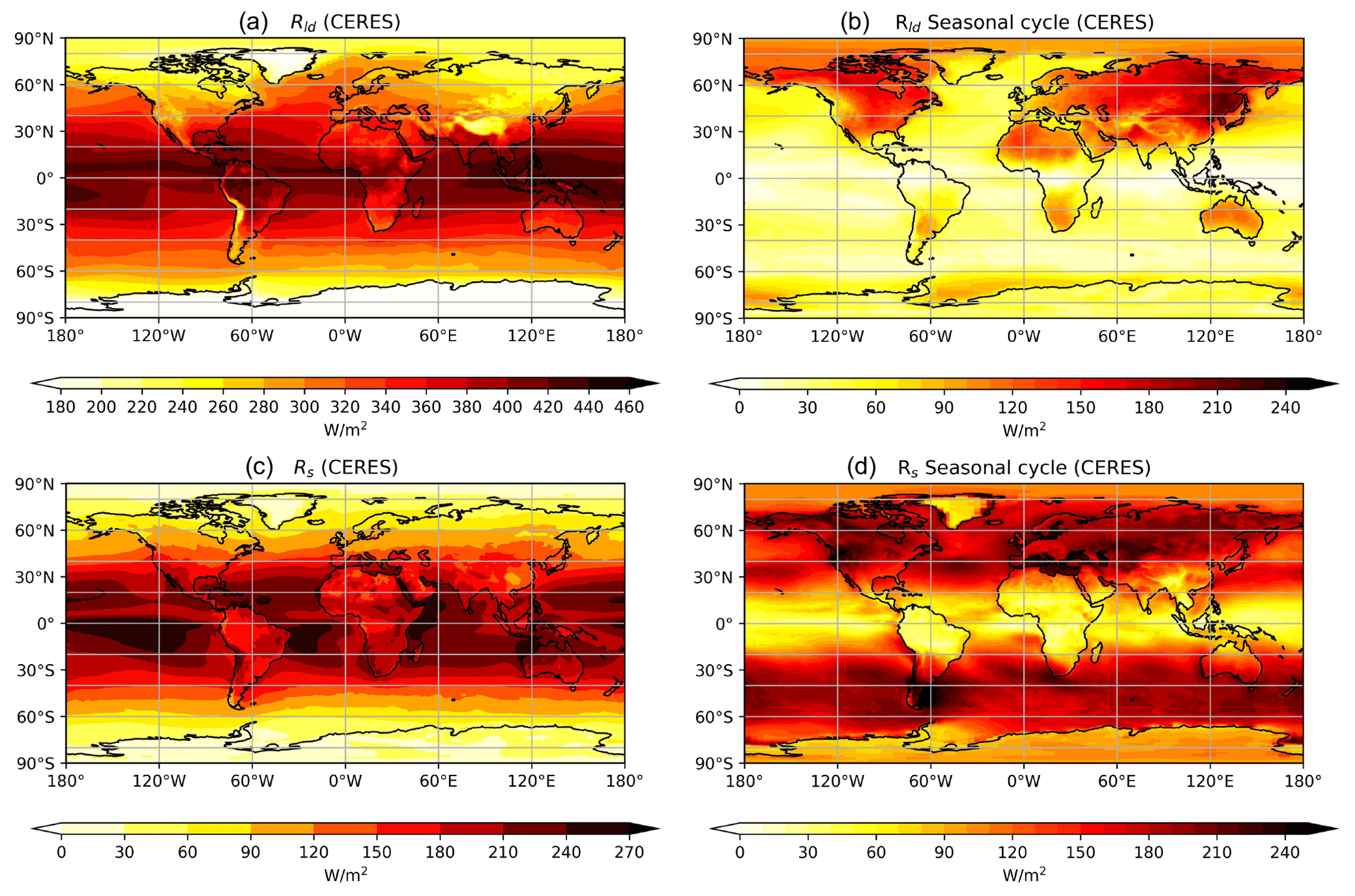
Figure 1 Spatial distribution of (a, c) the climatological mean and (b, d) the seasonal amplitude of downward longwave radiation and absorbed solar radiation at the surface, respectively, from the NASA-CERES dataset. The seasonal amplitude is calculated as the difference between the maximum and minimum monthly data.

The flux of downwelling longwave radiation is influenced by the radiative properties of the entire atmospheric column, i.e., water vapor, clouds, and greenhouse gases, but also by the heat stored in the atmosphere, i.e., the temperature at which radiation is emitted back to the surface. To obtain an estimate of this flux, Brutsaert (1975) used functional expressions for the typical temperature and humidity profiles of the lower troposphere together with radiative transfer equations and semiempirical relationships of the absorptivity by water vapor, integrated these vertically, and expressed the resulting flux R_ld in terms of near-surface air temperature and water vapor pressure for clear-sky conditions. He thereby derived a semi-empirical equation for R_ld for an effective clear-sky emissivity (ε_cs) and the corresponding flux of downwelling longwave radiation (R_ld,cs):

$$\begin{array}{}\text{(1)}& {\displaystyle }{\mathit{\epsilon }}_{\mathrm{cs}}=\mathrm{1.24}{\left(e_{\mathrm{a}}/T_{\mathrm{a}}\right)}^{\mathrm{1}/\mathrm{7}},\text{(2)}& {\displaystyle }{R}_{\mathrm{ld},\mathrm{cs}}={\mathit{\epsilon }}_{\mathrm{cs}}\mathit{\sigma }{T}_{\mathrm{a}}^{\mathrm{4}},\end{array}$$

where σ is the Stefan–Boltzmann constant ($\mathit{\sigma }=\mathrm{5.67}\times {\mathrm{10}}^{-\mathrm{8}}$ W m⁻² K⁻⁴), e_a is the 2 m water vapor pressure (unit: mbar) and T_a is the 2 m air temperature (unit: K). The latter two meteorological variables can easily be obtained or inferred from weather stations, meaning that the downwelling flux of longwave radiation can be estimated from weather station observations. Note that the ε_cs shown in Eq. (1) is largely insensitive to changes in T_a. As a result, emissivity does not have a direct dependence on T_a, except that higher temperature may also lead to higher values in e_a.

This equation was later extended to all-sky conditions that include the effects of cloud cover, among which Crawford and Duchon (1999) is a common extension (Alados et al., 2012; Duarte et al., 2006; Flerchinger et al., 2009). This extension diagnoses cloud cover fraction (f_c) as the fraction of incoming solar radiation at the surface (R_s) in relation to the potential solar radiation (R_s,pot), that is, the incoming flux at the top of the atmosphere. The emissivity for all-sky conditions, ε, is then calculated as the mix of the emissivities of clear-sky conditions (Eq. 1) (weighted by the cloud-free proportion, i.e., 1−f_c) and clouds with an emissivity of ε_c= 1 (weighted by the cloud fraction f_c). Using this emissivity, the estimation of downwelling longwave radiation is then done by

$$\begin{array}{}\text{(3)}& {\displaystyle }{f}_{\mathrm{c}}=\mathrm{1}-R_{\mathrm{s}}/R_{\mathrm{s},\mathrm{pot}},\text{(4)}& {\displaystyle }\mathit{\epsilon }=f_{\mathrm{c}}+\left(\mathrm{1}-f_{\mathrm{c}}\right){\mathit{\epsilon }}_{\mathrm{cs}},\text{(5)}& {\displaystyle }{R}_{\mathrm{ld}}=\mathit{\epsilon }\mathit{\sigma }{T}_{\mathrm{a}}^{\mathrm{4}}.\end{array}$$

Previous studies have already verified Eqs. (4)–(5) to have a very good agreement with site measurements with the r² of 0.883 and RMSE of 15.367 W m⁻² (Duarte et al., 2006; Hatfield et al., 1983), especially when the temperature is higher than 0^∘ (Aase and Idso, 1978; Satterlund, 1979). Other studies have worked to calibrate and modify this estimate further to different regions (Malek, 1997; Sridhar and Elliott, 2002).

This expression for downwelling longwave radiation R_ld given by Eq. (5) allows us to quantify the different contributions by cloud cover, f_c; water vapor concentrations, e_a (as a measure of the total water vapor content of the atmospheric column); and air temperature, T_a (as a proxy for the heat storage within the lower atmosphere, Panwar et al., 2022). With this, we can then attribute variations in R_ld to their physical causes.

Here, our aim is to first evaluate this estimate for downwelling longwave radiation with current global datasets at the continental scale. These variations are illustrated using the NASA-CERES (EBAF 4.1) dataset (Loeb et al., 2018; Kato et al., 2018; NASA/LARC/SD/ASDC, 2017) and the NASA-CERES Syn1deg dataset (Doelling et al., 2013, 2016) in Fig. 1 and are compared to variations in solar radiation. It can be seen that the climatological distribution of R_ld is mostly associated with latitudes, while also presenting some zonal variations, e.g., across western and eastern North America. In comparison, the seasonal cycle of R_ld is less determined by latitudes (Fig. 1b). It has a larger magnitude over land than over oceans, over arid regions than humid regions, and over cold regions more than over warm ones. Although studies have revealed a close correlation between the variation of R_ld and other factors like air temperature, water vapor, and CO₂ concentration (Wang and Liang, 2009; Wei et al., 2021), here we go beyond correlations and instead attribute these variations to the different terms in Eqs. (1)–(5) that represent different radiative properties affecting R_ld.

To figure out the dominant driver for these spatiotemporal variations, we decompose changes in R_ld into its components: cloud cover, f_c; heat storage changes of atmosphere as reflected by 2 m air temperature, T_a; and air humidity, e_a, by performing the differentiation of these equations. We show that heat storage changes predominantly shape the diurnal range and seasonal cycle of R_ld, while cloud cover variations play a second role in most cases. In addition, the temporal variations of R_ld are lower over the ocean than over land and lower during winter than summer. On the other hand, the spatial variations of R_ld from arid to humid regions is relatively small, which we will show is due to a compensating effect of corresponding changes in atmospheric emissivity and heat storage.

Our paper is organized as follows. After briefly describing the datasets used in our evaluation in Sect. 2, we first the estimate of R_ld from these equations at the global scale using multiple datasets in Sect. 3.1. After showing that the annual mean and large-scale variations are well captured, we then use the equations to decompose the temporal variations of R_ld in terms of its mean spatial and temporal variations and relate these to their causes in Sect. 3.2. The spatial variations of R_ld are then further discussed in Sect. 3.3 in terms of their relationship with aridity. We then close with a brief summary and broader implications.

2 Datasets

To test R_ld estimates, we use FLUXNET 30 min observations (Pastorello et al., 2020, 30 min values, 189 sites; see Table S1 and Fig. S2 for details), the NASA-CERES monthly satellite-based radiation dataset (Doelling et al., 2013, 2016, monthly means, covering years 2001 to 2018), and the ERA5 monthly reanalysis dataset (Hersbach et al., 2022, monthly means, covering years 1979 to 2021).

For each dataset, T_a, e_a, and f_c are needed as inputs for Eqs. (1)–(5), while R_ld data are used for the comparison. Cloud cover f_c is calculated using Eq. (3) for all three datasets with incoming solar radiation at the surface (R_s) and the potential solar radiation (R_s,pot). For NASA-CERES estimation, T_a from the CPC Global Unified Temperature dataset (CPC Global Unified Temperature, 2022) is used as temperature observation.

For all three datasets, water vapor pressure, e_a, is not directly given. It is calculated from the water vapor deficit (VPD, FLUXNET) or dew-point temperature (T_dew, ERA5) using Monteith and Unsworth (2008):

$$\begin{array}{}\text{(6)}& {\displaystyle }{e}_{\mathrm{a}}=\mathrm{6.1079}\times \exp \left(\mathrm{17.269}{T}_{\mathrm{dew}}/\left(\mathrm{237.3}+T_{\mathrm{dew}}\right)\right),\text{(7)}& {\displaystyle }{e}_{\mathrm{a}}=\mathrm{6.1079}\times \exp \left(\mathrm{17.269}{T}_{\mathrm{a}}/\left(\mathrm{237.3}+T_{\mathrm{a}}\right)\right)-\mathrm{VPD},\end{array}$$

and the calculated e_a from ERA5 is also used in NASA-CERES estimation.

For the analysis of the spatial variations of R_ld along water availability, we use the aridity index ($\mathrm{AI}=\frac{R}{\mathrm{LP}}$) (Budyko, 1958; UNCOD, 1977). This index is calculated using the mean annual net radiation (R) taken from the NASA-CERES dataset, the mean annual net precipitation (P) taken from the CPC Global Unified Gauge-Based Analysis of Daily Precipitation data (Chen et al., 2008; Xie et al., 2007; CPC Global Unified Gauge-Based Analysis of Daily Precipitation, 2022), and a latent heat of vaporization for water of L=2260 kJ kg⁻¹. A larger value of AI indicates stronger aridity.

3 Results and discussion

3.1 Comparison to observed, satellite, and reanalysis data

We first compared the estimates of R_ld at a point-by-point basis separately for clear-sky and all-sky conditions using Eqs. (2) and (5), respectively. This comparison is shown in Fig. 2 using FLUXNET, CERES, and ERA5 data. The estimates correlate very well with r² of 0.92 and 0.87 for clear-sky and all-sky conditions, respectively, and RMSE values of 18.24 and 24.56 W m⁻². The slope of the linear regressions between the estimated and observed R_ld for FLUXNET are 1.03 and 1.02, with most data points being concentrated around the 1:1 line (Fig. 2a and b). Note that for all-sky conditions the agreement is slightly less good, with a lower correlation coefficient and a larger RMSE. The agreement with the NASA-CERES and ERA5 datasets are even better, with higher correlation coefficients and lower RMSE.

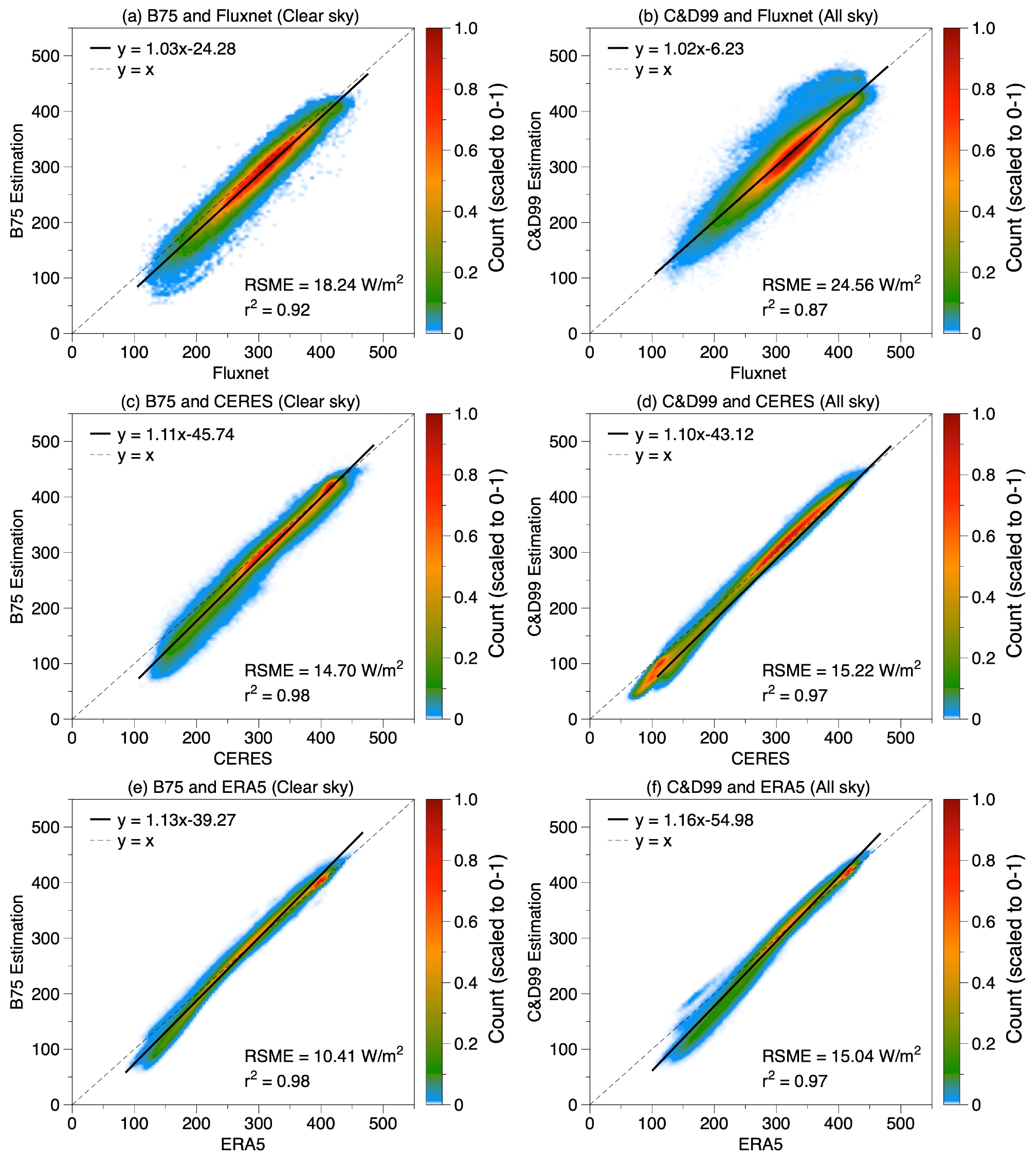
Figure 2 Comparison of R_ld estimated by Brutsaert (1975) (a, c, e) for clear-sky conditions and by Crawford and Duchon (1999) (b, d, f) for all-sky conditions using (a, b) FLUXNET hourly data of 189 sites, (c, d) NASA-CERES monthly data of $\mathrm{1}{}^{\circ }\times \mathrm{1}{}^{\circ }$ from 2001–2018, and (e, f) ERA5 monthly data of resolution of $\mathrm{1}{}^{\circ }\times \mathrm{1}{}^{\circ }$ from 1979–2021. Colors indicate the density of the data points and are scaled to values between 0–1.

Despite this high level of agreement of the estimates, we can see some systematic biases in the estimates for R_ld. These can be seen in Figs. 3 and S3, which show the spatial distribution of these biases and their variations against temperature and humidity. For clear-sky conditions, there appears to be a general underestimation in the high latitudes and, to some extent, in arid regions (Fig. 3c and e). Brutsaert  (1975) already described that for very low temperatures and in arid conditions, there are better parameter values than those used in Eq. (1), with a larger coefficient than 1.24 and a different exponent. This can then lead to an underestimation of R_ld under low humidity (Figs. 3b, S3b, S3d). Moreover, B75 has not considered the gradual increase in emissivity as temperature decreases below freezing (Aase and Idso, 1978), thus explaining the underestimation under low temperature (Figs. 3b, S3a, S3c). The biases seen in Fig. 3 are nevertheless notably smaller than the spatial–temporal variations shown in Fig. 1. This means that these biases do not prevent us from using Brutsaert to attribute the causes for the seasonal variation and the spatial range of R_ld.

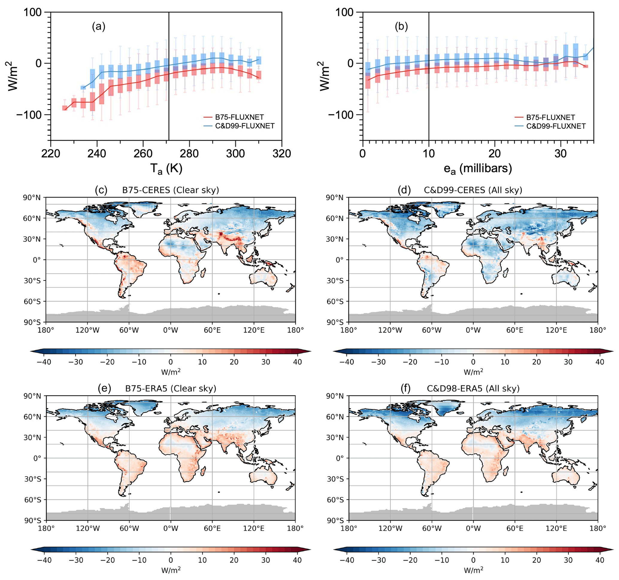
Figure 3 Biases in the estimates for multi-year mean R_ld for FLUXNET data of 189 sites against (a) air temperature and (b) water vapor pressure. Distribution of biases in the estimates for multi-year mean R_ld for (c, d) NASA-CERES data from 2001–2018 and (e, f) ERA reanalysis from 1979–2021 for (c, e) clear-sky and (d, f) all-sky conditions over land. Grey shading indicates missing values.

The biases for all-sky conditions generally share the distribution with that of clear-sky conditions, with a smaller magnitude (Fig. 3b, d and f), which are also small compared to the spatial–temporal variations.

Overall, this evaluation shows that the expressions given by Eqs. (1)–(5) are very well suited to describe the spatiotemporal variations of R_ld for current climatological conditions.

3.2 Attribution of diurnal and seasonal variations

We next use Eqs. (1)–(5) to attribute temporal variations of R_ld to their physical causes. To do so, we can express changes ΔR_ld as a function of changes in water vapor, Δe_a; cloud cover, Δf_c; and air temperature, ΔT_a. The functional dependence is derived from the equations by differentiation and applying the chain rule. In a first step, we express a change ΔR_ld by the partial contributions ΔR_ld,ε and ΔR_ld,T that is due to changes in emissivity, Δε, and due to changes in atmospheric heat storage that are associated with a change in air temperature ΔT_a:

$$\begin{array}{}\text{(8)}& \begin{array}{rl}\mathrm{\Delta }{R}_{\mathrm{ld}}& =\mathrm{\Delta }{R}_{\mathrm{ld},\mathit{\epsilon }}+\mathrm{\Delta }{R}_{\mathrm{ld},T}={\displaystyle \frac{\partial R_{\mathrm{ld}}}{\partial \mathit{\epsilon }}}\mathrm{\Delta }\mathit{\epsilon }+{\displaystyle \frac{\partial R_{\mathrm{ld}}}{\partial T_{\mathrm{a}}}}\mathrm{\Delta }{T}_{\mathrm{a}}\\ & =\mathit{\sigma }{\stackrel{\mathrm{‾}}{T_{\mathrm{a}}}}^{\mathrm{4}}\mathrm{\Delta }\mathit{\epsilon }+\mathrm{4}\mathit{\sigma }\stackrel{\mathrm{‾}}{\mathit{\epsilon }}{\stackrel{\mathrm{‾}}{T_{\mathrm{a}}}}^{\mathrm{3}}\mathrm{\Delta }{T}_{\mathrm{a}}.\end{array}\end{array}$$

The two terms on the right side of Eq. (8) are ΔR_ld,ε and ΔR_ld,T, respectively.

The contribution ΔR_ld,ε is further decomposed into contributions $\mathrm{\Delta }{R}_{\mathrm{ld},f_{\mathrm{c}}}$, $\mathrm{\Delta }{R}_{\mathrm{ld},e_{\mathrm{a}}}$, and $\mathrm{\Delta }{R}_{\mathrm{ld},T_{\mathrm{a}}^{\prime }}$ due to variations in clouds, Δf_c, air humidity, Δe_a, and surface temperature, ΔT_a, and we obtain the following equation:

$$\begin{array}{}\text{(9)}& \begin{array}{rl}\mathrm{\Delta }{R}_{\mathrm{ld},\mathit{\epsilon }}& =\mathit{\sigma }{\stackrel{\mathrm{‾}}{T_{\mathrm{a}}}}^{\mathrm{4}}\mathrm{\Delta }\mathit{\epsilon }\approx \mathit{\sigma }{\stackrel{\mathrm{‾}}{T_{\mathrm{a}}}}^{\mathrm{4}}\times {\displaystyle \frac{\partial \mathit{\epsilon }}{\partial f_{\mathrm{c}}}}\mathrm{\Delta }{f}_{\mathrm{c}}+\mathit{\sigma }{\stackrel{\mathrm{‾}}{T_{\mathrm{a}}}}^{\mathrm{4}}\\ & \times {\displaystyle \frac{\partial \mathit{\epsilon }}{\partial e_{\mathrm{a}}}}\mathrm{\Delta }{e}_{\mathrm{a}}+\mathit{\sigma }{\stackrel{\mathrm{‾}}{T_{\mathrm{a}}}}^{\mathrm{4}}\times {\displaystyle \frac{\partial \mathit{\epsilon }}{\partial T_{\mathrm{a}}}}\mathrm{\Delta }{T}_{\mathrm{a}}=\mathit{\sigma }{\stackrel{\mathrm{‾}}{T_{\mathrm{a}}}}^{\mathrm{4}}\\ & \times \left(\mathrm{1}-\stackrel{\mathrm{‾}}{\mathrm{1.24}{\left({\displaystyle \frac{\stackrel{\mathrm{‾}}{e_{\mathrm{a}}}}{\stackrel{\mathrm{‾}}{T_{\mathrm{a}}}}}\right)}^{\frac{\mathrm{1}}{\mathrm{7}}}}\right)\mathrm{\Delta }{f}_{\mathrm{c}}+\mathit{\sigma }{\stackrel{\mathrm{‾}}{T_{\mathrm{a}}}}^{\mathrm{4}}\\ & \times {\displaystyle \frac{\mathrm{1.24}}{\mathrm{7}}}{\displaystyle \frac{\left(\mathrm{1}-\stackrel{\mathrm{‾}}{f_{\mathrm{c}}}\right)}{{\left(\stackrel{\mathrm{‾}}{e_{\mathrm{a}}}\right)}^{\frac{\mathrm{6}}{\mathrm{7}}}{\left(\stackrel{\mathrm{‾}}{T_{\mathrm{a}}}\right)}^{\frac{\mathrm{1}}{\mathrm{7}}}}}\mathrm{\Delta }{e}_{\mathrm{a}}+\mathit{\sigma }{\stackrel{\mathrm{‾}}{T_{\mathrm{a}}}}^{\mathrm{4}}\times \left(-{\displaystyle \frac{\mathrm{1.24}}{\mathrm{7}}}\right)\\ & \times {\displaystyle \frac{\left(\mathrm{1}-\stackrel{\mathrm{‾}}{f_{\mathrm{c}}}\right){\left(\stackrel{\mathrm{‾}}{e_{\mathrm{a}}}\right)}^{\frac{\mathrm{1}}{\mathrm{7}}}}{{\left(\stackrel{\mathrm{‾}}{T_{\mathrm{a}}}\right)}^{\frac{\mathrm{8}}{\mathrm{7}}}}}\times \mathrm{\Delta }{T}_{\mathrm{a}}.\end{array}\end{array}$$

The three terms on the right side of Eq. (9) are $\mathrm{\Delta }{R}_{\mathrm{ld},f_{\mathrm{c}}}$, $\mathrm{\Delta }{R}_{\mathrm{ld},e_{\mathrm{a}}}$, and $\mathrm{\Delta }{R}_{\mathrm{ld},T_{\mathrm{a}}^{\prime }}$.

Note that the third term is of lower magnitude compared with the other two terms (e.g., in terms of the seasonal range as shown in Fig. 5f), which is hence not focused on in this work.

We next applied this approach to the diurnal deviations ΔR_ld from the daily mean using the FLUXNET dataset. This decomposition is shown in Fig. 4 in aggregated form across the FLUXNET sites for the whole year (Fig. 4a) and the Northern Hemisphere summer (Fig. 4b) and winter seasons (Fig. 4c). More than 95 % of the diurnal variations (of about ± 20 W m⁻²) are caused by diurnal changes in air temperature, while variations in emissivity play practically no role (Fig. S4). Diurnal changes in air temperature reflect variations in heat storage of the atmospheric boundary layer. This is consistent with the notion that diurnal variations in solar radiation over land are buffered primarily by the lower atmosphere, rather than below the surface as is the case for open water bodies and the ocean (Kleidon and Renner, 2017). Since most of the stations in the FLUXNET dataset are located in the midlatitudes of the Northern Hemisphere, the variations are consistently larger in summer due to the greater solar input (Fig. 4b) than in winter (Fig. 4c).

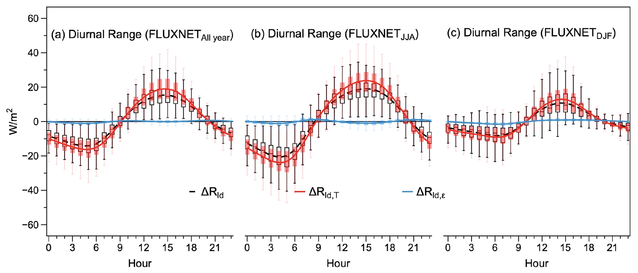
Figure 4 The multi-year average diurnal variations in R_ld (dashed black line) and its decomposition into contributions by changes in emissivity (blue, ΔR_ld,ε) and lower atmospheric heat storage (red, ΔR_ld,T) in the FLUXNET dataset aggregated over 189 sites for (a) the whole year, (b) June–August, and (c) December–February. The box shows the variation among the 189 sites. The upper and lower whiskers indicate the 95th and 5th percentiles, respectively, while the upper boundary, median line, and lower boundary of the box indicate the 75th, 50th, and 25th quantiles, respectively. For each site and each day, the daily mean value is removed, with the deviations shown. Regression lines are based on site-mean or grid-mean value using LOESS regression.

Figure 5 shows the same kind of decomposition, but for seasonal variations in R_ld in the NASA-CERES dataset, which is the difference between the maximum and minimum of monthly R_ld data. Generally, areas with relatively low annual-mean R_ld, e.g., the high-latitude regions of North America and northeastern Eurasia, have the largest seasonal cycle (Fig. 1). The decomposition shows that this variation is mostly due to the seasonal variation in atmospheric heat storage (ΔR_ld,T), with a portion of around 73 % on a global scale, and the rest are attributed to the seasonal changes in water vapor (24 %) and cloud cover (12 %). Notably, seasonal variations in emissivity play a greater role than atmospheric heat storage in changing R_ld in tropical areas, especially over the monsoon region. This is predominantly due to the strong seasonal fluctuations in water vapor levels and cloud cover (Fig. 5d–f).

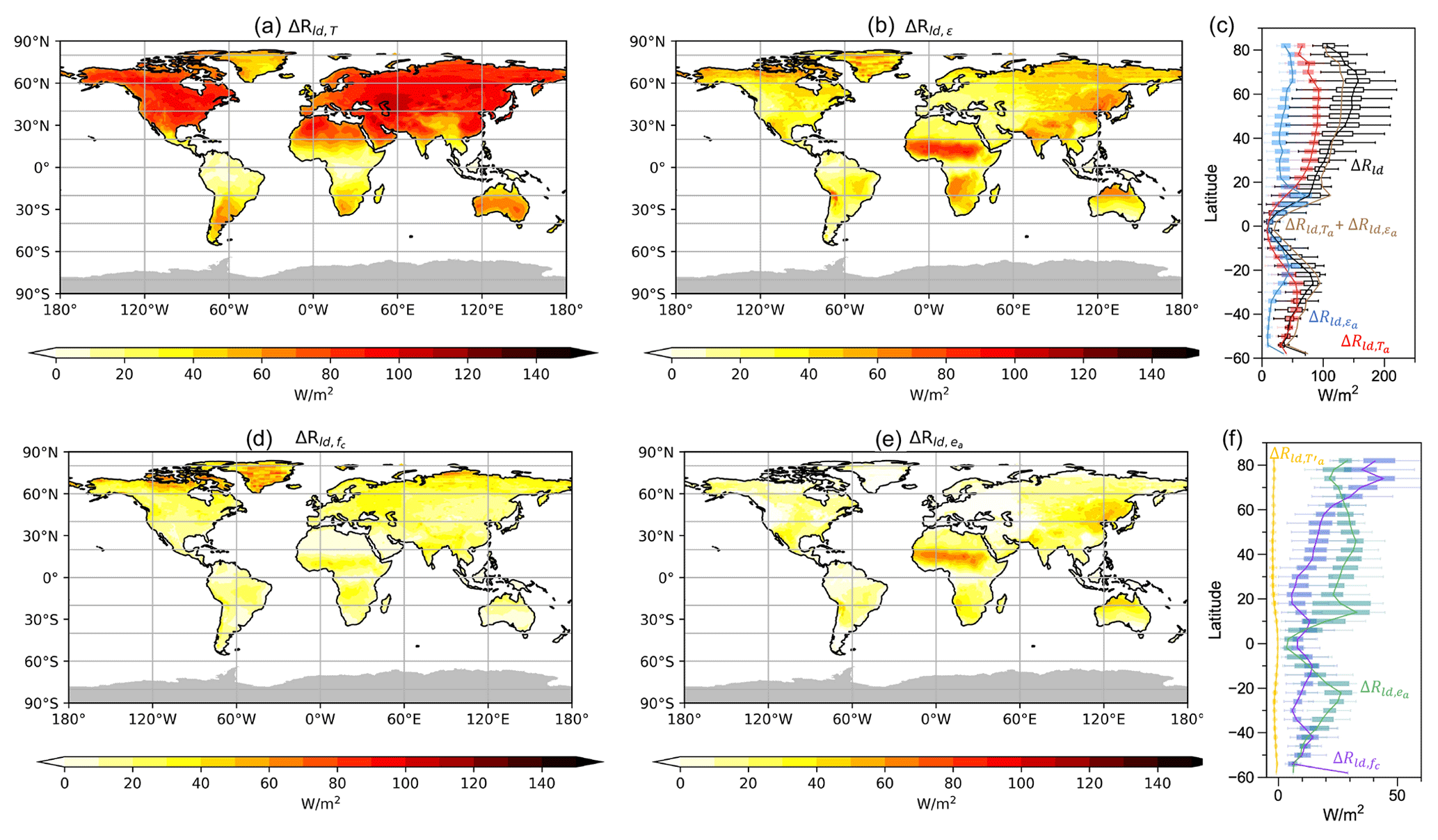
Figure 5 Decompositions of the mean seasonal variation (Δ, difference between the maximum and minimum monthly data at each grid) of R_ld in the NASA-CERES dataset into contributions by (a) lower atmospheric heat storage (ΔR_ld,T) and (b) emissivity (ΔR_ld,ε) and (c) their latitudinal variations. Decomposition of ΔR_ld,ε into contributions by variations in (d) cloud cover ($\mathrm{\Delta }{R}_{\mathrm{ld},f_{\mathrm{c}}}$), (e) humidity ($\mathrm{\Delta }{R}_{\mathrm{ld},e_{\mathrm{a}}}$), and (f) their latitudinal variations. In (a), (b), (d), and (e), grey shading indicates missing values. In (c) and (f), the box shows the variation among the land grids at the same latitude, while the solid line is their mean. The upper and lower whiskers indicate the 95th and 5th percentiles, respectively, while the upper boundary, median line, and lower boundary of the box indicate the 75th, 50th, and 25th quantiles, respectively.

The aggregation to the global scale across land and ocean is shown in Fig. S5, where the deviations are calculated as the difference in the monthly means to the annual mean. Figure S5 show that the seasonal variations of R_ld are generally lower over the ocean than on the land, an effect that can also be seen in Fig. 1. The decomposition shows that these variations are mostly caused by changes in lower atmospheric heat storage, with a slight modulation by emissivity changes. This can, again, be largely explained by the effect described above for the diurnal variations (Kleidon and Renner, 2017). Over the land, the changes in radiation are majorly buffered by the heat storage in the lower atmosphere and the variations in convective boundary layer height. However, over marine areas, solar radiation penetrates the transparent water bodies, the heat storage of which buffers the season cycle of the radiation over the ocean. Since the heat storage of the water body is larger than that of the lower atmospheric boundary layer, the buffering effect is consequently larger, which leads to the less severe seasonal cycle of surface temperature and R_ld over the ocean.

In summary, what our decomposition shows is that most temporal variations in R_ld in current climatological conditions are explained by heat storage changes within the lower atmosphere.

3.3 Attribution of geographic variations with aridity

Last, we applied the decomposition to the climatological variations in R_ld along with differences in mean water availability. Water availability was characterized by Budyko's aridity index (AI), with values AI < 1 representing humid regions, and larger values reflecting increased aridity. The spatial distribution of AI is shown in Fig. S6. Here, the deviations ΔR_ld are calculated with respect to the annual mean over land. The different contributions to the deviations are shown in Fig. 6, as well as the delineation along the aridity index (Fig. 6e–f).

The decomposition of the spatial distribution of the climatological means shows that the variations are largely caused by differences in lower atmospheric heat storage as well (Fig. 6a). The contribution due to variations in emissivity has a smaller magnitude (Fig. 6b) and is dominated by changes in cloud cover (Fig. 6c) and changes in water vapor (Fig. 6d) at high latitudes and midlatitudes, respectively.

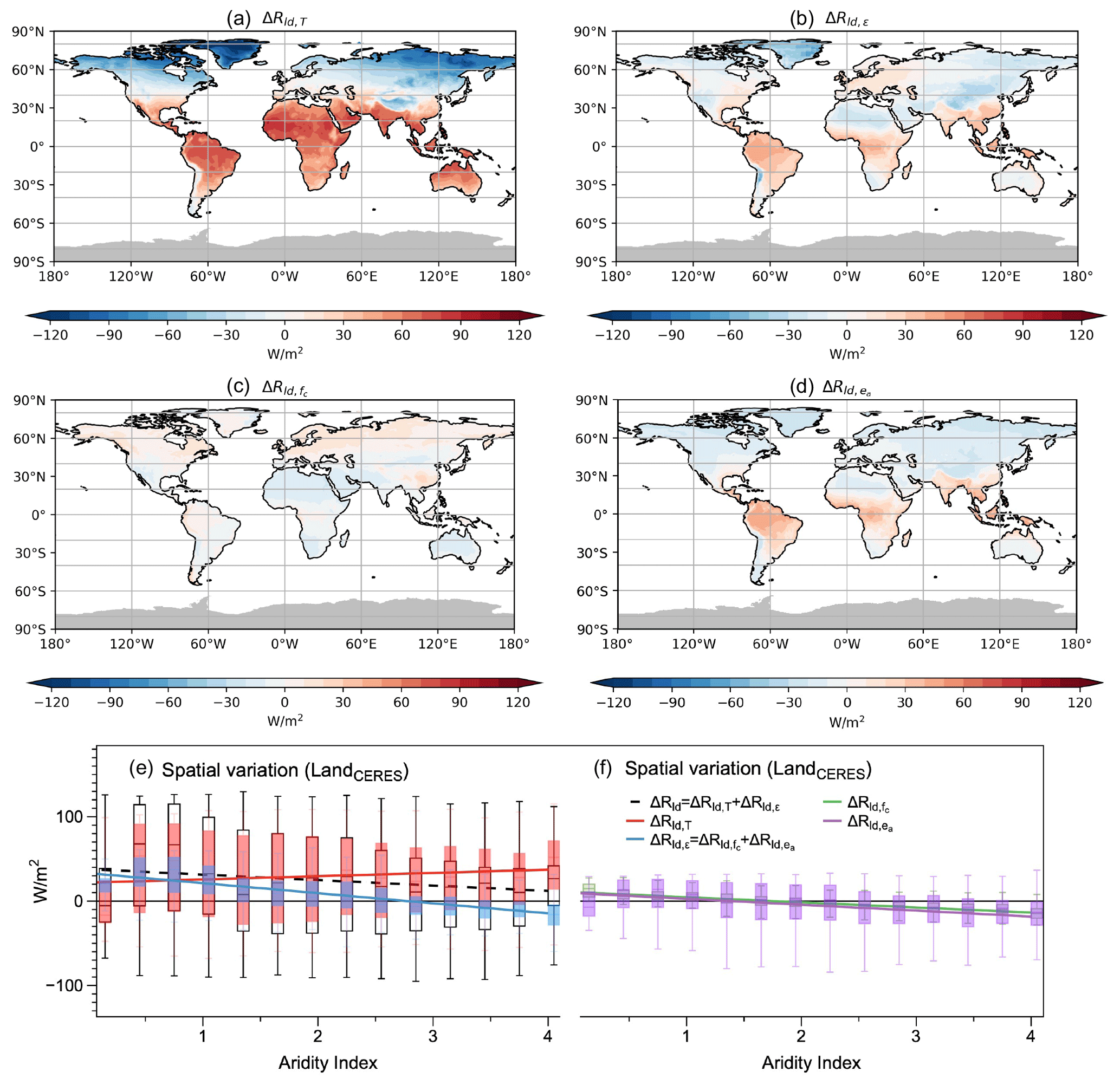
Figure 6 Decompositions of the multi-year-mean spatial variation of R_ld (deviations in the multi-year-mean value for each grid from the land-mean value) in the NASA-CERES dataset into contributions by (a) lower atmospheric heat storage (ΔR_ld,T) and (b) emissivity (ΔR_ld,ε). Decomposition of ΔR_ld,ε into contributions by (c) variations in cloud cover ($\mathrm{\Delta }{R}_{\mathrm{ld},f_{\mathrm{c}}}$) and (d) humidity ($\mathrm{\Delta }{R}_{\mathrm{ld},e_{\mathrm{a}}}$). In (a)–(d), grey shading indicates missing values. In (e) and (f), the box shows the variation among the land grids with the same aridity. The upper and lower whiskers indicate the 95th and 5th percentiles, respectively, and the upper boundary, median line, and lower boundary of the box indicate the 75th, 50th, 25th quantiles, respectively.

These variations are evaluated with respect to the aridity index in Figs. 6e and f and S7. While there is a large spread, as seen in the quantiles, there is a small but consistent trend towards lower values of R_ld in more arid regions, with a magnitude of about −(10–20) W m⁻² across the entire aridity index spectrum (dashed black line in Fig. 6e). We also notice a shift in the contributions, with emissivity contributing less and lower atmospheric heat storage contributing more with increased values of AI. The decreasing contributions in emissivity of about −40 W m⁻² is caused by reductions in cloud cover and water vapor (Fig. 6f), which can be attributed to the common presence of high-pressure systems in subtropical arid areas (Zampieri et al., 2009) and less monsoon there. The decreasing contribution by lower atmospheric emissivity is compensated for by an increased contribution of about +20–30 W m⁻² by atmospheric heat storage that is caused by the generally warmer mean temperatures in arid regions.

4 Discussion and conclusions

We found that the semiempirical equations of Brutsaert (1975) and Crawford and Duchon (1999) work very well to estimate the downwelling flux of longwave radiation by comparing these to estimates from observation, satellite, and reanalysis datasets, with r² ranging from 0.87 to 0.98 across the datasets for clear-sky and all-sky conditions. We then showed that one can use these equations to decompose this flux into different components and relate changes to differences in cloud cover, water vapor, and lower atmospheric heat storage. We found that most diurnal changes in downwelling longwave radiation are caused by differences in lower atmospheric heat storage that are reflected in differences in surface air temperature, with the changes in atmospheric emissivity playing the secondary role. The dominance of surface air temperature can be also observed in the seasonal ranges of R_ld, except in tropical monsoon regions due to large variations in water vapor and cloud cover. As for the spatial variation, from arid to humid regions the increasing lower atmospheric heat storage and decreasing atmospheric emissivity have an offsetting effect on the R_ld variation, thus leading to relatively subtle changes in R_ld along with the aridity index.

Relating our decomposition to radiative kernel helps us gain a more comprehensive understanding of variations in R_ld. Referring to the sensitivity in the downwelling longwave radiation for an incremental change in an atmospheric property (e.g., T_a, f_c, and e_a), the radiative kernel has been used to attribute R_ld changes, based on numerically calculation with radiative transfer code (Previdi, 2010; Zeppetello et al., 2019) or partial differentiating with explicit formula for R_ld (Shakespeare and Roderick, 2022). Following Shakespeare and Roderick (2022), the approximate radiative kernel of T_a, f_c, and e_a are calculated based on Eqs. (8)–(9) (i.e., $\frac{\partial R_{\mathrm{ld}}}{\partial T}=\mathrm{4}\mathit{\sigma }\stackrel{\mathrm{‾}}{\mathit{\epsilon }}{\stackrel{\mathrm{‾}}{T_{\mathrm{a}}}}^{\mathrm{3}}$; $\frac{\partial R_{\mathrm{ld}}}{\partial f_{\mathrm{c}}}=\mathit{\sigma }{\stackrel{\mathrm{‾}}{T_{\mathrm{a}}}}^{\mathrm{4}}\times \left(\mathrm{1}-\stackrel{\mathrm{‾}}{\mathrm{1.24}{\left(\frac{\stackrel{\mathrm{‾}}{e_{\mathrm{a}}}}{\stackrel{\mathrm{‾}}{T_{\mathrm{a}}}}\right)}^{\frac{\mathrm{1}}{\mathrm{7}}}}\right)$; and $\frac{\partial R_{\mathrm{ld}}}{\partial e_{\mathrm{a}}}=\mathit{\sigma }{\stackrel{\mathrm{‾}}{T_{\mathrm{a}}}}^{\mathrm{4}}\times \frac{\mathrm{1.24}}{\mathrm{7}}\frac{\left(\mathrm{1}-\stackrel{\mathrm{‾}}{f_{\mathrm{c}}}\right)}{{\left(\stackrel{\mathrm{‾}}{e_{\mathrm{a}}}\right)}^{\frac{\mathrm{6}}{\mathrm{7}}}{\left(\stackrel{\mathrm{‾}}{T_{\mathrm{a}}}\right)}^{\frac{\mathrm{1}}{\mathrm{7}}}}$) and shown in the left panel of Fig. S8. As shown in Fig S8a, the sensitivity of R_ld to T_a peaks in the tropics with a maximum of around 5 W m⁻² K⁻¹ and decreases at higher latitudes, which is generally consistent with Shakespeare and Roderick (2022). Moreover, the seasonal cycle of the atmospheric properties themselves are shown in the right panel of Fig. S8, which reveals that the spatial distribution of the contribution of T_a, e_a, and f_c to the seasonal variations in R_ld (Fig. 5) is dominated by the seasonal changes of the air properties (Fig. S8b, d, and f) instead of the sensitivity of R_ld to them (Fig. S8a, c, and e).

These equations can then be applied to different aspects of climate research. For instance, the values of downwelling longwave radiation are often missing in FLUXNET data (Table S2), and these equations can be used to fill the gaps with air temperature and humidity observations. We can also use these equations to better understand the physical mechanisms for temperature change due to extreme events. For instance, Park et al. (2015) and Alekseev et al. (2019) found that an enhancement of downwelling longwave radiation in the Arctic is found to be preceded by the advection of moisture and heat. The equations by Brutsaert (1975) and Crawford and Duchon (1999) can then be used to quantify the individual contributions by the advection of heat and moisture (Tian et al., 2022). Another example is the attribution of differences in temperature magnitudes across humid and arid regions (Ghausi et al., 2023). Du et al. (2020) used these equations to explain why global warming was stronger during clear-sky conditions in observations in China due to the greater sensitivity of clear-sky emissivity to a change in water vapor. This was then used to explain the observed, stronger global warming in the arid regions of China, which have fewer clouds and a higher frequency of clear-sky conditions than the humid regions. Furthermore, while the empirical coefficient of 1.24 in Eq. (1) may change due to emissivity changes from greenhouse gases, this formulation can nevertheless provide a useful basis in terms of the interannual changes of R_ld, which is shown in Fig. S9. As shown in Fig. S9a, R_ld increases in most of the land regions at an average rate of 0.64 W m⁻² per decade, with the contribution of increased temperature, increased water vapor, and decreased cloud cover contributing 0.46, 0.28, −0.10 W m⁻² per decade, respectively. Furthermore, it can be observed in Fig. S9d–i that the temperature effect is generally around 0.5 W m⁻² per decade, while the influence of emissivity is significantly dominant in the monsoon region, which is majorly due to the interannual changes in water vapor.

It is worth noting that several effects on R_ld variations are not included in B75 and C&D99, e.g., the well-mixed greenhouse gas concentrations (Shakespeare and Roderick, 2022), large aerosol particles (Zhou and Savijärvi, 2013), and cloud base (Viúdez-Mora et al., 2015). Although rarely influencing the diurnal change, seasonal cycles, and spatial distribution, these terms need attention when the interannual trend of R_ld is investigated under global warming, which can be implied by the difference between Fig. S9a and b. In addition, B75 in conjunction with C&D99 is adopted in this work to decompose the R_ld variations in different spatial–temporal scales, considering its solid physical foundations and the relatively lower computation consumption. Further analysis can be performed based on other estimations, e.g., Prata (1996), which shows consistency with reanalysis data (Allan et al., 2004). The cloud effect can be also detected using the difference between all-sky and clear-sky R_ld (Allan, 2011; Ghausi et al., 2022). Moreover, datasets that are more focused on radiation and energy budget can be used to test the robust of the results, e.g., BSRN (Driemel et al., 2018) and GEBA (Wild et al., 2017).

We conclude that the equations by Brutsaert (1975) and Crawford and Duchon (1999) are still very useful in advancing our understanding of surface temperature changes. Our evaluation has shown how well these equations estimate this flux, and our application to the decomposition of different contributions has shown its utility in understanding the causes of its variation. These equations should help us to better understand aspects of climate variability, extreme events, and global warming, linking these to the mechanistic contributions by downwelling longwave radiation.