The effect of strong nonlinearity on wave-induced vertical mixing

A semi-analytical solution to an advection–diffusion equation is coupled with a nonlinear wavemaker model to investigate the effect of strong nonlinearity on wave-induced mixing. The comparisons with weakly nonlinear model predictions reveal that in the case of waves of higher steepness, enhanced mixing affects the subsurface layer of the water column. A fully nonlinear model captures the neglected higher-order terms from a weakly nonlinear solution and provides a reliable estimation of the time-mean velocity field. The corrected wave-induced mass-transport velocity leads to improved estimates of subsurface mixing intensity and ocean surface temperature.

1 Introduction

Mass-transport processes associated with the propagation of non-breaking ocean surface waves strongly affect the mixing of oceanic waters and the global exchange of heat at the air–water interface. Surface waves transfer energy into turbulence, modifying the mixing intensity of the upper ocean (Qiao et al., 2004, 2010, 2013). Therefore, the correct identification and quantification of mass-transport processes associated with water waves leading to mixing of subsurface ocean waters is of practical importance for short-term and long-term weather forecasts.

Small-scale and large-scale climate modelling equally benefits from including the wave-induced mixing predictions into the general ocean circulation simulations (e.g. Qiao et al., 2004; Xia et al., 2006). Including the parameterized wave-induced mixing in ocean circulation models confirms that its contribution qualitatively improves the reliability of numerical results (e.g. Song et al., 2007; Shu et al., 2011). Despite the fact that some field measurements lead to the conclusion that surface waves contribute to heat exchange of the upper ocean (Matsuno et al., 2006), it is difficult to collect reliable in situ data confirming the role of non-breaking surface waves in vertical mixing processes. An alternative approach to the problem is to investigate the wave-induced mixing based on the physical tests in a wave flume or a wave basin.

Laboratory experiments are the source of valuable information on wave-induced mixing processes as they provide data enabling the evaluation of wave-induced mixing coefficient (e.g. Babanin and Haus, 2009; Dai et al., 2010; Sulisz and Paprota, 2015). In a wave flume, the mixing originated from breaking and non-breaking waves may be investigated to evaluate the real contribution from the non-breaking surface waves to general ocean circulation, which is of fundamental importance for calibration of wave-induced mixing models (Sulisz and Paprota, 2019). It should be noted that the experimental data are affected by undesirable spurious laboratory effects requiring special attention when analysing the results of mass-transport processes driven by waves (e.g. Paprota and Sulisz, 2018; Paprota, 2020).

The study extends the analysis of wave-induced vertical mixing performed by Sulisz and Paprota (2019), which used a weakly nonlinear theory applied to mechanically generated water waves. The improvements cover the more exact calculations of the wave velocity field using a fully nonlinear wavemaker model, which was successfully verified with respect to kinematics of regular waves against laboratory measurements collected in the flume (Paprota and Sulisz, 2018; Paprota, 2020). This method allows modelling of non-breaking waves with strong nonlinearities and admits amplitude dispersion, nonlinear wave–wave interactions in deep and intermediate waters, and solitary wave propagation, which go beyond the applicability of weakly nonlinear approaches. The model belongs to a family of wave solutions based on a pseudo-spectral approach, which consider highly nonlinear non-breaking waves and originate from methods derived by Dommermuth and Yue (1987) and West et al. (1987) (see also Paprota and Sulisz, 2019, for a review).

The application of the fully nonlinear model should lead to the more accurate estimation of the phase-averaged wave velocity field and, hopefully, the more reliable evaluation of the evolving water temperature field under regular waves. Since the numerical model provides a full description of the evolution of the velocity field, it is possible to separate the Stokes drift from Lagrangian and Eulerian mean velocities (see Paprota et al., 2016; Paprota and Sulisz, 2018; Paprota, 2020). Hence, the results presented in this study may improve simple models based on Stokes drift applicable to ocean waves of random (spectral) nature (Myrhaug et al., 2018), while the derived modelling framework may be modified to cover open-ocean hydrodynamics with other forms of introducing waves (Paprota, 2019).

New contributions are also presented with regard to methods of calculations of time-mean flows, which are essential for the present analyses. Namely, a new Eulerian procedure is reported, which is different to the Lagrangian-based method applied in earlier studies (Paprota et al., 2016; Paprota and Sulisz, 2018; Paprota, 2020). The study also highlights the differences between two methods of calculation of velocity distribution of time-mean wave-induced flows based on either Lagrangian particle tracking or approximated Eulerian averaging. In the case of the former, an improved and more accurate procedure of estimating the phase-averaged velocity is developed.

This study presents the methods of an analysis of wave-induced vertical mixing from the wavemaker perspective. The derived mathematical modelling approach may be directly applied to experimental activities aiming at recognizing, quantifying and parameterizing wave-induced vertical mixing effects (see e.g. Dai et al., 2010; Sulisz and Paprota, 2015) for a better design of physical model set-up and a wave parameter selection in the laboratory. The awareness of the influence of laboratory side effects on the experimental outcome is essential for the correct interpretation of the results. This issue was raised in earlier studies (Sulisz and Paprota, 2015, 2019).

The paper is composed as follows. First, an outline of the coupled theoretical model describing the mixing processes under mechanically induced water waves is presented. Then, a comprehensive comparison between weakly and fully nonlinear approaches is given using numerical results to evaluate the effects of strong nonlinearity on vertical mixing processes. Finally, a discussion on the major results is provided together with remarks on accuracy and reliability of mathematical and numerical methods together with further discussions on putting the results of the study in a broader context of earth system modelling with respect to general ocean circulation. The paper is then completed by a summary and conclusions.

2 Materials and methods

The considered numerical approach to the modelling of vertical mixing induced by mechanically generated waves is realized through a procedure involving two fundamental steps referring to the solution of the wavemaker problem and advection–diffusion balance, respectively.

2.1 Particle kinematics of mechanically generated waves

First, the problem of the generation of waves in a numerical wave flume is formulated and solved. In the present study, a potential flow wave theory is used to obtain the solution within the Eulerian frame of reference. Weakly nonlinear analytical and higher-order numerical methods are employed to determine the wave fields in the rectangular domain, in which the water elements are defined by the horizontal x and vertical z coordinates of the Cartesian system. The origin of the system is located at the intersection of the wavemaker zero position and free-surface level corresponding to the hydrostatic conditions. The mechanically driven oscillation of the free surface represented by elevation function η(x,t) is induced by the piston-like motion of the wavemaker paddle according to the displacement function χ(t). The flume bottom is assumed horizontal, and the water depth is h=const. The general presentation of the computational domain and the location of the coordinate system are depicted in Fig. 1.

Figure 1 Schematic view of mechanically generated waves and the coordinate system.

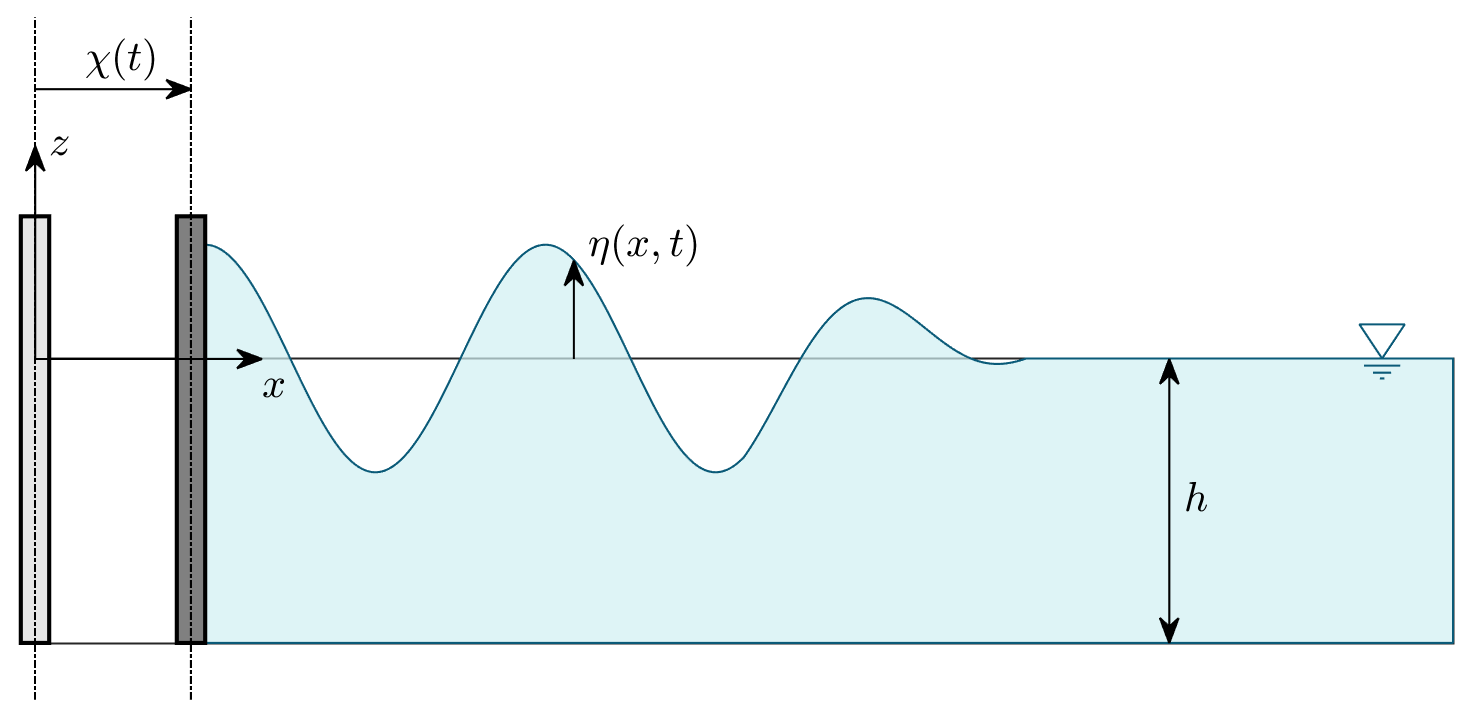
According to the potential flow assumptions, the motion of an inviscid and incompressible fluid is irrotational. Moreover, the solid boundaries are impervious. The scalar velocity potential function $\mathit{\varphi }(x,z,t)$ may be introduced to determine the velocity vector field $\mathit{v}(x,z,t)$ such that v=∇ϕ. The wavemaker boundary-value problem is then formulated as

$$\begin{array}{}\text{(1)}& {\displaystyle }{\mathrm{\nabla }}^{\mathrm{2}}\mathit{\varphi }=\mathrm{0},-h\le z\le \mathit{\eta },\text{(2)}& {\displaystyle }{\mathit{\eta }}_t+{\mathit{\varphi }}_x{\mathit{\eta }}_x-{\mathit{\varphi }}_z=\mathrm{0},z=\mathit{\eta },\text{(3)}& {\displaystyle }{\mathit{\varphi }}_t+{\displaystyle \frac{\mathrm{1}}{\mathrm{2}}}({\mathit{\varphi }}_x^{\mathrm{2}}+{\mathit{\varphi }}_z^{\mathrm{2}})+g\mathit{\eta }=\mathrm{0},z=\mathit{\eta },\text{(4)}& {\displaystyle }{\mathit{\varphi }}_z=\mathrm{0},z=-h,\text{(5)}& {\displaystyle }{\mathit{\chi }}_t-{\mathit{\varphi }}_x=\mathrm{0},x=\mathit{\chi },\end{array}$$

where g is the acceleration due to gravity.

The first part of a pseudo-spectral solution involves expanding the kinematic free-surface boundary condition (2), the dynamic free-surface boundary condition (3) and the kinematic wavemaker boundary condition (5) in a Taylor series about a mean position corresponding to the still water level (z=0) for Eqs. (2)–(3) and wavemaker paddle zero position (x=0) for Eq. (5):

$$\begin{array}{}\text{(6)}& {\displaystyle }\sum _{m=\mathrm{0}}{\displaystyle \frac{{\mathit{\eta }}^m}{m\mathrm{!}}}{\displaystyle \frac{{\partial }^m}{\partial z^m}}({\mathit{\eta }}_t+{\mathit{\varphi }}_x{\mathit{\eta }}_x-{\mathit{\varphi }}_z)=\mathrm{0},z=\mathrm{0},\text{(7)}& {\displaystyle }\sum _{m=\mathrm{0}}{\displaystyle \frac{{\mathit{\eta }}^m}{m\mathrm{!}}}{\displaystyle \frac{{\partial }^m}{\partial z^m}}\left({\mathit{\varphi }}_t+{\displaystyle \frac{\mathrm{1}}{\mathrm{2}}}({\mathit{\varphi }}_x^{\mathrm{2}}+{\mathit{\varphi }}_z^{\mathrm{2}})+g\mathit{\eta }\right)=\mathrm{0},z=\mathrm{0},\text{(8)}& {\displaystyle }\sum _{m=\mathrm{0}}{\displaystyle \frac{{\mathit{\chi }}^m}{m\mathrm{!}}}{\displaystyle \frac{{\partial }^m}{\partial z^m}}({\mathit{\chi }}_t-{\mathit{\varphi }}_x)=\mathrm{0},x=\mathrm{0}.\end{array}$$

In this way, a simple rectangular form of the computational domain is preserved, and the solution procedure is advanced further using either the perturbation or spectral approach. In the present study both weakly nonlinear (perturbation expansions) and fully nonlinear (spectral expansions) solutions are briefly presented and applied to calculate the velocity field for wave-induced mixing calculations. The order of nonlinearity depends on the order of nonlinear terms of Taylor series expansions of boundary conditions. Second-order terms are retained for weakly nonlinear solutions, while the fully nonlinear solution is provided with no upper limit (arbitrary order).

2.1.1 Weakly nonlinear solution

The perturbation expansion is first applied to solve the wavemaker problem defined by Eqs. (1)–(5) according to the solution derived by Hudspeth and Sulisz (1991) and Sulisz and Hudspeth (1993). The monochromatic wavemaker paddle displacement of amplitude s is assumed to be

$$\begin{array}{}\text{(9)}& \mathit{\chi }\left(t\right)=s\sin (\mathit{\sigma }t+\mathit{\phi }),\end{array}$$

which generates periodic waves of the first-order amplitude of a, the angular frequency of σ and the phase φ in the semi-infinite flume domain. Due to the fact that x goes to infinity, the radiation condition (outward propagating waves) is imposed at the far-end lateral boundary of the domain (Hudspeth and Sulisz, 1991).

Using the expansions of the boundary conditions Eqs. (6)–(8) and retaining the terms up to the second order, the weakly nonlinear boundary conditions become

$$\begin{array}{}\text{(10)}& {\displaystyle }{\mathit{\eta }}_t-{\mathit{\varphi }}_z+{\mathit{\varphi }}_x{\mathit{\eta }}_x-\mathit{\eta }{\mathit{\varphi }}_{zz}=\mathrm{0},z=\mathrm{0},\text{(11)}& {\displaystyle }{\mathit{\varphi }}_t+{\displaystyle \frac{\mathrm{1}}{\mathrm{2}}}({\mathit{\varphi }}_x^{\mathrm{2}}+{\mathit{\varphi }}_z^{\mathrm{2}})+\mathit{\eta }{\mathit{\varphi }}_{zt}+g\mathit{\eta }=\mathrm{0},z=\mathrm{0},\text{(12)}& {\displaystyle }{\mathit{\chi }}_t-{\mathit{\varphi }}_x-\mathit{\chi }{\mathit{\varphi }}_{xx}=\mathrm{0},x=\mathrm{0}.\end{array}$$

Additionally, the following small steepness parameter ϵ=ak (where k is the first-harmonic wave number) perturbation expansions of the angular frequency ω (σ=ω₀), the free-surface elevation and the velocity potential functions are used (Hudspeth and Sulisz, 1991):

$$\begin{array}{}\text{(13)}& {\displaystyle }\mathit{\omega }=\sum _{n=\mathrm{0}}{\mathit{ϵ}}^n{\mathit{\omega }}_n,\text{(14)}& {\displaystyle }\mathit{\varphi }(x,z,t)=\sum _{n=\mathrm{0}}{\mathit{ϵ}}^n{\mathit{\varphi }}_{n+\mathrm{1}},\text{(15)}& {\displaystyle }\mathit{\eta }(x,t)=\sum _{n=\mathrm{0}}{\mathit{ϵ}}^n{\mathit{\eta }}_{n+\mathrm{1}}.\end{array}$$

Substituting the perturbation forms Eqs. (13)–(15) into the boundary conditions correct up to the second order, Eqs. (10)–(12), leads to the final weakly nonlinear solution to the velocity potential and free-surface elevation functions (Hudspeth and Sulisz, 1991). The formulas for the horizontal U(x,y) and vertical W(x,y) components of the time-independent mass-transport velocity V(x,y) for the case of the piston-type wavemaker of full-depth draught are calculated from nondimensional forms reported as Eqs. (50a) and (50b) by Hudspeth and Sulisz (1991). In order to get dimensional values, the results calculated by Eqs. (50a) and (50b) in the work of Hudspeth and Sulisz (1991) are multiplied by $a\sqrt{gk}$.

Far away from the wavemaker paddle (x>3h), the vertical component of the time-independent velocity vanishes, and the time-independent horizontal velocity profile along the water depth U_L converges to the sum of the Stokes drift U_S and return current U_E velocities (Longuet-Higgins, 1953; Dean and Dalrymple, 1984), i.e.

$$\begin{array}{}\text{(16)}& U_{\mathrm{L}}\left(z\right)=U_{\mathrm{S}}\left(z\right)+U_{\mathrm{E}},\end{array}$$

where the Stokes drift profile is calculated as

$$\begin{array}{}\text{(17)}& U_{\mathrm{S}}\left(z\right)={\displaystyle \frac{k\mathit{\sigma }{a}^{\mathrm{2}}\cosh \left(\mathrm{2}k\right(z+h\left)\right)}{\mathrm{2}{\sinh }^{\mathrm{2}}\left(kh\right)}},\end{array}$$

and the return current value takes the form

$$\begin{array}{}\text{(18)}& U_{\mathrm{E}}=-{\displaystyle \frac{k\mathit{\sigma }{a}^{\mathrm{2}}\sinh \left(\mathrm{2}kh\right)}{\mathrm{4}kh{\sinh }^{\mathrm{2}}\left(kh\right)}}=-{\displaystyle \frac{a^{\mathrm{2}}kg}{\mathrm{2}\mathit{\sigma }h}}.\end{array}$$

2.1.2 Fully nonlinear solution

An alternative approach, which admits higher-order wave components, is based on the spectral method applied to the wavemaker problem (Paprota and Sulisz, 2018). Contrary to the presented perturbation approach, the waves are generated by an arbitrary function χ(t) in a finite domain of length b, which is sufficiently large to exclude the effect of wave reflection from the far-end wall of the flume. In this regard, only progressive waves are considered to facilitate the comparisons with the weakly nonlinear solution.

The free-surface elevation function is expanded in a Fourier cosine series as

$$\begin{array}{}\text{(19)}& \mathit{\eta }(x,t)=\sum _{i=\mathrm{0}}{a}_i\cos \left({\mathit{\lambda }}_{i}x\right),\end{array}$$

while the corresponding expansion of the velocity potential function is coupled with an additional term satisfying the wavemaker boundary condition (5) to give

$$\begin{array}{}\text{(20)}& \begin{array}{rl}\mathit{\varphi }(x,z,t)& =\sum _{i=\mathrm{0}}{A}_i{\displaystyle \frac{\cosh \left({\mathit{\lambda }}_i\right(z+h\left)\right)}{\cosh \left({\mathit{\lambda }}_{i}h\right)}}\cos \left({\mathit{\lambda }}_{i}x\right)\\ & +B_{\mathrm{0}}\left(\right(x-b{)}^{\mathrm{2}}-(z+h{)}^{\mathrm{2}})\\ & +\sum _{j=\mathrm{1}}{B}_j{\displaystyle \frac{\cosh \left({\mathit{\mu }}_j\right(x-b\left)\right)}{\cosh \left({\mathit{\mu }}_{j}b\right)}}\cos \left({\mathit{\mu }}_j\right(z+h\left)\right),\end{array}\end{array}$$

where ${\mathit{\lambda }}_i=i\mathit{\pi }/b$ and ${\mathit{\mu }}_j=j\mathit{\pi }/h$ are the eigenvalues of the expansions, and the solution coefficients are the functions of time (a_i(t), A_i(t) and B_j(t)). The B_j coefficients are (Paprota and Sulisz, 2018)

$$\begin{array}{}\text{(21)}& B_{\mathrm{0}}={\displaystyle \frac{{\mathit{\chi }}_{t}h+\sum _{m=\mathrm{1}}^M\frac{{\mathit{\chi }}^m}{m\mathrm{!}}\sin \frac{m\mathit{\pi }}{\mathrm{2}}\sum _{i=\mathrm{0}}{\mathit{\lambda }}_i^m{A}_i\tanh \left({\mathit{\lambda }}_{i}h\right)}{\mathrm{2}h(\mathit{\chi }-b)}},\end{array}$$

$$\begin{array}{}\text{(22)}& \begin{array}{rl}{B}_j& ={\displaystyle \frac{\begin{array}{c}-\mathrm{2}\cos \left({\mathit{\mu }}_{j}h\right){\sum }_{m=\mathrm{1}}^M\frac{{\mathit{\chi }}^m}{m\mathrm{!}}\sin \left(\frac{m\mathit{\pi }}{\mathrm{2}}\right)\\ \cdot \sum _{i=\mathrm{0}}\frac{{\mathit{\lambda }}_i^{m+\mathrm{2}}}{{\mathit{\lambda }}_i^{\mathrm{2}}+{\mathit{\mu }}_j^{\mathrm{2}}}{A}_i\tanh \left({\mathit{\lambda }}_{i}h\right)\end{array}}{h\sum _{m=\mathrm{0}}^M{\mathit{\mu }}_j^{m+\mathrm{1}}\frac{{\mathit{\chi }}^m}{m\mathrm{!}}\cos \left(m\mathit{\pi }\right)\tanh ({\mathit{\mu }}_{j}b{)}^{\left|\cos \frac{m\mathit{\pi }}{\mathrm{2}}\right|}}},\\ & j>\mathrm{0}.\end{array}\end{array}$$

The coefficients A_i, B_j and a_i are determined in an iterative solution procedure from the kinematic free-surface boundary condition (6), the dynamic free-surface boundary condition (7) and the kinematic wavemaker boundary condition (8). For a given time t, the unknown coefficients a_i and A_i are calculated using a Fourier transform of η and ϕ as

$$\begin{array}{}\text{(23)}& \begin{array}{rl}& a_i={\displaystyle \frac{\mathrm{2}}{b}}\underset{\mathrm{0}}{\overset{b}{\int }}\mathit{\eta }(x,t)\cos \left({\mathit{\lambda }}_{i}x\right)\mathrm{d}x,\\ & A_i={\displaystyle \frac{\mathrm{2}}{b}}\underset{\mathrm{0}}{\overset{b}{\int }}\mathit{\varphi }(x,\mathrm{0},t)\cos \left({\mathit{\lambda }}_{i}x\right)\mathrm{d}x,\end{array}\end{array}$$

while B_j values are determined using Eqs. (21) and (22). The coefficients are then used to calculate free-surface and velocity potential values using inverse Fourier transforms to advance the solution in time. Hence, time stepping is applied in a physical domain to obtain values of ϕ and η at a new time level. A fourth-order Adams–Bashforth–Moulton predictor–corrector approach is preferred as a time-marching scheme (see e.g. Press et al., 1988), with initial values of $\mathit{\varphi }(x,\mathrm{0},\mathrm{0})=\mathrm{0}$ and $\mathit{\eta }(x,\mathrm{0})=\mathrm{0}$. The wavemaker model used in the present study is reported in the work of Paprota and Sulisz (2018).

The instantaneous wave velocity field is derived by expressing the horizontal u and vertical w velocity components in terms of the spatial derivatives of the velocity potential ϕ_x and ϕ_z, respectively, as

$$\begin{array}{}\text{(24)}& {\displaystyle }\begin{array}{rl}u(x,z,t)& =-\sum _{i=\mathrm{0}}{\mathit{\lambda }}_i{A}_i{\displaystyle \frac{\cosh \left({\mathit{\lambda }}_i\right(z+h\left)\right)}{\cosh \left({\mathit{\lambda }}_{i}h\right)}}\sin \left({\mathit{\lambda }}_{i}x\right)\\ & +\mathrm{2}{B}_{\mathrm{0}}(x-b)\\ & +\sum _{j=\mathrm{1}}{\mathit{\mu }}_j{B}_j{\displaystyle \frac{\sinh \left({\mathit{\mu }}_j\right(x-b\left)\right)}{\cosh \left({\mathit{\mu }}_{j}b\right)}}\cos \left({\mathit{\mu }}_j\right(z+h\left)\right),\end{array}\text{(25)}& {\displaystyle }\begin{array}{rl}w(x,z,t)& =\sum _{i=\mathrm{0}}{\mathit{\lambda }}_i{A}_i{\displaystyle \frac{\sinh \left({\mathit{\lambda }}_i\right(z+h\left)\right)}{\cosh \left({\mathit{\lambda }}_{i}h\right)}}\cos \left({\mathit{\lambda }}_{i}x\right)\\ & -\mathrm{2}{B}_{\mathrm{0}}(z+h)\\ & -\sum _{j=\mathrm{1}}{\mathit{\mu }}_j{B}_j{\displaystyle \frac{\cosh \left({\mathit{\mu }}_j\right(x-b\left)\right)}{\cosh \left({\mathit{\mu }}_{j}b\right)}}\sin \left({\mathit{\mu }}_j\right(z+h\left)\right).\end{array}\end{array}$$

After a fully developed wave motion is achieved, the time-independent wave velocity field may be approximated by time averaging of the instantaneous wave velocity (see Hudspeth and Sulisz, 1991) within the range limited by two in-phase states of regular wave motion (over one wave period, which is either given or calculated from the dispersion relation) as

$$\begin{array}{}\text{(26)}& {\displaystyle }\begin{array}{rl}U(x,z)& =\langle u_x\int u\mathrm{d}t+u_z\int w\mathrm{d}t\\ & +\mathrm{0.5}{u}_{xx}(\int u\mathrm{d}t{)}^{\mathrm{2}}\\ & +\mathrm{0.5}{u}_{zz}(\int w\mathrm{d}t{)}^{\mathrm{2}}\rangle +\langle u\rangle ,\end{array}\text{(27)}& {\displaystyle }\begin{array}{rl}W(x,z)& =\langle w_x\int u\mathrm{d}t+w_z\int w\mathrm{d}t\\ & +\mathrm{0.5}{w}_{xx}(\int u\mathrm{d}t{)}^{\mathrm{2}}\\ & +\mathrm{0.5}{w}_{zz}(\int w\mathrm{d}t{)}^{\mathrm{2}}\rangle +\langle w\rangle \end{array}\end{array}$$

and is referred to here and after as the Eulerian-mean transport velocity (EMTV). The pair of triangle brackets 〈 〉 denotes the operator of time averaging over one wave period. The velocities u and w are calculated using Eqs. (24) and (25), while their derivatives are evaluated analytically. The integrals of u and w are determined directly from Eqs. (24) and (25) upon replacing the time-dependent coefficients A_i and B_j with their integrals ∫A_idt and ∫B_jdt. The integration is achieved by expanding A_i and B_j into a Fourier series with respect to time and integrating the resulting Fourier expansions analytically.

An alternative approach, which leads to the time-independent wave velocity field, is the procedure involving the Lagrangian particle tracking: Lagrangian-mean transport velocity (LMTV). The time-averaged velocity is calculated based on the displacement of a water particle moving between its two successive in-phase positions along the particle trajectory (Paprota et al., 2016). The trajectory of a water particle is determined by numerical integration of the system of differential equations,

$$\begin{array}{}\text{(28)}& {\displaystyle \frac{\mathrm{d}x}{\mathrm{d}t}}=u(x,z,t),\text{(29)}& {\displaystyle \frac{\mathrm{d}z}{\mathrm{d}t}}=w(x,z,t),\end{array}$$

for the set of initial particle locations.

In the present study, the improvements to the method of evaluation of mass-transport velocity based on the Lagrangian particle tracking (Paprota and Sulisz, 2018) are introduced. In the previous works (Paprota et al., 2016; Paprota and Sulisz, 2018; Paprota, 2020), the procedure relied on distributing artificial tracers in a water column under fully developed regular waves. Initially, the tracers are uniformly distributed along the water depth, and they coincide with the zero down-crossing phase of the wave for a given distance from the wavemaker. After one Lagrangian wave period (see e.g. Longuet-Higgins, 1986; Chen et al., 2009), the tracers move from their original position due to mass transport. The particle tracking procedure is employed to determine the mass-transport velocity profile. The procedure is repeated for subsequent longitudinal positions to cover the accepted region of interest.

Here, in order to get the better estimation of the time-independent velocity field, the two hydrodynamic states corresponding to both zero up- and down-crossings of the regular wave are used to start up the tracking procedure – contrary to the previous method based only on the zero down-crossings (e.g. Paprota et al., 2016; Paprota and Sulisz, 2018). The procedure is analogous but involves more tracers and covers two phase positions. The resulting LMTV is calculated as the mean of the time-independent velocity fields corresponding to both zero-crossing initial states.

2.2 Wave-induced vertical mixing intensity

The numerical solution to a two-dimensional advection–diffusion equation with relevant boundary conditions is used to predict the evolution of the temperature field under mechanically generated regular waves in the flume. Assuming that the changes in temperature are solely due to wave-induced and diffusion processes, the following boundary-value problem is formulated as in the work of Sulisz and Paprota (2019):

$$\begin{array}{}\text{(30)}& {\displaystyle }{T}_t+U{T}_x+W{T}_z={\partial }_x\left(\mathit{\kappa }{T}_x\right)+{\partial }_z\left(\mathit{\kappa }{T}_z\right),\text{(31)}& {\displaystyle }{T}_z=\mathrm{0},z=\mathrm{0},\text{(32)}& {\displaystyle }{T}_x=\mathrm{0},x=\mathrm{0},\text{(33)}& {\displaystyle }{T}_z=\mathrm{0},z=-h,\text{(34)}& {\displaystyle }{T}_x=\mathrm{0},x=b,\end{array}$$

where T is the water temperature, and κ is the diffusion coefficient represented as a sum of the molecular (κ_m) and wave-induced (κ_v) diffusivities.

$$\begin{array}{}\text{(35)}& \mathit{\kappa }={\mathit{\kappa }}_{\mathrm{m}}+{\mathit{\kappa }}_{\mathrm{v}}\end{array}$$

In the advection–diffusion equation (30) the velocities U an W are, in fact, Lagrangian velocities which describe the mean transport velocity field (the Stokes drift and a return current in this case). The inclusion of the Stokes drift (without return current) to the advection equation was discussed explicitly for the case of ocean waves by McWilliams and Sullivan (2000).

The molecular diffusivity ${\mathit{\kappa }}_{\mathrm{m}}=\mathrm{1.4}\times {\mathrm{10}}^{-\mathrm{7}}$ m s⁻², while the wave-induced diffusivity is calculated by the formula reported by Sulisz and Paprota (2015) as

$$\begin{array}{}\text{(36)}& {\mathit{\kappa }}_{\mathrm{v}}\left(z\right)=\mathit{\alpha }{a}^{\mathrm{3}}k\mathit{\sigma }{\displaystyle \frac{{\sinh }^{\mathrm{2}}\left(k\right(z+h\left)\right)\cosh \left(k\right(z+h\left)\right)}{{\sinh }^{\mathrm{3}}\left(kh\right)}},\end{array}$$

where α=0.002 is the dimensionless coefficient, which is evaluated based on measurements (Sulisz and Paprota, 2015). The derivation of κ_v is based on the weakly nonlinear theory. More information is provided in the work of Sulisz and Paprota (2015), where the comparison between the weakly nonlinear and more general forms is provided. The parameter α was estimated based on the experiments only for the presented form of κ_v. In order to use a more general formula, new values of α must be determined using experimental data from a wider range of wave conditions.

The advection–diffusion equation (Eq. 30) holds in the entire fluid domain, while the heat radiation is assumed zero at the water surface (Eq. 31), the bottom (Eq. 33) and the lateral boundaries (Eqs. 32 and 34). The length b is sufficiently long in order to reduce the effect of the finite domain on the results in the area of interest, which is limited to the region of several water depths from the wavemaker paddle. The omitted procedure of incorporating the non-zero heat radiation at the water surface is discussed in the paper by Sulisz and Paprota (2019).

The solution of the advection–diffusion equation (Eq. 30) is achieved by employing a similar methodology to that used to solve the wavemaker problem admitting higher-order nonlinearities presented in the previous section. Accordingly, the scalar temperature field function is expanded into a double Fourier series of the form (Sulisz and Paprota, 2019)

$$\begin{array}{}\text{(37)}& T(x,z,t)=\sum _{i=\mathrm{1}}\sum _{j=\mathrm{1}}{d}_{ij}\cos \left({\mathit{\lambda }}_i\right(x-b\left)\right)\cos \left({\mathit{\mu }}_j\right(z+h\left)\right).\end{array}$$

Again, the solution of Eq. (30) is achieved by a time-stepping procedure, which, in this case, consists of an application of the spectral expansion method to describe T and the Runge–Kutta formulas to proceed in time (see e.g. Press et al., 1988). Accordingly, the wave-induced diffusivity is determined using Eq. (36), while the velocity field is calculated by means of either the weakly nonlinear solution (Hudspeth and Sulisz, 1991) or a higher-order approach (Paprota and Sulisz, 2018) for selected wave parameters. The initial condition of given vertical temperature distribution T₀(z) is used to start up the time-stepping procedure. The time derivative of temperature T is calculated from Eq. (30) with the aid of the expansion Eq. (37) after the coefficients d_ij are determined by applying a two-dimensional cosine fast Fourier transform. The implementation of this procedure is freely available in Paprota (2023).

3 Results and discussion

The evaluation of temperature evolution of an oscillating water body is analysed in a numerical wave flume environment. This approach provides a basis for the straightforward verification of the major outcome of the modelling procedures, which are presented in the previous section, against measurements in the real laboratory. On the other hand, the numerical model may be modified to cover pseudo-random ocean waves in a large periodic domain (see e.g. Paprota, 2019) to analyse the wave-induced vertical mixing processes in offshore conditions.

3.1 Numerical test cases

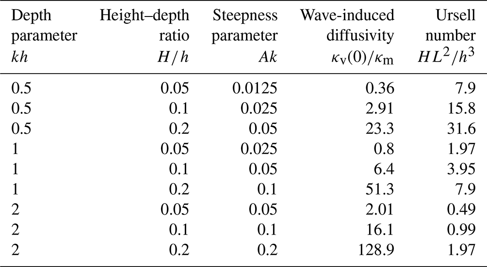
The waves are generated by a monochromatic wavemaker motion in a numerical flume. The transitional and shallow water wave cases are considered for three values of the depth-relative dimensionless parameter kh of 0.5, 1 and 2. The effect of wave height H is also studied and corresponds to the dimensionless steepness parameter $H/h$ of 0.05, 0.1 and 0.2. In the case of the higher-order solution, the waves are generated starting from rest with the ramp function applied to the stroke of the wavemaker motion for the first five wave periods. As previously stated, the longitudinal size of the flume b is sufficiently large to exclude wave reflections from the analysis, and it corresponds to 10 wavelengths (L) for kh=2 and 20L in the remaining longer wave cases. The selected progressive wave parameters are the same as in previous studies on the modelling of wave-induced mixing in wave flumes (Sulisz and Paprota, 2019). After the fully developed state is achieved, the time-independent wave velocity field is determined. The resulting horizontal and vertical velocity components U and W are then substituted in Eq. (30), and the temperature field evolution is predicted. A summary of wave parameters is provided in Table 1 together with wave-induced diffusivity values at the surface in relation to its molecular counterpart.

Table 1 Basic dimensionless parameters of mechanically generated regular waves.

It should be noted that the model may be applied to deep-water as well as shallow-water conditions, which are presented in the work of Sulisz and Paprota (2015). Here, the cases correspond to a limited range of kh from 0.5 to 2.0. In this way, the results from the previous work (Sulisz and Paprota, 2019) may be directly compared. Moreover, for deep-water conditions corresponding to kh>π, the mixing would completely sweep away the warmer water from the analysed part of the fluid domain for the selected time frame, and this case was omitted in the present study.

3.2 Phase-averaged velocity distribution

The accurate assessment of the time-independent velocity field is of significant importance in the modelling of temperature changes under an undulating water surface. The increasing steepness of generated waves intensifies wave-induced mixing processes but also changes the structure of heat flux distribution in the region occupied by the fluid. The analysis of phase-averaged velocity distribution in the direct vicinity of the wavemaker paddle helps to identify the effect of advection terms of Eq. (30) on the temperature evolution driven by waves.

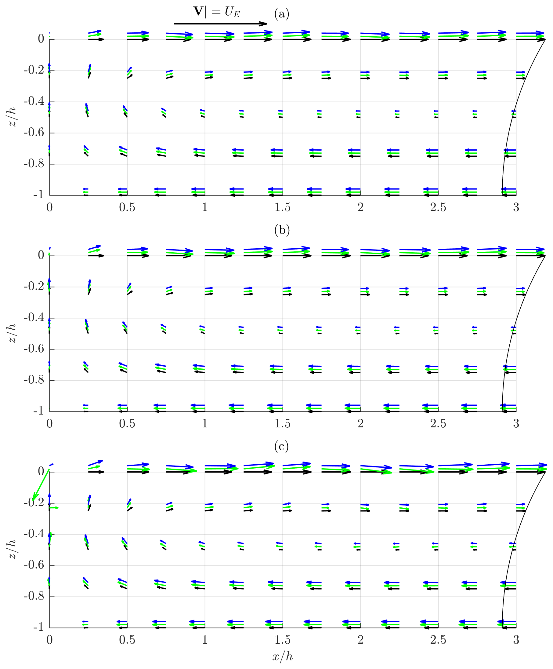
Figure 2 Time-independent velocity field under mechanically generated regular waves characterized by kh=0.5, (a) $H/h=\mathrm{0.05}$, (b) $H/h=\mathrm{0.1}$ and (c) $H/h=\mathrm{0.2}$. Weakly nonlinear theory – black arrows and line, higher-order-theory EMTV – green arrows, LMTV – blue arrows. Higher-order vectors are shifted upwards for convenience of comparison.

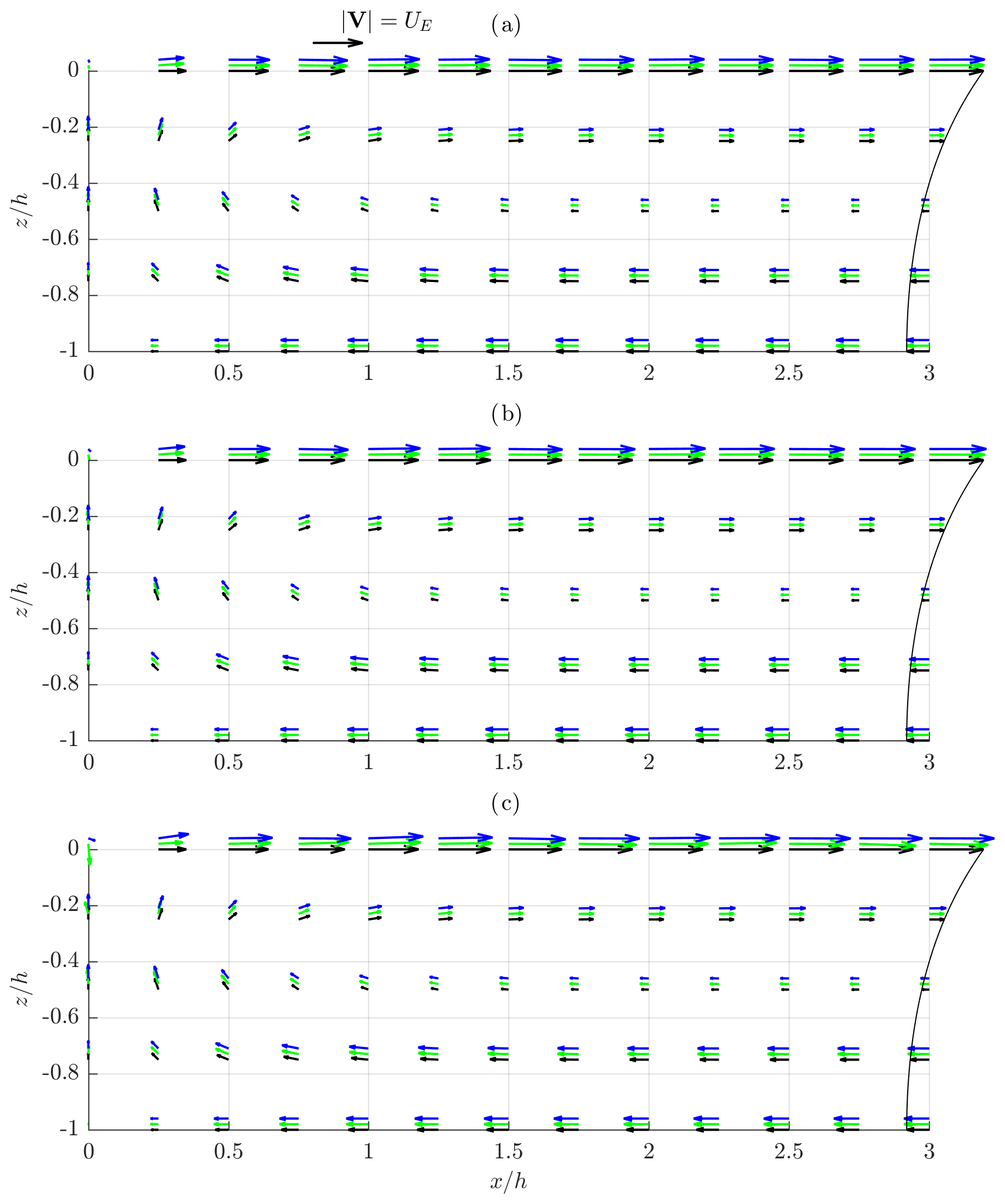
Figure 3 Time-independent velocity field under mechanically generated regular waves characterized by kh=1, (a) $H/h=\mathrm{0.05}$, (b) $H/h=\mathrm{0.1}$ and (c) $H/h=\mathrm{0.2}$. Weakly nonlinear theory – black arrows and line, higher-order-theory EMTV – green arrows, LMTV – blue arrows. Higher-order vectors are shifted upwards for convenience of comparison.

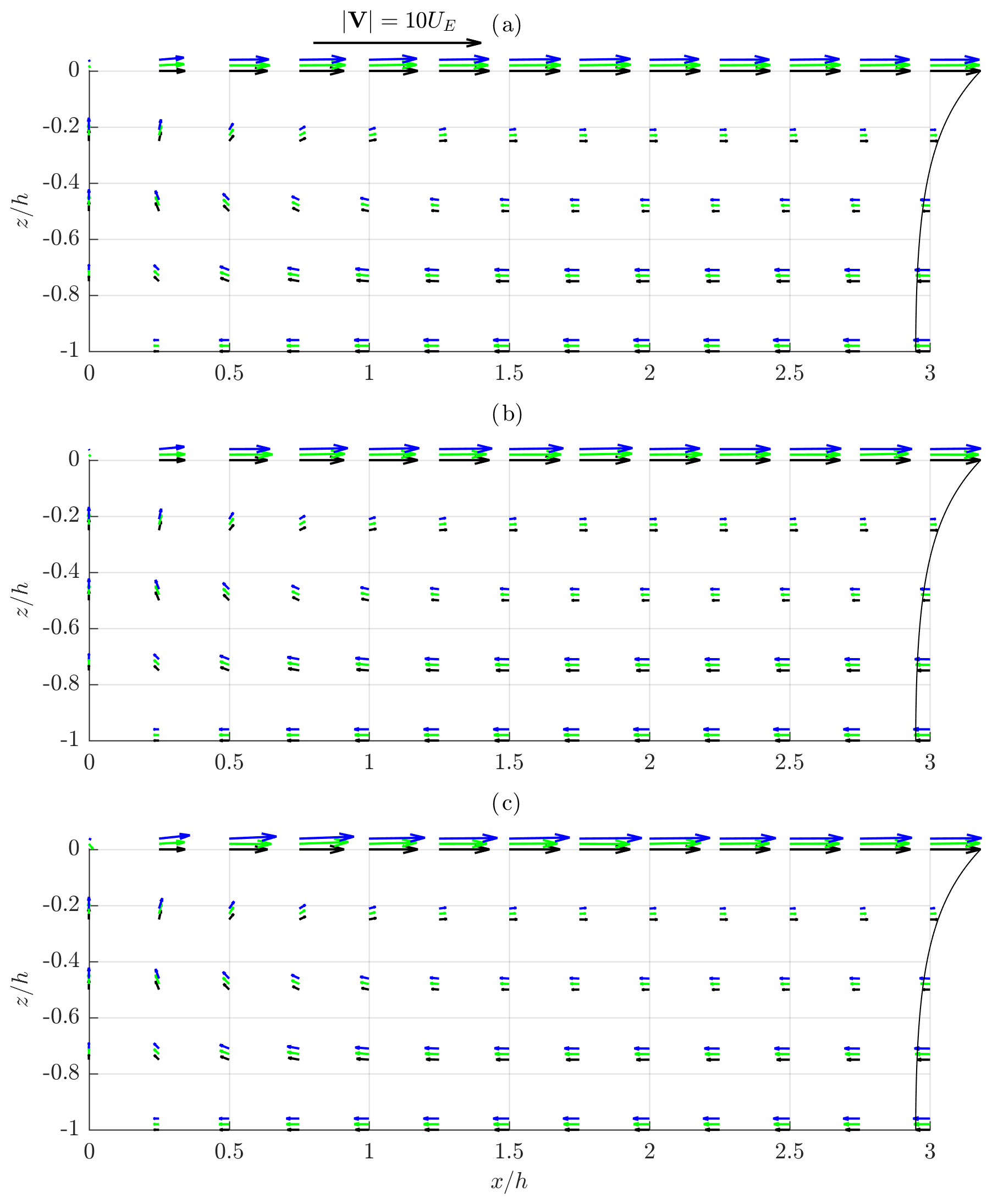
Figure 4 Time-independent velocity field under mechanically generated regular waves characterized by kh=2, (a) $H/h=\mathrm{0.05}$, (b) $H/h=\mathrm{0.1}$ and (c) $H/h=\mathrm{0.2}$. Weakly nonlinear theory – black arrows and line, higher-order-theory EMTV – green arrows, LMTV – blue arrows. Higher-order vectors are shifted upwards for convenience of comparison.

In Figs. 2–4, time-independent velocity fields calculated by weakly nonlinear and higher-order methods are presented. The arrows represent the vectors of a phase-averaged velocity corresponding to mass transport induced by waves. Black arrows correspond to a weakly nonlinear solution, while green and blue arrows correspond to a higher-order solution and two methods of averaging – EMTV and LMTV, respectively (Figs. 2–4). The way the results are presented is in line with the expected velocity vector field pattern in the part of the fluid domain adjacent to the wavemaker (see Paprota and Sulisz, 2018, for a more detailed description). The fluid flow forms half of the circulation cell limited by the air–water interface ($z/h=\mathrm{0}$), the wavemaker paddle ($x/h=\mathrm{0}$) and the bottom ($z/h=-\mathrm{1}$). The water mass flows with the direction of wave propagation near the surface, while the adverse flow pushes the water to the wavemaker paddle in the lower part of the water column. At the wavemaker paddle, the water flows vertically, forming the lateral boundary of the general circulation in the flume. Far away from the paddle, the vertical velocity components vanish, and the typical mass-transport velocity profile over depth emerges as a sum of the Stokes drift Eq. (17) and the return current velocity Eq. (18). Thus, the figures are complemented by the weakly nonlinear horizontal mass-transport velocity profile U_L(z) calculated outside the direct vicinity of the wavemaker paddle Eq. (16), where the effect of evanescent standing waves generated by the wavemaker (see e.g. Dean and Dalrymple, 1984) may be neglected (x>3h). U_L(z) is plotted at the right outer edge of the graph at x=3h for convenience of comparison. Vector plots are complemented by bubble charts of relative differences between corresponding vector magnitudes as presented in Figs. 5–7, where black circles denote the differences between LMTV and weakly nonlinear results, while filled green circles refer to the differences between LMTV and EMTV.

Figure 5 Relative differences for time-independent velocity field under mechanically generated regular waves characterized by kh=0.5, (a) $H/h=\mathrm{0.05}$, (b) $H/h=\mathrm{0.1}$ and (c) $H/h=\mathrm{0.2}$. LMTV vs. weakly nonlinear theory – black circles, LMTV vs. EMTV – filled green circles.

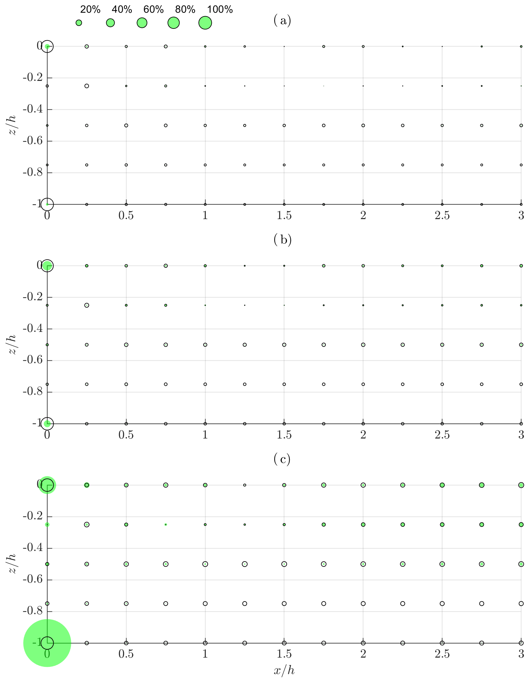
Figure 6 Relative differences for time-independent velocity field under mechanically generated regular waves characterized by kh=1, (a) $H/h=\mathrm{0.05}$, (b) $H/h=\mathrm{0.1}$ and (c) $H/h=\mathrm{0.2}$. LMTV vs. weakly nonlinear theory – black circles, LMTV vs. EMTV – filled green circles.

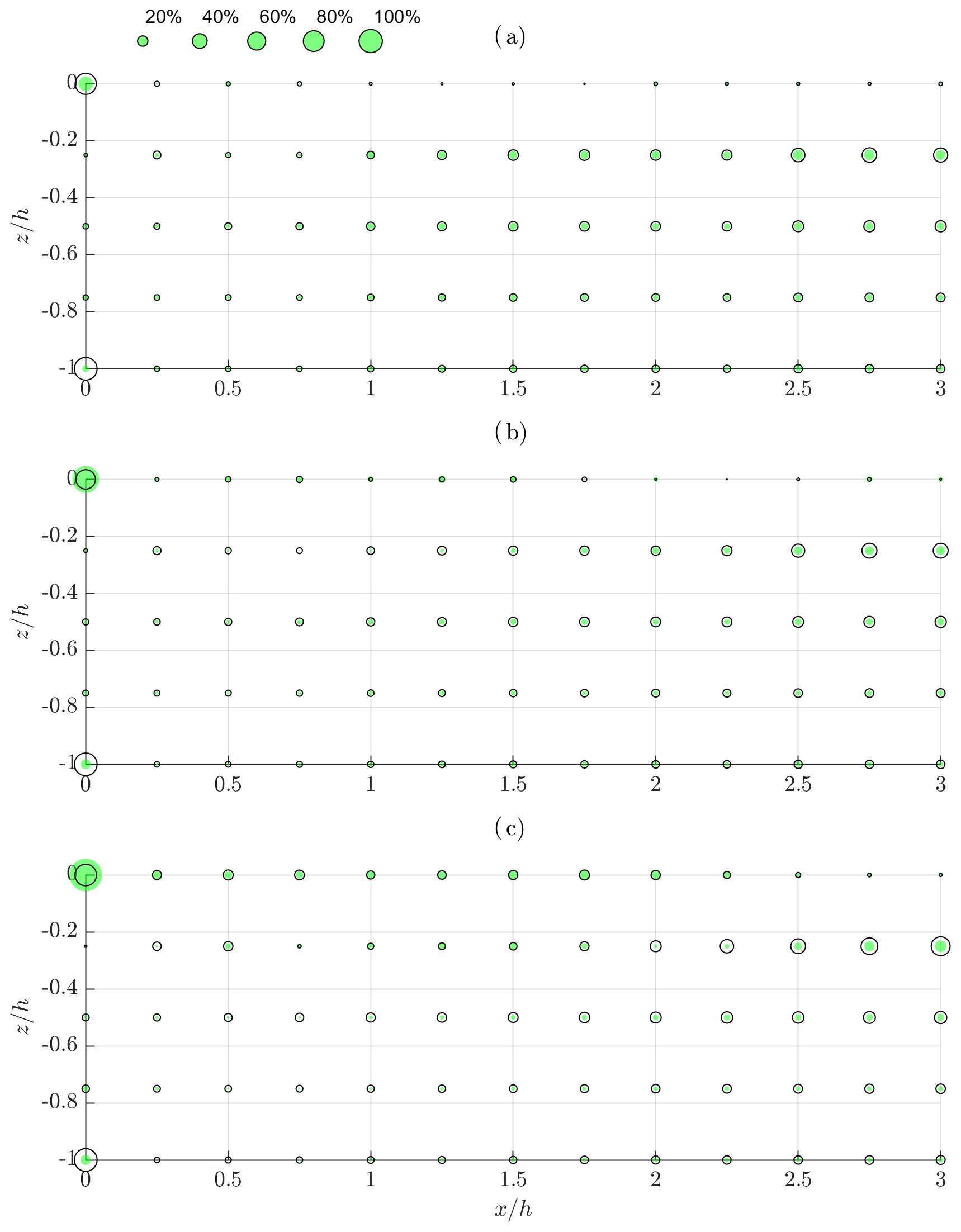
Figure 7 Relative differences for time-independent velocity field under mechanically generated regular waves characterized by kh=2, (a) $H/h=\mathrm{0.05}$, (b) $H/h=\mathrm{0.1}$ and (c) $H/h=\mathrm{0.2}$. LMTV vs. weakly nonlinear theory – black circles, LMTV vs. EMTV – filled green circles.

The results presented in Fig. 2 provide information on the time-independent velocity field predicted in the direct vicinity of the wavemaker paddle and the differences between the weakly nonlinear approach and the solution admitting higher-order terms in the most extreme nonlinear regime of shallow water (kh=0.5). Due to the fact that the considered wave cases are characterized by the highest values of the Ursell number, the differences between the two wavemaker models immediately appear even for the lowest amplitude of free-surface oscillations of $H/h=\mathrm{0.05}$ (Fig. 2a). The highest differences in the range between 10 % and 20 % correspond to the velocities near the wavemaker paddle and the surface, respectively (Fig. 5a). By increasing the magnitude of the surface oscillations to $H/h=\mathrm{0.1}$ and $H/h=\mathrm{0.2}$ (Fig. 2b and c), the differences become higher in the larger area of the wavemaker paddle vicinity. The higher-order model predicts more intensive mass transport near the bottom and the surface. The increase in the subsurface velocity and the magnitude of the current near the bottom may even reach from 15 % to 30 % for $H/h=\mathrm{0.1}$ and from 20 % to 40 % for $H/h=\mathrm{0.2}$ (Fig. 5b and c, respectively).

Some important information may also be acquired from the comparison between two methods of averaging corresponding to either Lagrangian particle tracking (LMTV) or Eulerian averaging (EMTV) based on Eqs. (26) and (27), respectively. Although both methods of averaging provide consistent results for lower wave heights of the generated waves, EMTV results are less reliable in the case of the highest waves $H/h=\mathrm{0.2}$ (Fig. 2c). It can be seen that the velocity vectors near the corner point determined by the intersection of the wavemaker paddle mean position and the surface ($x/h=\mathrm{0}$, $z/h=\mathrm{0}$) are unnaturally large as the velocity in this area (green arrows around the point (0,0) in Figs. 2c and 3c) is expected to vanish (see Grilli and Svendsen, 1990, for a comprehensive discussion on numerical methods' inaccuracy at corner points of a fluid domain with moving boundaries). The problem still persists when considering the subsurface velocity at some distance away from the wavemaker. The differences between the LMTV and EMTV may even reach 20 % in the velocity magnitude near the intersection between the wavemaker and the surface, while an even greater discrepancy is visible at corner points in most extreme longer-wave cases (Fig. 5c).

With increasing relative water depth (Figs. 3 and 4), the differences between weakly nonlinear and higher-order time-independent velocity are less pronounced but still significant for steeper waves. In the case characterized by kh=1, the discrepancies are generally less then 10 % for $H/h=\mathrm{0.05}$ and 0.1, ranging from 10 % to 20 % for the highest waves (Fig. 6). Again the more intensive mass circulation is apparent when higher-order terms are taken into account for the case of kh=1 and $H/h=\mathrm{0.2}$ (Fig. 3c). Similar conclusions may be drawn for the deeper water kh=2 (Fig. 4). However, in the case of the mass-transport velocity profile relatively far away from the wavemaker paddle (x=3h) the differences are twice as high as in the wave cases corresponding to kh=1. It should be noted that, for higher kh (Fig. 7), the results corresponding to two methods of averaging are more consistent; however the highest difference may still reach 20 % as in the case of longer waves (Fig. 5c).

Putting aside the problems with averaging of the velocity field, the general conclusion from the analysis of the results depicted in Figs. 2–7 is that admitting higher-order terms of the Taylor series expansions of the boundary conditions imposed at the moving boundaries leads to more accurate prediction of the time-independent velocity near the wavemaker as expected. This is of significant importance especially for the modelling of wave-induced mixing and the evolution of the water temperature field as the higher-order approach predicts enhanced streaming in layers adjacent to the bottom and the surface. This leads to more intense mixing processes and heat exchange.

3.3 Evolution of a temperature field

The modelling of wave-induced vertical mixing in terms of the temperature redistribution in the water column relies on the solution to the two-dimensional boundary-value problem defined by Eqs. (30)–(34). The input parameters being introduced to the governing advection–diffusion equation (Eq. 30) are the diffusion coefficient κ_v calculated using Eqs. (35) and (36) and the time-independent wave velocity field (U, W). The modelling procedure remains in accordance with previously published results (Sulisz and Paprota, 2019) with different velocity field input. The temperature T₀(z) determines the initial thermal state of the fluid (Fig. 8).

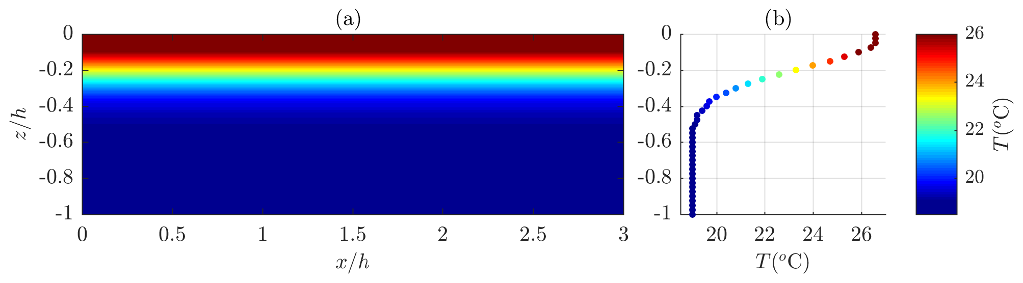
Figure 8 Initial temperature in the fluid domain. (a) Spatial distribution, (b) vertical profile.

In Figs. 9–11, the temperature spatial distributions representing the thermal states of the undulating water body after 100 s is provided for the test cases listed in Table 1. The results in the plots correspond to a weakly nonlinear solution and higher-order model predictions of the time-independent wave velocity field. Both methods are compared in order to highlight the effects of nonlinearity on vertical mixing due to waves.

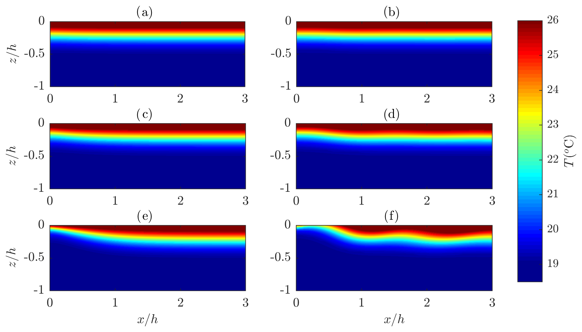
Figure 9 Changes in the temperature field due to waves after 100 s for kh=0.5, (a, b) $H/h=\mathrm{0.05}$, (c, d) $H/h=\mathrm{0.1}$ and (e, f) $H/h=\mathrm{0.2}$. Weakly nonlinear theory (a, c, e; left), higher-order theory (b, d, f; right).

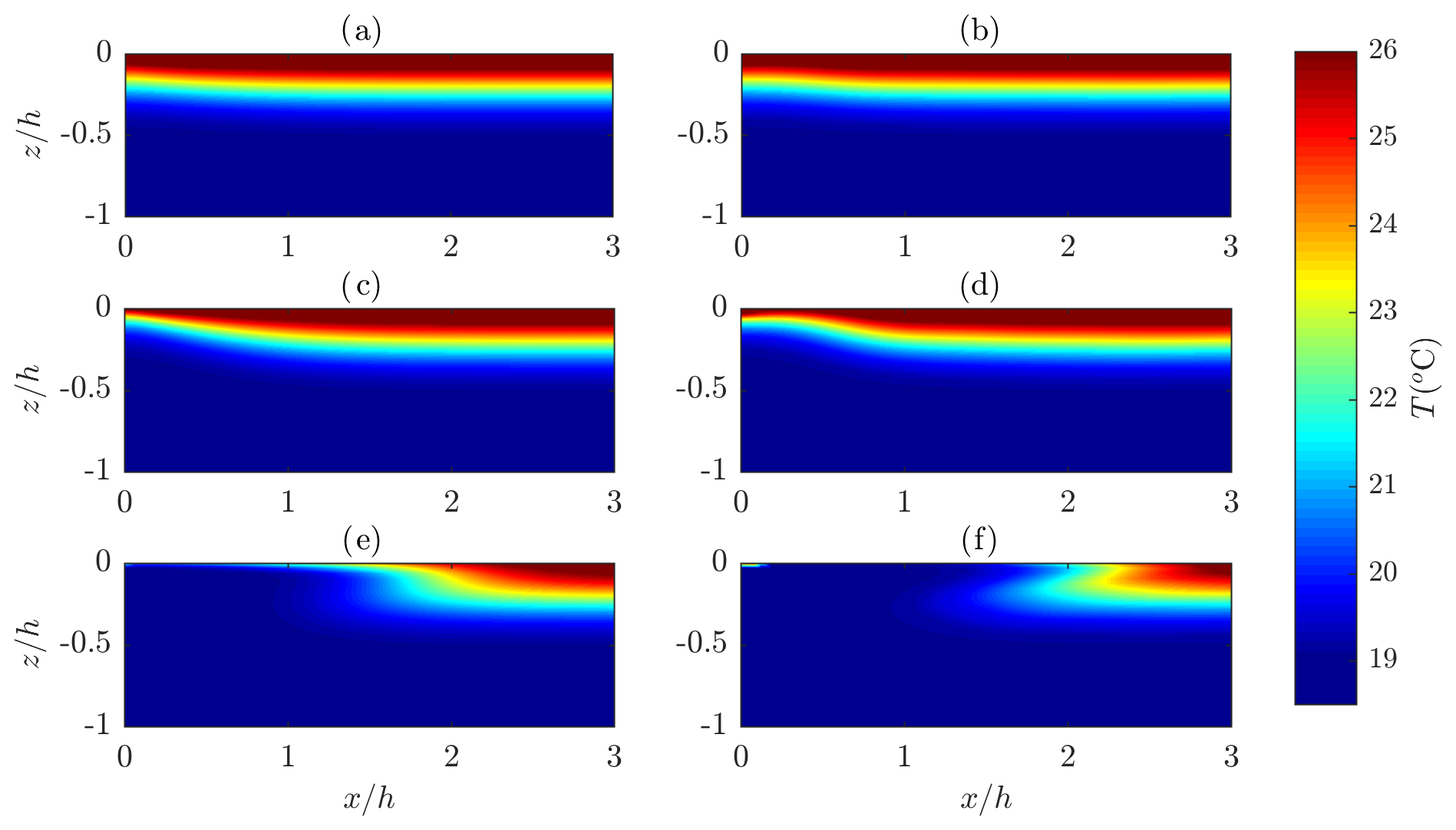
Figure 10 Changes in the temperature field due to waves after 100 s for kh=1, (a, b) $H/h=\mathrm{0.05}$, (c, d) $H/h=\mathrm{0.1}$ and (e, f) $H/h=\mathrm{0.2}$. Weakly nonlinear theory (a, c, e; left), higher-order theory (b, d, f; right).

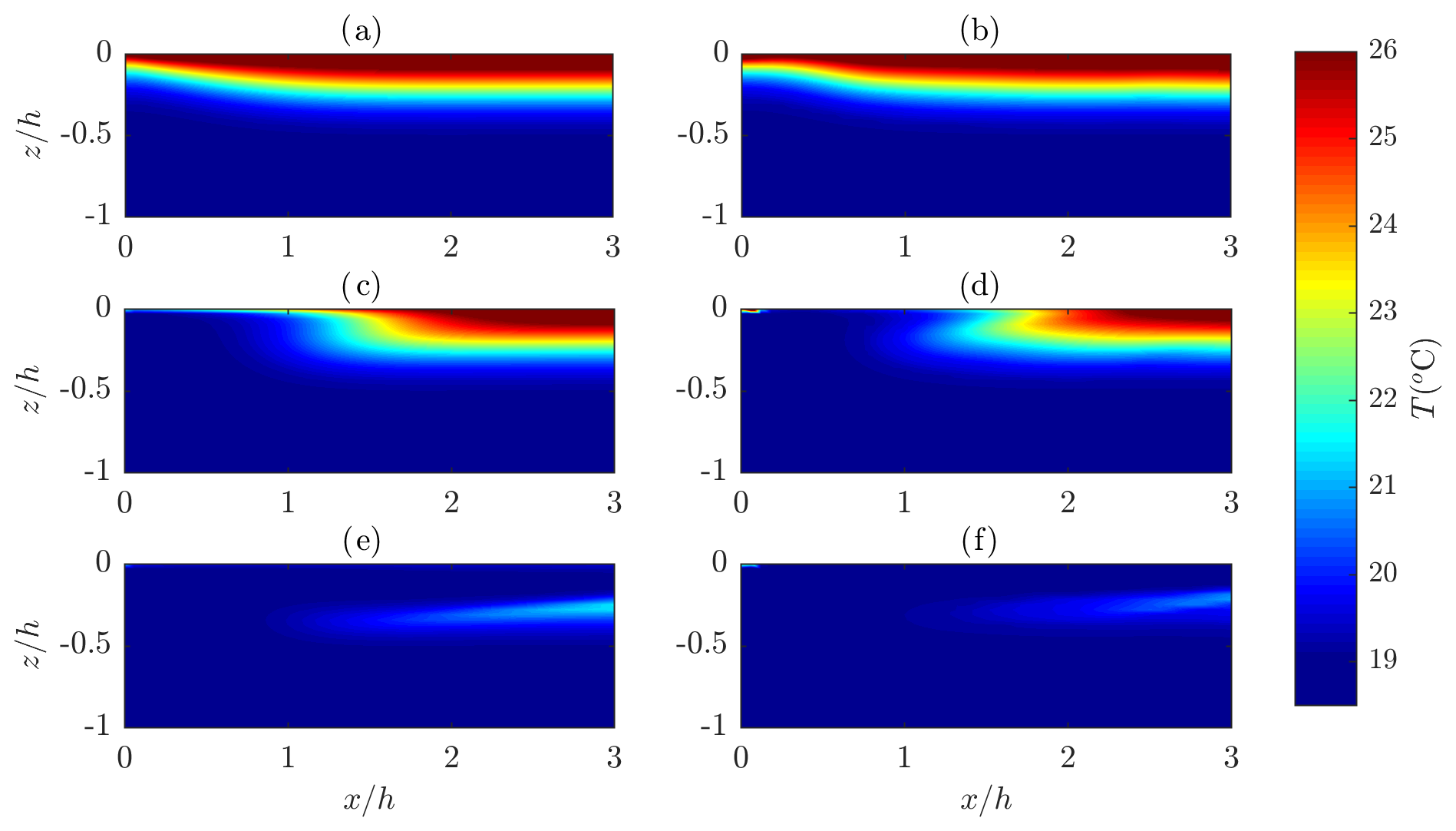
Figure 11 Changes in the temperature field due to waves after 100 s for kh=2, (a, b) $H/h=\mathrm{0.05}$, (c, d) $H/h=\mathrm{0.1}$ and (e, f) $H/h=\mathrm{0.2}$. Weakly nonlinear theory (a, c, e; left), higher-order theory (b, d, f; right).

In the direct vicinity of the wavemaker paddle, the initial state of the water temperature is uniformly stratified according to T₀. The moving wavemaker paddle generates regular waves, and the layers of water of equal temperature are deformed by the oscillatory motion of the water body according to the time-independent velocity field presented in Figs. 2–4. Advection plays an important role in wave-induced mixing processes as even small changes in the velocity strongly affect the evolution of the temperature field. This implies major differences between weakly nonlinear and higher-order predictions of the resultant temperature when the steepness of waves increases. This effect is clearly seen in Figs. 9–11. As previously stated, the discrepancy between weakly nonlinear velocities and the velocity predictions admitting higher-order terms in the free-surface boundary conditions grows with increasing steepness and wave nonlinearity (Ursell number) and may even reach 40 % in the subsurface layer.

Although the highest relative differences are relevant for the longest waves, the effect of including higher-order terms is most apparent for waves of the largest kh characterized by the highest time-independent velocities. It may be seen in Fig. 9 that after 100 s the colder water is moved to the surface close to the wavemaker only for the steepest waves (Fig. 9f) when predicted by the higher-order model, while for the corresponding weakly nonlinear temperature field this process is less intensive (Fig. 9e). Additionally, the higher-order results exhibit some variation in mixing along the flume (Fig. 9f).

In the case of waves characterized by kh=1, the wave-induced mixing is more intensive (see Table 1), and for the steepest waves (Fig. 10e, f) the warmer water is moved away from the wavemaker. It should be noted that the higher-order solution predicts enhanced streaming near the surface (Fig. 10f). In this way, the decreased water surface temperature affects regions located further away from the wavemaker when compared to weakly nonlinear results (Fig. 10). The similar temperature field modification affects the waves of kh=2, but for the lower analysed height (cf. Figs. 10e, f and 11c, d). In the case of the highest waves of kh=2, the warmer water is almost completely swept away from the region of direct wavemaker action (Fig. 11e, f).

3.4 Further discussions

Energy input from wind to ocean surface waves is tremendous and exceeds 60 TW (Wang and Huang, 2004). A large amount of energy dissipates, which implies stirring and mixing processes in the oceanic mixed layer. A parameterization scheme for surface wave-induced mixing was proposed, and numerical experiments indicate that this parameterization affects the performance and outcome of ocean circulation models (Qiao et al., 2004, 2010; Xia et al., 2006) as well as climate predictions (Song et al., 2007; Huang et al., 2008). Although field observations suggest that surface waves can generate vertical mixing (Matsuno et al., 2006), it is still difficult to distinguish the mixing originating from the variety of processes that accompanied ocean waves. Although the problem of wave-induced vertical mixing is of significant importance for physical oceanographers and climatologists, the research on this subject is still in its infancy. Wave-induced mixing is a very important process from a practical point of view and is a challenging problem for theoretical investigations. The understanding of wave-induced mixing is of fundamental importance for the modelling and accurate prediction of ocean transport processes and climate changes. The problem is that the parameterization scheme applied in the modelling and prediction of ocean surface wave-induced mixing is based on drastic simplifications. Wave models derived using simplifying assumptions cannot be applied to predict ocean surface wave-induced mixing with sufficient accuracy. The present studies clearly show that it is necessary to apply at least a weakly nonlinear wave theory to obtain reasonable results (no wave-induced mass transport in linear theory means no heat exchange along the direction of wave propagation), while an increased accuracy is possible using advanced nonlinear wave models admitting higher-order effects. It should also be noted that in the present studies the effects of turbulence and the development of viscous boundary layers are neglected, while these processes may have some impact on larger timescales. For example, the mass-transport velocity profile changes due to the effects of viscosity near the boundaries (the undulating free surface and the bottom) for a sufficiently long time interval, which was studied theoretically by Longuet-Higgins (1953) and also investigated experimentally in a wave flume (see e.g. Swan, 1990; Grue and Kolaas, 2017).

There is one more critical outcome from the point of view of engineers and scientists working on the modelling of ocean transport processes, wave-induced mixing and climate changes. Namely, since it is difficult to distinguish the mixing that accompanied ocean waves, the only chance to provide reliable insight into the wave-induced mixing processes is to conduct laboratory experiments in a wave flume. The repeatable experiments in the well-controlled environment of a wave flume enable us to perform an accurate investigation that is essential in the analysis of the physics of the wave-induced mixing phenomenon. Moreover, laboratory investigations provide useful data for the analysis of the correlations between spectral and statistical characteristics of wave regimes and wave-induced mixing processes. Finally, laboratory experiments enable us to avoid various side effects and separate the mixing from other processes that accompanied ocean waves such as wave breaking. This is of fundamental importance for understanding of mixing and accurate calibration and verification of numerical models. The problem is that, in addition to progressive laboratory waves, the moving wavemaker represented by the kinematic wavemaker boundary condition enforces the return current that affects transport processes and wave-induced mixing.

It is the idea behind the present study, which employs a numerical wave flume model, to thoroughly analyse wave-induced mixing effects using the derived numerical approach and assist further works on experimental fluid mechanics aiming at better understanding of transport processes in the open ocean. To the best of the authors' knowledge, the derived wave-induced mixing approach is the only available numerical solution that, in addition to nonlinear free-surface boundary conditions, also satisfies the kinematic wavemaker boundary condition. Accordingly, the wavemaker model admits a return current and may be applied to quantify and separate the effects of the return flow on wave-induced mixing processes. The presented results should hopefully improve simple models based on the Stokes drift applicable to random ocean waves (Myrhaug et al., 2018). As previously mentioned, the derived modelling framework may be modified to cover open-ocean conditions for the periodic domains and quasi-random sea states using other forms of wave excitation (Paprota, 2019).

4 Conclusions

The applicability of the wave-induced mixing model for waves generated in a wave flume is validated based on the solution admitting higher-order nonlinearities. In the range of wave conditions covering transitional and shallow waters, the weakly nonlinear results are in reasonable agreement with the more accurate pseudo-spectral solution in the case of waves of low to moderate steepness. The general discrepancy grows by increasing the wave height and the wavelength. Unlike the weakly nonlinear approach, the higher-order model is able to predict enhanced subsurface streaming affecting the evolution of the surface temperature for more severe sea states. It is due to the fact that the time-independent velocity field predicted by both methods differs especially in the subsurface and near-bottom layers of the oscillating water body.

General ocean circulation models admitting wave-induced vertical mixing but relying on simplified assumptions cannot predict input from mixing with sufficient accuracy. It is necessary to apply at least a weakly nonlinear correction to obtain reasonable approximation. For improved predictions, advanced highly nonlinear models are preferred, which is confirmed by the present study. Moreover, the derived method allows a return current to be correctly quantified in experimental investigations on wave-induced vertical mixing for better interpretation of laboratory results, giving more information for further improvements to parametrization schemes.