the Creative Commons Attribution 4.0 License.
the Creative Commons Attribution 4.0 License.
 | 25 Oct 2023
A quantitative assessment of air–sea heat flux trends from ERA5 since 1950 in the North Atlantic basin
Johannes Mayer
Leopold Haimberger
Michael Mayer
This work aims to investigate the temporal stability and reliability of trends in air–sea heat fluxes from ERA5 forecasts over the North Atlantic basin for the period 1950–2019. Driving forces of the trends are investigated using analyzed state quantities from ERA5. Estimating trends from reanalysis data can be challenging as changes in the observing system may introduce temporal inconsistencies. To this end, the impact of analysis increments is discussed. For individual sub-regions in the North Atlantic basin, parametrization formulas for latent and sensible heat fluxes are linearized to quantitatively attribute trends to long-term changes in wind speed, moisture, and temperature. Our results suggest good temporal stability and reliability of air–sea heat fluxes from ERA5 forecasts on sub-basin scales and below. Regional averages show that trends are largely driven by changes in the skin temperature and atmospheric advection (e.g., of warmer or drier air masses). The influence of modes of climate variability, such as the North Atlantic Oscillation (NAO) and Atlantic Multidecadal Oscillation, on the patterns found is discussed as well. Results indicate a significant impact on trends in the Irminger and Labrador seas associated with more positive NAO phases during the past 4 decades. Finally, we use basin-wide trends of air–sea heat fluxes in combination with an observational ocean heat content estimate to provide an energy-budget-based trend estimate of the Atlantic Meridional Overturning Circulation (AMOC). A decrease in area-averaged air–sea heat fluxes in the North Atlantic basin suggests a decline in the AMOC over the study period. However, basin-wide flux trends are deemed partially artificial, as indicated by temporally varying moisture increments. Thus, the exact magnitude of change is uncertain, but its sign appears robust and adds complementary evidence that the AMOC has weakened over the past 70 years.
- Article
(11606 KB) - Full-text XML
- BibTeX
- EndNote


The North Atlantic Ocean plays a central role for weather and climate in Europe and eastern North America. For instance, the formation of tropical cyclones and severe weather systems along the Gulf Stream and its extension have a significant impact on our economy, agriculture, and society. The North Atlantic Oscillation (NAO; Hurrell, 1995; Visbeck et al., 2001), a periodic change in strength of the Azores High and Icelandic Low, impacts the moisture transport in the Northern Hemisphere on seasonal timescales and thus influences temperature and precipitation in wide areas of Europe and North America. In addition, the Gulf Stream current in the western North Atlantic is responsible for the poleward transport of oceanic energy that is taken up in tropical latitudes and released to the atmosphere further north via air–sea fluxes. The associated cooling of the waters is required to trigger deep water formation, which is the main driver of the Atlantic Meridional Overturning Circulation (AMOC; Rahmstorf et al., 2015) and consequently also of the global thermohaline circulation. Previous research used climate models to demonstrate that the AMOC has declined over past decades as a result of anthropogenic global warming, which could have further effects on storms and weather patterns (Fox-Kemper et al., 2021). However, direct observations of the AMOC are limited in time and do not show clear evidence of an externally forced slowdown (Baehr et al., 2007; Roberts et al., 2014; Worthington et al., 2021).
In all these processes, the exchange of energy (and momentum) between the atmosphere and underlying ocean is of vital importance. Long-term changes in air–sea heat fluxes over the North Atlantic Ocean can thus have a wide range of implications. Consequently, it is of high relevance to accurately estimate air–sea heat flux trends, which also helps to understand numerous aspects of climate variability in the North Atlantic basin. Nonetheless, observation-based estimates are spatially limited and are available only for the past 2 to 3 decades (see, e.g., ocean site flux data provided by the NOAA; https://www.pmel.noaa.gov/gtmba/, last access: 27 August 2023), making the distinction between anthropogenic changes and natural variability on decadal to multidecadal timescales demanding. For instance, the Atlantic Multidecadal Oscillation (AMO; Kerr, 2000) describes a natural variability mode of basin-wide sea surface temperature (SST) anomalies on timescales of 70–80 years so that its long-term effect on air–sea heat fluxes cannot be determined adequately from observations.
An alternative to observations is given by recent reanalysis data such as the fifth-generation global reanalysis data produced by the ECMWF (ERA5; Hersbach et al., 2020) providing global gridded data for more than 7 decades thanks to its recent preliminary back extension (Bell et al., 2021). Reanalysis data are constructed from past model forecasts constrained by observational data (such as in situ, satellite, airplane, or radiosonde data) through data assimilation, which warrants optimal combination and reduction in biases. However, changes in the observing system can result in temporal discontinuities and introduce increments between forecasts and analyses that may alter the atmospheric state (moisture, temperature, and wind; see Chiodo and Haimberger, 2010 and Mayer et al., 2021) and consequently also air–sea heat fluxes, making climate trend studies with reanalysis data challenging.
Reanalysis data can also be used to indirectly estimate net air–sea heat fluxes (FS) by evaluating the atmospheric energy budget (Trenberth, 1991; Mayer et al., 2016; Trenberth and Fasullo, 2017; Liu et al., 2017; Mayer et al., 2019, 2021, 2022; Liu et al., 2022). This method does not inherently reduce temporal discontinuities but allows the application of a global wind field correction (Trenberth, 1991; Fasullo and Trenberth, 2008; Mayer and Haimberger, 2012), which diminishes both artificial noise over high topography and temporal discontinuities introduced by changes in the observing system (Mayer et al., 2021). Although air–sea heat fluxes derived from ERA5 in this way are available only for the period from 1985 onward (due to the limited availability of observationally constrained top-of-the-atmosphere (TOA) fluxes; see Liu et al., 2020 and Mayer et al., 2022), they are proven to be temporally relatively stable over the global ocean (around 1.7 W m−2 mean based on 1985–2018) and thus can serve as a reference to test the reliability of other commonly used air–sea heat flux products (Mayer et al., 2021, 2022).
This work aims to investigate the reliability and temporal stability of long-term trends of winter-month (December–February) net air–sea heat fluxes based on ERA5 data over the North Atlantic ocean during 1950–2019. Main drivers of trends in latent and sensible heat fluxes are identified based on analyzed state quantities, and the impact of the assimilation process and climate variability modes, such as the NAO and AMO, is discussed. Whenever possible, net air–sea heat fluxes from ERA5 are compared with indirect estimates from Mayer et al. (2022). In four individual sub-regions, turbulent air–sea heat flux trends are quantitatively attributed to long-term changes in wind speed, moisture, and temperature using linearized flux parameterization formulae. Finally, we use basin-wide net air–sea heat fluxes from ERA5 forecasts and an observation-based ocean product to indirectly estimate trends of the AMOC over the past 70 years and discuss sources of uncertainties and reliability of the trend estimate.
The data we use in this study are introduced in Sect. 2. Section 3 describes the methodology. Results are presented in Sect. 4 and summarized and discussed in Sect. 5.
The data we primarily use in this study are from the ECMWF's most recent reanalysis ERA5 (Hersbach et al., 2020). ERA5 provides hourly estimates of a variety of meteorological variables as analyzed state quantities as well as 12-hourly twice-daily forecasts on a Gaussian grid equivalent to 0.25∘ spatial resolution (see Hersbach et al., 2020 for details; Hersbach et al., 2023). Individual components of the net air–sea heat flux (i.e., shortwave and longwave radiation and sensible and latent heat flux) are taken as monthly means and are available only as forecasts. These net air–sea heat fluxes from ERA5 forecasts are denoted as model-based FS hereafter. We also employ temperature and moisture in the lowest model level as well as surface pressure, 10 m wind, near-surface atmospheric density, and skin temperature fields as monthly means from both analyses and forecasts to compute turbulent air–sea heat fluxes using parameterizations as implemented in the Integrated Forecast System (IFS; see ECMWF, 2021), which allows an estimation of the role of changes in single input variables (moisture, temperature, and wind speed; trends in air density are in general not discussed as they are negligibly small). The 3D horizontal wind fields used to compute the meridional mass stream function are also taken from ERA5 but on pressure levels and a regular 0.25 × 0.25∘ grid.
Whenever possible, we compare model-based heat fluxes with indirectly estimated net air–sea heat fluxes (denoted as inferred FS) from Mayer et al. (2022), which are derived from the DEEP-C TOA flux product (see Liu et al., 2020) and atmospheric energy transports from Mayer et al. (2022b) (see also Mayer et al., 2021, and Sect. 2 in Mayer et al., 2022, for details of the computation and assessment). Inferred heat fluxes are provided as monthly averages on a 1∘ regular grid covering 1985–2020.
Observationally constrained ocean heat content (OHC) data are provided by the Institute of Atmospheric Physics (IAP; Cheng et al., 2017; available at http://www.ocean.iap.ac.cn/pages/dataService/dataService.html, last access: 27 August 2023) on a regular 1 × 1∘ grid covering the whole study period from 1950–2019. We use the 0–300 m OHC monthly data for the correlation and comparison with the skin temperature from ERA5 and the 0–2000 m OHC to indirectly estimate the AMOC trend from the oceanic heat budget. The IAP dataset is constructed based on a modified version of the ensemble optimal interpolation method proposed by Cheng and Zhu (2016). Sampling errors are minimized using observational data and a prior guess from Coupled Model Intercomparison Project Phase 5 (CMIP5) multimodel simulations. The small sampling error indicates a robust reconstruction of the temperature signal in all ocean basins. Furthermore, the dataset is bias-corrected using in situ observations (from expendable and mechanical bathythermographs) and thus appears to be well suited for our evaluations.
In addition, we use mooring-derived and volume-conserving monthly ocean heat transport (OHT) estimates from Tsubouchi et al. (2018) and Tsubouchi et al. (2020) as the northern choke point of the oceanic heat budget. Tsubouchi et al. (2018) offer transport estimates from the Davis Strait (DS; see http://metadata.nmdc.no/metadata-api/landingpage/0a2ae0e42ef7af767a920811e83784b1, last access: 27 August 2023) covering the period 1993–2016. Tsubouchi et al. (2020) provide observations for 2005–2010 from the Fram Strait and Barents Sea opening (FS and BSO; see https://doi.org/10.1594/PANGAEA.909966).
3.1 Bulk formulas
In this study, sensible and latent heat fluxes are taken from 12-hourly ERA5 forecasts. However, (i) to estimate the impact of analysis increments on long-term flux trends and (ii) for regression on input variables, we compute fluxes from scratch as described in the following.
Net air–sea heat fluxes (FS) are the sum of radiative and turbulent heat fluxes. Radiative fluxes contain short- and longwave radiation and are not discussed in detail here. Turbulent heat fluxes are the sum of latent and sensible heat fluxes and can be approximated by the commonly used bulk formulas (see Fairall et al., 2003; Cronin et al., 2019; ECMWF, 2021), which are written as follows:
where CQ and CH are non-constant transfer coefficients (see also ECMWF, 2021), ρ is the air density above ocean, Lv (2.5008 × 10⁶ J kg−1) is the latent heat of vaporization, cp (1004.709 ) is the specific heat capacity of dry air, g (9.80665 m s−2) is the gravitational acceleration, and zml is the height of the lowest model level. |Uml|, qml, and Tml are the wind speed, specific humidity, and air temperature at the lowest model level; qsfc is the surface saturation humidity, and Tskin is the skin temperature (as used in the IFS instead of the sea surface temperature); qsfc depends on surface pressure psfc and Tskin and can be derived from the Clausius–Clapeyron relation for 100 % relative humidity. Input variables at the lowest model level and above the ocean are with good approximation 10 m above the surface. According to Eqs. (1) and (2), fluxes from the atmosphere into the ocean are positive.
Whenever fluxes are computed with the above formulae, transfer coefficients are indirectly approximated for each grid point by dividing latent and sensible heat fluxes from ERA5 forecasts with the other terms of the right hand side of Eqs. (1) and (2) (also from forecasts), which has to be done before flux anomalies are computed. This procedure works remarkably well for the ice-free ocean. Over sea ice, however, differences between model-level and surface quantities can be very small (i.e., mean climatology of absolute temperature and moisture differences can be ≤ 0.01 K and ≤ 0.01 g kg−1) so that the division by small numbers introduces artificial noise.
Seasonal trends are computed from monthly anomalies by subtracting the climatology of each grid point and subsequently averaging over December–February. The statistical significance of seasonal trends is computed with the 95 % confidence level and consideration of lag-1 autocorrelation. Analysis increments of model-level variables (temperature and humidity) are calculated at 06:00 and 18:00 UTC from the difference between analyzed state quantities and 12 h forecasts valid at those times. During data assimilation, changes in the observing system can introduce analysis increments that may add or remove temperature or humidity from the model, resulting in unrealistic trends (Bengtsson et al., 2004; Trenberth et al., 2011; Hersbach et al., 2020; Mayer et al., 2021). Uncertainties in model-based FS trends caused by analysis increments are thus estimated by taking the difference between fluxes computed with analyzed state quantities and with short-term forecasts of those quantities.
In this study, we closely follow the mathematical interpretation of air–sea heat fluxes (i.e., Eqs. 1 and 2) and assume that the derived flux trends are solely caused by changes in their input variables (air density, wind, moisture, and temperature). We are aware that this is not the physically correct interpretation as changes in fluxes also influence the input variables due to their mutual dependency (e.g., an increase in latent heat flux increases the moisture in the lowest model level, which in turn reduces latent heat fluxes). However, we argue that in equilibrium (i.e., considering long-term changes over multiple decades) this mutual influence is irrelevant for such discussions so that long-term flux trends can be considered to be a direct result of trends in input variables.
3.2 Linearization of turbulent heat fluxes and partial trends
To attribute trends in latent and sensible heat fluxes to trends in their input variables in a more quantitative way, we linearize the bulk formulas by decomposing each input variable x (ρ, U, q, and T) into their mean state and deviation from its mean x′ (known as Reynolds decomposition; see also Tanimoto et al., 2003, and Yang et al., 2016); that is, each input variable on the right side of Eqs. (1) and (2) is described by . After some calculus, computed turbulent heat fluxes can be further separated into a non-linear and linear part (see Appendix A). The latter contains all products with at most one deviation term on which input variables are regressed to obtain a linear relation between trend in air–sea heat flux F (sensible or latent heat) and trend of each input variable, which reads as follows:
where ξ is a placeholder for either q or T. We term the expressions on the right partial trends, which are the product of the mean sensitivity (i.e., regression of F on x using the whole period of time) and linear trend of input variable x. The mean sensitivity describes how F changes when x is changed. Consequently, partial trends on the right side tell us how much of the flux trend () is explained by the trend in one of the input variables (). Note that this procedure neglects trends in transfer coefficients and the non-linear part, which is a sufficient assumption for the purpose of this study as their contribution to the total turbulent heat flux trend is rather small (the linear part explains ≥ 93 % of the total turbulent flux trend). Furthermore, we do not show partial trends of ρ in our evaluations as they are negligibly small.
3.3 Study area and box averages
Our general study area includes the ice-free ocean between 0–90∘ N and 90∘ W–30∘ E, but particular focus is laid on four 8×8∘ boxes for which partial trends of latent and sensible heat fluxes are computed. The four focus regions are located in the Norwegian Sea (NWS; 68–76∘ N, 2–10∘ E), over the northern flank of the North Atlantic warming hole (NAWH; 55–63∘ N, 37–29∘ W), along the Gulf Stream extension (GS; 35–43∘ N, 66–58∘ W), and in the tropical North Atlantic (TNA; 15–23∘ N, 40–32∘ W) as trends in these regions are associated with distinct atmospheric and oceanic thermodynamics (see Fig. 1). Spatially averaging over these areas reduces the variance of fluxes and computational cost, while trends are still captured reasonably well.
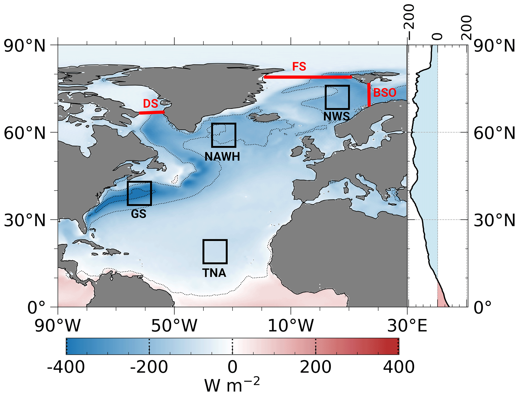
Figure 1Mean 1985–2019 December–February climatology of model-based FS. Black boxes indicate the four areas of interest located in the Norwegian Sea (NWS), North Atlantic warming hole (NAWH), Gulf Stream (GS), and tropical North Atlantic (TNA). The red lines mark the mooring locations in the Davis Strait (DS), Fram Strait (FS), and Barents Sea opening (BSO), which are used to indirectly estimate the ocean heat transport in the North Atlantic basin. Contour lines are shown for 0, ± 200 and ± 400 W m−2.
3.4 Meridional mass stream function
The seasonal mean meridional mass stream function Ψm is obtained by
where rE is the Earth's radius, and is the seasonal mean of the deviation of the meridional wind component (on pressure levels) from its meridional mean, which is vertically integrated from the TOA to the pressure level of interest (p) and over all longitudes λ.
3.5 Indirect estimation of oceanic heat transports
We indirectly estimate the vertically integrated oceanic heat transport at a specific latitude of interest φ in the North Atlantic basin using the oceanic heat budget equation in the following form:
where OHT is the heat transport through the choke point φC (from DS + FS + BSO mooring-derived estimates; see red lines in Fig. 1), and the second term on the right side is the difference between net air–sea heat flux (FS; from ERA5 forecasts) and temporal ocean heat content tendency (OHCT; from 0–2000 m IAP data) integrated over the ocean area between φC and φ (the Mediterranean Sea is excluded; units are watts). This is the same approach as used by Trenberth and Fasullo (2017), Mayer et al. (2022), and Baker et al. (2022) to indirectly estimate heat transports through the RAPID (Johns et al., 2011; McCarthy et al., 2015; Bryden et al., 2020; see also Fig. 1 in Mayer et al., 2022) and SAMBA arrays, respectively. OHTφ is calculated for every fifth latitude between 0–60∘ N (φC is situated between 67–80∘ N). Additionally, we adjust net heat fluxes by subtracting the monthly difference between global ocean mean vertically integrated 0–2000 m OHCT and FS (denoted as R) uniformly from each grid point of the global ocean, as done, for example, by Trenberth et al. (2019). This removes inconsistencies between air–sea heat fluxes and OHCT and guarantees temporal consistency in a global manner (see also Trenberth et al., 2019; Liu et al., 2020; Mayer et al., 2022).
To indirectly estimate the AMOC trend over the whole study period, we extend the 2005–2010 OHT climatology of the choke point DS + FS + BSO to 1950–2019 under the assumption that the upward OHT trend at high latitudes is relatively weak (Muilwijk et al., 2018; Wang et al., 2019, 2020; Docquier and Koenigk, 2021) compared to trends at low latitudes and basin-wide heat flux trends. Trends of indirectly estimated OHT are computed in two ways, with monthly data and 5-year means, using the procedure described by Loeb et al. (2022) (see Sect. 3.2 therein) to estimate trend uncertainties; that is, the effective sample size takes into account all significant autocorrelation functions γ up to lag m where and is satisfied. If these conditions are not satisfied for the autocorrelation at any lag, the true instead of the effective sample size is used to estimate uncertainties.
3.6 Computation of climate indices
The AMO index is calculated similarly to the approach suggested by Trenberth and Shea (2006), where global-mean SST anomalies are subtracted from the spatially averaged SST time series of the North Atlantic basin (0–60∘ N and 0–80∘ W). The NAO index is derived from an empirical orthogonal function (EOF) analysis applied to monthly surface pressure fields from ERA5 between 20–80∘ N and 90∘ W–40∘ E. The normalized principle component of the first EOF then describes the NAO index (Hurrell, 1995; Hurrell and Deser, 2009).
In the following, we split the study period 1950–2019 equally and consider the periods 1950–1984 and 1985–2019 separately as the inferred FS from Mayer et al. (2022) is available only for the period from 1985 onward. Moreover, it has been shown that the global warming trend has accelerated in the past few decades (Cheng et al., 2017; Fox-Kemper et al., 2021) making the separation into two periods reasonable.
4.1 Trends from 1985–2019
Air–sea heat fluxes in the North Atlantic ocean exhibit a distinct annual cycle, with the largest ocean heat loss to the atmosphere in boreal winter and strongest heat gain in summer. In boreal winter, fluxes are widely negative (heat loss from the ocean to atmosphere) over the ocean basin, in particular at high latitudes and along the Gulf Stream, where an immense amount of oceanic energy is transported northward, and long-term averages of net air–sea heat fluxes can be as large as −400 W m−2 (Fig. 1). During summer, heat fluxes are positive (the ocean gains energy from the atmosphere) across the ocean basin, with values ranging from zero (along the Gulf Stream and tropical North Atlantic) to 200 W m−2 in coastal areas of North America and Africa (not shown). Here, we focus on winter-month (December–February) heat fluxes as they feature the most pronounced heat flux trends among all calendar months.
Over the past 35 years (1985–2019), several prominent regions with significant positive or negative trends have emerged (Fig. 2a). Negative air–sea heat flux trends (stronger loss of energy from the ocean to atmosphere) can be found along the Gulf Stream and in regions of strong sea ice retreat that is driven by recent global warming (Fox-Kemper et al., 2021), e.g., along the East Greenland Current, in Buffin Bay, and the western part of the Labrador Sea and in the northern part of the Barents Sea. The retreat allows the ocean to cool in areas that were otherwise covered by sea ice, resulting in strong negative heat flux trends. Surface heat loss in the tropical North Atlantic also strengthens significantly, but to a lesser extent than in the Gulf Stream or regions of strong sea ice retreat.
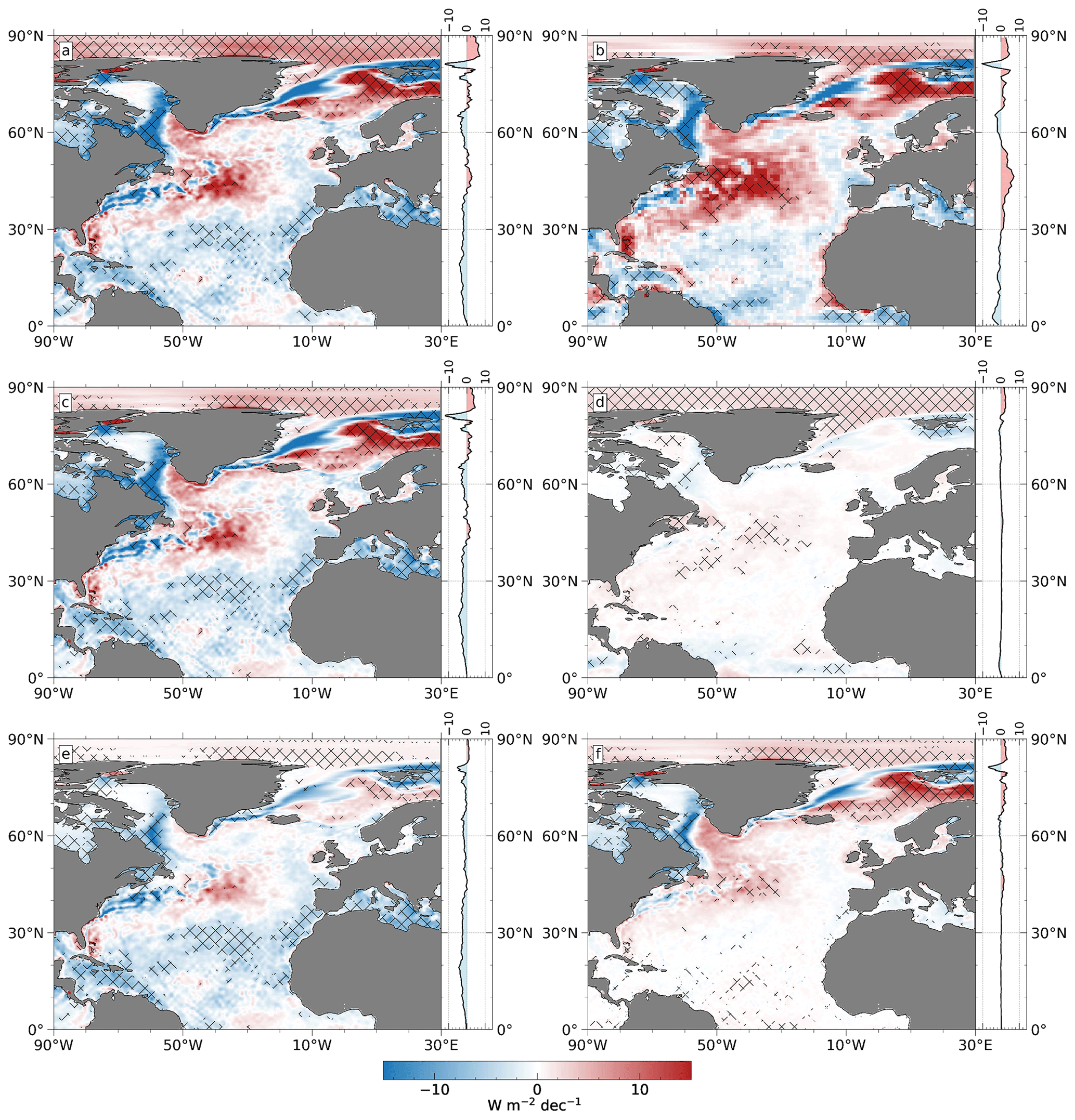
Figure 2Linear trends of (a) model-based FS and (b) inferred FS for the period 1985–2019. Panels (c) and (d) show the turbulent and radiative flux components of model-based FS trends, and panels (e) and (f) illustrate latent and sensible heat fluxes separately. All trends are computed from DJF (December–January–February) means of anomalies. Units are watts per square meter per decade. The shading represents areas of statistically significant trends (95 % confidence level).
Positive trends (weakening of negative net air–sea heat fluxes during winter months) are prominent in the Nordic Seas and in the eastern part of the Labrador Sea, but also in the region where Gulf Stream water masses bifurcate and form the North Atlantic Drift Current further north and the equatorward-propagating Azores Current in the south (between 40–50∘ N and 45–25∘ W). This region of strongly positive trends appears spatially more extended for inferred FS from Mayer et al. (2022) (see Fig. 2b), but with similar peak values of about 29 W m−2 per decade. At other locations of the North Atlantic Ocean, both flux products exhibit qualitatively similar trends, indicating that ERA5 flux trends seem reliable in terms of spatial structure, at least for the chosen study area and period of time. However, note that the trends in many areas are statistically insignificant (e.g., the positive trends in the Labrador and Irminger seas or at the southern flank of the Gulf Stream) and thus should be treated with caution when interpreting them.
The main contributors to the FS trends are turbulent heat fluxes (THFs; Fig. 2c), whereas trends in radiative fluxes (RHFs; Fig. 2d) are usually an order of magnitude weaker (except for the Arctic Ocean, which is not further discussed here). Spatial means over the whole study area are −1.6 W m−2 per decade for THFs and ∼ 0.1 W m−2 per decade for RHFs, resulting in negative FS trends of about −1.4 W m−2 per decade during 1985–2019 (see Table 1). For comparison, the inferred FS exhibits a weak positive trend of 0.3 W m−2 per decade owing to the spatially more extended positive trends.
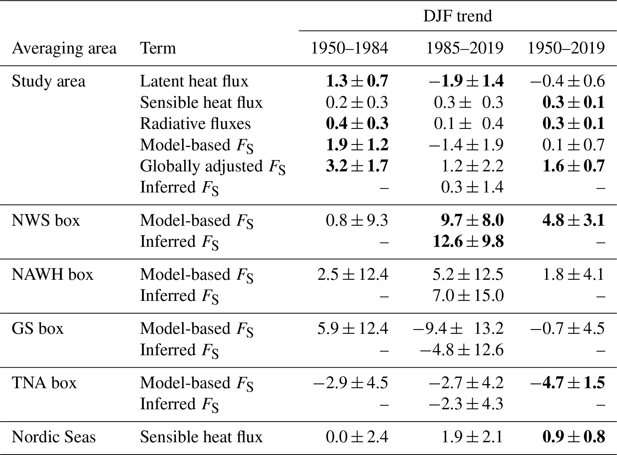
Table 1Flux trends for various areas and periods of time. The study area refers to the ocean area between 0–90∘ N and 90∘ W–30∘ E. The Nordic Seas include the ocean area between 60–82∘ N and 45∘ W–30∘ E. Units are watts per square meter per decade. Bold values are statistically significant trends at the 95 % confidence level. Note that the difference between globally adjusted FS and model-based FS in each period is the magnitude of the global adjustment (see Sect. 3) and can also be added to other model-based FS trend estimates of that particular period.
We also computed mean trends of globally adjusted FS (see Sect. 3) and net air–sea heat fluxes from Liu et al. (2020) (also known as the DEEP-C dataset; publicly available at https://doi.org/10.17864/1947.000347 for the period 1985–2017) over the whole study area. The DEEP-C product is based on our inferred FS, but unrealistic surface fluxes over land are subsequently redistributed to the ocean, which removes spurious trends in the late 1990s and 2000s (Liu et al., 2017, 2020; Mayer et al., 2022). As a consequence, FS from DEEP-C exhibits a realistic global ocean mean that matches the observed mean ocean heat uptake and is thus well suited as a reference for long-term trend studies (Mayer et al., 2022). For 1985–2017, we find a mean trend of 1.4 W m−2 per decade for globally adjusted FS and 1.1 W m−2 per decade for the DEEP-C product (both are statistically insignificant), indicating good agreement of the two estimates. For comparison, the unadjusted model-based FS exhibits a 1985–2017 mean trend of −1.6 W m−2 per decade, indicating that the global adjustment of FS yields more realistic and reliable trend estimates. This adds confidence to our globally adjusted FS data and its use for the full period starting in 1950.
In addition, we show each component of THFs separately. In general, THF trends (and consequently also model-based FS trends) are governed by changes in latent heat flux (Fig. 2e) at low latitudes and sensible heat flux trends (Fig. 2f) at mid-latitudes and high latitudes (north of ∼40∘ N). Of the −1.6 W m−2 per decade mean THF trend, about −1.9 W m−2 per decade stems from latent heat and 0.3 W m−2 per decade from sensible heat flux trends (Table 1). Along the sea ice edge, both components contribute equally to the negative THF trend as both were substantially lower when ocean areas were covered by sea ice before.
While flux trends shown in Fig. 2 are from forecasts, the following evaluations are based on analyzed quantities as they are better constrained by observations than their forecast counterpart. Most differences between forecast and analyzed flux trends can be related to moisture analysis increments (discussed below).
Trends in latent and sensible heat fluxes can further be formally attributed to changes in 10 m horizontal wind speed and temperature or humidity differences between the lowest model level and ocean surface (see bulk formulae Eqs. (1) and (2); trends in air density are not discussed as they are negligibly small). Model-level humidity (Fig. 3a) uniformly increases at almost all locations, as expected from a warming atmosphere (a warmer atmosphere can hold more moisture; Douville et al., 2021). The statistically insignificant decline in the eastern North Atlantic and Mediterranean Sea can be attributed to stronger northerly winds (see Fig. 4a) and declining moisture transport into that area as related to a strengthened NAO.
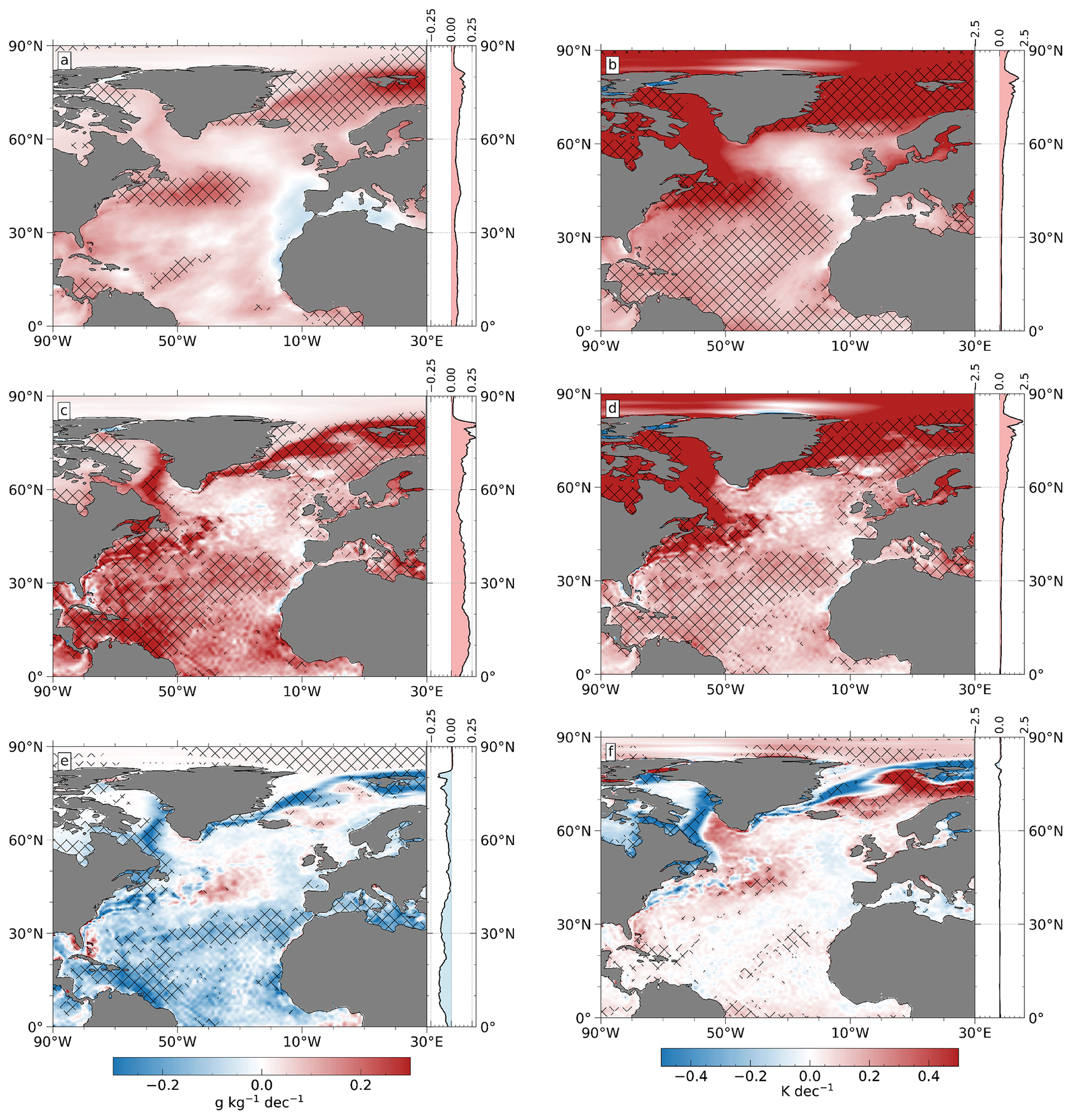
Figure 3Linear DJF trends of analyzed (a) model-level humidity, (b) model-level temperature, (c) surface saturation humidity, and (d) skin temperature anomalies for 1985–2019. In addition, the difference between model-level and surface (e) humidity and (f) temperature is shown. Units are grams per kilogram per decade for humidity trends and kelvin per decade for temperature trends. The shading represents areas of statistically significant trends (95 % confidence level).
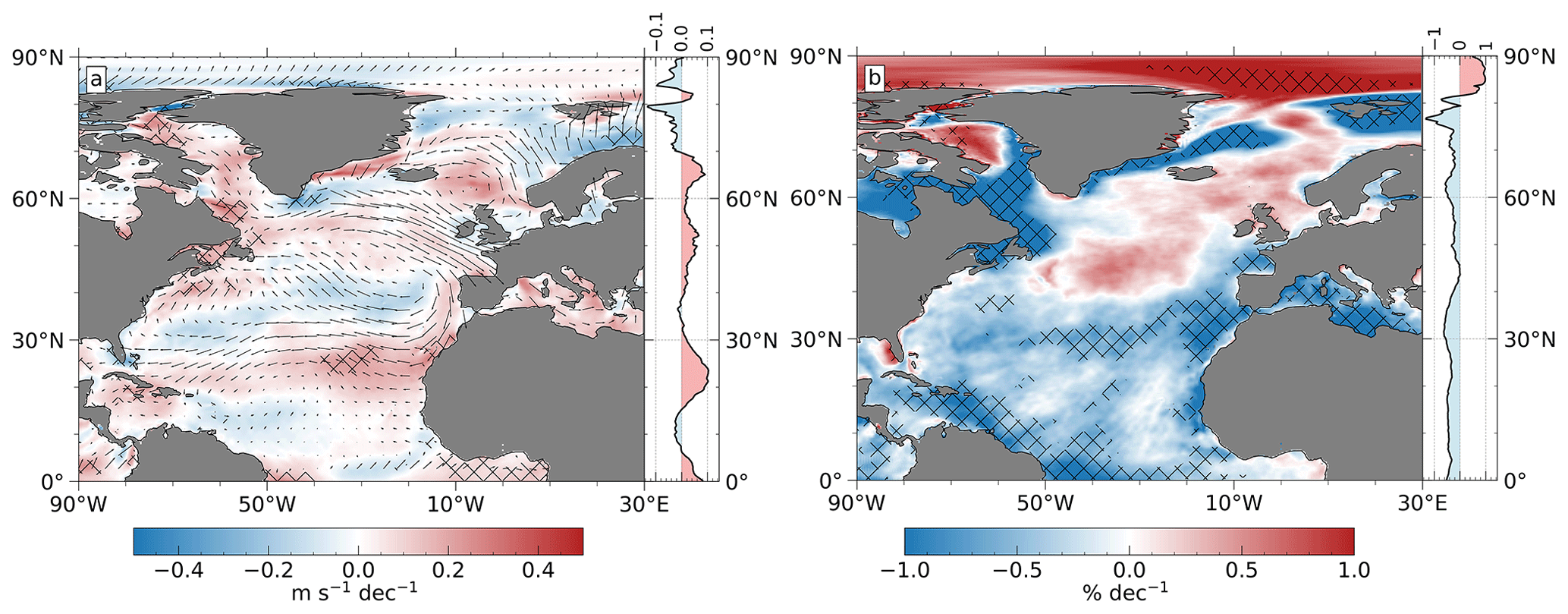
Figure 4Linear trend of analyzed (a) 10 m horizontal wind speed and direction anomalies (m s−1 per decade) and (b) model-level relative humidity (% per decade) for DJF 1985–2019. Anomalous wind direction trends are illustrated by black arrows (with a maximum of ∼ 0.8 m s−1 per decade). The shading represents areas of statistically significant trends (95 % confidence level).
Changes in model-level temperature (Fig. 3b) are qualitatively similar to those in atmospheric moisture but are statistically significant in almost all parts of the tropical North Atlantic. As the ocean warms due to climate change (Fox-Kemper et al., 2021), surface saturation humidity and skin temperature (Fig. 3c and d) increase almost everywhere (note that the surface saturation humidity is derived from skin temperature and surface pressure according to the Clausius–Clapeyron equation). The moderate and statistically insignificant decreasing trend to the south of the Irminger Sea (around 20–30∘ W, 55∘ N), which also appears weaker in model-level variables, is a result of the anomalously cool ocean in the North Atlantic warming hole (Rahmstorf et al., 2015).
The air–sea heat fluxes are not so much governed by individual variables at the surface and model level, but by their differences (Fig. 3e and f), from which several observations can be made:
-
The trend patterns of qml−qsfc and Tml−Tskin are almost identical to that of latent and sensible heat fluxes (cf. Fig. 2e and f; pattern correlations are > 0.8), indicating that the horizontal wind speed (Fig. 4a) has a comparatively small impact on the spatial distribution of latent heat flux (LHF) and sensible heat flux (SHF) trends.
-
Long-term changes in surface saturation humidity (governed by skin temperature trends) are in most areas of the North Atlantic stronger than changes in model-level humidity and vice versa for the temperature. This results in almost uniformly negative qml−qsfc but positive Tml−Tskin trends. While surface saturation humidity increases with increasing skin temperature according to the Clausius–Clapeyron relation (i.e., relative humidity remains 100 %), the increase in model-level humidity is much weaker so that relative humidity decreases (Fig. 4b), especially south of 40∘ N. This means that near-surface air masses in the tropical North Atlantic become drier relative to the temperature increase (the Clausius–Clapeyron relation would postulate stronger humidity trends for constant relative humidity), which can be caused by several factors (discussed below).
-
Among the regions of strong sea ice retreat in the Labrador Sea and Nordic Seas, peak positive trends in surface humidity and temperature can be found along the main current of the Gulf Stream (35–45∘ N, 80–45∘ W; with values up to 0.5 g kg−1 per decade and 0.8 K per decade). This leads to remarkably strong negative trends in qml−qsfc and Tml−Tskin, highlighting the importance of the ocean in this area. It should be noted that the Gulf Stream signal is barely visible in relative humidity trends (Fig. 4b) due to a well-mixed boundary layer and strong coupling between the atmosphere and the underlying warm Gulf Stream.
-
Over the North Atlantic warming hole, changes in the model-level temperature and humidity closely follow the Clausius–Clapeyron relation so that the warming hole signal is barely visible in RH trends (Fig. 4b). Trends in model-level and surface variables are of similar strength, resulting in weak and statistically insignificant heat flux trends (note that the North Atlantic warming hole is further north to the bifurcation area of the Gulf Stream and does not coincide with peak positive trends).
-
The strong positive Tml−Tskin trend in the Norwegian Sea originates from positive trends in the atmosphere and somewhat less positive trends (or even negative trends east of Iceland) of the skin temperature. This can be attributed to trends towards more southeasterly winds (see Fig. 4a) advecting warmer air masses from lower latitudes to the Norwegian Sea, which is related to a strengthened Icelandic Low.
-
In the Labrador Sea and Nordic Seas, Tml−Tskin trends downwind of areas of strong sea ice retreat become widely positive (mean wintertime climatology is a northerly wind in both basins; not shown). One explanation could be that air masses that are advected from further north get heated by the enhanced fluxes where sea ice retreated. The anomalously warm air masses damp air–sea fluxes further south, resulting in largely compensating sensible heat fluxes along the wind direction (spatial average is ∼2 W m−2 per decade over the Nordic Seas; see Table 1), with negative trends in areas of strong sea ice retreat and positive trends downwind. This effect cannot be observed for latent heat fluxes and requires further investigation that is beyond the scope of this study.
One possibility for throttling the growth in near-surface humidity in the tropical North Atlantic is a stronger advection of dry air masses through intensification of the Hadley cell. To manifest this, we present DJF trends of the zonally averaged meridional mass stream function derived from ERA5 wind fields (Fig. 5). The dipole structure between 0–30∘ N indicates that the northern-hemispheric Hadley cell has shifted poleward and strengthened in intensity, which enhances the subsidence of dry air along the northern flank of the Hadley cell. This also agrees with positive trends in 10 m wind speed between ∼20–30∘ N (Fig. 4a). Note that the mass stream function is obtained by integrating over all longitudes, and the intensification may take place over other ocean basins. However, a statistically significant increase in low-level cloud cover and outgoing longwave radiation (not shown; see, e.g., Chen et al., 2002; Mathew and Kumar, 2019) in almost the entire tropical North Atlantic Ocean indicates that the Hadley cell intensification also appears over the tropical Atlantic Ocean.
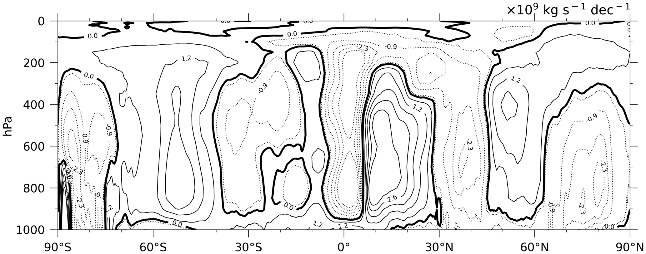
Figure 5Linear trend of the meridional mass stream function from analyzed ERA5 winds over the period 1985–2019. Positive trends are shown as solid contour lines, negative trends as dotted lines. The stream function is integrated over 360∘ in longitude. Units are 109 kg s−1 per decade.
On the other hand, Trenberth et al. (2011) and Mayer et al. (2021) noted that analysis increments introduced by the data assimilation system due to changes in the observing system can artificially remove or add atmospheric moisture, which in turn could influence near-surface humidity trends. To investigate the impact of atmospheric moisture and temperature increments in the lowest model level on air–sea heat fluxes from ERA5, we compute latent and sensible heat fluxes according to the bulk formulas (Eqs. 1 and 2) using both forecast and analyzed state quantities (not shown). Differences between trends derived from analyses and forecasts can then be used as a rough estimate for trend uncertainties caused by analysis increments (note that only temporally varying analysis increments introduce an artificial trend and not a constant offset between analyses and forecasts). It should be highlighted that analysis increments computed in this way cannot be used to fully remove the temporal inconsistencies in model-based FS as their exact impact on both forecasts and analyzed state quantities is unknown. That is, the difference between adjusted and unadjusted model-based FS (magnitude of the global adjustment) is not equivalent to the difference between fluxes computed with forecasts and analyzed state quantities.
We find the strongest variation in humidity increments (approximated by qan−qfc) in the tropics, with values of −0.2 g kg−1 in the late 2000s and early 2010s (see Appendix B) and 1985–2019 trends of about −0.05 g kg−1 per decade. Humidity increments in earlier times and at higher latitudes are in general more stable and less negative. The latent heat flux trends derived from analyses (not shown), for the zonal mean of the North Atlantic, are 1–2 W m−2 per decade more negative than those based on forecasts (root mean square error between trends derived from analysis and forecasts is 1.1 W m−2 per decade over the ice-free ocean). The negative humidity increments in the lowest model level remove moisture from the model, which results in larger qml−qsfc differences and thus stronger (more negative) analyzed latent heat flux trends. For sensible heat fluxes, analysis increments are less important. Temperature increments are temporally more stable and almost independent of latitude, with trends varying between ± 0.03 K per decade (see Appendix B). Zonally averaged SHF trends derived from analyses are less than 0.2 (0.4) W m−2 per decade more positive (negative) at low (high) latitudes than those derived from forecasts (RMSE over the whole study area is 0.5 W m−2 per decade). Consequently, temperature increments are less impactful on turbulent heat fluxes. Trends of turbulent heat fluxes derived from analysis (not shown) are up to 1 W m−2 per decade more negative at all latitudes than those derived from forecasts. However, the spatial pattern of the trends remains almost unaffected because the difference between analyses and forecasts is smaller for weaker trends, and vice versa. Therefore, we argue that the regional impact of all relevant analysis increments introduced by the ERA5 data assimilation on air–sea heat flux trends is rather small during the 1985–2019 period. The negative LHF trends in the tropical North Atlantic are most likely a result of Hadley cell intensification and cannot be explained by temporally varying moisture increments.
In summary, long-term changes in net air–sea heat fluxes over the North Atlantic Ocean are primarily driven by latent heat flux trends (Table 1), which are associated with changes in the surface (related to changes in skin temperature) and model-level humidity (e.g., advection of drier air masses), while changes in wind speed are negligibly small. Furthermore, we conclude that temporally varying analysis increments influence the magnitude of turbulent heat flux trends by about 1 W m−2 per decade, whereas their spatial pattern remains widely unchanged.
4.2 Trends from 1950–1984
Long-term latent and sensible heat flux changes before 1985 (Fig. 6) differ in most areas substantially from those during the more recent period. Most notable are the strong positive and significant LHF trends in the Caribbean Sea, along the Gulf Stream north of ∼ 40∘ N, and in the Labrador Sea.
Trends in sensible heat flux are strongest along the sea ice edge and are absent in the Norwegian Sea, the region with the most prominent negative trends after the 1980s (cf. Fig. 2f). The widely positive trends before 1985 can be attributed to a stronger temperature decrease at the surface relative to the atmosphere (not shown). The skin temperature of the ice-free ocean shows a statistically insignificant increase in wide areas of the tropical North Atlantic and a decrease almost everywhere north of 25∘ N, which coincides with the basin-wide trend pattern of the 0–300 m OHC trend from IAP (not shown). Although their pattern correlation is weak (∼ 0.2) for the ice-free ocean area due to small-scale differences, the generally good match of the large-scale trend pattern in terms of sign suggests that the weakening of sensible heat fluxes is related to the ocean cooling that occurred during that time (see Hodson et al., 2014). For comparison, the pattern correlation for the more recent period 1985–2019, where both skin temperature and OHC increase uniformly (except for the North Atlantic warming hole) due to global warming, is only ∼ 0.15 for the ice-free ocean. This indicates a generally weak spatial correlation between OHC from IAP and skin temperature from ERA5, although their large-scale trend pattern agrees well in terms of sign. As a consequence of the ocean cooling, there is no warming hole signal in the skin and model-level temperature before 1985, which is consistent with results from Chemke et al. (2020) based on satellite-based HadISST data (see supplementary information therein; in fact, ERA5 employs the second version of this dataset as SST forcing; see Hersbach et al., 2020). Temperature analysis increments before 1985 do not play an important role due to their negligibly weak trends of less than ± 0.02 K per decade in ice-free regions. This results in differences between trends derived from analysis and forecast data of less than 0.5 W m−2 per decade in the zonal mean, with an RMSE of about 0.5 W m−2 per decade for the ice-free ocean.
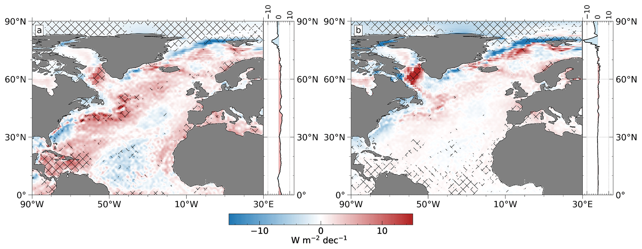
Figure 6As in Fig. 2e and f, but for 1950–1984.
In accordance with the ocean cooling during the 1960s and early 1970s, surface saturation humidity decreases almost everywhere before 1985 (not shown), with the strongest decrease along the Gulf Stream. The only larger patch of positive (but statistically insignificant) trends appears in the subtropics and along the sea ice edge. Near-surface humidity also decreases where temperature decreases (not shown), but weaker than the Clausius–Clapeyron-related decrease such that the relative humidity increases significantly in most areas (whereas negative trends in all ice-free areas are insignificant; not shown). This leads to mostly increasing humidity differences qml−qsfc and thus also in positive latent heat flux trends before 1985 (Fig. 6a).
As for the SHF, we exclude analysis increments as a possible source of uncertainties during that time because of their weak trend of ± 0.02 g kg−1 per decade over most locations of the ice-free ocean. Therefore, differences between LHF trends derived from analyses and forecasts are less then 0.6 W m−2 per decade in zonal mean before 1985 (RMSE over the ice-free ocean is 0.5 W m−2 per decade). Changes in 10 m wind speed are mostly insignificant and of similar strength to that after 1985 and thus affect turbulent heat fluxes only marginally.
4.3 Flux trends in focus regions
To understand long-term changes in the four thermodynamically interesting areas of the North Atlantic (see boxes in Fig. 1) in more detail, we show spatial averages of model-based and inferred FS and partial trends of analyzed input variables as regressed onto LHF and SHF from ERA5 forecasts for the period 1950–2019 (see Fig. 7 and Table 1). In the Norwegian Sea (NWS), air–sea heat fluxes weaken particularly in the late 2000s and 2010s, which is in good agreement with the enhanced oceanic heating during that time (Mork et al., 2019; von Schuckmann et al., 2021). However, the advection of warmer, more humid air associated with changes in 10 m wind direction (see Fig. 4a) appears to dominate oceanic trends (right panel in Fig. 7; partial trends of surface quantities are negative as they contribute with opposite sign to turbulent heat flux trends) so that LHF and SHF trends are relatively weak compared to those in model-level or surface quantities alone. Note that Skagseth et al. (2020) found similar changes in wind direction for the adjacent Barents Sea.
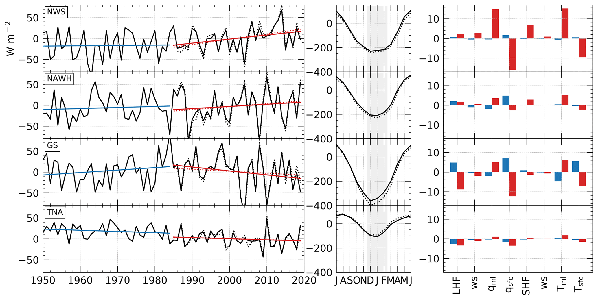
Figure 7(Left) DJF anomalies and (middle) full-year climatology of model-based FS from ERA5 forecasts (solid lines) and inferred FS (dotted lines) for box averages (see Fig. 1) in the Norwegian Sea (NWS), North Atlantic warming hole (NAWH), Gulf Stream (GS), and tropical North Atlantic (TNA). (Right) Partial trends (see Eq. 3) of 10 m wind speed (ws), model-level humidity (qml) and temperature (Tml), surface saturation humidity (qsfc), and skin temperature (Tsfc) as regressed onto latent (LHF) and sensible heat fluxes (SHF), respectively. Climatologies and anomalies are computed with respect to 1985–2019. Trends for 1950–1984 (1985–2019) are shown in blue (red). The gray background in the middle panel highlights the boreal winter months December–February. Units are watts per square meter for anomalies and annual cycles and watts per square meter per decade for trends.
Long-term trends of model-based FS in the North Atlantic warming hole (NAWH) are weak and statistically insignificant in both sub-periods 1950–1984 and 1985–2019 (see also Table 1). Derived trends should thus be treated carefully as they also depend strongly on the chosen reference period. To test the robustness of model-based FS trends in the four study areas, we considered various reference periods. For instance, we removed the last year from the time series and computed DJF trends based on 1950–2018. While net air–sea heat fluxes steadily increase in the NWS and decrease in the tropical North Atlantic (TNA) almost independently of the chosen reference period, trends in the NAWH and GS region are less than 1 W m−2 per decade (or less then 2 W m−2 per decade when considering 1950–2019; see Table 1) and statistically insignificant. From this, we cautiously argue that heat fluxes in the NAWH, and also in the GS box where model-based FS trends from the early and late period compensate each other, do not exhibit a prominent long-term trend over the past 70 years as related to global warming, while changes in the TNA and NWS are most likely a result of global warming.
We also explore the winter-month FS climatology along the Gulf Stream extension on decadal timescales in order to reveal any signal in air–sea heat fluxes associated with a poleward displacement due to global warming. Besides an oscillatory behavior similar to temporal changes in the more regional GS box shown in Fig. 7, we could not find a distinct sign of a poleward shift in air–sea heat fluxes, which is consistent with findings from Yang et al. (2016).
The partial trends in Fig. 7 show that trends in model-level and surface quantities almost always act in opposite directions and thus compensate each other to some degree (except for moisture in the TNA during the first period, where both are negative). In addition, the partial trends demonstrate qualitatively that the impact of 10 m wind speed on heat flux trends is rather small compared to changes in moisture or temperature, especially in cases where latent or sensible heat fluxes exhibit trends of several watts per square meter.
We also find that in the three northernmost boxes, trends of inferred and model-based FS have the same sign but differ by about 2–4 W m−2 per decade. The inferred FS exhibits stronger upward trends in the NWS and NAWH and a weaker downward trend in the GS area (Table 1). Trends in the TNA coincide remarkably well, underlining the reliability of model-based FS in that particular region. In summary, this suggests that model-based trends are largely reliable in terms of sign and spatial pattern (see also Fig. 2).
4.4 Long-term impact of natural variability modes
The North Atlantic Oscillation (NAO) is a periodic oscillation in sea level pressure and wind (Visbeck et al., 2001) and can temporally and regionally influence air–sea interactions. During the last 30–40 years, the NAO tends to more positive phases (strengthened Icelandic Low and Azores High) than before, which has been attributed to global warming (Gillett et al., 2003). Here, we want to explore its long-term impact on trends of air–sea heat fluxes (Fig. 8).
Long-term FS changes over the entire study period appear to be weaker and spatially more uniform compared to those over the two sub-periods discussed before. Trends are widely positive in the western North Atlantic, in the region of the North Atlantic warming hole, and in the Norwegian Sea. Persistent negative flux trends occur in the tropical North Atlantic, along the Gulf Stream, and in regions of strong sea ice retreat which are largely consistent with negative changes during both sub-periods.
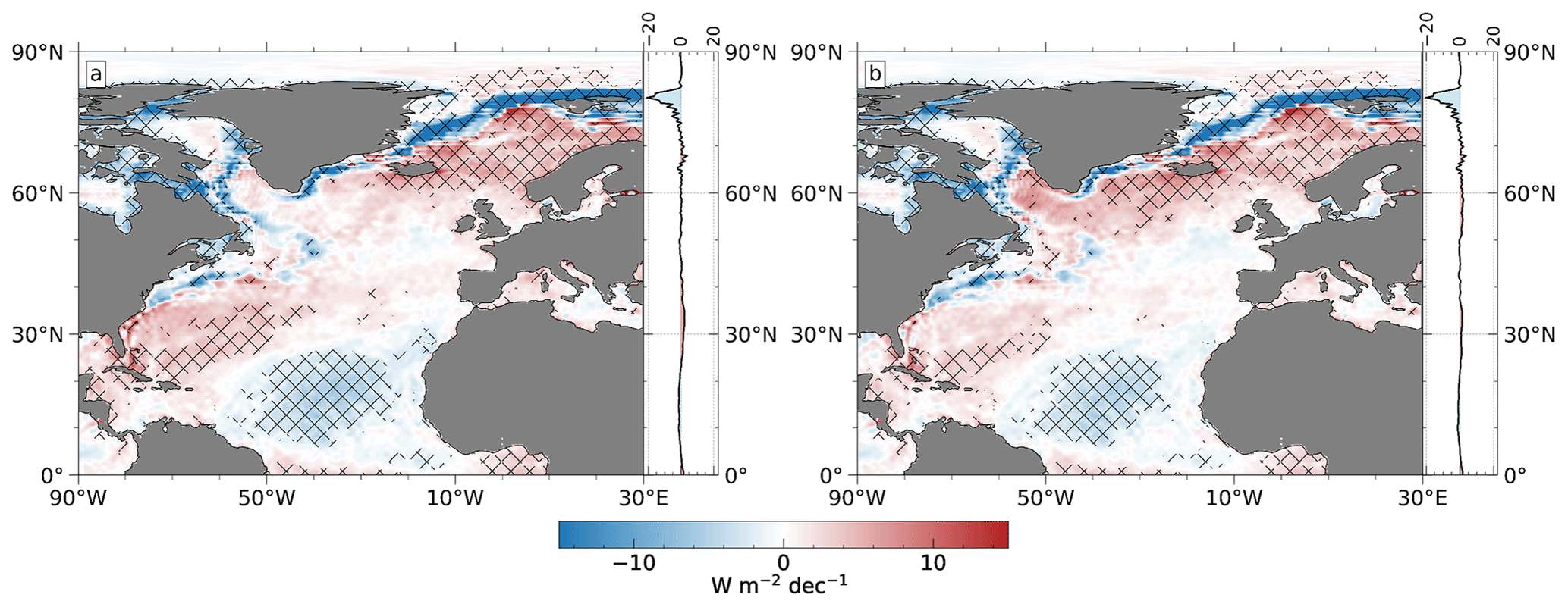
Figure 8(a) Linear trend of model-based FS for 1950–2019, (b) the same but with the partial NAO trend subtracted (see Appendix C for regression pattern). The shading represents areas of statistically significant trends (95 % confidence level).
The December–February NAO regressed onto FS features a basin-wide tripolar pattern (see Appendix C), with strong negative values in the Irminger and Labrador seas, negligibly weak trends in the tropical and subtropical latitudes, and positive values in between (with peak values along the Gulf Stream). The more frequent occurrence of positive NAO phases over the past 30 years, relative to 1950–1990, seem to favor anomalous ocean cooling at higher latitudes and heating in the western North Atlantic (25–45∘ N, 80–40∘ W; see Fig. 8a and positive trends in Fig. C1a). Removing the NAO signal from FS trends (Fig. 8b) thus weakens ocean cooling (more positive trends) in the Irminger and Labrador seas over time and allows stronger cooling in the western North Atlantic (less positive trends). In addition, we find weak correlations of less than 0.4 between NAO index and FS box averages in the TNA, GS, and NWS, but −0.75 for the NAWH. This indicates that the FS trend over the North Atlantic warming hole box is strongly influenced by trends of the NAO and its tendency toward more positive phases, while other areas are less effected.
Despite the remarkably strong regional impact of the NAO on air–sea heat fluxes at high latitudes, its spatial mean averaged over the whole study area is less than 0.03 W m−2 per decade (1950–2019). For comparison, the 1950–2019 FS trend averaged over the whole study area (as shown in Fig. 8a) is 0.14 W m−2 per decade. This suggests that the trend toward more positive NAO phases only leads to a relocation of areas where oceanic heat is lost or taken up through air–sea heat fluxes rather than a steady increase in anomalous ocean heat uptake as related to global warming. This somewhat agrees with the finding of Cohen and Barlow (2005) that the global DJF warming trend during 1972–2004 may be unrelated to regional warming trends driven by the NAO. To check the potential role of decadal NAO variability, we tested the impact of applying locally weighted scatterplot smoothing (LOWESS) and Butterworth low-pass filters on the NAO series before trend computation (not shown), but the impact on the trend results was small, and the results are thus deemed robust.
We also regressed the AMO forcing (Kerr, 2000) onto FS to estimate its long-term impact on flux trends (see Appendix C). The AMO partial trend varies between ± 2 W m−2 per decade over the ice-free ocean, with negative values in the Irminger and Labrador seas and around the North Atlantic warming hole (40–60 and 50–20∘ W) and positive values elsewhere. Although the AMO impact on flux trends in the Irminger and Labrador seas has the same sign and a similar spatial structure to the NAO forcing, its strength over the 70-year period is weaker. Additionally, we find a spatial mean of the AMO signal of 0.22 W m−2 per decade, which points to a basin-wide weakening of air–sea heat fluxes, but this is likely an effect of non-zero AMO trend due to the relative shortness of the time series (the AMO does not complete a full period during the whole study period) and is likely not related to global warming.
4.5 Changes in the Atlantic Meridional Overturning Circulation
In the previous sections we have diagnosed a reduction in the net air–sea heat flux during 1950–2019 when averaging over the North Atlantic. This reduction could be related to a cooling trend of the underlying ocean and/or a reduction in oceanic heat transports associated with the AMOC. In this section we explore both possibilities for verifying the AMOC trends with observation-based data (reanalysis is a combination of observations and forecasts). The ocean heat transport at different latitudes of the North Atlantic basin is indirectly estimated from the ocean heat budget using globally adjusted FS from ERA5 forecasts and OHC data from IAP (see Sect. 3). Here we focus on full-year OHT estimates because it increases the signal-to-noise ratio (sub-annual OHC changes are often related to seasonally compensating trends in wind patterns), and observational uncertainties in OHCT are considered larger on sub-annual timescales. Furthermore, annual mean FS trends are similar to seasonal DJF trends in terms of spatial pattern (pattern correlation is ∼ 0.8) but are generally weaker across the North Atlantic basin (root mean square of trends is 1.8 W m−2 per decade as compared to 3.7 W m−2 per decade).
Results for 0–60∘ N are shown in Fig. 9 using two types of trend estimates (see Sect. 3). Both estimates show more negative trends (weakened AMOC) and larger uncertainties at lower latitudes, with a maximum at the Equator. While the method based on 5-year means gives significant trends for all latitudes except 35–50∘ N (averaging over 5 years reduces the variance), linear regression on monthly data is statistically significant only between 45–60∘ N.
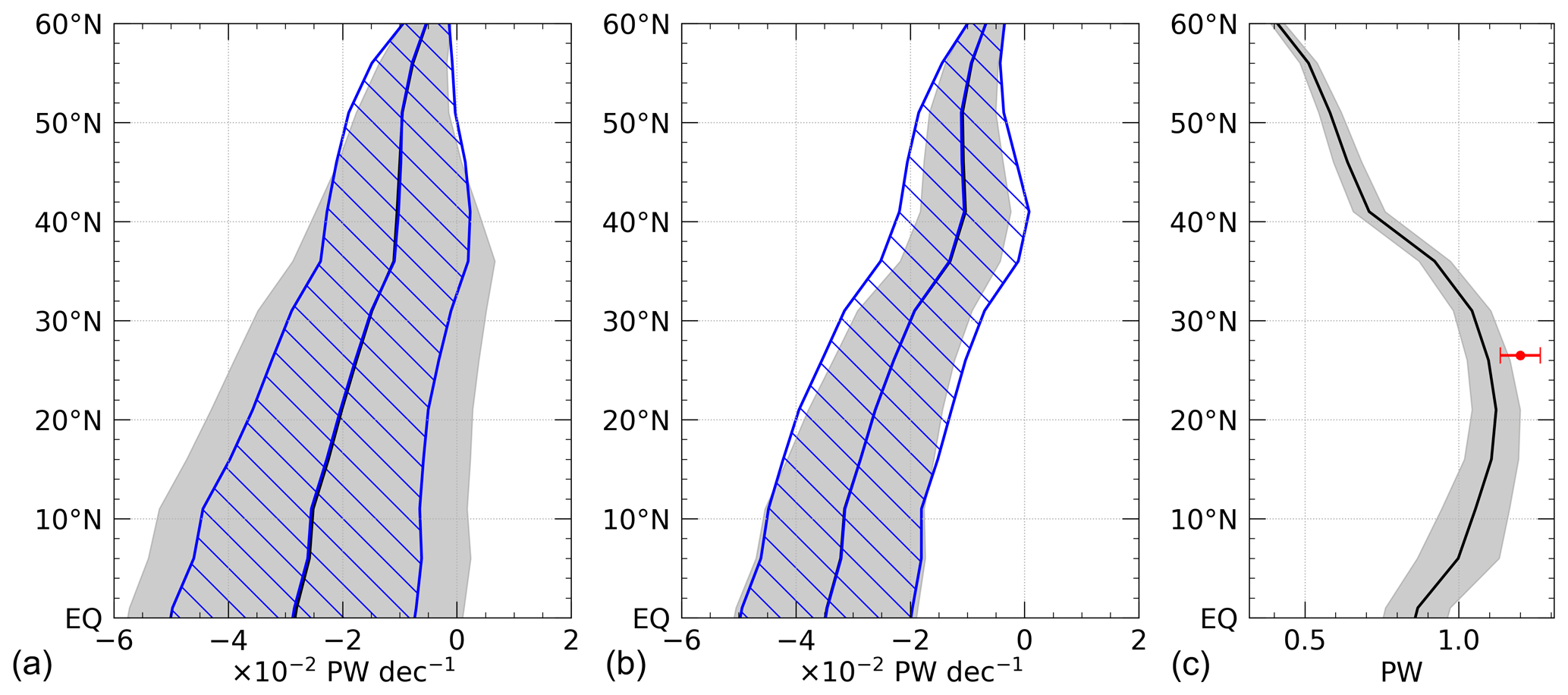
Figure 9(a) The 1950–2019 full-year trend of indirectly estimated Atlantic ocean heat transport as derived from the oceanic heat budget, (b) the same but without OHCT data employed. Blue (gray) lines are trend estimates based on 5-year (monthly) means. The shading illustrates the 95 % confidence interval of the trend estimate. (c) The 1950–2019 mean total indirectly estimated heat transport at each latitude. The red dot shows the 2004–2018 mean observed ocean heat transport through the RAPID array at 26.5∘ N.
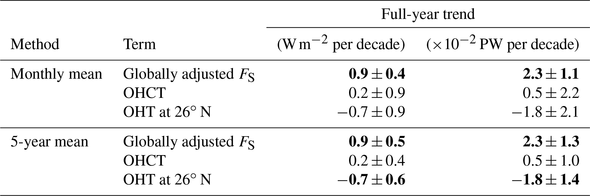
The main contributors to the weakened OHT in the North Atlantic basin are statistically significant long-term changes in globally adjusted air–sea heat fluxes, whereas the trend of meridionally integrated OHCT is comparably small and insignificant throughout all latitudes between the Equator and 60∘ N (see Table 2 for trends integrated over the area between the choke point DS + FS + BSO and 26∘ N). Removing the OHCT term from the budget equation (integral term in Eq. 5) thus reduces trend uncertainties, while the strength and meridional structure of the estimated OHT trend remain roughly the same (compare left and middle panel of Fig. 9). In other words, the AMOC weakening is primarily associated with a positive trend of globally adjusted FS and thus a decline in ocean-to-atmosphere heat fluxes (1950–2019 mean is −13.7 W m−2). We also computed the indirectly estimated OHT trend based on the sub-periods 1950–1984 and 1985–2019 but could not find a significant AMOC weakening in either period (not shown).
Table 2Full-year trends of globally adjusted air–sea heat fluxes from ERA5 forecasts, ocean heat content tendency (OHCT), and indirectly estimated ocean heat transport (OHT) at 26∘ N for the period 1950–2019. FS and OHCT are spatially integrated over the ocean area between the choke point in the north (see red lines in Fig. 1) and 26∘ N. Trends are estimated based on full-year monthly means and 5-year means. Bold values are statistically significant trends at the 95 % confidence level. The left column contains area-averaged values (relative to the area between the northern choke point and 26∘ N) given in watts per square meter per decade. The values in the right column represent the area-integrated contribution to the ocean heat budget given in petawatts per decade.
In this work, we investigated the reliability and temporal stability of winter-month (December–February) trends of model-based net air–sea heat fluxes from ERA5 forecasts (denoted as model-based FS) over the North Atlantic Ocean during 1950–2019. Main drivers of these trends are identified using analyzed state quantities from ERA5, and the influence of natural variability modes and analysis increments as introduced by the ERA5 data assimilation system is considered. Whenever possible, ERA5 forecast fluxes are compared with indirect estimates from Mayer et al. (2022), which are proven to be temporally stable and exhibit a small mean bias over the global ocean. Furthermore we performed a linear perturbation analysis on turbulent heat fluxes in four distinct 8 × 8∘ boxes, which allowed us to quantitatively attribute flux trends to changes in wind speed, moisture, and temperature, assuming a linear regime. In a final step, we used basin-wide annual mean air–sea heat fluxes to indirectly estimate the AMOC trends over the past 70 years and discussed their reliability and sources of uncertainties.
We find that air–sea heat flux trends at low (high) latitudes are largely driven by long-term changes in differences between model-level and surface humidity (temperature). We further traced surface trends back to local changes in the ocean heat content, whereas model level trends strongly depend on altered conditions of advected air masses through changes in wind direction and not so much in wind speed. This process likely plays a major role in the tropical North Atlantic, where increasingly drier air masses are advected (likely linked with a strengthening of the Hadley cell), as well as in the Norwegian Sea, where increasingly warmer air is advected.
A more quantitative assessment of turbulent heat fluxes in four individual sub-regions reveals that the relative contribution of wind speed to turbulent heat flux trends is indeed negligible and that surface and model level trends largely compensate each other. Furthermore, it is shown that trends in the later period (1985–2019) are substantially stronger compared to the early period, which is consistent with accelerated warming in the past few decades (Cheng et al., 2017; Fox-Kemper et al., 2021). It should be noted that the strength of trends clearly depends on the chosen averaging area, especially in the Gulf Stream, where north–south gradients of air–sea heat flux trends are steep.
The long-term changes in air–sea heat fluxes could have some further implications on weather and climate. For instance, the increased intensity of tropical cyclones during the past 40 years (Kossin et al., 2020) could possibly be linked to stronger latent heat fluxes in the tropical North Atlantic (Fig. 2e; similar trends can be found for the hurricane season, September–November). Similarly, the negative heat flux trends over the Gulf Stream are most likely a response to an increased storm frequency, which as a further consequence favors more cyclogenesis (Shaman et al., 2010).
We also examined the impact of NAO and AMO on long-term FS trends. The more frequent positive NAO phases during the last 30–40 years significantly alter trends at high latitudes. It favors stronger ocean heat loss to the atmosphere via air–sea heat fluxes in the Irminger and Labrador seas and anomalously weak loss in the western North Atlantic, although the basin-wide mean heat exchange between the atmosphere and ocean remains unaffected. The AMO forcing, on the other hand, is weaker than the NAO forcing but exhibits a non-zero mean in the North Atlantic basin, but robust statements about the impact of AMO are difficult given the relative shortness of the considered time series.
Finally, we linked the basin-wide air–sea heat flux trend to the AMOC weakening found in other studies by evaluating the oceanic heat budget using air–sea heat fluxes from ERA5 forecasts, OHCT data from IAP, and ocean heat transport data from Arctic gateways in the north (i.e., mooring-derived estimates from the Davis Strait, Fram Strait, and Barents Sea opening; see Fig. 1). As 90 % of the observed total meridional heat transport at 26∘ N is carried out by the overturning circulation (Johns et al., 2011; Zhang et al., 2019), the found decrease in inferred OHT can be directly linked to a weakening of the AMOC. Trend estimates based on monthly data exhibit large uncertainties and are insignificant south of 45∘ N, whereas computations based on 5-year means yield significant trends at almost all latitudes (taking into account all significant autocorrelation coefficients; see Sect. 3). Removing the OHCT term from the calculations reduces uncertainties, while trends remain approximately the same (the long-term OHCT trend is small compared to that in FS but introduces noise). Based on these results, we provide new and independent evidence for a weakening of the AMOC over the past 70 years (see also Rahmstorf et al., 2015; Caesar et al., 2018; Fox-Kemper et al., 2021; Boers, 2021), which is associated with positive heat flux trends (weakened negative fluxes) in the North Atlantic basin. We argue that the mean ocean heat transport through the choke point in the Nordic Seas is small (∼ 0.15 PW) so that even relatively large changes would not have a strong impact on indirectly estimated OHT trends further south (see Muilwijk et al., 2018, for long-term simulations of ocean heat transports through Arctic gateways).
Analysis increments of moisture and temperature at the lowest model level (i.e., the difference between analysis and forecast) likely influence the strength of trends but not so much the basin-wide spatial pattern. At most locations, moisture is removed from the model by the assimilation process, resulting in stronger (more negative) LHF trends from analyzed data by about 1 W m−2 per decade as compared to forecast data. The strongest moisture analysis increments can be found in the tropics in the late 2000s. At higher latitudes and before 2000, moisture increments are temporally stable and have a negligible impact on turbulent air–sea heat flux trends. Temperature increments are relatively small and stable throughout the study period and thus play only a secondary role.
In the early period, observations are temporally and spatially sparse, resulting in analyzed states that are closer to the model climate (to which forecasts are drifting) than to observations. Over time, more and more observational data are assimilated, pulling the analysis away from the model climate. This increases analysis increments, which can have several implications on air–sea heat flux trend estimates. When trends are weak or compensate each other such that the signal-to-noise ratio becomes low (e.g., when averaging over large areas), analysis increments can have a relatively large impact on the trend estimate. For example, the heat flux trend in the tropical North Atlantic box (see Fig. 1) is only −2.7 W m−2 per decade during 1985–2019 (Table 1). Analysis increments increasingly remove moisture from the atmosphere in that region (see Appendix B) so that the trend based on analyzed state quantities is −4 W m−2 per decade (not shown). This is a 50 % stronger trend compared to the forecast-based estimate. Nonetheless, it is important to note that this is still a factor of ∼ 3 smaller than the trend uncertainty listed in Table 1. A similar effect can be found for global ocean and basin-wide averages, as used to estimate the AMOC weakening. Both suffer from temporal inconsistencies in the late 1990s and early 2000s, which are likely caused by changes in the atmospheric observing system and hence analysis increments. Nevertheless, given that trends in analysis increments are spatially relatively uniform, we find that the applied global correction removes much of the effect of the spurious air–sea flux trend on our inferred estimate of OHT; that is, temporal inconsistencies in basin-wide averages of model-based FS (and thus also in the inferred OHT) are almost completely eliminated by the global correction.
From our results, we find that analysis increments are a useful tool for interpreting the trend estimates based on reanalysis data. Air–sea heat flux trends from ERA5 forecasts in the North Atlantic basin seem reliable in terms of sign (on sub-basin scale; see Fig. 7) and spatial structure, but we speculate that temporal inconsistencies in the late 1990s and 2000s (as shown by Mayer et al., 2022, for global ocean averages) and temporally varying analysis increments have a common cause, which is the increasing number of observations that indicate a drier atmosphere than in the model climate. Further research is needed to fully understand their impact on both forecast- and analysis-based trends.
Turbulent heat fluxes are linearized by decomposing each variable on the right side of Eqs. (1) and (2) into a mean state (with overbar) and deviation from the mean (with prime); that is, we substitute , , , and , where , and . After some calculus, turbulent heat fluxes can be separated into a non-linear and linear part, where the former contains all products with more than one deviation term (e.g., the non-linear term ; not shown). The linear latent heat flux can be written as
and the linear sensible heat flux as
Figure B1 shows 1985–2019 trends of moisture and temperature increments and corresponding TNA box averages for the whole study period. Note that moisture increments in the tropical North Atlantic before 2000 are remarkably stable around zero but rapidly decrease afterward, with minimum values of about −0.2 g kg−1 in 2010–2015 (negative analysis increments mean that moisture is removed from the model by the data assimilation). Temperature increments show a weak increase in the early 1990s but are temporally stable between 0–0.1 K otherwise.
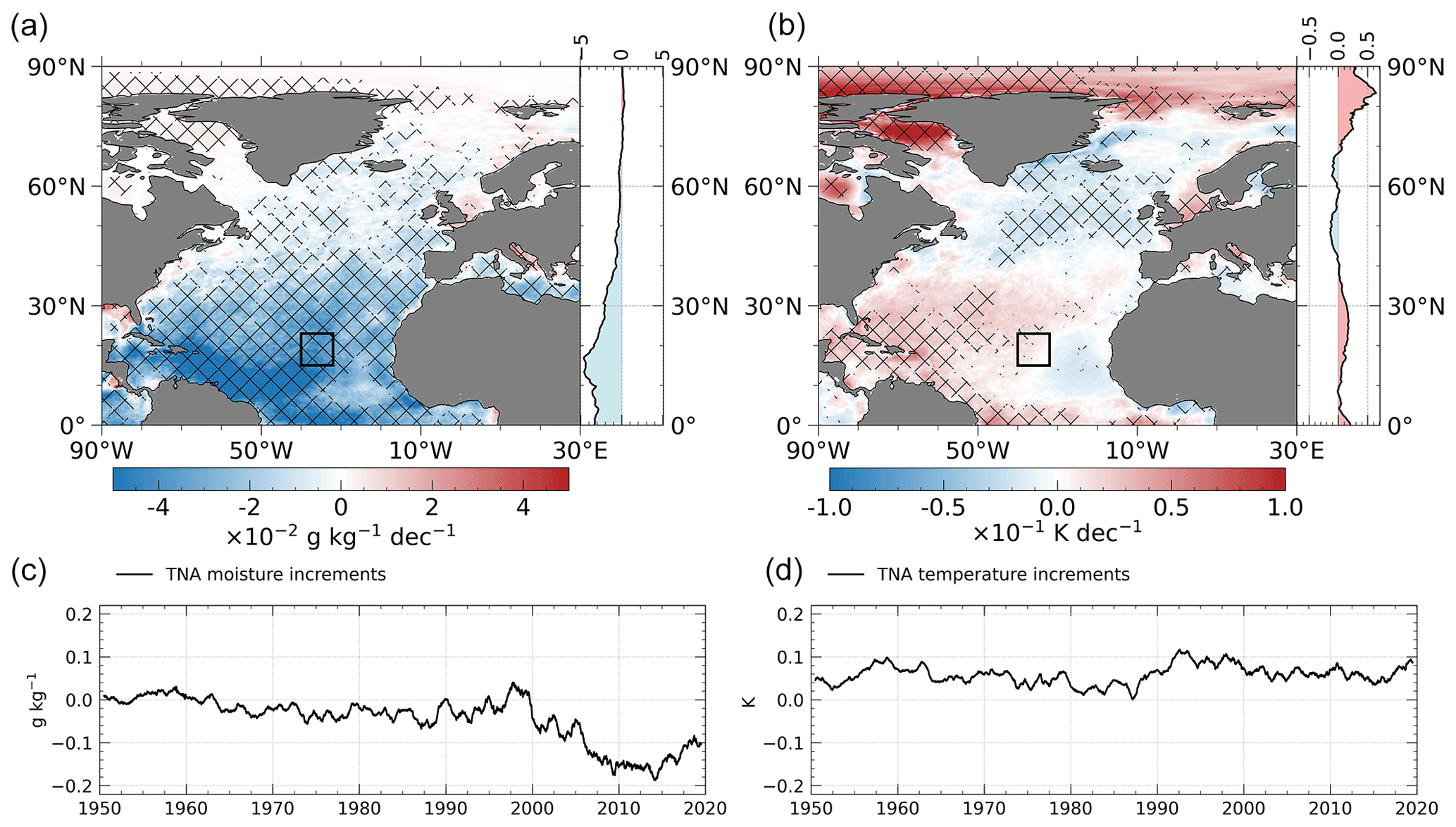
Figure B1Analysis increments (analysis minus forecast field) of (a) moisture and (c) temperature at the lowest model level. The upper panel shows DJF trend maps of analysis increments for the period 1985–2019. The lower panel shows analysis increments of the TNA box average for the whole study period. Time series are smoothed by a 12-month moving average.
Figure C1 shows winter-month partial trends of NAO and AMO as regressed onto air–sea heat fluxes from ERA5 forecasts for the period 1950–2019.
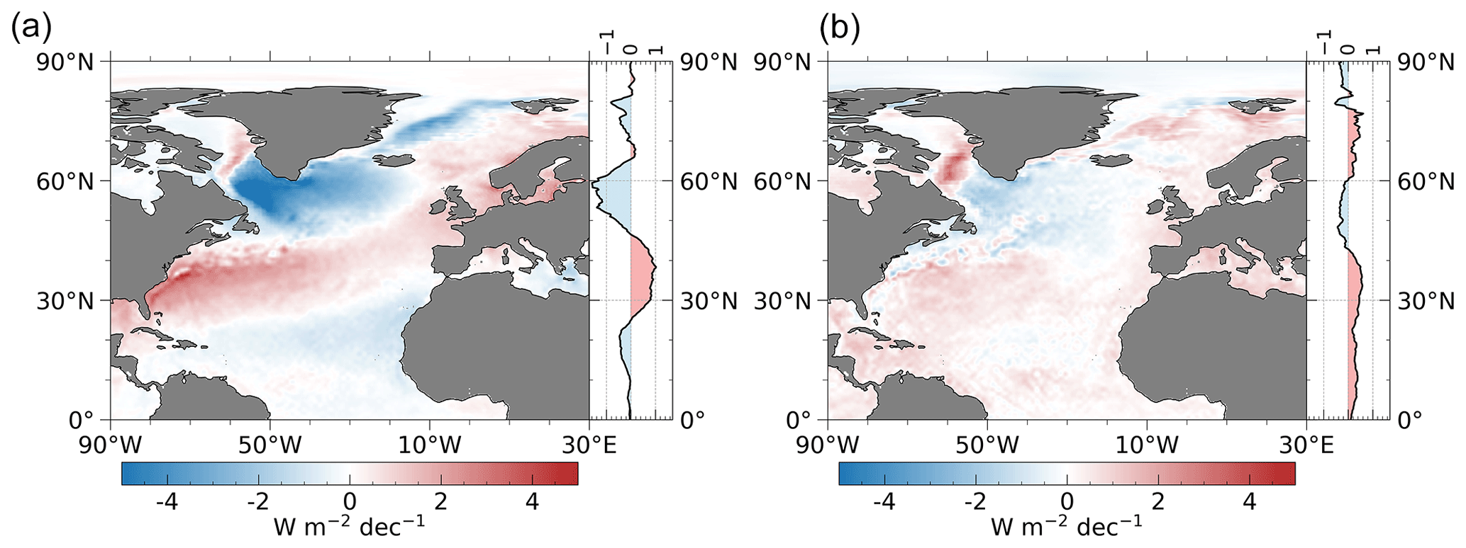
Figure C1Partial trends of (a) NAO and (b) AMO as regressed onto air–sea heat fluxes from ERA5 forecasts for the period 1950–2019. Partial trends are computed for each grid point by multiplying the sensitivity between climate index and FS with the linear trend of the climate index (see explanation to Eq. 3).
The source code used for this study is available at https://doi.org/10.5281/zenodo.10017792 (Mayer, 2023).
ERA5 data are publicly available through the Copernicus Climate Data Store (Hersbach et al., 2023). Atmospheric energy transport and storage terms are also publicly available through the Copernicus Climate Data Store; see Mayer et al. (2022b). Ocean heat content data are provided by the Institute of Atmospheric Physics and are freely accessible at ftp://www.ocean.iap.ac.cn/cheng/IAP_Ocean_heat_content_0_2000m/ (Cheng et al., 2017; last access: 27 August 2023). Ocean heat transport estimates from the moored buoy array in the Arctic gateways are available at https://metadata.nmdc.no/metadata-api/landingpage/0a2ae0e42ef7af767a920811e83784b1 (Tsubouchi et al., 2018; last access: 27 August 2023) and https://doi.org/10.1594/PANGAEA.909966 (Tsubouchi et al., 2020; last access: 27 August 2023).
All authors participated in the discussion and conceptual design of the paper. JM prepared the figures and wrote the manuscript under the supervision of LH and MM.
The contact author has declared that none of the authors has any competing interests.
Publisher’s note: Copernicus Publications remains neutral with regard to jurisdictional claims made in the text, published maps, institutional affiliations, or any other geographical representation in this paper. While Copernicus Publications makes every effort to include appropriate place names, the final responsibility lies with the authors.
Johannes Mayer and Michael Mayer were financially supported by the Austrian Science Funds (FWF) project P33177. Leopold Haimberger received support from the Austrian HRSM project GEOCLIM.
Johannes Mayer and co-author Michael Mayer were funded by the FWF project P33177. Leopold Haimberger received support from the Austrian HRSM project GEOCLIM.
This paper was edited by Jadranka Sepic and reviewed by two anonymous referees.
Baehr, J., Haak, H., Alderson, S., Cunningham, S. A., Jungclaus, J. H., and Marotzke, J.: Timely Detection of Changes in the Meridional Overturning Circulation at 26∘ N in the Atlantic, J. Clim., 20, 5827–5841, https://doi.org/10.1175/2007JCLI1686.1, 2007. a
Baker, J. A., Renshaw, R., Jackson, L. C., Dubois, C., Iovino, D., Zuo, H., Perez, R. C., Dong, S., Kersalé, M., Mayer, M., Mayer, J., Speich, S., and Lamont, T.: Overturning and heat transport variations in the South Atlantic in an ocean reanalysis ensemble, State Planet, 1-osr7, 4 pp., https://doi.org/10.5194/sp-1-osr7-4-2023, 2022. a
Bell, B., Hersbach, H., Simmons, A., Berrisford, P., Dahlgren, P., Horányi, A., Muñoz-Sabater, J., Nicolas, J., Radu, R., Schepers, D., Soci, C., Villaume, S., Bidlot, J.-R., Haimberger, L., Woollen, J., Buontempo, C., and Thépaut, J.-N.: The ERA5 global reanalysis: Preliminary extension to 1950, Q. J. Roy. Meteor. Soc., 147, 4186–4227, https://doi.org/10.1002/qj.4174, 2021. a
Bengtsson, L., Hagemann, S., and Hodges, K. I.: Can climate trends be calculated from reanalysis data?, J. Geophys. Res.-Atmos., 109, D11111, https://doi.org/10.1029/2004JD004536, 2004. a
Boers, N.: Observation-based early-warning signals for a collapse of the Atlantic Meridional Overturning Circulation, Nat. Clim. Change, 11, 680–688, https://doi.org/10.1038/s41558-021-01097-4, 2021. a
Bryden, H. L., Johns, W. E., King, B. A., McCarthy, G., McDonagh, E. L., Moat, B. I., and Smeed, D. A.: Reduction in Ocean Heat Transport at 26∘ N since 2008 Cools the Eastern Subpolar Gyre of the North Atlantic Ocean, J. Clim., 33, 1677–1689, https://doi.org/10.1175/JCLI-D-19-0323.1, 2020. a
Caesar, L., Rahmstorf, S., Robinson, A., Feulner, G., and Saba, V.: Observed fingerprint of a weakening Atlantic Ocean overturning circulation, Nature, 556, 191–196, https://doi.org/10.1038/s41586-018-0006-5, 2018. a
Chemke, R., Zanna, L., and Polvani, L. M.: Identifying a human signal in the North Atlantic warming hole, Nat. Commun., 11, 1–7, 2020. a
Chen, J., Carlson, B. E., and Genio, A. D. D.: Evidence for Strengthening of the Tropical General Circulation in the 1990s, Science, 295, 838–841, https://doi.org/10.1126/science.1065835, 2002. a
Cheng, L. and Zhu, J.: Benefits of CMIP5 Multimodel Ensemble in Reconstructing Historical Ocean Subsurface Temperature Variations, J. Clim., 29, 5393–5416, https://doi.org/10.1175/JCLI-D-15-0730.1, 2016. a
Cheng, L., Trenberth, K. E., Fasullo, J., Boyer, T., Abraham, J., and Zhu, J.: Improved estimates of ocean heat content from 1960 to 2015, Sci. Adv., 3, e1601545, https://doi.org/10.1126/sciadv.1601545, 2017. a, b, c, d
Chiodo, G. and Haimberger, L.: Interannual changes in mass consistent energy budgets from ERA-Interim and satellite data, J. Geophys. Res.-Atmos., 115, D02112, https://doi.org/10.1029/2009JD012049, 2010. a
Cohen, J. and Barlow, M.: The NAO, the AO, and Global Warming: How Closely Related?, J. Clim., 18, 4498–4513, https://doi.org/10.1175/JCLI3530.1, 2005. a
Cronin, M. F., Gentemann, C. L., Edson, J., Ueki, I., Bourassa, M., Brown, S., Clayson, C. A., Fairall, C. W., Farrar, J. T., Gille, S. T., Gulev, S., Josey, S. A., Kato, S., Katsumata, M., Kent, E., Krug, M., Minnett, P. J., Parfitt, R., Pinker, R. T., Stackhouse, P. W., Swart, S., Tomita, H., Vandemark, D., Weller, A. R., Yoneyama, K., Yu, L., and Zhang, D.: air-sea Fluxes With a Focus on Heat and Momentum, Front. Mar. Sci., 6, 430, https://doi.org/10.3389/fmars.2019.00430, 2019. a
Docquier, D. and Koenigk, T.: A review of interactions between ocean heat transport and Arctic sea ice, Environ. Res. Lett., 16, 123002, https://doi.org/10.1088/1748-9326/ac30be, 2021. a
Douville, H., Raghavan, K., Renwick, J., Allan, R., Arias, P., Barlow, M., Cerezo-Mota, R., Cherchi, A., Gan, T., Gergis, J., Jiang, D., Khan, A., Mba, W. P., Rosenfeld, D., Tierney, J., and Zolina, O.: Water Cycle Changes, Climate Change 2021: The Physical Science Basis. Contribution of Working Group I to the Sixth Assessment Report of the Intergovernmental Panel on Climate Change, Cambridge University Press, 1055–1210, https://doi.org/10.1017/9781009157896.010, 2021. a
ECMWF: IFS Documentation CY47R3 – Part IV Physical processes, ECMWF, 1–232, https://doi.org/10.21957/eyrpir4vj, 2021. a, b, c
Fairall, C. W., Bradley, E. F., Hare, J. E., Grachev, A. A., and Edson, J. B.: Bulk Parameterization of Air–Sea Fluxes: Updates and Verification for the COARE Algorithm, J. Clim., 16, 571–591, https://doi.org/10.1175/1520-0442(2003)016<0571:BPOASF>2.0.CO;2, 2003. a
Fasullo, J. T. and Trenberth, K. E.: The Annual Cycle of the Energy Budget, Part I: Global Mean and Land–Ocean Exchanges, J. Clim., 21, 2297–2312, https://doi.org/10.1175/2007JCLI1935.1, 2008. a
Fox-Kemper, B., Hewitt, H., Xiao, C., Aðalgeirsdóttir, G., Drijfhout, S., Edwards, T., Golledge, N., Hemer, M., Kopp, R., Krinner, G., Mix, A., Notz, D., Nowicki, S., Nurhati, I., Ruiz, L., Sallée, J.-B., Slangen, A., and Yu, Y.: Ocean, Cryosphere and Sea Level Change, Climate Change 2021: The Physical Science Basis. Contribution of Working Group I to the Sixth Assessment Report of the Intergovernmental Panel on Climate Change, Cambridge University Press, 1211–1362, https://doi.org/10.1017/9781009157896.011, 2021. a, b, c, d, e, f
Gillett, N. P., Graf, H. F., and Osborn, T. J.: Climate Change and the North Atlantic Oscillation, American Geophysical Union (AGU), 193–209, https://doi.org/10.1029/134GM09, 2003. a
Hersbach, H., Bell, B., Berrisford, P., Hirahara, S., Horányi, A., Muñoz-Sabater, J., Nicolas, J., Peubey, C., Radu, R., Schepers, D., Simmons, A., Soci, C., Abdalla, S., Abellan, X., Balsamo, G., Bechtold, P., Biavati, G., Bidlot, J., Bonavita, M., De Chiara, G., Dahlgren, P., Dee, D., Diamantakis, M., Dragani, R., Flemming, J., Forbes, R., Fuentes, M., Geer, A., Haimberger, L., Healy, S., Hogan, R. J., Hólm, E., Janisková, M., Keeley, S., Laloyaux, P., Lopez, P., Lupu, C., Radnoti, G., de Rosnay, P., Rozum, I., Vamborg, F., Villaume, S., and Thépaut, J.-N.: The ERA5 Global Reanalysis, Q. J. Roy. Meteorol. Soc., 146, 1999–2049, https://doi.org/10.1002/qj.3803, 2020. a, b, c, d, e
Hersbach, H., Bell, B., Berrisford,, P., Hirahara, S., Horányi, A., Muñoz‐Sabater, J., Nicolas, J., Peubey, C., Radu, R., Schepers, D., Simmons, A., Soci, C., Abdalla, S., Abellan, X., Balsamo, G., Bechtold, P., Biavati, G., Bidlot, J., Bonavita, M., De Chiara, G., Dahlgren, P., Dee, D., Diamantakis, M., Dragani, R., Flemming, J., Forbes, R., Fuentes, M., Geer, A., Haimberger, L., Healy, S., Hogan, R., Hólm, E., Janisková, M., Keeley, S., Laloyaux, P., Lopez, P., Lupu, C., Radnoti, G., de Rosnay, P., Rozum, I., Vamborg, F., Villaume, S., and Thépaut, J.-N.: Complete ERA5 global atmospheric reanalyis: Fifth generation of ECMWF atmospheric reanalyses of the global climate [data set], https://doi.org/10.24381/CDS.143582CF, 2023. a, b
Hodson, D. L. R., Robson, J. I., and Sutton, R. T.: An Anatomy of the Cooling of the North Atlantic Ocean in the 1960s and 1970s, J. Clim., 27, 8229–8243, https://doi.org/10.1175/JCLI-D-14-00301.1, 2014. a
Hurrell, J. W.: Decadal Trends in the North Atlantic Oscillation: Regional Temperatures and Precipitation, Science, 269, 676–679, https://doi.org/10.1126/science.269.5224.676, 1995. a, b
Hurrell, J. W. and Deser, C.: North Atlantic climate variability: The role of the North Atlantic Oscillation, J. Mar. Syst., 78, 28–41, https://doi.org/10.1016/j.jmarsys.2008.11.026, 2009. a
Johns, W. E., Baringer, M. O., Beal, L. M., Cunningham, S. A., Kanzow, T., Bryden, H. L., Hirschi, J. J. M., Marotzke, J., Meinen, C. S., Shaw, B., and Curry, R.: Continuous, Array-Based Estimates of Atlantic Ocean Heat Transport at 26.5∘ N, J. Clim., 24, 2429–2449, https://doi.org/10.1175/2010JCLI3997.1, 2011. a, b
Kerr, R. A.: A North Atlantic Climate Pacemaker for the Centuries, Science, 288, 1984–1985, https://doi.org/10.1126/science.288.5473.1984, 2000. a, b
Kossin, J. P., Knapp, K. R., Olander, T. L., and Velden, C. S.: Global increase in major tropical cyclone exceedance probability over the past four decades, P. Natl. Acad. Sci. USA, 117, 11975–11980, https://doi.org/10.1073/pnas.1920849117, 2020. a
Liu, C., Allan, R. P., Mayer, M., Hyder, P., Loeb, N. G., Roberts, C. D., Valdivieso, M., Edwards, J. M., and Vidale, P.-L.: Evaluation of satellite and reanalysis-based global net surface energy flux and uncertainty estimates, J. Geophys. Res.-Atmos., 122, 6250–6272, https://doi.org/10.1002/2017JD026616, 2017. a, b
Liu, C., Allan, R. P., Mayer, M., Hyder, P., DesbruyÈres, D., Cheng, L., Xu, J., Xu, F., and Zhang, Y.: Variability in the global energy budget and transports 1985–2017, Clim. Dynam., 55, 3381–3396, https://doi.org/10.1007/s00382-020-05451-8, 2020. a, b, c, d, e
Liu, C., Yang, Y., Liao, X., Cao, N., Liu, J., Ou, N., Allan, R. P., Jin, L., Chen, N., and Zheng, R.: Discrepancies in Simulated Ocean Net Surface Heat Fluxes over the North Atlantic, Adv. Atmos. Sci., 39, 1941–1955, https://doi.org/10.1007/s00376-022-1360-7, 2022. a
Loeb, N. G., Mayer, M., Kato, S., Fasullo, J. T., Zuo, H., Senan, R., Lyman, J. M., Johnson, G. C., and Balmaseda, M.: Evaluating Twenty-Year Trends in Earth's Energy Flows From Observations and Reanalyses, J. Geophys. Res.-Atmos., 127, e2022JD036686, https://doi.org/10.1029/2022JD036686, 2022. a
Mathew, S. S. and Kumar, K. K.: Characterization of the long-term changes in moisture, clouds and precipitation in the ascending and descending branches of the Hadley Circulation, J. Hydrol., 570, 366–377, https://doi.org/10.1016/j.jhydrol.2018.12.047, 2019. a
Mayer, J.: Source code for 10.5194/esd-2023-8, Zenodo [code], https://doi.org/10.5281/zenodo.10017792, 2023. a
Mayer, J., Mayer, M., and Haimberger, L.: Consistency and Homogeneity of Atmospheric Energy, Moisture, and Mass Budgets in ERA5, J. Clim., 34, 3955–3974, https://doi.org/10.1175/JCLI-D-20-0676.1, 2021. a, b, c, d, e, f, g
Mayer, J., Mayer, M., Haimberger, L., and Liu, C.: Comparison of Surface Energy Fluxes from Global to Local Scale, J. Clim., 35, 4551–4569, https://doi.org/10.1175/JCLI-D-21-0598.1, 2022. a, b, c, d, e, f, g, h, i, j, k, l, m, n, o
Mayer, J., Mayer, M., and Haimberger, L.: Mass-consistent atmospheric energy and moisture budget monthly data from 1979 to present derived from ERA5 reanalysis, v1.0 [data set], https://doi.org/10.24381/cds.c2451f6b, 2022b. a, b
Mayer, M. and Haimberger, L.: Poleward Atmospheric Energy Transports and Their Variability as Evaluated from ECMWF Reanalysis Data, J. Clim., 25, 734–752, https://doi.org/10.1175/JCLI-D-11-00202.1, 2012. a
Mayer, M., Haimberger, L., Pietschnig, M., and Storto, A.: Facets of Arctic energy accumulation based on observations and reanalyses 2000–2015, Geophys. Res. Lett., 43, 10420–10429, https://doi.org/10.1002/2016GL070557, 2016. a
Mayer, M., , Tietsche, S., Haimberger, L., Tsubouchi, T., Mayer, J., and Zuo, H.: An improved estimate of the coupled Arctic energy budget, J. Clim., 32, 7915–7934, https://doi.org/10.1175/JCLI-D-19-0233.1, 2019. a
McCarthy, G., Smeed, D., Johns, W., Frajka-Williams, E., Moat, B., Rayner, D., Baringer, M., Meinen, C., Collins, J., and Bryden, H.: Measuring the Atlantic Meridional Overturning Circulation at 26∘ N, Prog. Oceanogr., 130, 91–111, https://doi.org/10.1016/j.pocean.2014.10.006, 2015. a
Mork, K. A., Skagseth, Ø., and Søiland, H.: Recent Warming and Freshening of the Norwegian Sea Observed by Argo Data, J. Clim., 32, 3695–3705, https://doi.org/10.1175/JCLI-D-18-0591.1, 2019. a
Muilwijk, M., Smedsrud, L. H., Ilicak, M., and Drange, H.: Atlantic Water Heat Transport Variability in the 20th Century Arctic Ocean From a Global Ocean Model and Observations, J. Geophys. Res.-Ocean., 123, 8159–8179, https://doi.org/10.1029/2018JC014327, 2018. a, b
Rahmstorf, S., Box, J. E., Feulner, G., Mann, M. E., Robinson, A., Rutherford, S., and Schaffernicht, E. J.: Exceptional twentieth-century slowdown in Atlantic Ocean overturning circulation, Nat. Clim. Change, 5, 475–480, https://doi.org/10.1038/nclimate2554, 2015. a, b, c
Roberts, C. D., Jackson, L., and McNeall, D.: Is the 2004–2012 reduction of the Atlantic meridional overturning circulation significant?, Geophys. Res. Lett., 41, 3204–3210, https://doi.org/10.1002/2014GL059473, 2014. a
Shaman, J., Samelson, R. M., and Skyllingstad, E.: Air–Sea Fluxes over the Gulf Stream Region: Atmospheric Controls and Trends, J. Clim., 23, 2651–2670, https://doi.org/10.1175/2010JCLI3269.1, 2010. a
Skagseth, Ø., Eldevik, T., Årthun, M., Asbjørnsen, H., Lien, V. S., and Smedsrud, L. H.: Reduced efficiency of the Barents Sea cooling machine, Nat. Clim. Change, 10, 661–666, https://doi.org/10.1038/s41558-020-0772-6, 2020. a
Tanimoto, Y., Nakamura, H., Kagimoto, T., and Yamane, S.: An active role of extratropical sea surface temperature anomalies in determining anomalous turbulent heat flux, J. Geophys. Res.-Ocean., 108, 3304, https://doi.org/10.1029/2002JC001750, 2003. a
Trenberth, K. E.: Climate Diagnostics from Global Analyses: Conservation of Mass in ECMWF Analyses, J. Clim., 4, 707–722, https://doi.org/10.1175/1520-0442(1991)004<0707:CDFGAC>2.0.CO;2, 1991. a, b
Trenberth, K. E. and Fasullo, J. T.: Atlantic meridional heat transports computed from balancing Earth's energy locally, Geophys. Res. Lett., 44, 1919–1927, https://doi.org/10.1002/2016GL072475, 2017. a, b
Trenberth, K. E. and Shea, D. J.: Atlantic hurricanes and natural variability in 2005, Geophys. Res. Lett., 33, L12704, https://doi.org/10.1029/2006GL026894, 2006. a
Trenberth, K. E., Fasullo, J. T., and Mackaro, J.: Atmospheric Moisture Transports from Ocean to Land and Global Energy Flows in Reanalyses, J. Clim., 24, 4907–4924, https://doi.org/10.1175/2011JCLI4171.1, 2011. a, b
Trenberth, K. E., Zhang, Y., Fasullo, J. T., and Cheng, L.: Observation-Based Estimates of Global and Basin Ocean Meridional Heat Transport Time Series, J. Clim., 32, 4567–4583, https://doi.org/10.1175/JCLI-D-18-0872.1, 2019. a, b
Tsubouchi, T., Bacon, S., Aksenov, Y., Garabato, A. C. N., Beszczynska-Möller, A., Hansen, E., de Steur, L., Curry, B., and Lee, C. M.: The Arctic Ocean Seasonal Cycles of Heat and Freshwater Fluxes: Observation-Based Inverse Estimates, J. Phys. Oceanogr., 48, 2029–2055, https://doi.org/10.1175/JPO-D-17-0239.1, 2018. a, b, c
Tsubouchi, T., kjetil Vage, Hansen, B., Larsen, K., Osterhus, S., Johnson, C., Jonsson, S., and Valdimarsson, H.: Increased ocean heat transport into the Nordic Seas and Arctic Ocean over the period 1993–2016, Nat. Clim. Change, 11, 21–26, https://doi.org/10.1038/s41558-020-00941-3, 2020. a, b, c
Visbeck, M. H., Hurrell, J. W., Polvani, L., and Cullen, H. M.: The North Atlantic Oscillation: Past, present, and future, P. Natl. Acad. Sci. USA, 98, 12876–12877, https://doi.org/10.1073/pnas.231391598, 2001. a, b
von Schuckmann, K., Traon, P.-Y. L., N. S., Pascual, A., Djavidnia, S., Gattuso, J.-P., Grégoire, M., Aaboe, S., Alari, V., Alexander, B. E., Alonso-Martirena, A., Aydogdu, A., Azzopardi, J., Bajo, M., Barbariol, F., Batistić, M., Behrens, A., Ismail, S. B., Benetazzo, A., Bitetto, I., Borghini, M., Bray, L., Capet, A., Carlucci, R., Chatterjee, S., Chiggiato, J., Ciliberti, S., Cipriano, G., Clementi, E., Cochrane, P., Cossarini, G., D'Andrea, L., Davison, S., Down, E., Drago, A., Druon, J.-N., Engelhard, G., Federico, I., Garić, R., Gauci, A., Gerin, R., Geyer, G., Giesen, R., Good, S., Graham, R., Grégoire, M., Greiner, E., Gundersen, K., Hélaouët, P., Hendricks, S., Heymans, J. J., Holt, J., Hure, M., Juza, M., Kassis, D., Kellett, P., Knol-Kauffman, M., Kountouris, P., Kõuts, M., Lagemaa, P., Lavergne, T., Legeais, J.-F., Traon, P.-Y. L., Libralato, S., Lien, V. S., Lima, L., Lind, S., Liu, Y., Macías, D., Maljutenko, I., Mangin, A., Männik, A., Marinova, V., Martellucci, R., Masnadi, F., Mauri, E., Mayer, M., Menna, M., Meulders, C., Møgster, J. S., Monier, M., Mork, K. A., Müller, M., Øie Nilsen, J. E., Notarstefano, G., Oviedo, J. L., Palerme, C., Palialexis, A., Panzeri, D., Pardo, S., Peneva, E., Pezzutto, P., Pirro, A., Platt, T., Poulain, P.-M., Prieto, L., Querin, S., Rabenstein, L., Raj, R. P., Raudsepp, U., Reale, M., Renshaw, R., Ricchi, A., Ricker, R., Rikka, S., Ruiz, J., Russo, T., Sanchez, J., Santoleri, R., Sathyendranath, S., Scarcella, G., Schroeder, K., Sparnocchia, S., Spedicato, M. T., Stanev, E., Staneva, J., Stocker, A., Stoffelen, A., Teruzzi, A., Townhill, B., Uiboupin, R., Valcheva, N., Vandenbulcke, L., Vindenes, H., von Schuckmann, K., Vrgoč, N., Wakelin, S., and Zupa, W.: Copernicus Marine Service Ocean State Report, Issue 5, J. Operat. Oceanogr., 14, 1–185, https://doi.org/10.1080/1755876X.2021.1946240, 2021. a
Wang, Q., Wang, X., Wekerle, C., Danilov, S., Jung, T., Koldunov, N., Lind, S., Sein, D., Shu, Q., and Sidorenko, D.: Ocean Heat Transport Into the Barents Sea: Distinct Controls on the Upward Trend and Interannual Variability, Geophys. Res. Lett., 46, 13180–13190, https://doi.org/10.1029/2019GL083837, 2019. a
Wang, Q., Wekerle, C., Wang, X., Danilov, S., Koldunov, N., Sein, D., Sidorenko, D., von Appen, W.-J., and Jung, T.: Intensification of the Atlantic Water Supply to the Arctic Ocean Through Fram Strait Induced by Arctic Sea Ice Decline, Geophys. Res. Lett., 47, e2019GL086682, https://doi.org/10.1029/2019GL086682, 2020. a
Worthington, E. L., Moat, B. I., Smeed, D. A., Mecking, J. V., Marsh, R., and McCarthy, G. D.: A 30-year reconstruction of the Atlantic meridional overturning circulation shows no decline, Ocean Sci., 17, 285–299, https://doi.org/10.5194/os-17-285-2021, 2021. a
Yang, H., Lohmann, G., Wei, W., Dima, M., Ionita, M., and Liu, J.: Intensification and poleward shift of subtropical western boundary currents in a warming climate, J. Geophys. Res.-Ocean., 121, 4928–4945, https://doi.org/10.1002/2015JC011513, 2016. a, b
Zhang, R., Sutton, R., Danabasoglu, G., Kwon, Y.-O., Marsh, R., Yeager, S. G., Amrhein, D. E., and Little, C. M.: A Review of the Role of the Atlantic Meridional Overturning Circulation in Atlantic Multidecadal Variability and Associated Climate Impacts, Rev. Geophys., 57, 316–375, https://doi.org/10.1029/2019RG000644, 2019. a
- Abstract
- Introduction
- Data
- Methods
- Results
- Summary and discussion
- Appendix A: Linearized turbulent heat fluxes
- Appendix B: Moisture and temperature increments
- Appendix C: NAO and AMO regression onto air–sea heat fluxes
- Code availability
- Data availability
- Author contributions
- Competing interests
- Disclaimer
- Acknowledgements
- Financial support
- Review statement
- References