the Creative Commons Attribution 4.0 License.
the Creative Commons Attribution 4.0 License.
 | 14 Jun 2022
A methodology for the spatiotemporal identification of compound hazards: wind and precipitation extremes in Great Britain (1979–2019)
Bruce D. Malamud
Amélie Joly-Laugel
Compound hazards refer to two or more different natural hazards occurring over the same time period and spatial area. Compound hazards can operate on different spatial and temporal scales than their component single hazards. This article proposes a definition of compound hazards in space and time, presents a methodology for the spatiotemporal identification of compound hazards (SI–CH), and compiles two compound-hazard-related open-access databases for extreme precipitation and wind in Great Britain over a 40-year period. The SI–CH methodology is applied to hourly precipitation and wind gust values for 1979–2019 from climate reanalysis (ERA5) within a region including Great Britain and the British Channel. Extreme values (above the 99 % quantile) of precipitation and wind gust are clustered with the Density-Based Spatial Clustering of Applications with Noise (DBSCAN) algorithm, creating clusters for precipitation and wind gusts. Compound hazard clusters that correspond to the spatial overlap of single hazard clusters during the aggregated duration of the two hazards are then identified. We compile these clusters into a detailed and comprehensive ERA5 Hazard Clusters Database 1979–2019 (given in the Supplement), which consists of 18 086 precipitation clusters, 6190 wind clusters, and 4555 compound hazard clusters for 1979–2019 in Great Britain. The methodology's ability to identify extreme precipitation and wind events is assessed with a catalogue of 157 significant events (96 extreme precipitation and 61 extreme wind events) in Great Britain over the period 1979–2019 (also given in the Supplement). We find good agreement between the SI–CH outputs and the catalogue with an overall hit rate (ratio between the number of joint events and the total number of events) of 93.7 %. The spatial variation of hazard intensity within wind, precipitation, and compound hazard clusters is then visualised and analysed. The study finds that the SI–CH approach (given as R code in the Supplement) can accurately identify single and compound hazard events and represent spatial and temporal properties of these events. We find that compound wind and precipitation extremes, despite occurring on smaller scales than single extremes, can occur on large scales in Great Britain with a decreasing spatial scale when the combined intensity of the hazards increases.
- Article
(14313 KB) - Full-text XML
-
Supplement
(967 KB) - BibTeX
- EndNote


The spatial and temporal scales of natural processes influence the spatial and temporal scales of the single or compound natural hazards that result (e.g. geomorphic: Naylor et al., 2017, Fan et al., 2019, Temme et al., 2020; atmospheric: Orlanski, 1975, Mastrantonas et al., 2020; hydrologic: Blöschl and Sivapalan, 1995, Skøien et al., 2003, Diederen et al., 2019; ecologic: Schneider, 1994, Lancaster, 2018). Here, the spatial scale (the “footprint”) refers to the area over which the hazard occurs. The temporal scale is the duration over which the hazard acts on the natural environment. As displayed in Fig. 1, the extent of the temporal and spatial scales of natural hazards includes many orders of magnitude, influencing the relationship between natural hazards (Gill and Malamud, 2014; Leonard et al., 2014).
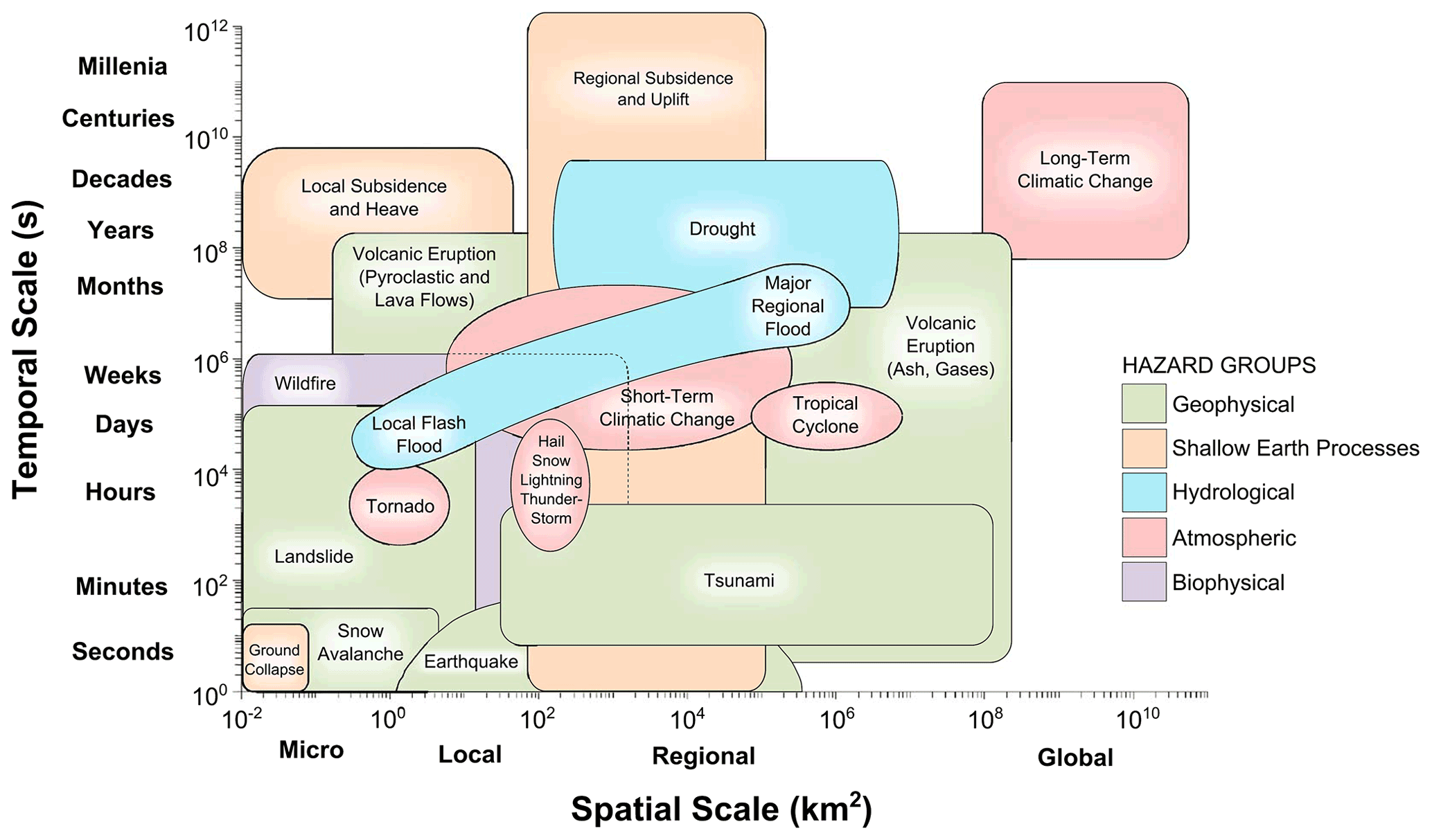
Figure 1Spatial and temporal scales of 16 natural hazards. Shown on logarithmic axes are the spatial and temporal scales over which the 16 natural hazards act. Here spatial scale refers to the area that the hazard impacts and temporal scale to the timescale on which the single hazard acts upon the natural environment. Hazards are grouped into geophysical (green), hydrological (blue), shallow Earth processes (orange), atmospheric (red), and biophysical (purple). From Gill and Malamud (2014).
Spatiotemporal clustering methods applied to environmental data can be powerful tools to understand the scales of different natural hazards by identifying natural hazard clusters (Barton et al., 2016). Such methods allow the extraction of spatiotemporal and intensity characteristics of natural hazard clusters. Estimating such characteristics is relevant when defining and understanding the potential spatial–temporal impacts of natural hazards (e.g. De Angeli et al., 2022) and their interrelation with society. Examples include the following:
-
the duration of precipitation events (Yue, 2000; Vorogushyn et al., 2010) significantly affects dike failure, landslide triggering, and flood losses;
-
the increased duration of heatwaves significantly aggravates their health impacts (Nitschke et al., 2011); and
-
the spatial extent of drought influences its impact on society (García-Herrera et al., 2019; Balch et al., 2020).
In this article, we propose a robust methodology for the spatiotemporal identification of compound hazards (SI–CH), which we use to analyse the spatiotemporal features of wind and precipitation extremes in Great Britain at various scales (from hours to days and from local to regional scale) during the period 1979–2019. This SI–CH methodology is based on spatiotemporal clustering of extreme values extracted from a gridded atmospheric dataset, the ERA5 climate reanalysis (Hersbach et al., 2019). Both extreme wind and precipitation are significant hazards in Great Britain (Pinto et al., 2012; Huntingford et al., 2014). These two hazards are usually associated with extratropical cyclones and severe storms (Zscheischler et al., 2020). Extreme wind and extreme precipitation have been defined as compound hazards (i.e. statistically dependent without causality) (Tilloy et al., 2019).
Events, including precipitation and wind extremes, have been identified as multivariate compound events (co-occurrence of multiple hazards in the same geographical region, causing an impact) (Zscheischler et al., 2020). The combination of wind and precipitation extremes can result in different and more significant impacts than the sum of the individual impacts due to extreme wind and extreme precipitation (e.g. the access to a flooded power plant due to heavy rain hindered by strong winds or road blocked by fallen trees) (Martius et al., 2016). Previous studies have quantified extreme wind and extreme precipitation co-occurrences at large scales (Raveh-Rubin and Wernli, 2015; Martius et al., 2016; Ridder et al., 2020) using climate reanalysis data, thus providing a spatiotemporal framework to study multiple variables. To detect the occurrence of extreme wind and extreme precipitation events, Raveh-Rubin and Wernli (2015) averaged wind and precipitation anomalies spatially and temporally, while Martius et al. (2016) used a threshold approach to identify extreme occurrences of wind and precipitation.
This article is organised as follows. Section 2 provides a brief background to spatiotemporal clustering. Then, in Sect. 3, the Density-Based Spatial Clustering of Applications with Noise (DBSCAN) algorithm used in the study and the gridded data retained for the analysis are introduced. This is followed by Sect. 4, wherein the SI–CH methodology steps for creating compound hazard clusters are presented, and a definition of compound hazard events in space and time is proposed. Section 5 presents the results, wherein we assess the ability of the SI–CH methodology to identify hazard events, with the resultant natural hazard clusters confronted with a set of 157 major hazard events that impacted Great Britain from 1979–2019. Spatiotemporal and intensity properties of detected single and compound hazard clusters are then analysed and discussed. Finally, in Sect. 6, we discuss the limitations of the SI–CH methodology and opportunities for its generalisation to other compound hazards.
Clustering is broadly defined as any process of grouping data by their similarities (Ansari et al., 2020) and is generally considered an unsupervised learning method because it is not guided by a priori ideas (Kassambara, 2017). It is fundamental to data analysis in various disciplines (e.g. biology, epidemiology, communication, criminology) (Xu and Tian, 2015). Clustering can be considered spatially, temporally, or the two together. In addition, two clusters of different hazards can intersect in time and space, forming a compound hazard cluster. Two hypothetical examples of spatial clustering for two hazards and their intersections to become a compound hazard event are shown in Fig. 2.

Figure 2Cartoon illustration of the footprint of two hypothetical compound hazard events over Great Britain. Hazard A (yellow) is a cluster of extreme occurrences of variable x, and Hazard B (violet) is a cluster of extreme occurrences of variable y. In (a) and (b) two hypothetical examples of spatial overlaps are shown, each a compound hazard event.
Figure 2 illustrates two compound hazard events spatially, but one can also examine compound hazard events overlapping in time and both space and time together (De Angeli et al., 2022). The significant increase in spatiotemporal data now available has created increased opportunities for spatiotemporal clustering approaches (Shi and Pun-Cheng, 2019; Ansari et al., 2020). Many methods have been developed to cluster and classify data (e.g. partition, hierarchical, density-based, model-based clustering; see for a review Milligan and Cooper, 1987; Xu and Tian, 2015). Some clustering methods have been adapted for spatiotemporal clustering (e.g. Birant and Kut, 2007; Agrawal et al., 2016; Yuan et al., 2017; Huang et al., 2019; Ansari et al., 2020). Spatiotemporal clustering is usually done with three different values characterising the data: two spatial coordinates and time (Ansari et al., 2020).
Three main approaches to spatiotemporal clustering include the following.
-
Point event clustering. This approach aims to discover groups of events close to each other in space and time. It is used, for example, to cluster seismic events in time and space (Georgoulas et al., 2013).
-
Moving clusters. This approach aims to detect behaviours of moving objects. While the identity of a moving cluster does not change over time, other attributes might change. An example is the spatiotemporal clustering of lightning strikes resulting from moving convective storms (Strauss et al., 2013).
-
Trajectory clustering. This approach captures groups of objects with similar movement behaviours, with the variable of interest being the movement itself (Yuan et al., 2017). Trajectory clustering contrasts with the moving cluster approach, wherein the moving object is of interest (vs. the movement itself). Examples of trajectory clustering include cyclone track clustering in different world regions (Ramsay et al., 2012; Rahman et al., 2018).
In spatiotemporal clustering, some approaches consider time and space as separate dimensions (e.g. Birant and Kut, 2007) with distinct clustering rules, while other approaches consider a space–time cube (e.g. Zscheischler et al., 2013; Vogel et al., 2020). In this article, we adopt a space–time cube and use the spatiotemporal ratio (Sect. 4.2.1) to control the relationship between space and time. Among other factors, the characteristics of the data used influence the choice of the spatiotemporal clustering method. Here we use climate reanalysis data, which are gridded data. Our approach aims to cluster extreme occurrences of climate variables, similarly to Kholodovsky and Liang (2021). Extreme occurrences of wind and precipitation are used to illustrate our methodology. We consider such occurrences to be point events in time and space (see Sect. 4.2) and thus select a point event clustering approach.
Spatiotemporal data include information about the location (e.g. longitude and latitude) and time of the variable of interest (Ansari et al., 2020). In this paper, we use climate data focusing on extreme wind and extreme precipitation. However, the methodology we describe here can be applied to a wide range of variables. Spatiotemporal datasets of climate variables have been derived from many different sources, including the following: observations from instrumental stations and their interpolations (e.g. E-OBS, Cornes et al., 2018), climate model outputs and reanalysis (e.g. ERA5, Hahsler et al., 2019), and remote sensing (e.g. CMORPH, Joyce et al., 2004). These have been used to analyse natural hazards and climate extremes in space and time.
To ensure spatial and temporal consistency between wind and precipitation data, we extract both of these variables from a climate reanalysis dataset. Climate reanalysis offers homogeneous datasets for numerous environmental variables, including precipitation and wind gust, with different spatial and temporal resolutions. Those data are outputs of climate models calibrated on observed data worldwide (Brönnimann et al., 2018). Two primary climate reanalysis datasets include (i) the Climate Forecast System Reanalysis (Saha et al., 2010) developed by the US National Center for Atmospheric Research (NCAR) and (ii) ERA5 (Hersbach et al., 2020) developed by the European Centre for Medium-Range Weather Forecasts (ECMWF). ERA5 (ECMWF Reanalysis 5th Generation) is used in the present study (Hersbach et al., 2018).
ERA5 was released in 2019 by ECMWF and benefits from the latest improvements in the field (Hersbach et al., 2020). The ERA5 data are available (Copernicus Climate Data Store, 2020) from 1979 to the present (we use 1979 up to September 2019), with a spatial resolution of and an hourly temporal resolution. The data resolve the atmosphere using 137 levels from the Earth's surface up to a height of 80 km (Hersbach et al., 2020). ERA5 data are generated with a short (18 h) forecast twice a day (06:00 and 18:00 UTC) and assimilated with observed data (Hersbach et al., 2020).
Reanalysis data are obtained from short-term model forecasts and can be affected by forecast errors; they are not observations (Pfahl and Wernli, 2012). Furthermore, reanalysis data offer a large amount of usable data for spatiotemporal clustering methods. The methodology described in this study could be easily extended to other atmospheric or hydrological hazards (e.g. extreme temperature, Sutanto et al., 2020). The two following variables are extracted from the ERA5 product at a spatial resolution of .
-
Extreme precipitation (p) is accumulated liquid and frozen water (mm), comprising rain and snow, that falls to the Earth's surface in 1 h (mm h−1). This value is averaged over each grid cell.
-
Extreme wind (w) is hourly maximum wind gust (m s−1) at a height of 10 m above the Earth's surface. The WMO (2022) defines a wind gust as the maximum wind speed averaged over 3 s intervals. As this duration is shorter than a model time step, this value is deduced from other parameters such as surface stress, surface friction, wind shear, and stability. This value is averaged over each grid cell.
When considering the study area boundaries, two factors should be considered: (i) the variability of climate, geology, or topography within the study area and (ii) the possibility of not capturing an event in its totality because of edge effects (Cressie, 1993). Edge effects can potentially bias clustering analyses as edge points have fewer neighbouring cells compared to other cells within the domain (Cressie, 1993). To mitigate this issue, we set a buffer area of two cells at the edge of our study area (Fig. 3). Clusters need to include extreme values (points) that are some distance away (here two cells) from the edge of the study area. A cluster of extreme values (points) exclusively within the buffer area will not be retained, but values in the buffer area can be part of other clusters. The study area chosen to illustrate the SI–CH methodology with extreme wind and precipitation contains most of Great Britain and part of northwestern France (Fig. 3). The total area of the domain is 647 900 km2 and represents a domain of approximately 1200 km (45 cells) by 500 km (33 cells), or a total of 1485 cells, with each cell (cells range from 18.6 km × 27.8 km in the south of the study region to 14.3 km × 27.8 km in the north). The temporal resolution used is 1 h over the period January 1979 to September 2019 (40 years and 9 months).
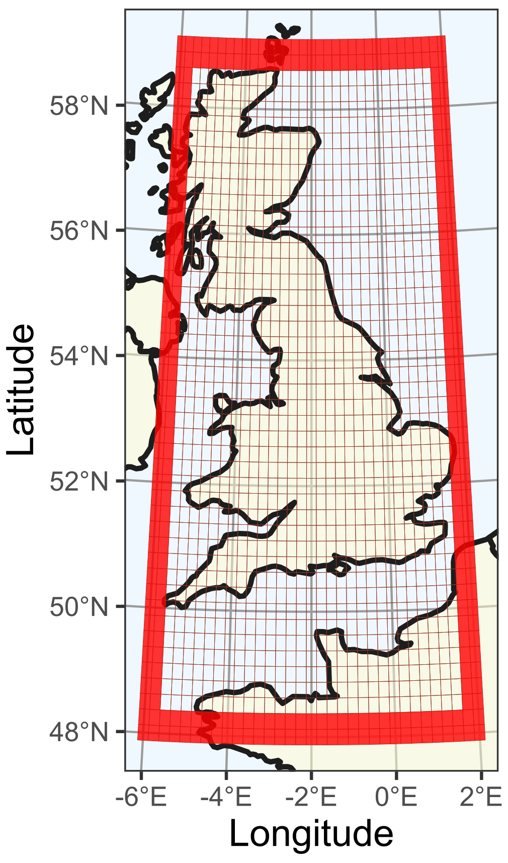
Figure 3Study area with a domain of 1485 cells (45 cells × 33 cells, each ) used for spatiotemporal clustering of extreme precipitation and extreme wind for the period January 1979 to September 2019 at 1 h time steps using ERA5 data. The area includes most of Great Britain and parts of northwestern France. The red frame is a buffer area of two cells (included in the total study area).
Both Great Britain and northern France share the same temperate oceanic climate (Koppen climate classification Cfb) (Beck et al., 2018). However, there are variations in precipitation and wind exposure within this broad region, particularly with coastal areas being more exposed to high wind and mountainous areas being wetter (Hulme and Barrow, 1997). Our methodology accounts for this variability when sampling extreme events (discussed below in Sect. 4).
Using a climate reanalysis product to study extreme events induces several limitations compared to observational data (Donat et al., 2014; Angélil et al., 2016). In climate reanalysis, variables are computed over a grid cell, and the resulting value is an average. This averaging often smooths local extreme values (Donat et al., 2014). The accuracy of reanalysis data also depends on various observation types (Hersbach et al., 2019). ERA5 benefits from the latest methodological improvements in data assimilation and modelling (Hersbach et al., 2020). Compared to its predecessor ERA-Interim, ERA5 offers finer spatial and temporal resolutions, but most importantly, it produces more accurate weather and climate data in most regions of the world (Hersbach et al., 2019; Gleixner et al., 2020; Tarek et al., 2020). Despite these improvements, the spatial resolution is still relatively coarse and small-scale convective events are still poorly captured, as is the case for most reanalysis products (Holley et al., 2014; Kendon et al., 2017; Beck et al., 2019). Furthermore, precipitation is not assimilated (calibrated on observations) in ERA5. Nevertheless, ERA5 seems to outperform other global reanalysis products for extreme precipitation (Mahto and Mishra, 2019) and captures most observed extreme precipitation events over Europe (Rivoire et al., 2021). ERA5 reproduces wind speed and wind gust more realistically compared to ERA-Interim (Minola et al., 2020). ERA5 shows good agreement with wind observations, particularly in the UK (Molina et al., 2021). However, ERA5 wind gusts can be unrealistic over high mountains and complex orography (Minola et al., 2020; Zscheischler et al., 2021).
We now discuss the methodology developed for spatiotemporal identification of compound hazard clusters. We use as an illustration wind and precipitation extremes from ERA5 reanalysis (temporal resolution 1 h, January 1979 to September 2019; spatial resolution ) over Great Britain and northwestern France. The specific clustering method used here to identify spatiotemporal clusters of extreme wind and precipitation needs to comply with two characteristics of our spatiotemporal data.
- i.
The large dataset size. ERA5 data are available for over 40 years with an hourly time step; this implies a significant amount of data over our study area of 1485 cells ( values for each variable).
- ii.
Noise level. The sample of extreme wind gusts and precipitation can produce extremes in individual and lone cells scattered in space and time, which cannot be associated with a specific hazard cluster.
We do not assume a given shape for the natural hazard clusters. This is to ensure flexibility in the specific point event clustering methodology developed. The characteristics of reanalysis climate data and the absence of assumptions about the shape of our hazard clusters guided our choice of a clustering algorithm toward the Density-Based Spatial Clustering of Applications with Noise (DBSCAN) algorithm (Ester et al., 1996; Hahsler et al., 2019). DBSCAN is a clustering algorithm for identifying clusters with arbitrary shapes (Shi and Pun-Cheng, 2019); see Supplement 1 for further details. The DBSCAN algorithm is used here as part of our overall methodology to create spatiotemporal clusters of extreme wind and extreme precipitation. The methodology to create spatiotemporal clusters is described in Fig. 4 as a flowchart of the methodology steps.
-
Variable data extraction with thresholds. Values of both variables (extreme wind, extreme precipitation) are extracted for the study area (Fig. 4). A threshold approach with a threshold u is used to sample extreme values (see Sect. 4.1).
-
Single hazard spatiotemporal clusters. The different parameters required for the clustering are set (see Sect. 4.2). Extreme values are clustered in space and time with a clustering algorithm (DBSCAN), creating two sets of clusters: (i) extreme wind and (ii) extreme precipitation.
-
Compounds hazard spatiotemporal clusters. Extreme wind and extreme precipitation clusters are paired according to their spatiotemporal overlaps (see Sect. 4.3). The footprints of compound hazard clusters in space and their duration are then identified, allowing the spatiotemporal attributes to be estimated.
The procedure's sensitivity to the different input parameters is displayed in Fig. 4 and is discussed and quantified in Supplement 2. We aim to objectively detect hazard clusters by setting the input parameters either according to physical assumptions (Sect. 4.2.1 and 4.2.2) or by following an automated procedure (Sect. 4.2.3).
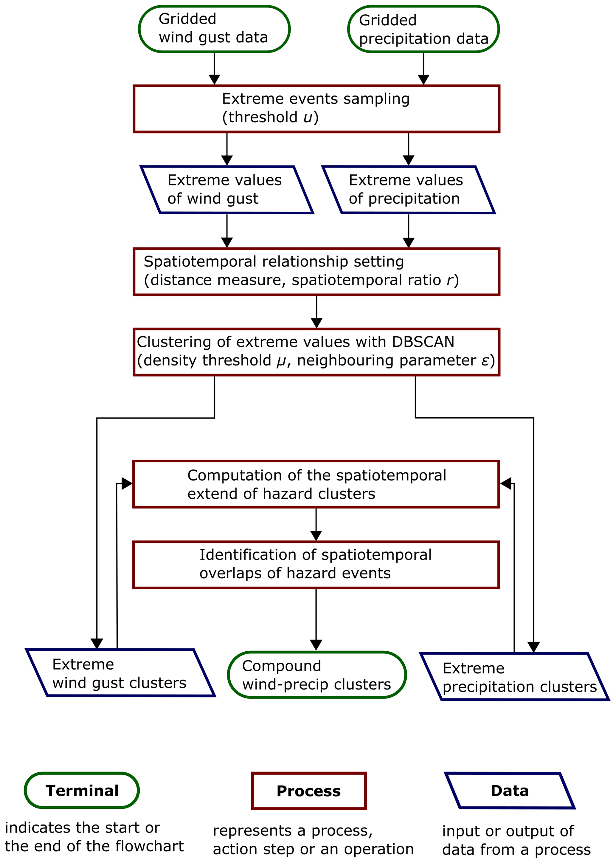
Figure 4Flowchart of the methodology developed, spatiotemporal identification of compound hazards (SI–CH), for wind and precipitation data in Great Britain. DBSCAN (Density-Based Spatial Clustering of Applications With Noise) is an integral step in our methodology to identify compound hazard clusters in time and space. The name (terminal, process, data) and function associated with the three types of symbols used in the flowchart are given at the bottom of the figure.
4.1 Defining a hazard threshold
The methodology developed here uses the occurrences of climate variables above a given threshold to represent that climate variable's extremes. These peaks over threshold serve as a proxy for the occurrence of natural hazards: in this case, extreme wind and extreme precipitation. The use of a threshold to analyse the spatiotemporal occurrence of different extremes and their potential combinations has been done with daily data by Martius et al. (2016), Sedlmeier et al. (2018), and Sutanto et al. (2020). In the latter two studies, two approaches are used to define the value of a threshold: (i) an impact-based approach whereby the threshold is related to a tipping point at which impacts start occurring (Sedlmeier et al., 2018) and (ii) a percentile-based approach whereby the threshold is related to an empirical extreme quantile of the studied variable (Tencer et al., 2014; Visser-Quinn et al., 2019; Sutanto et al., 2020). In the second approach, hazards are extreme events relative to the distribution of the studied variable.
The percentile-based approach was chosen because it provides a large sample size for robust statistical analysis. While not being linked to a specific impact, the percentile-based approach can also be impact-relevant (Zhang et al., 2011), with extreme occurrences of hourly maximum wind gusts and hourly accumulated precipitation potentially negatively impacting society. The connection between maximum wind speed and impact has been broadly acknowledged (Pinto et al., 2012). It has been shown that a local 98th percentile is an impact-relevant wind threshold (Ulbrich et al., 2009). However, as our data are not local, a 99th percentile was used to increase the probability of detecting potentially damage-relevant events. For consistency, the same percentile is used for the definition of extreme events of both hazards. The threshold is computed for each of the 1485 cells of the domain studied. The threshold values vary m s−1 for hourly maximum wind gust w and mm h−1 for precipitation p. The value of the selected percentile (here 99th) and the corresponding threshold value significantly influence the clustering procedure (Supplement 2).
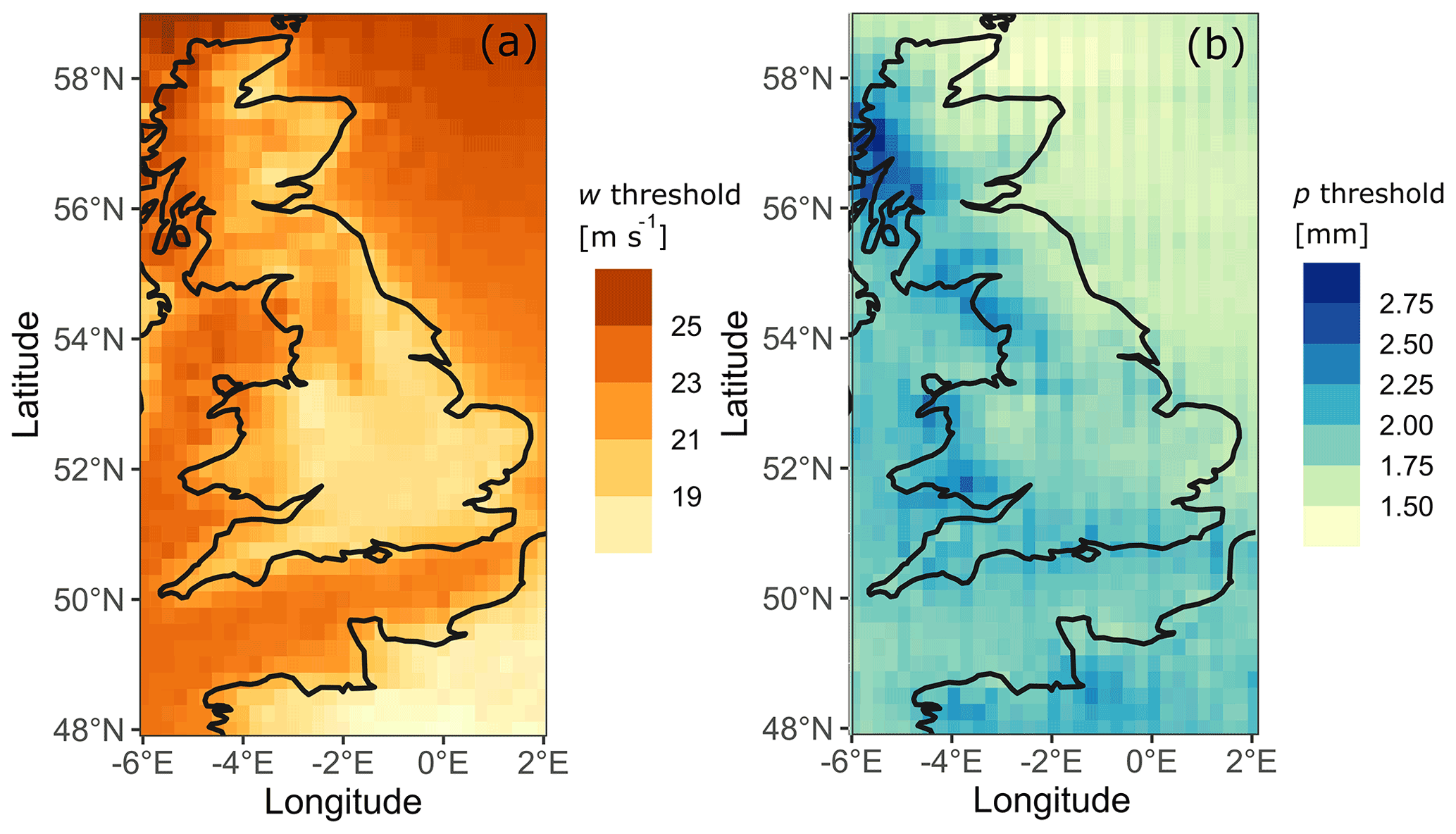
Figure 5Threshold values (see legends) used to extract extreme values for the clustering process over Great Britain and northwestern France. The values correspond to the 99th percentile on each grid cell during the period 1979–2019 for (a) hourly maximum wind gust (w) and (b) hourly precipitation accumulation (p). Data from ERA5 (Hersbach et al., 2018).
The threshold values w for wind gust and p for precipitation over the study area are displayed in Fig. 5. In this figure, the wind gust threshold is higher in coastal regions and the north of England, Scotland, and Wales. This contrasts with southern England and northwestern France, which have significantly lower threshold values. For precipitation, one can observe a clear division between the eastern and western parts of Great Britain, with the western part having significantly higher threshold values. The sample of extreme events is then composed of two distinct sets: (i) occurrences of extreme wind gusts and (ii) occurrences of extreme precipitation. These extreme events are then represented as point objects with coordinates in space (latitude and longitude) and time (date). Here, both hazards are studied separately before being paired into compound hazard events. The DBSCAN clustering algorithm is then applied to the points representing extreme wind and precipitation values.
4.2 Construction of single hazard clusters
A method for sampling extreme values has been presented in Sect. 4.1. These extreme values are the input data for the construction of the cluster. In the present study, the spatiotemporal domain is assumed to be a space–time cube as done in other studies (e.g. Bach et al., 2014). The Euclidean distance is preferred to other distance measures in our study for simplicity. One of the advantages of this approach is that it is possible to take advantage of the spatial index structure (see Supplement 1 for more details about the DBSCAN algorithm) to significantly speed up the runtime complexity (Hahsler et al., 2019). Three parameters inform the clustering procedure: (i) the relationship between spatial distance and temporal lag (r), (ii) the density threshold (μ) for our cluster, and (iii) the neighbour parameter (ε). These three parameters are now discussed.
4.2.1 First parameter: the spatiotemporal ratio r
The first step of our cluster event construction is to define the importance of spatial distance relative to temporal distance when computing the Euclidean distance between point objects. This step is done according to physical considerations. Each point object in our input data represents one occurrence of an extreme event in one grid cell. Each grid cell is 0.25∘ latitude (≃27.8 km) by 0.25∘ longitude (ranging from 14.3 km in the southern part of our study area to 18.6 km in the northern part, Fig. 2). Grid cell areas range from 397 km2 (in the south of our study area) to 517 km2 (in the north). The temporal distance between each extreme value is at least 1 h. Scaling factors are introduced to give more importance to space or time distance in a three-dimensional space–time cube (Ansari et al., 2020). We express the spatiotemporal Euclidean distance dp,q (unitless) between two point objects p and q as
with xp and xq the latitudes of the extreme value, yp and yq their longitudes, tp and tq their temporal coordinate, and a and b two scaling parameters. The ratio is the spatiotemporal parameter controlling the relationship between spatial distance and temporal lag. The scaling parameters are set to (0.25∘) = 4∘−1 and b=1 h−1, giving a ratio r=4 h ∘−1. Setting the spatiotemporal ratio to r = 4 h ∘−1 normalises the three-dimensional space–time cube (Fig. 6). A space–time cube with each point object having a spacing of 1.0 (unitless) in each dimension (longitude, latitude, time) favours the detection of continuous events in time and space without giving more importance to one dimension or the other and makes the most of the resolution of the input dataset (here ERA5). In practice, this means that a distance of 0.25∘ in space is weighted similarly to a distance of 1 h in time (Fig. 6). Nevertheless, even if each point is equally spaced in terms of longitude and latitude, this is not the case in terms of geographical distance. The sensitivity analysis performed in Supplement 2 shows that this parameter has a small influence on the number of clusters detected compared to the two other parameters of this clustering procedure.

Figure 6Space–time cube as used in the SI–CH (spatiotemporal identification of compound hazards) methodology proposed in this paper. The three small red dots represent extreme values. Each cube is for a normalised latitude × normalised longitude × normalised time period. Each side of the cube is 1.0 and unitless, with normalisation factors for latitude and longitude a (in units of ∘−1) as well as a normalisation factor for time b (h−1). Normalised latitude and longitude for our ERA5 data are (a×0.25 ∘), with a=4 ∘−1, and normalised time is (b×1 h), with b=1 h−1.
4.2.2 Second parameter: the density threshold μ
The density threshold parameter μ represents the number of neighbours a point needs to be considered a core point, thus generating a new cluster. This value needs to be greater than four points in our dataset (number of dimensions plus one) (Ester et al., 1996). However, it is not intended to detect intense small-scale events (e.g. the Bracknell storm, Berkshire, UK, on 7 May 2000) because of the relatively coarse resolution of ERA5, which tends to underestimate local precipitation extremes (Rivoire et al., 2021) and wind extremes in mountainous areas (Zscheischler et al., 2020). The aim is to detect events of varying sizes. Small-scale and short-duration extreme precipitation and/or wind events in Great Britain are often associated with convective events. Such events vary from hundreds to tens of thousands of square kilometres (Chazette et al., 2016; Rigo et al., 2019), while their duration goes from hours to days. Knowing that the area of the study area cells ranges between 400 and 520 km2, we take a density threshold μ=10 points, meaning that the minimum spatiotemporal extent of a cluster composed of at least 10 extreme values is
-
1 h over an area of 5200 km2 for a short and large cluster and
-
10 h over an area of 400 km2 for a long and localised cluster.
We refer the reader to Supplement 1 for more detailed information about core points and the sensitivity threshold.
4.2.3 Third parameter: neighbour parameter ε
This third parameter is the neighbour radius ε, in which at least μ points (here μ=10) should be included to create a cluster. In this study, the neighbourhood is a spatiotemporal domain. This parameter controls the density of extreme events required to create a cluster. An optimal value for ε depends on the dataset to be clustered and is assessed semiautomatically. The procedure to select a relevant radius for our wind and precipitation dataset is to plot the points' k–NN distances (i.e. the distance to the kth nearest neighbour) in increasing order to look for a knee in the plot. The distance to the kth nearest neighbour allows classifying data points by their similarity, here represented by their spatiotemporal distance. The idea behind this procedure is to separate points located inside clusters (with low k–NN distance) from isolated noise points (with large k–NN distance) (Hahsler et al., 2019). Here . More details about this step are available in Supplement 1.
4.2.4 Single hazard cluster parameters summary
The three parameters of the clustering procedure (r, μ, ε) are now set. The spatiotemporal space has been discretised in a space–time cube (Fig. 6). Each grid point (representing one grid cell of input data) is spaced by a unit distance in each direction (longitude, latitude, time). A unit distance represents 0.25∘ in the spatial dimension and 1 h in time. The density threshold (μ) has been fixed at μ=10 points. A k nearest neighbour (k–NN) search was performed with points. The result is a distance matrix containing the distance of each point to its 10–NN, allowing us to fix the neighbour parameter at ε=2.24 for extreme wind and ε=2.45 for extreme precipitation values. This information makes it possible to estimate the spatiotemporal domain in which the 10–NN needs to create a new cluster. This 10–NN neighbourhood includes nmax=44 points (see Fig. S1.3) with a maximum temporal distance of 2.0 h and a maximum spatial distance of 0.5∘ in latitude or longitude. The sensitivity of the clustering procedure to (r, μ, ε) is assessed in Supplement 2.
4.3 Compound hazard events
One commonly used option to study compound extremes is to sample only the joint extreme events (i.e. extreme wind and extreme precipitation at a given location and time) (Martius et al., 2016; Tencer et al., 2016; Sutanto et al., 2020; Zhang et al., 2021). However, when detecting the spatial and temporal characteristics of compound extremes, this option has the following weaknesses: (i) a high reliance on the spatial and temporal resolution of the input data in the definition of compound, (ii) lack of considering the lag time between different extremes, and (iii) difficulty deciphering the spatial structure of extreme events. Our approach aims to overcome these weaknesses.
Here, single hazard event clusters are created for both extreme wind and extreme precipitation. Compound hazard events are then detected by spotting the overlap of the extreme wind and extreme precipitation events in time and space. The footprint of a compound hazard event is the total area impacted for a duration of time. To define a compound hazard event's spatial and temporal scales, one can look at the overlap in time (t) and space (S) of single hazard event clusters. This overlap can be the intersection AND (tw∩r, Sw∩r) or the union OR (tw∪r, Sw∪r) of the two hazard events in space and time. There are therefore four different possible definitions of a compound hazard event in space and time depending on the definition chosen for the overlap in space and time, as displayed in Fig. 7. The extent of the compound hazard event footprint widely varies depending on which combination of spatial and temporal overlap is retained. One can consider the following.
- a.
The duration of a compound hazard event can either be defined as the time during which both hazards occur (AND) or as the aggregated duration of both hazards (OR). As the potential impact caused by a hazard can remain after the occurrence of this hazard (e.g. fallen trees blocking a road), the temporal scale of a compound hazard is then defined as the aggregated duration (tw∪r) of both single hazard events.
- b.
Footprints from different hazards need to overlap at least at one point to create a compound hazard event. The spatial scale of compound hazards is defined here as the intersection (Sw∩r) of the footprint of the two single hazards.
An overlap of the two hazards' footprints does not mean that the two hazards occur in the overlapping area at the same time (here same hour) but that the two hazards occurred, during at least 1 h each, in that area during the same compound hazard event. This approach overcomes the weaknesses as mentioned above of constructing a joint occurrence sampling method without introducing a lag time (Klerk et al., 2015; Iordanidou et al., 2016). The time window in which a compound event can occur is flexible and fixed by the duration of both hazard events.

Figure 7Different spatial and temporal scales considered in this study to define compound hazard events, with each case representing a combination of spatial and temporal overlap. Panel (a) shows [spatial AND] with [temporal OR], (b) [spatial AND] with [temporal AND], (c) [spatial OR] with [temporal OR], and (d) [spatial OR] with [temporal AND]. Hazard A is orange, hazard B is in purple, compound hazard is in blue, and parts of the footprints outside the temporal boundaries are grey. The definition retained for the rest of the study is highlighted with a red frame (a).
We define the compound hazard event footprint (Fig. 6a) here as the intersecting area (AND) on which two (or more) hazards develop during the aggregated union of the time periods (OR) of the two hazard events. We believe this definition is the most relevant in terms of impacts as it accounts for potential cascading or compounding impacts in time and space of two (or more) hazards (e.g. flooding of a building caused by a destroyed roof and heavy precipitation). From this definition and the illustration in Fig. 6a, the spatial (S) and temporal (t) scales of a compound (“Comp”) hazard event that includes wind (w) and precipitation (p) events are defined as follows:
with t the duration and S the area of the compound hazard event (tComp, SComp), wind event (tw, Sw), and precipitation event (tr, Sr). The duration of a compound hazard event corresponds to the union of the durations of both hazard events involved, meaning that . This paper examines compound wind–precipitation events; however, this definition applies to other compound hazards (e.g. extremely hot temperature and drought).
Table 1Intensity and spatiotemporal attributes of hazard clusters and their availability for wind, precipitation, and compound hazard events in the present study.
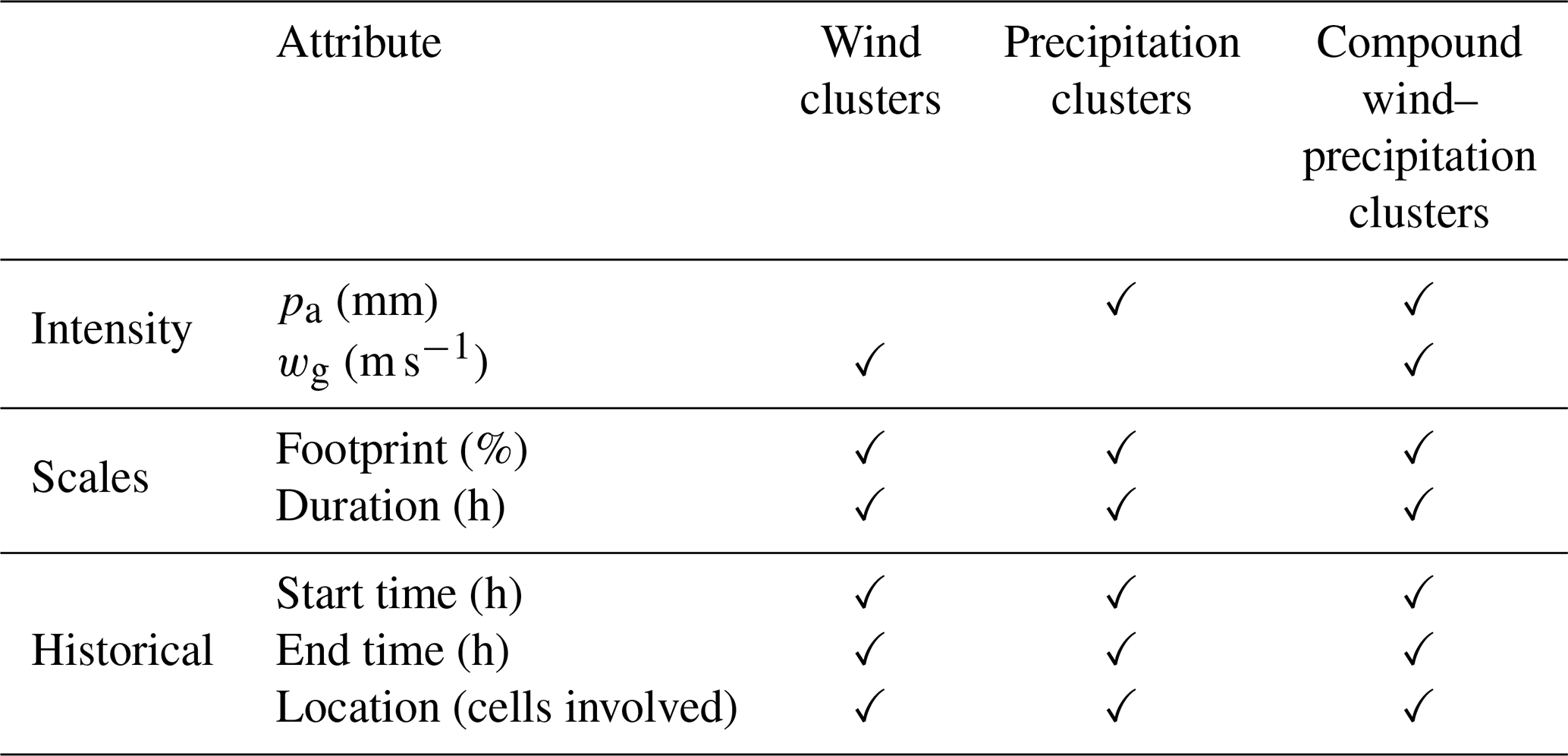
4.4 Single and compound hazard cluster attributes
In our SI–CH methodology, each single and compound hazard cluster created is characterised by a set of attributes. Similarly to Visser-Quinn et al. (2019), three attributes (or metrics) are developed here: (i) intensity attributes, (ii) spatiotemporal attributes, and (iii) historical attributes as follows.
- i.
Intensity attributes for each variable
- a.
Maximum precipitation accumulation (pa). To represent the intensity and magnitude of precipitation in a given grid cell, the accumulated precipitation in millimetres (pa) over the total duration of a cluster is used. Here, precipitation accumulation represents the total amount of precipitation accumulated over the duration of a cluster over one grid cell, including time steps when the precipitation value is below the 99th percentile threshold. To retain a single value characterising a cluster, the largest value of pa among all the grid cells included in a cluster is retained.
- b.
Peak wind gust (wg). The peak wind gust is the maximum wind gust over a grid cell over the duration of a cluster. The maximum peak wind gust expresses the intensity of a wind cluster in the cluster duration in metres per second (m s−1).
Intensity attributes for both precipitation and wind gust, as given above, represent a local maximum within clusters and not an average or a sum over the cluster footprint.
- a.
- ii.
Spatiotemporal attributes
- a.
The spatial extent is measured in grid cells (). It represents the total number of grid cells (Fig. 2) involved in the cluster.
- b.
The temporal extent (or duration) is measured in hours. The temporal extent represents the difference between the last and first time step in which the cluster occurs.
- a.
- iii.
Historical attributes include the following:
- a.
the start and end date of an event;
- b.
the season of
-
December–January–February (DJF),
-
March–April–May (MAM),
-
June–July–August (JJA), or
-
September–October–November (SON); and
-
- c.
the location, meaning the grid cells involved in the cluster.
These attributes are summarised in Table 1.
- a.
This section presents the results of applying our SI–CH methodology to ERA5 precipitation and wind variables for 1979 to 2019 in the UK. From these attributes (Table 1), the distribution of scales attributes is presented and discussed along with other characteristics of the wind, precipitation, and compound hazard database created (Sect. 5.1). Historical attributes of the hazard clusters created are confronted with a catalogue of 157 observed significant Great Britain weather events. This confrontation highlights our methodology's capabilities and the ability of the ERA5 reanalysis to detect different types of extreme events in Great Britain (Sect. 5.2). The scales and intensity attributes of detected clusters are then analysed with examples from the significant events catalogue (Sect. 5.3).
5.1 Wind, precipitation, and compound clusters identified using the SI–CH methodology
We apply the SI–CH methodology (Sect. 4) to the spatiotemporal dataset presented in Sect. 3 for January 1979 to September 2019 and detect 18 086 precipitation clusters, 6190 wind clusters, and 4555 compound hazard clusters. The detailed attributes for these single and compound hazard clusters are given in the ERA5 Hazard Clusters Database 1979–2019 (Supplement 3), including the attributes in Table 1.

Figure 8Footprints of 10 example natural hazard clusters from the ERA5 Hazard Cluster Database (Supplement 3): three precipitation clusters (a–c), three wind clusters (d–f), and four compound hazard clusters (g–i) detected by the SI–CH methodology proposed in this paper. The cluster ID (P = precipitation, W = wind, C = compound) is given at the top of each graph. The compound clusters shown include one P and one W cluster: (g) C233=P1162 and W387; (h) C141=PR766 and W220; (i) C2600=P10 041 and W3717; (i) C2601=P10 042 and W3717. W3717 is shared by both compound clusters C2600 and C2601. Clusters with areas that are small (footprint < 9 cells) are shown in the left column (a, d, g), medium (19 cells < footprint < 32 cells) in the middle column (b, e, h), and large (footprint > 316 cells) in the right column (c, f, i). The definition of small, medium, and large for single and compound hazard clusters is derived from the quantiles of the footprint distributions (q10, q50, q95). Circle size represents the duration of single or compound hazard clusters in each cell.
A total of 10 examples of clusters of various sizes and durations detected by the SI–CH methodology are displayed in Fig. 8. For each type of cluster (precipitation, wind, compound), the footprints of one small, one medium, and one large cluster are presented. These examples illustrate the diversity of shape, area, and duration of wind and precipitation clusters detected. For compound hazard clusters (Fig. 8g–i), different configurations are displayed: a small compound hazard cluster at the intersection of two large precipitation and wind clusters (Fig. 8g), a small precipitation cluster contained within a large wind cluster (Fig. 8h), and a large wind cluster associated with two precipitation clusters (Fig. 8), creating two distinct compound hazard clusters.
In our SI–CH methodology, we decided to have each compound cluster comprised of just two clusters: one precipitation and one wind cluster. Therefore, an extreme precipitation (or wind) cluster with the same ID can be part of two (or more) different compound hazard clusters, as displayed in Fig. 8i. These compound clusters might overlap in time and/or space. The 4555 compound hazard clusters we detected consist of 3565 precipitation clusters with a unique ID (20 % of the 18 086 single hazard precipitation clusters) and 2913 wind clusters with a unique ID (47 % of the 6190 single hazard wind clusters). For example, an extratropical cyclone bringing extreme precipitation scattered in space and time could be identified as several compound hazard clusters composed of different precipitation clusters and one single extreme wind cluster. In our database of 4555 compound hazard clusters, we found the following distribution of unique single event hazard cluster IDs.
-
Of the 3565 precipitation clusters with a unique ID, 2912 (82 %) are each found in one unique compound cluster, 578 (16 %) in two to three different compound clusters, and 75 (2 %) in four to nine different compound clusters.
-
Of the 2913 wind clusters with a unique ID, 2053 (70 %) are found in one unique compound cluster, 663 (23 %) in two to three different compound clusters, 156 (5 %) in four to five different compound clusters, and 41 (1 %) in 6–14 different compound clusters.
Regarding the distribution of exclusive vs. non-exclusive single hazard clusters making up the compound clusters, where exclusive means a unique single hazard ID (wind or precipitation) is found in only one compound hazard ID, we found the following.
-
Non-exclusive wind ID and non-exclusive precipitation ID clusters: 559 (12 %) compound clusters.
-
Non-exclusive wind ID and exclusive precipitation ID clusters: 1943 (43 %) compound clusters.
-
Exclusive wind ID and non-exclusive precipitation ID clusters: 1084 (24 %) compound clusters.
-
Exclusive wind ID and exclusive precipitation ID clusters: 969 (2 %) compound clusters.
Figure 9 presents the probability distributions of duration (h) and footprint (% of the study area) for the 4555 compound, 18 086 precipitation, and 6190 wind clusters. The diamond for each violin plot represents the average of the values for the given variable. Precipitation, wind, and compound clusters vary in shape, size, and duration. In Fig. 9a, we observe that for the footprint, wind clusters (9.0 %) are on average larger than precipitation (5.0 %) and compound clusters (4.6 %). Footprints range from one grid cell, representing <0.1 % of the study area, to 100 % of the study area for wind and precipitation clusters and 89 % for compound hazard clusters. The duration (Fig. 9b) of single and compound hazard clusters varies from 1 h to 4 d, with compound clusters lasting on average 24 h, which is much longer than wind (average 9.6 h) and precipitation (average 6.8 h) clusters. Only 2.4 % of precipitation clusters have a duration longer than 24 h compared to 8.8 % of wind clusters and 43.5 % of compound hazard clusters. The long duration of compound hazard clusters can be explained by the definition of compound hazard events presented in Sect. 4.3. Figure 9 highlights the capacities of our approach to adapt to different input data.
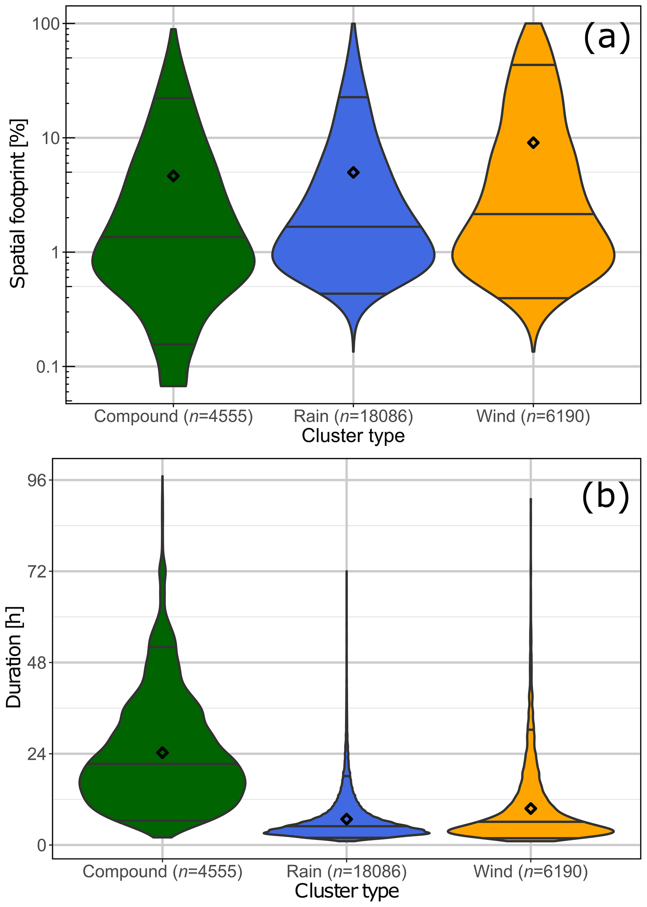
Figure 9Violin plots for 4555 compound, 18 086 precipitation, and 6190 wind clusters for January 1979 to September 2019 from the ERA5 Hazard Clusters Database 1979–2019 (Supplement 3). Shown are (a) the spatial scale as a percentage of the total study area and (b) duration in hours (h). Black diamonds represent the mean of the distributions. Quantiles 0.05, 0.5, and 0.95 are also displayed with horizontal lines. See Fig. 8 for 10 examples of clusters.
5.2 Event identification: confrontation with significant events
To assess the capacity of our methodology to identify observed hazard events, natural hazard clusters from the ERA5 Hazard Cluster Database (Supplement 3) are confronted with a set of past significant hazard events that impacted Great Britain. To do so, we created a Great Britain Significant Weather Events Catalogue 1979–2019 (Supplement 4) consisting of 157 significant Great Britain weather events between January 1979 and September 2019. The 157 significant events selected aim to represent a broad range of events, including extreme precipitation and/or extreme wind impacting Great Britain. The construction of the catalogue is done using four primary sources.
-
The British Weather Disasters (1901–2008) (Eden, 2008) is a chronology of severe weather events in the UK.
-
The Global Active Archive of Large Flood Events (1985–present) (Brakenridge, 2021) is an archive of flood events derived from news, governmental, instrumental, and remote sensing sources.
-
The EM-DAT (Emergency Events Database) (1984–2020) (CRED, 2020) is a record of disasters maintained by the Centre for Research on the Epidemiology of Disasters (CRED).
-
The past weather events website (1990–2020) (Met Office, 2020) is an archive of reports on past weather events from the UK Met Office.
These sources do not focus exclusively on extreme precipitation and wind events. Therefore, creating our significant Great Britain weather events catalogue involves a pre-selection based on the event's relevance to the study. We used the following criteria for inclusion in our catalogue.
-
An event must include extreme precipitation and/or extreme wind (the source mentions that it is extreme, which is often relative to the source and/or location).
-
The event duration must not exceed 5 d (which is above the maximum duration of clusters detected by the SI–CH method, see e.g. Fig. 8b). For example, this removed events which were “extreme precipitation/flood” events recorded as occurring over weeks or months, for which the source did not separate precipitation duration and flooding duration. For these, the same event with the duration of the extreme precipitation event was found from another source and included (as they were usually ≤5 d). Overall, <10 % of “extreme” events were removed for having a time duration > 5 d.
-
When multiple sources identified the same event, the authors judged which source had the most accurate representation of that event.
Most of the extreme events, according to the sources, were selected, with an emphasis on events recorded in more than one source. Particular attention was given to selecting events of various sizes and durations. The four sources are used to identify each event's timing, location, and duration. Duration is expressed in days, while each event's location corresponds to the 11 NUTS1 regions of Great Britain (ONS, 2021): Northeast (England), Northwest (England), Yorkshire and the Humber, East Midlands (England), West Midlands (England), East of England, London, Southeast (England), Southwest (England), Wales, and Scotland. An event can occur over one or more NUTS1 regions. Their dominant hazards are also characterised by significant events (the primary hazard reported in the sources).
Events per year for 1979–2019 are divided into precipitation events (P) and wind events (W), depending on their dominant hazard as given in the four databases above (Eden, 2008; CRED, 2020; Met Office, 2020; Brakenridge, 2021). Some significant events also include associated hazards (e.g. landslides) when reported by the sources. We use these sources to compile a significant Great Britain weather events catalogue for 1979 to 2019, which contains 96 extreme precipitation events (P) and 61 extreme wind events (W) and is given in its entirety in Supplement 4. Figure 10 shows the date and region of occurrences of the 157 significant events in our catalogue: 96 extreme precipitation events (heavyweight blue circles) and 61 extreme wind events (heavyweight orange crosses). Of the 157 events in the significant weather events catalogue, 24 can be considered compound hazard events (lightweight green circle overlain by a cross) in which extreme wind and extreme precipitation are both reported in Supplement 4. As mentioned previously, events can occur in one or more NUTS1 regions. Of the 157 catalogue events, 63 (40 %) are in one NUTS1 region, 29 (18 %) in two NUTS1 regions, 23 (15 %) in three NUTS1 regions, 18 (11 %) in four to six NUTS1 regions, and 24 (15 %) in 10 to 11 NUTS1 regions. The latter are events covering the majority of Great Britain.
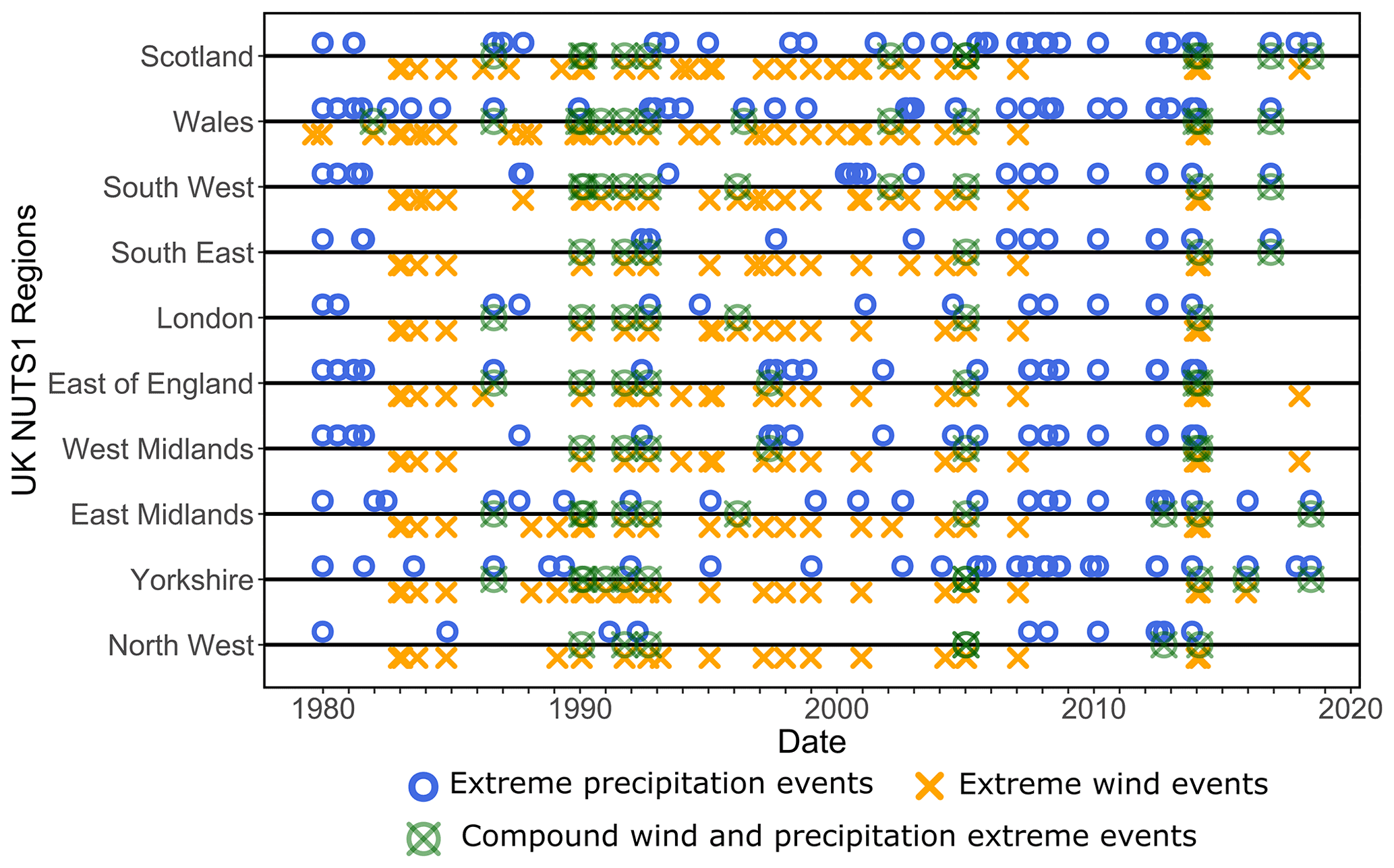
Figure 10Timeline of 157 events in our Great Britain Significant Weather Events Catalogue 1979–2019 (Supplement 4) used to assess the detection abilities of the SI–CH methodology for the 11 NUTS1 regions of Great Britain. Significant events are considered to be precipitation (96 events, heavyweight blue circles) or wind (61 events, heavyweight orange crosses). Of the 157 events in the significant weather events catalogue (Supplement 4), 24 can be considered compound hazard events (lightweight green circle overlain by a cross) as given in the sources.
In Fig. 10, we observe the interconnections between regions impacted by the same events (e.g. January 2010 precipitation event) and the clustering of events in time. Some regions are also more represented than others in our catalogue. The number of events per region is displayed in Fig. 11a, with Southwest England and Wales being the regions with the most events and Northeast England and the East of England being the regions with the fewest events.
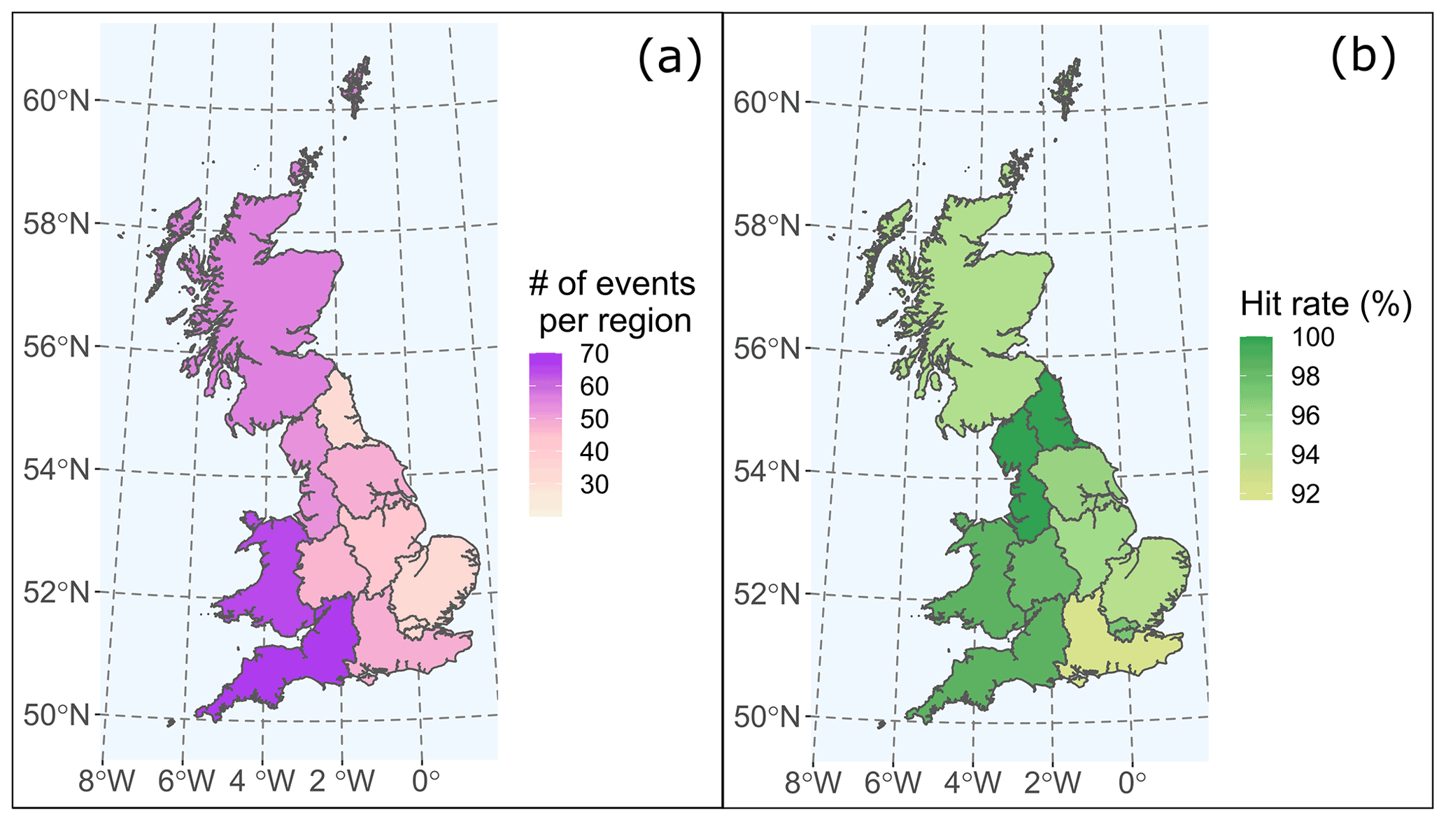
Figure 11Map of Great Britain divided into 11 NUTS1 regions showing (a) the number of events per region from our Great Britain Significant Weather Events Catalogue 1979–2019 (Supplement 4) and, (b) for each region, the hit rate (ratio between the number of joint events and the total number of events in our significant weather events catalogue).
The date and locations of the 157 events are then used to assess our clustering method's ability to capture extreme wind or extreme precipitation events. For each event in our Great Britain Significant Weather Events Catalogue 1979–2019 (Supplement 4), a temporal and spatial match is performed to identify the corresponding cluster(s) in our ERA5-based variable results from Sect. 5.1. There are 11 NUTS1 regions. For a spatiotemporal match to occur, the following needs to be true.
-
A cluster needs to occur in the same NUTS1 region(s) as the significant weather event catalogue event.
-
A cluster needs to occur during the same day(s) as a significant weather event from the catalogue (Supplement 4).
The hit rate (ratio between the number of events with corresponding clusters and the total number of events) is used to assess the capacity of the SI–CH methodology. Over Great Britain, 147 out of 157 (hit rate 93.4 %) significant events have one or more corresponding hazard cluster(s) when spatial and temporal matching is done. The hit rate is slightly higher for the subgroup of extreme wind events (95.1 %) than for extreme precipitation events (92.6 %). Among these 147 events, 64 (43.5 %) have exactly one corresponding cluster. The percentage of detected events for each NUTS1 region varies between 91.7 % (Southeast England) and 100 % (Northwest England, Northeast England) and is displayed in Fig. 10b. Among the 147 events with clusters associated, 109 are identified as compound hazard events by the SI–CH method ( for compound hazard events reported in the weather events catalogue). More than 4 times more compound hazard events are identified by the SI–CH method compared to the catalogue, suggesting that compound hazard events are underreported in our catalogue (Supplement 4).
A total of 10 of 157 events present in our Great Britain weather events catalogue but not detected by the DBSCAN algorithm are heterogeneous with no clear seasonal pattern. Among these 10 events, 6 have temporally corresponding clusters, with clusters occurring the same day as those detected by the algorithm but occurring in other NUTS1 regions. The 10 events are small- or medium-scale (8 of the 10 reported events occur in one or two NUTS1 regions), and 7 out of 10 events are extreme precipitation. The absence of clusters associated with some events means that there is not a sufficient number of extreme values of wind–precipitation in the NUTS1 region where the significant event occurs to trigger the creation of a cluster in that area. This could be due to the high value of the threshold for extreme values (u=0.99). Another explanation is that ERA5 could not reproduce these events, as the dataset can miss localised extremes, particularly for precipitation (see Sect. 3).
5.3 Spatiotemporal properties of compound wind and precipitation extremes in Great Britain
Only a minority of the single and compound hazard clusters detected during 1979–2019 can be associated with events that led to considerable damage (e.g. Great Storm of 1987, Storm Xaver). We now illustrate the SI–CH methodology using three examples from the significant events catalogue. Spatiotemporal properties of single and compound hazard clusters in relation to hazard intensity are then discussed.
The intensity of precipitation and wind events is assessed with the intensity attributes presented in Table 1. Values of precipitation accumulation and peak wind gust are subject to uncertainties (Sect. 3). Therefore, precipitation accumulation and wind gust duration values are transformed onto the standard uniform space on the interval [0, 1]. The empirical cumulative probability expresses the intensity of hazards for both wind peak and precipitation accumulation as follows:
where Rx,i represents the rank of observation xi in the sorted values of pa or w (i=1 for the smallest observation, i=N for the largest), and Nx is the sample size (here the total number of values over the period of study). For compound hazard clusters, the combined intensity is expressed by the minimum cumulative probability of the two hazards:
where Rx,i (Ry,i) represents the rank of observation xi (yi) in the sorted values of pa (w) (i=1 for the smallest observation, i=N for the largest), and Nx (Ny) is the sample size.
Figure 12 highlights the footprint of three hazard clusters and the intensity field of single and compound hazards within the clusters. Figure 12a shows the footprint of a precipitation cluster that occurred in July 2007 (Supplement 3, ERA5 Hazard Clusters Database 1979–2019, P12593). The total footprint occupies the vast majority of Wales and southern England. However, the most intense precipitation values are confined to the West Midlands, where most flooding and impacts were reported (Eden, 2008). Figure 12b shows the footprint associated with Storm Xaver (December 2013), which develops over 73 % of the study area with varying intensity (Supplement 3, ERA5 Hazard Clusters Database 1979–2019, W5423). The most extreme winds occurred in Northeast England, Scotland, and the North Sea. Figure 12c highlights the compound hazard footprint of the cluster associated with Storm Angus (November 2016), with extreme precipitation and wind combining at high intensities, mainly over the British Channel (Supplement 3, ERA5 Hazard Clusters Database 1979–2019, C4172).

Figure 12Footprint and intensity of precipitation and wind clusters (from the ERA5 Hazard Clusters Database 1979–2019, Supplement 3) associated with three significant events from our Great Britain Significant Weather Events Catalogue 1979–2019 (Supplement 4). The footprint as a function of intensity for all pixels for each of these three events is given: (a) Catalogue Event 130, extreme precipitation (Hazard Cluster Database P12593); (b) Catalogue Event 146, extreme wind, associated with Storm Xaver (Hazard Cluster Database W5423); (c) Catalogue Event 154, compound wind and precipitation event associated with Storm Angus (Hazard Cluster Database C4172).
Figure 13 features spatial–quantile plots displaying the footprint as a percentage of the study area in Fig. 3 of clusters as a function of their intensity. The more the curve goes toward the top right corner of the plot, the more severe the cluster is (high intensity over a large footprint). The footprint is expressed as the number of cells which have a varying spatial area depending on the latitude (see Sect. 3), with cell areas in our study region varying from 398 km2 (in the north) to 517 km2 (in the south), a change of approximately 30 %. An intensity of I=0.00 represents the minimum intensity value in our sample of extremes (1.42 mm for precipitation over the duration of the event over all event cells and 17.11 m s−1 for wind over a given cell for all events). Clusters related to events in the catalogue are highlighted in colours, while other events are grey. The three clusters displayed in Fig. 12 are in dark blue in Fig. 13 for (a) precipitation, (b) wind, and (c) compound wind and precipitation extreme clusters. It is important to note that compound hazard clusters in Fig. 13c are constructed with single hazard clusters from (a) and (b). In Fig. 13, each curve corresponds to a cluster and shows the evolution of the footprint (number of cells) as a function of their intensity. For example, cluster P12593 has a total footprint of approximately 28 % of the study area with an intensity (I) above 1.42 mm; this footprint drops to 25 % for an intensity above q50 (9.99 mm) and 4 % for an intensity above q99 (40.14 mm). The colour of each curve represents the total duration of each cluster.

Figure 13Spatial–quantile plot for 18 086 precipitation, 6190 wind, and 4555 compound clusters for January 1979 to September 2019 from the ERA5 Hazard Clusters Database 1979–2019 (Supplement 3). The footprint (in percent of the total area) is given as a function of the intensity of single and compound hazard events. The intensity (from 0.00 to 1.00) is expressed by (a) the cumulative probability (Eq. 3) of the precipitation accumulation at each grid cell during all precipitation events, (b) the cumulative probability (Eq. 3) of the wind “accumulation” at each grid cell during all wind events, and (c) the minimum cumulative probability (Eq. 4) of the compound hazard (wind + precipitation) events. Coloured curves represent clusters associated with events from our Great Britain Significant Weather Events Catalogue 1979–2019 (Supplement 4); colours represent the duration of the events. Grey lines represent all other events in each database (Supplement 3). The blue curve in each part represents the individual hazard event clusters for precipitation, wind, and compound displayed in Fig. 12. In panel (a), the green curves represent the clusters matched with unique event 62 from our Great Britain Weather Events Catalogue.
From Fig. 13, we also observe that the largest (highest footprint at intensity 0.0) and most intense (highest footprint at intensity 1.0) clusters are primarily associated with the 157 significant events presented in Sect. 5.2. This suggests that events from the catalogue developed in Sect. 5.2 correspond to the most noteworthy clusters obtained from the SI–CH methodology. However, several clusters have a short duration, small footprint, and moderate intensity associated with the 157 significant events, particularly for precipitation clusters (Fig. 13a). This is because more than one cluster can have a spatiotemporal match with a significant event from the catalogue. A significant precipitation event from the catalogue has a spatiotemporal match with on average 2.8 precipitation clusters. A wind event from the catalogue matches on average 1.6 wind clusters. A compound hazard event from the catalogue matches on average 2.1 compound clusters. In practice, a significant event can be associated with one large and/or intense cluster and several small clusters. This is particularly true for events that have a long duration recorded in the catalogue, such as event 62, which is associated with one large and intense precipitation cluster (P6058) and several small and low-intensity precipitation clusters (P6047; P6048; P6049; P6054, and 6055). These clusters are displayed in dark green in Fig. 13a.
Assessing the characteristics of compound hazard events in space and time brings valuable insight into the nature of the relationship between the hazards involved in the event. It overcomes the main limitations of compound hazard studies which focus on interrelations at specific sites (Sadegh et al., 2018). However, spatiotemporal analysis of compound hazards brings its own set of uncertainties and limitations. This section will discuss the following five main limitations arising from the presented study:
-
parameters influencing the clustering procedure,
-
the subjective definition of compound hazard events in space and time,
-
biases and uncertainties around the estimation of attributes,
-
influence of the method and the input data on the results, and
-
additional exploration of the spatiotemporal features of compound wind–precipitation clusters in the ERA5 Hazard Clusters Database 1979–2019.
Parameters influencing the clustering procedure. Three main parameters influence the clustering process and consequent results; their influence is discussed further and quantified in Supplement 2.
- i.
The first parameter is the threshold (u) selected to sample extreme events. This study is based on the assumption that an extreme enough occurrence of an environmental variable can be used as a proxy for natural hazard identification. A threshold is then set to sample the extreme occurrences of environmental variables. Even if this threshold has been selected in light of previous works on wind and precipitation extremes (Ulbrich et al., 2009; Martius et al., 2016), its value remains subjective. A seasonal threshold could also have been used to detect more events during the extended summer. The threshold value directly impacts the number of extreme events sampled and therefore the selection of the other clustering parameters (Supplement 2).
- ii.
The second parameter is the ratio r of the spatiotemporal scaling parameters a and b. A three-dimensional Euclidean distance is used as a distance measure for the clustering procedure. The value of the distance between each extreme event is controlled by the importance given to the spatial (longitude and latitude) and temporal (time) component in the input data. For simplicity, each component was set to have the same importance in the distance computation, meaning that more importance could be given to the time (or space) component depending on a prior assumption (Zscheischler et al., 2013; Vogel et al., 2020).
- iii.
The third parameter is density threshold μ. While the neighbouring parameter ε is set systematically (Sect. 4.2), its value depends on the density threshold, giving the minimum number of detected events per cluster. The selection of μ is based on a prior assumption about the minimum size a compound hazard event can have in the context of the study.
The subjective definition of compound hazards events in space and time. Section 4.3 presented four possible definitions for a compound hazard event in time and space. It was chosen to define the duration as the aggregated duration of all hazard clusters. However, one could be more interested in extracting the simultaneous duration of both hazards or considering the total area impacted by the two hazards (Zscheischler et al., 2020).
Biases and uncertainties around the estimation of attributes. There are biases and uncertainties around the values of intensity attributes of the events. These biases are partly due to the data used in this study: the ERA5 reanalysis data (Sect. 2). Higher uncertainty arises from precipitation accumulation estimation as precipitation observations are not assimilated in ERA5. Biases might also be more pronounced over mountainous areas (Skok et al., 2016; Sharifi et al., 2019), which are more exposed to compound wind and precipitation events (see Appendix A and below). The size of the study area also leads to some events being detected only partially, which could bias our estimates of the size and duration of events.
Influence of the method and the input data on the results. The method's performance developed here is assessed using a catalogue of major events built using different observational datasets that are not related to ERA5. This approach makes disentangling the influence of the clustering method (SI–CH) and the data (ERA5) difficult. A way to identify the source of the performance would be to apply the clustering method to a different dataset, ideally observational (e.g. CMORPH for precipitation). Additionally, the hit rate observed in this study for extreme precipitation is higher than the one obtained by Rivoire et al. (2021). This suggests that the clustering method used in the present study improves the ability to identify extreme events with ERA5. However, differences in spatial and temporal resolution of the extremes and the reference dataset complicate the comparison between the two studies.
Additional exploration of the spatiotemporal features of compound wind–precipitation clusters in the ERA5 Hazard Clusters Database 1979–2019 (Supplement 3). The ERA5 Hazard Clusters Database 1979–2019 that we have produced in this paper can also be exploited for a number of other spatial–temporal attributes. In Appendix A we explore some of these, including the following:
-
the proportion of compound hazard clusters among wind and precipitation clusters with respect to
- a.
the size and duration of these clusters (Fig. A1) and
- b.
their location (Fig. A2);
- a.
-
the frequency of occurrence of compound wind–precipitation events over Great Britain, allowing the identification of compound wind–precipitation hotspots (Fig. A3);
-
the strength of the spatiotemporal dependence between precipitation clusters and wind clusters using the likelihood multiplication factor (LMF) (Fig. A3);
-
the seasonality of wind, precipitation, and compound hazard clusters (Fig. A4);
-
the monthly frequency of compound hazard clusters amongst the total number of clusters (Fig. A5); and
-
the spatial dependence between different sites (Fig. A6).
The SI–CH methodology described in this paper has produced our ERA5 Hazard Clusters Database 1979–2019 (Supplement 3), which has a richness of information which can be exploited to better understand the spatial–temporal characteristics of these compound events. Appendix A shows some of these potential characteristics which can be explored. The link between compound wind and precipitation extremes and weather systems is discussed in Appendix A; nevertheless, this link could be explored in greater depth with quantitative approaches similar to Catto and Dowdy (2021), who examine compound hazards from a weather system perspective.
To characterise compound hazard events of extreme precipitation and extreme wind in Great Britain more accurately, their overlap in space and time has been analysed. By clustering extreme occurrences of maximum hourly wind gust and hourly precipitation from ERA5, 4555 compound wind–precipitation clusters over Great Britain were identified for 1979–2019 (ERA5 Hazard Clusters Database 1979–2019, Supplement 3). To assess the ability of the approach to identify the occurrence of extreme events in time and space, we identified 157 extreme precipitation and/or extreme wind events that occurred in Great Britain over the period 1979–2019 (Significant Great Britain Weather Events Catalogue, Supplement 4). The confrontation was done at a regional (11 NUTS1 regions) and daily scale. The average hit rate (the ratio between the number of identified events and the total number of events) over the whole area is 93.7 %, meaning that our approach successfully identifies most of the extreme precipitation and wind events. A total of 24 (15 %) of the 157 events in the catalogue were reported as compound events (wind–precipitation). With the SI–CH methodology, we identified 109 compound hazard clusters associated with the 157 significant weather events (69 %). The approach's potential to analyse the footprint and intensity of events was highlighted by examining three events from the catalogue. Additionally, the importance of the intensity of natural hazards within clusters is addressed, showing that some events develop over large areas with localised spots of extreme intensity. In contrast, other events have smaller but steady footprints when increasing the intensity (e.g. precipitation cluster associated with event 130). The strengths (ability to identify significant extreme events) and weaknesses (more than one cluster per significant event) are finally highlighted and discussed.
One significant limitation of our approach is its reliance on input data. Estimating intensity attributes (particularly for precipitation) with more accuracy would require using a statistical correction of the simulated precipitation (Widmann and Bretherton, 2000) or other gridded datasets based on observations (e.g. E-OBS). Reanalysis data have the potential to study compound hazard events as they offer homogenised values for an important number of variables. Our SI–CH approach coupled with ERA5 data has shown its ability to identify significant single and compound hazard events and allows the analysis of the spatial and temporal attributes of such events. The sequencing of hazard events can also be analysed with this SI–CH approach. For example, the ERA5 Hazard Clusters Database 1979–2019 (Supplement 3) created in this study could be used to identify sequences of single and compound hazard events (e.g. extratropical cyclones sequences). The ability to consistently analyse the spatial and temporal attributes of climate-related compound hazards is particularly relevant in the context of climate change as the intensity, frequency, and spatiotemporal scales of single and compound hazards are expected to change in the future due to human influences (AghaKouchak et al., 2020; Vogel et al., 2020; Spinoni et al., 2021).
Finally, the SI–CH approach can be extended to analyse other compound events such as compound hot and dry events (Sutanto et al., 2020) and compound cold and snow events (Hillier et al., 2020). The definition of the compound hazard in time and space such as the one proposed in this paper can also be extended to more than two hazards. This allows the methodology to be potentially extended to identify more complex compound events, such as compound hot–dry events with extreme wind and extreme heat, drought, and wildfires.
Summary
This Appendix consists of additional analyses (with figures) of the spatiotemporal features of the compound wind–precipitation clusters in Great Britain from our ERA5 Hazard Clusters Database 1979–2019 (Supplement 3) and highlights how the database of compound hazard clusters can be further exploited. In this Appendix, we present six figures:
-
the proportion of compound hazard clusters among wind and precipitation clusters for
- a.
the size and duration of these clusters (Fig. A1) and
- b.
their location (Fig. A2);
- a.
-
the frequency of occurrence of compound wind–precipitation events over Great Britain is estimated, allowing the identification of compound wind–precipitation hotspots (Fig. A3);
-
the strength of the spatiotemporal dependence between precipitation clusters and wind clusters assessed through the likelihood multiplication factor (LMF) (Fig. A3);
-
the seasonality of wind, precipitation, and compound hazard clusters (Fig. A4);
-
the monthly frequency of compound hazard clusters amongst the total number of clusters (Fig. A5); and
-
the spatial dependence between different sites (Fig. A6).
Figure A1 shows the proportion of compound clusters amongst wind and precipitation clusters conditioned on the footprint (Fig. A1a) and duration (Fig. A1b) of clusters. The proportion of precipitation clusters and wind clusters involved in a compound cluster increases with the footprint when the cluster footprint is above 1 % of the study area (Fig. A1a). For clusters with a footprint greater than 10 % of the study area (i.e. regional and multi-regional), the share of compound cluster surges to 52 %. A similar pattern is visible when the duration of the cluster increases (Fig. A1b), with a sharp increase in the proportion of compound hazard clusters up to a duration of 30 h and a slow increase above that value. This could mean that above that duration, clusters belong to a physically homogeneous group that could be extratropical cyclones (as suggested by Figs. A4 and A5).
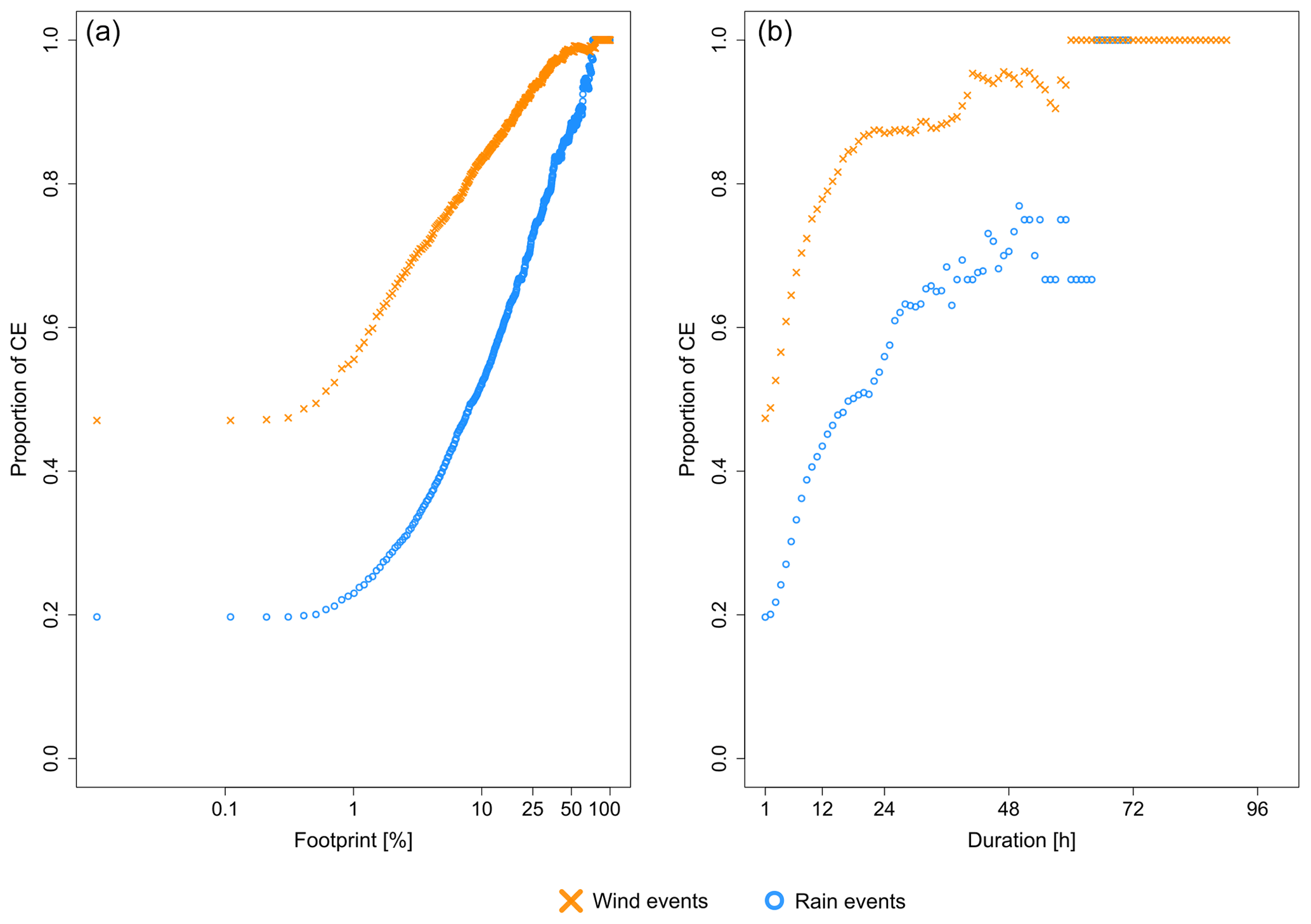
Figure A1Proportion of compound wind–precipitation clusters among wind clusters (orange) and precipitation clusters (blue) depending on (a) footprint and (b) duration of the hazard clusters.
Over the study area, the proportion of compound wind–precipitation clusters among the precipitation clusters detected is 20 %, while 47 % of the wind clusters are compound hazard clusters. However, this proportion is variable across Great Britain. Figure A2 displays the fraction of compound hazard clusters among (a) wind clusters and (b) precipitation clusters. It highlights the spatial variability of compound cluster prevalence. Orography probably plays an important role in the geographical features that may influence the frequency of compound hazard clusters among precipitation and wind clusters. The frequency of compound wind–precipitation clusters is the highest in mountainous areas, while lowlands of the west coast have a much lower frequency of compound wind–precipitation clusters among both precipitation and wind clusters.

Figure A2Compound hazard (wind–precipitation) cluster proportion among (a) wind clusters and (b) precipitation clusters during the period 1979–2019 in Great Britain. Data from ERA5 (Hersbach et al., 2018).
However, compound wind–precipitation clusters are more prevalent among the most intense hazard clusters. The latter represents 58 of the 100 most intense precipitation clusters and 95 of the 100 most intense wind clusters. The intensity of precipitation and wind clusters is assessed with the intensity attributes presented in Table 1. The proportion of compound wind–precipitation clusters increases with duration and footprint for both precipitation and wind clusters (Fig. A1).
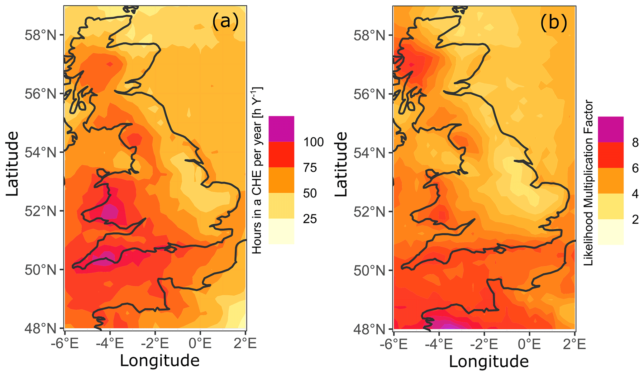
Figure A3Hotspots for compound wind–precipitation clusters in Great Britain showing (a) the average number of hours in a compound hazard cluster in a year for 1979–2019 and (b) the likelihood multiplication factor (LMF) that quantifies the influence of the dependence between wind and rain clusters on the estimation of the probability of occurrence of compound hazard clusters. Data from ERA5 (Hersbach et al., 2018).
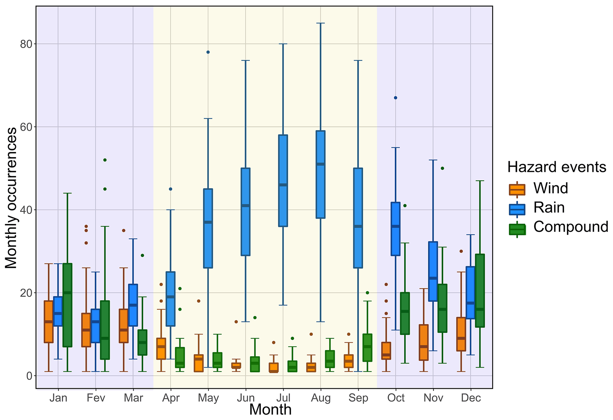
Figure A4Box plots of the monthly number of wind (dark orange), rain (blue), and compound (green) hazard clusters in Great Britain over the period 1979–2019. Background colours represent the two seasons. Data from ERA5 (Hersbach et al., 2018).
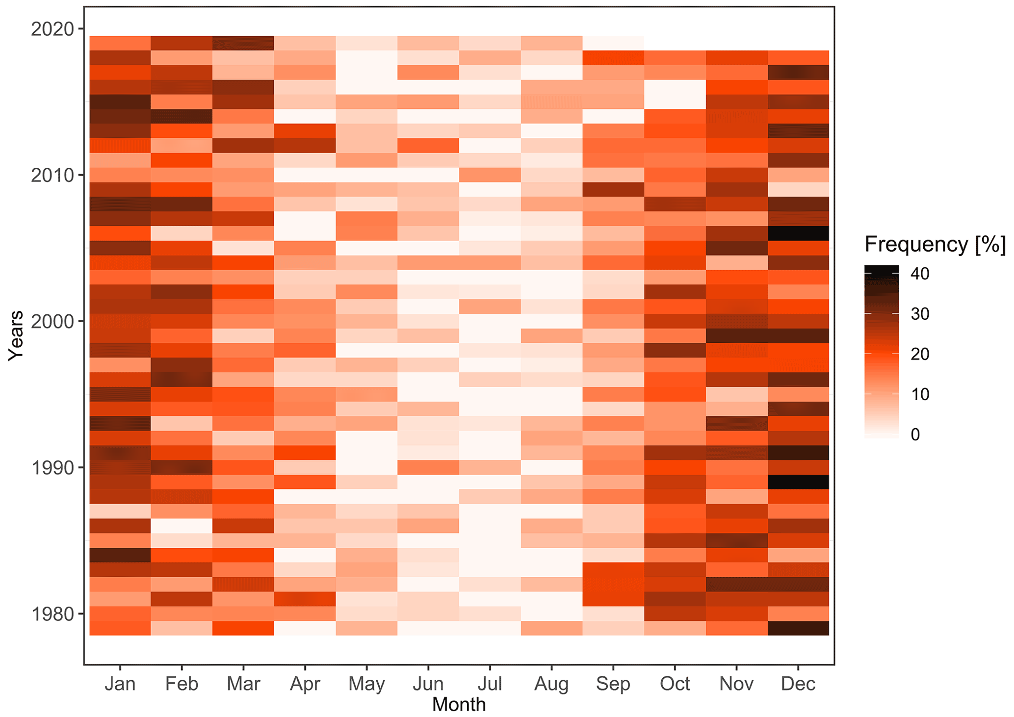
Figure A5Monthly fraction of compound hazard clusters among the total number of clusters (wind only+rain only+compound clusters) for that month for 1979–2019 over the study area. Each tile represents a month–year pair; darker tiles mean that the fraction of compound hazard clusters is greater.
As the duration of compound wind–precipitation clusters highly varies, their frequency of occurrence in the study area is assessed by counting the number of hours in a compound cluster (as defined in Sect. 4.3) at each grid cell. The average number of hours per year in a compound cluster for 1979–2019 is displayed in Fig. A3a. This value varies between 20 and 95 h in the study area. Figure A3a highlights regions more likely to be affected by compound wind–precipitation clusters with hotspots in mountainous areas (as for Fig. A2). Nevertheless, the southeastern coast of Great Britain is the primary hotspot for compound wind–precipitation clusters. The frequency of compound clusters gradually decreases eastward from Cornwall and Wales toward Anglia and East Midlands, showing a west–east decreasing gradient across all Great Britain. A similar pattern has been found for extreme precipitation (Blenkinsop et al., 2017) and compound flooding (Hendry et al., 2019). The prevailing direction of cyclonic weather systems and orography partly explains this pattern for compound wind–precipitation clusters (Hulme and Barrow, 1997).
The dependence between extreme wind and extreme precipitation (w, p) can influence the estimation of the joint return period. The influence of the dependence between extreme wind and extreme rainfall cluster occurrence is quantified using the likelihood multiplication factor (LMF) (Zscheischler and Seneviratne, 2017). The LMF is the ratio between the joint return period considering the two variables dependently (Tdep) and independently (Tind) of each other (Manning et al., 2019):
The likelihood multiplication factor (LMF) quantifies the influence of the dependence between wind clusters and rain clusters on estimating the frequency of compound wind–precipitation clusters (Fig. A3a). The LMF (Fig. A3b) shows the strength of the dependence between wind and rain clusters. The LMF is > 1.0 in all parts of the study area, suggesting that rain and wind clusters do not occur independently. The LMF is particularly high along the southern coast of Great Britain, in the British Channel, and in northwestern France. While occurrences of compound wind–precipitation clusters exhibit an east–west pattern, the strength of the dependence between wind and rain hazard clusters has a south–north pattern.
The spatial features of compound wind–rain clusters have been identified in Figs. A2 and A3. Spatial disparities in their frequency and their dependence between wind and rain clusters have been highlighted. These features also vary in time and with seasons. To characterise the seasonality of single (wind only, rain only) and compound hazard clusters, all hazard clusters have been taken into account and divided into three categories: wind, rain, and compound. Wind clusters that are part of a compound cluster are removed from the category “wind”, while rain clusters that are part of a compound cluster are removed from the category “rain”. Monthly occurrences of these three categories of clusters are displayed in Fig. A4. While occurrences of wind and compound clusters are correlated, with a high season in extended winter (ONDJFM) and a low season in the extended summer (AMJJAS), rain cluster occurrence follows an opposite pattern, with a high season in AMJJAS and a low season in ONDJFM. Around 82 % of all recorded compound hazard clusters occur during the extended winter.
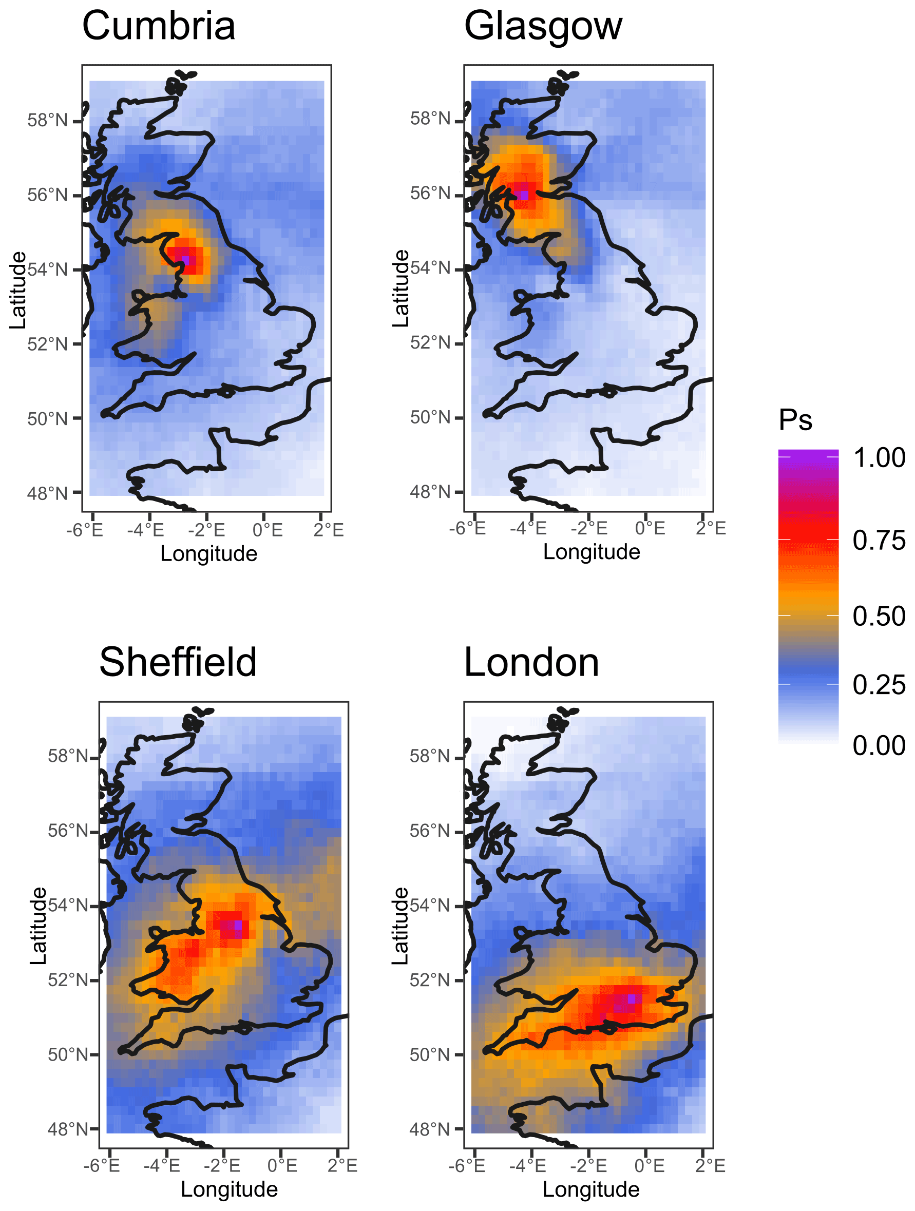
Figure A6Spatial dependence of compound wind–rain occurrence between different sites. Ps is the probability of each grid cell in the study area to be in a compound wind–precipitation cluster, knowing that a given cell of reference is in a compound cluster.
Figure A5 provides a perspective on the seasonality of compound wind–precipitation clusters. It displays the proportion of compound wind–precipitation clusters among all clusters, with a seasonal proportion pattern similar to the one observed in Fig. A4. This suggests that extreme rainfall and extreme wind clusters are more likely to co-occur during the extended winter. One possible explanation is that conditions leading to compound wind–precipitation clusters occur during the extended winter (Hillier et al., 2020). This season coincides with the extratropical season in western Europe (Mailier et al., 2006; Ulbrich et al., 2009; Deroche et al., 2014). Extratropical cyclones can bring several hazards, including strong wind, storm surge, heavy rainfall, and high waves (Frame et al., 2017).
Figures A3–A5 suggest that extratropical cyclones could influence compound wind and precipitation extremes, with a west–east pattern characteristic of the British island (Hulme and Barrow, 1997) and an increase in the frequency of compound events in the extended winter. The influence of cyclonic weather systems coming from the Atlantic on precipitation and wind extremes in Great Britain has been highlighted in previous work (Hawcroft et al., 2012; Dowdy and Catto, 2017). However, this does not mean that every compound hazard cluster occurring during the extended winter is an extratropical cyclone but suggests that such weather systems are drivers of compound wind–precipitation extreme clusters. Other weather systems such as convective storms can also lead to compound wind and precipitation extremes (Zhang et al., 2021).
The spatial dependence between different sites is investigated in Fig. A6. This figure highlights each grid cell's empirical probability to be in a compound wind–precipitation cluster, knowing that a given cell of reference is in a compound cluster (displayed as Ps in Fig. A6). Four locations in Great Britain are taken as cells of reference: Cumbria, Sheffield, London, and Glasgow. The spatial extent of compound wind–precipitation clusters is displayed differently from the one adopted in Sect. 5, highlighting that London is more likely to be in a large-scale cluster than Glasgow. Spatial dependences between places are also visible; for example, compound cluster occurrence in London is associated with compound cluster occurrence in southern England, while compound clusters occurring in Sheffield are more likely to develop over the Midlands and Wales.
The codes used to generate the single and compound hazard clusters in this study were produced with R (https://www.R-project.org/; R Core Team, 2022) and are publicly available on Zenodo (https://doi.org/10.5281/zenodo.6555825; Tilloy, 2022).
The ERA5 data were downloaded from the Copernicus Climate Data Store (2020) (https://cds.climate.copernicus.eu/cdsapp#!/dataset/reanalysis-era5-land). Input, intermediary, and output data used in this article are available in Tilloy (2021) (https://doi.org/10.5281/zenodo.4906264).
There are four parts to the Supplement to this article.
-
Supplement 1: Supplementary information on the DBSCAN algorithm.
-
Supplement 2: Sensitivity analysis of the spatiotemporal identification of compound hazards (SI–CH) procedure.
-
Supplement 3: ERA5 Hazard Clusters Database 1979–2019 (3.1. Wind, 3.2. Precipitation, 3.3. Compound hazards).
-
Supplement 4: Great Britain Significant Weather Events Catalogue 1979–2019.
The supplement related to this article is available online at: https://doi.org/10.5194/esd-13-993-2022-supplement.
AT, BDM, and AJL worked on the conceptualisation and methodology of the article. AT implemented the analysis, prepared the data, and wrote the draft. AT and BDM worked on visualisation and data curation. BDM edited the original draft.
The contact author has declared that neither they nor their co-authors have any competing interests.
Publisher's note: Copernicus Publications remains neutral with regard to jurisdictional claims in published maps and institutional affiliations. Note that our ERA5 Hazard Clusters Database 1979–2019 contains modified ERA5 data from the Copernicus Climate Change Service Information and that neither the European Commission nor ECMWF is responsible for any use that may be made of the Copernicus Information or data it contains.
The authors gratefully acknowledge the detailed comments of two anonymous reviewers.
Aloïs Tilloy was funded by an EDF Energy R & D PhD studentship.
This paper was edited by Rui A. P. Perdigão and reviewed by two anonymous referees.
AghaKouchak, A., Chiang, F., Huning, L. S., Love, C. A., Mallakpour, I., Mazdiyasni, O., Moftakhari, H., Papalexiou, S. M., Ragno, E., and Sadegh, M.: Climate extremes and compound hazards in a warming world, Annu. Rev. Earth Planet. Sci., 48, 519–548, https://doi.org/10.1146/annurev-earth-071719-055228, 2020.
Agrawal, K. P., Garg, S., Sharma, S., and Patel, P.: Development and validation of OPTICS based spatio-temporal clustering technique, Inf. Sci., 369, 388–401, https://doi.org/10.1016/j.ins.2016.06.048, 2016.
Angélil, O., Perkins-Kirkpatrick, S., Alexander, L. V., Stone, D., Donat, M. G., Wehner, M., Shiogama, H., Ciavarella, A., and Christidis, N.: Comparing regional precipitation and temperature extremes in climate model and reanalysis products, Weather Clim. Extrem., 13, 35–43, https://doi.org/10.1016/j.wace.2016.07.001, 2016.
Ansari, M. Y., Ahmad, A., Khan, S. S., Bhushan, G., and Mainuddin: Spatiotemporal clustering: a review, Artif. Intell. Rev., 53, 2381–2423, https://doi.org/10.1007/s10462-019-09736-1, 2020.
Bach, B., Dragicevic, P., Archambault, D., Hurter, C., and Carpendale, S.: A review of temporal data visualizations based on space-time cube operations, in Eurographics Conference on Visualization (EuroVis), June 2014, Swansea, Wales, UK, 23–41, https://doi.org/10.2312/eurovisstar.20141171, 2014.
Balch, J. K., Iglesias, V., Braswell, A. E., Rossi, M. W., Joseph, M. B., Mahood, A. L., Shrum, T. R., White, C. T., Scholl, V. M., McGuire, B., Karban, C., Buckland, M., and Travis, W. R.: Social-environmental extremes: Rethinking extraordinary events as outcomes of interacting biophysical and social systems, Earth's Future, 8, e2019EF001319, https://doi.org/10.1029/2019EF001319, 2020.
Barton, Y., Giannakaki, P., von Waldow, H., Chevalier, C., Pfahl, S., and Martius, O.: Clustering of regional-scale extreme precipitation events in southern Switzerland, Mon. Weather Rev., 144, 347–369, https://doi.org/10.1175/MWR-D-15-0205.1, 2016.
Beck, H. E., Zimmermann, N. E., McVicar, T. R., Vergopolan, N., Berg, A., and Wood, E. F.: Present and future Köppen-Geiger climate classification maps at 1-km resolution, Sci. Data, 5, 1–12, https://doi.org/10.1038/sdata.2018.214, 2018.
Beck, H. E., Pan, M., Roy, T., Weedon, G. P., Pappenberger, F., van Dijk, A. I. J. M., Huffman, G. J., Adler, R. F., and Wood, E. F.: Daily evaluation of 26 precipitation datasets using Stage-IV gauge-radar data for the CONUS, Hydrol. Earth Syst. Sci., 23, 207–224, https://doi.org/10.5194/hess-23-207-2019, 2019.
Birant, D. and Kut, A.: ST-DBSCAN: An algorithm for clustering spatial-temporal data, Data Knowl. Eng., 60, 208–221, https://doi.org/10.1016/j.datak.2006.01.013, 2007.
Blenkinsop, S., Lewis, E., Chan, S. C., and Fowler, H. J.: Quality-control of an hourly rainfall dataset and climatology of extremes for the UK, Int. J. Climatol., 37, 722–740, https://doi.org/10.1002/joc.4735, 2017.
Blöschl, G. and Sivapalan, M.: Scale issues in hydrological modelling: A review, Hydrol. Process., 9, 251–290, https://doi.org/10.1002/hyp.3360090305, 1995.
Brakenridge, G. R.: Global Active Archive of Large Flood Events. Dartmouth Flood Observatory, University of Colorado, USA, http://floodobservatory.colorado.edu/Archives/, last access: 29 June 2021.
Brönnimann, S., Allan, R., Atkinson, C., Buizza, R., Bulygina, O., Dahlgren, P., Dee, D., Dunn, R., Gomes, P., John, V. O., Jourdain, S., Haimberger, L., Hersbsbach, H., Kennedy, J., Poli, P., Pulliainen, J., Rayner, N., Saunders, R., Schulz, J., Sterin, A., Stickler, A., Titchner, H., Valente, M. A., Ventura, C., and Wilkinson, C.: Observations for reanalyses, B. Am. Meteorol. Soc., 99, 1851–1866, https://doi.org/10.1175/BAMS-D-17-0229.1, 2018.
Catto, J. L. and Dowdy, A.: Understanding compound hazards from a weather system perspective, Weather Clim. Extrem., 32, 100313, https://doi.org/10.1016/j.wace.2021.100313, 2021.
Chazette, P., Flamant, C., Raut, J., Totems, J., and Shang, X.: Tropical moisture enriched storm tracks over the Mediterranean and their link with intense rainfall in the Cevennes-Vivarais area during HyMeX, Q. J. Roy. Meteorol. Soc., 142, 320–334, https://doi.org/10.1002/qj.2674, 2016.
Copernicus Climate Data Store: ERA5-Land hourly data, Copernicus Climate Data Store [data set], https://cds.climate.copernicus.eu/cdsapp#!/dataset/reanalysis-era5-land (last access: 18 March 2022), 2020.
Cornes, R. C., van der Schrier, G., van den Besselaar, E. J. M., and Jones, P. D.: An Ensemble Version of the E-OBS temperature and precipitation data sets, J. Geophys. Res.-Atmos., 123, 9391–9409, https://doi.org/10.1029/2017JD028200, 2018.
CRED – Centre for Research on the Epidemiology of Disasters: EM-DAT – The Emergency Events Database, Univ. Catholique Louvain, https://www.emdat.be/, last access: 22 December 2020.
Cressie, N. A. C.: Statistics for Spatial Data, John Wiley & Sons, Inc., New York, https://doi.org/10.1002/9781119115151, 1993.
De Angeli, S., Malamud, B. D., Rossi, L., Taylor, F. E., Trasforini, E., and Rudari, R.: A multi-hazard framework for spatial-temporal impact analysis, Int. J. Disast. Risk Reduct., 73, 102829, https://doi.org/10.1016/j.ijdrr.2022.102829, 2022.
Deroche, M. S., Choux, M., Codron, F., and Yiou, P.: Three variables are better than one: Detection of european winter windstorms causing important damages, Nat. Hazards Earth Syst. Sci., 14, 981–993, https://doi.org/10.5194/nhess-14-981-2014, 2014.
Diederen, D., Liu, Y., Gouldby, B., Diermanse, F., and Vorogushyn, S.: Stochastic generation of spatially coherent river discharge peaks for large-scale, event-based flood risk assessment, Nat. Hazards Earth Syst. Sci., 19, 1041–1053, https://doi.org/10.5194/nhess-19-1041-2019, 2019.
Donat, M. G., Sillmann, J., Wild, S., Alexander, L. V., Lippmann, T., and Zwiers, F. W.: Consistency of temperature and precipitation extremes across various global gridded in situ and reanalysis datasets, J. Climate, 27, 5019–5035, https://doi.org/10.1175/JCLI-D-13-00405.1, 2014.
Dowdy, A. J. and Catto, J. L.: Extreme weather caused by concurrent cyclone, front and thunderstorm occurrences, Sci. Rep., 7, 1–8, https://doi.org/10.1038/srep40359, 2017.
Eden, P.: Great British Weather Disasters, Continuum, London, ISBN 10 1441145915, ISBN 13 978-1441145918, 2008.
Ester, M., Kriegel, H.-P., Sander, J., and Xu, X.: A density-based algorithm for discovering clusters in large spatial databases with noise, in: KDD-1996 Proceedings of the Second International Conference on Knowledge Discovery and Data Mining, 2–4 August 1996, Portland, Oregon, 226–231, https://www.aaai.org/Papers/KDD/1996/KDD96-037.pdf (last access: 1 May 2022), 1996.
Fan, X., Scaringi, G., Korup, O., West, A. J., van Westen, C. J., Tanyas, H., Hovius, N., Hales, T. C., Jibson, R. W., Allstadt, K. E., Zhang, L., Evans, S. G., Xu, C., Li, G., Pei, X., Xu, Q., and Huang, R.: Earthquake-induced chains of geologic hazards: Patterns, mechanisms, and impacts, Rev. Geophys., 57, 421–503, https://doi.org/10.1029/2018RG000626, 2019.
Frame, T., Harrisonm, G., Hewson, T., and Roberts, N.: Meteorological Risk: extra-tropical cyclones, tropical cyclones and convective storms, in: Science for Disaster Risk Management 2017: Knowing Better and Losing Less, Publications Office of the European Union, Luxembourg, 246–256, https://doi.org/10.2788/842809, 2017.
García-Herrera, R., Garrido-Perez, J. M., Barriopedro, D., Ordóñez, C., Vicente-Serrano, S. M., Nieto, R., Gimeno, L., Sorí, R., and Yiou, P.: The European 2016/17 drought, J. Climate, 32, 3169–3187, https://doi.org/10.1175/JCLI-D-18-0331.1, 2019.
Georgoulas, G., Konstantaras, A., Katsifarakis, E., Stylios, C. D., Maravelakis, E., and Vachtsevanos, G. J.: “Seismic-mass” density-based algorithm for spatio-temporal clustering, Expert Syst. Appl., 40, 4183–4189, https://doi.org/10.1016/j.eswa.2013.01.028, 2013.
Gill, J. C. and Malamud, B. D.: Reviewing and visualizing the interactions of natural hazards, Rev. Geophys., 52, 680–722, https://doi.org/10.1002/2013RG000445, 2014.
Gleixner, S., Demissie, T., and Diro, G. T.: Did ERA5 improve temperature and precipitation reanalysis over East Africa?, Atmosphere (Basel), 11, 996, https://doi.org/10.3390/atmos11090996, 2020.
Hahsler, M., Piekenbrock, M., and Doran, D.: dbscan: Fast density-based clustering with R, J. Stat. Softw., 91, 1–30, https://doi.org/10.18637/jss.v091.i01, 2019.
Hawcroft, M. K., Shaffrey, L. C., Hodges, K. I., and Dacre, H. F.: How much Northern Hemisphere precipitation is associated with extratropical cyclones?, Geophys. Res. Lett., 39, L24809, https://doi.org/10.1029/2012GL053866, 2012.
Hendry, A., Haigh, I. D., Nicholls, R. J., Winter, H. C., Neal, R., Wahl, T., Joly-Laugel, A., and Darby, S. E.: Assessing the characteristics and drivers of compound flooding events around the UK coast, Hydrol. Earth Syst. Sci., 23, 3117–3139, https://doi.org/10.5194/hess-23-3117-2019, 2019.
Hersbach, H., Bell, B., Berrisford, P., Biavati, G., Horányi, A., Muñoz Sabater, J., Nicolas, J., Peubey, C., Radu, R., Rozum, I., Schepers, D., Simmons, A., Soci, C., Dee, D., and Thépaut, J.-N.: ERA5 hourly data on single levels from 1979 to present. Copernicus Climate Change Service (C3S) Climate Data Store (CDS), https://doi.org/10.24381/cds.adbb2d47, 2018.
Hersbach, H., Bell, B., Berrisford, P., Horányi, A., Sabater, J. M., Nicolas, J., Radu, R., Schepers, D., Simmons, A., Soci, C., and Dee, D.: Global reanalysis: goodbye ERA-Interim, hello ERA5, ECMWF Newslett., 159, 17–24, https://doi.org/10.21957/vf291hehd7, 2019.
Hersbach, H., Bell, B., Berrisford, P., Hirahara, S., Horányi, A., Muñoz-Sabater, J., Nicolas, J., Peubey, C., Radu, R., Schepers, D., Simmons, A., Soci, C., Abdalla, S., Abellan, X., Balsamo, G., Bechtold, P., Biavati, G., Bidlot, J., Bonavita, M., Chiara, G., Dahlgren, P., Dee, D., Diamantakis, M., Dragani, R., Flemming, J., Forbes, R., Fuentes, M., Geer, A., Haimberger, L., Healy, S., Hogan, R. J., Hólm, E., Janisková, M., Keeley, S., Laloyaux, P., Lopez, P., Lupu, C., Radnoti, G., Rosnay, P., Rozum, I., Vamborg, F., Villaume, S., and Thépaut, J.: The ERA5 global reanalysis, Q. J. Roy. Meteorol. Soc., 146, 1999–2049, https://doi.org/10.1002/qj.3803, 2020.
Hillier, J. K., Matthews, T., Wilby, R. L., and Murphy, C.: Multi-hazard dependencies can increase or decrease risk, Nat. Clim. Change, 10, 595–598, https://doi.org/10.1038/s41558-020-0832-y, 2020.
Holley, D. M., Dorling, S. R., Steele, C. J., and Earl, N.: A climatology of convective available potential energy in Great Britain, Int. J. Climatol., 34, 3811–3824, https://doi.org/10.1002/joc.3976, 2014.
Huang, W., Xu, S., Yan, Y., and Zipf, A.: An exploration of the interaction between urban human activities and daily traffic conditions: A case study of Toronto, Canada, Cities, 84, 8–22, https://doi.org/10.1016/j.cities.2018.07.001, 2019.
Hulme, M. and Barrow, E.: Climates of the British Isles, Routledge, London, https://doi.org/10.4324/9781315870793, 1997.
Huntingford, C., Marsh, T., Scaife, A. A., Kendon, E. J., Hannaford, J., Kay, A. L., Lockwood, M., Prudhomme, C., Reynard, N. S., Parry, S., Lowe, J. A., Screen, J. A., Ward, H. C., Roberts, M., Stott, P. A., Bell, V. A., Bailey, M., Jenkins, A., Legg, T., Otto, F. E. L., Massey, N., Schaller, N., Slingo, J., and Allen, M. R.: Potential influences on the United Kingdom's floods of winter 2013/14, Nat. Clim. Change, 4, 769–777, https://doi.org/10.1038/nclimate2314, 2014.
Iordanidou, V., Koutroulis, A. G., and Tsanis, I. K.: Investigating the relationship of lightning activity and rainfall: A case study for Crete Island, Atmos. Res., 172–173, 16–27, https://doi.org/10.1016/j.atmosres.2015.12.021, 2016.
Joyce, R. J., Janowiak, J. E., Arkin, P. A., and Xie, P.: CMORPH: A method that produces global precipitation estimates from passive microwave and infrared data at high spatial and temporal resolution, J. Hydrometeorol., 5, 487–503, https://doi.org/10.1175/1525-7541(2004)005<0487:CAMTPG>2.0.CO;2, 2004.
Kassambara, A.: Practical Guide to Cluster Analysis in R: Unsupervised machine learning, STHDA, Poland, ISBN 10 1542462703, ISBN 13 978-1542462709, 2017.
Kendon, E. J., Ban, N., Roberts, N. M., Fowler, H. J., Roberts, M. J., Chan, S. C., Evans, J. P., Fosser, G., and Wilkinson, J. M.: Do convection-permitting regional climate models improve projections of future precipitation change?, B. Am. Meteorol. Soc., 98, 79–93, https://doi.org/10.1175/BAMS-D-15-0004.1, 2017.
Kholodovsky, V. and Liang, X.-Z.: A generalized spatio-temporal threshold clustering method for identification of extreme event patterns, Adv. Stat. Clim. Meteorol. Oceanogr., 7, 35–52, https://doi.org/10.5194/ascmo-7-35-2021, 2021.
Klerk, W. J., Winsemius, H. C., van Verseveld, W. J., Bakker, A. M. R., and Diermanse, F. L. M.: The co-incidence of storm surges and extreme discharges within the Rhine–Meuse Delta, Environ. Res. Lett., 10, 035005, https://doi.org/10.1088/1748-9326/10/3/035005, 2015.
Lancaster, J.: What is the right scale? Encouraging fruitful engagement for ecology with ecohydraulics, J. Ecohydraulics, 3, 63–76, https://doi.org/10.1080/24705357.2018.1535260, 2018.
Leonard, M., Westra, S., Phatak, A., Lambert, M., van den Hurk, B. J., McInnes, K., Risbey, J., Schuster, S., Jakob, D., and Stafford-Smith, M.: A compound event framework for understanding extreme impacts, Wiley Interdisciplin. Rev. Clim. Change, 5, 113–128, https://doi.org/10.1002/wcc.252, 2014.
Mahto, S. S. and Mishra, V.: Does ERA-5 Outperform Other Reanalysis Products for Hydrologic Applications in India?, J. Geophys. Res.-Atmos., 124, 9423–9441, https://doi.org/10.1029/2019JD031155, 2019.
Mailier, P. J., Stephenson, D. B., Ferro, C. A. T., and Hodges, K. I.: Serial clustering of extratropical cyclones, Mon. Weather Rev., 134, 2224–2240, https://doi.org/10.1175/MWR3160.1, 2006.
Manning, C., Widmann, M., Bevacqua, E., Van Loon, A. F., Maraun, D., and Vrac, M.: Increased probability of compound long-duration dry and hot events in Europe during summer (1950–2013), Environ. Res. Lett., 14, 094006, https://doi.org/10.1088/1748-9326/ab23bf, 2019.
Martius, O., Pfahl, S., and Chevalier, C.: A global quantification of compound precipitation and wind extremes, Geophys. Res. Lett., 43, 7709–7717, https://doi.org/10.1002/2016GL070017, 2016.
Mastrantonas, N., Herrera-Lormendez, P., Magnusson, L., Pappenberger, F., and Matschullat, J.: Extreme precipitation events in the Mediterranean: Spatiotemporal characteristics and connection to large-scale atmospheric flow patterns, Int. J. Climatol., 41, 2710–2728, https://doi.org/10.1002/joc.6985, 2020.
Met Office: Past weather events, https://www.metoffice.gov.uk/weather/learn-about/past-uk-weather-events, last access: 1 October 2020.
Milligan, G. W. and Cooper, M. C.: Methodology review: Clustering methods, Appl. Psychol. Meas., 11, 329–354, https://doi.org/10.1177/014662168701100401, 1987.
Minola, L., Zhang, F., Azorin-Molina, C., Pirooz, A. A. S., Flay, R. G. J., Hersbach, H., and Chen, D.: Near-surface mean and gust wind speeds in ERA5 across Sweden: towards an improved gust parametrization, Clim. Dynam., 55, 887–907, https://doi.org/10.1007/s00382-020-05302-6, 2020.
Molina, M. O., Gutiérrez, C., and Sánchez, E.: Comparison of ERA5 surface wind speed climatologies over Europe with observations from the HadISD dataset, Int. J. Climatol. 41, 4864–4878, https://doi.org/10.1002/joc.7103, 2021.
Naylor, L. A., Spencer, T., Lane, S. N., Darby, S. E., Magilligan, F. J., Macklin, M. G., and Möller, I.: Stormy geomorphology: geomorphic contributions in an age of climate extremes, Earth Surf. Proc. Land., 42, 166–190, https://doi.org/10.1002/esp.4062, 2017.
Nitschke, M., Tucker, G. R., Hansen, A. L., Williams, S., Zhang, Y., and Bi, P.: Impact of two recent extreme heat episodes on morbidity and mortality in Adelaide, South Australia: a case-series analysis, Environ. Health, 10, 42, https://doi.org/10.1186/1476-069X-10-42, 2011.
ONS – Office for National Statistics: NUTS1 Regions, https://www.ons.gov.uk/methodology/geography/ukgeographies/eurostat, last access: 29 June 2021.
Orlanski, I.: A rational subdivision of scales for atmospheric processes, Am. Meteorol. Soc., 56, 527–530, 1975.
Pfahl, S. and Wernli, H.: Quantifying the relevance of cyclones for precipitation extremes, J. Climate, 25, 6770–6780, https://doi.org/10.1175/JCLI-D-11-00705.1, 2012.
Pinto, J. G., Karremann, M. K., Born, K., Della-Marta, P. M., and Klawa, M.: Loss potentials associated with European windstorms under future climate conditions, Clim. Res., 54, 1–20, https://doi.org/10.3354/cr01111, 2012.
Rahman, M. S., Yang, R., and Di, L.: Clustering Indian Ocean tropical cyclone tracks by the standard deviational ellipse, Climate, 6, 39, https://doi.org/10.3390/cli6020039, 2018.
Ramsay, H. A., Camargo, S. J., and Kim, D.: Cluster analysis of tropical cyclone tracks in the Southern Hemisphere, Clim. Dynam., 39, 897–917, https://doi.org/10.1007/s00382-011-1225-8, 2012.
Raveh-Rubin, S. and Wernli, H.: Large-scale wind and precipitation extremes in the Mediterranean: A climatological analysis for 1979–2012, Q. J. Roy. Meteorol. Soc., 141, 2404–2417, https://doi.org/10.1002/qj.2531, 2015.
R Core Team: R: A Language and Environment for Statistical Computing, R Foundation for Statistical Computing, Vienna, Austria, https://www.R-project.org/, last access: 1 May 2022.
Ridder, N. N., Pitman, A. J., Westra, S., Ukkola, A., Do, H. X., Bador, M., Hirsch, A. L., Evans, J. P., Di Luca, A., and Zscheischler, J.: Global hotspots for the occurrence of compound events, Nat. Commun., 11, 5956, https://doi.org/10.1038/s41467-020-19639-3, 2020.
Rigo, T., Berenguer, M., and del Llasat, M. C.: An improved analysis of mesoscale convective systems in the western Mediterranean using weather radar, Atmos. Res., 227, 147–156, https://doi.org/10.1016/j.atmosres.2019.05.001, 2019.
Rivoire, P., Martius, O., and Naveau, P.: A comparison of moderate and extreme ERA-5 Daily precipitation with two observational data sets, Earth Space Sci., 8, 1–23, https://doi.org/10.1029/2020EA001633, 2021.
Sadegh, M., Moftakhari, H. R., Gupta, H. V., Ragno, E., Mazdiyasni, O., Sanders, B. F., Matthew, R. A., and AghaKouchak, A.: Multihazard scenarios for analysis of compound extreme events, Geophys. Res. Lett., 45, 5470–5480, https://doi.org/10.1029/2018GL077317, 2018.
Saha, S., Moorthi, S., Pan, H. L., Wu, X., Wang, J., Nadiga, S., Tripp, P., Kistler, R., Woollen, J., Behringer, D., Liu, H., Stokes, D., Grumbine, R., Gayno, G., Wang, J., Hou, Y. T., Chuang, H. Y., Juang, H. M. H., Sela, J., Iredell, M., Treadon, R., Kleist, D., Van Delst, P., Keyser, D., Derber, J., Ek, M., Meng, J., Wei, H., Yang, R., Lord, S., Van Den Dool, H., Kumar, A., Wang, W., Long, C., Chelliah, M., Xue, Y., Huang, B., Schemm, J. K., Ebisuzaki, W., Lin, R., Xie, P., Chen, M., Zhou, S., Higgins, W., Zou, C. Z., Liu, Q., Chen, Y., Han, Y., Cucurull, L., Reynolds, R. W., Rutledge, G., and Goldberg, M.: The NCEP climate forecast system reanalysis, B. Am. Meteorol. Soc., 91, 1015–1057, https://doi.org/10.1175/2010BAMS3001.1, 2010.
Schneider, D. C.: Quantitative Ecology: Spatial and Temporal Scaling, Elsevier Inc., Oxford, UK, https://doi.org/10.1016/C2009-0-02445-3, 1994.
Sedlmeier, K., Feldmann, H., and Schädler, G.: Compound summer temperature and precipitation extremes over central Europe, Theor. Appl. Climatol., 131, 1493–1501, https://doi.org/10.1007/s00704-017-2061-5, 2018.
Sharifi, E., Eitzinger, J., and Dorigo, W.: Performance of the state-of-the-art gridded precipitation products over mountainous terrain: A regional study over Austria, Remote Sens., 11, 1–20, https://doi.org/10.3390/rs11172018, 2019.
Shi, Z. and Pun-Cheng, L.: Spatiotemporal Data Clustering: A survey of methods, ISPRS Int. J. Geo-Inform., 8, 112, https://doi.org/10.3390/ijgi8030112, 2019.
Skøien, J. O., Blöschl, G., and Western, A. W.: Characteristic space scales and timescales in hydrology, Water Resour. Res., 39, 1304, https://doi.org/10.1029/2002WR001736, 2003.
Skok, G., Žagar, N., Honzak, L., Žabkar, R., Rakovec, J., and Ceglar, A.: Precipitation intercomparison of a set of satellite- and raingauge-derived datasets, ERA Interim reanalysis, and a single WRF regional climate simulation over Europe and the North Atlantic, Theor. Appl. Climatol., 123, 217–232, https://doi.org/10.1007/s00704-014-1350-5, 2016.
Spinoni, J., Barbosa, P., Bucchignani, E., Cassano, J., Cavazos, T., Cescatti, A., Christensen, J. H., Christensen, O. B., Coppola, E., Evans, J. P., Forzieri, G., Geyer, B., Giorgi, F., Jacob, D., Katzfey, J., Koenigk, T., Laprise, R., Lennard, C. J., Kurnaz, M. L., Li, D., Llopart, M., McCormick, N., Naumann, G., Nikulin, G., Ozturk, T., Panitz, H., Rocha, R. P., Solman, S. A., Syktus, J., Tangang, F., Teichmann, C., Vautard, R., Vogt, J. V., Winger, K., Zittis, G., and Dosio, A.: Global exposure of population and land-use to meteorological droughts under different warming levels and SSPs: a CORDEX-based study, Int. J. Climatol., 41, 6825–6853, https://doi.org/10.1002/joc.7302, 2021.
Strauss, C., Rosa, M. B., and Stephany, S.: Spatio-temporal clustering and density estimation of lightning data for the tracking of convective events, Atmos. Res., 134, 87–99, https://doi.org/10.1016/j.atmosres.2013.07.008, 2013.
Sutanto, S. J., Vitolo, C., Di Napoli, C., D'Andrea, M., and Van Lanen, H. A. J.: Heatwaves, droughts, and fires: Exploring compound and cascading dry hazards at the pan-European scale, Environ. Int., 134, 105276, https://doi.org/10.1016/j.envint.2019.105276, 2020.
Tarek, M., Brissette, F. P., and Arsenault, R.: Evaluation of the ERA5 reanalysis as a potential reference dataset for hydrological modelling over North America, Hydrol. Earth Syst. Sci., 24, 2527–2544, https://doi.org/10.5194/hess-24-2527-2020, 2020.
Temme, A., Guzzetti, F., Samia, J., and Mirus, B. B.: The future of landslides' past – a framework for assessing consecutive landsliding systems, Landslides, 17, 1519–1528, https://doi.org/10.1007/s10346-020-01405-7, 2020.
Tencer, B., Weaver, A., and Zwiers, F.: Joint occurrence of daily temperature and precipitation extreme events over Canada, J. Appl. Meteorol. Clim., 53, 2148–2162, https://doi.org/10.1175/JAMC-D-13-0361.1, 2014.
Tencer, B., Bettolli, M. L., and Rusticucci, M.: Compound temperature and precipitation extreme events in southern South America: Associated atmospheric circulation, and simulations by a multi-RCM ensemble, Clim. Res., 68, 183–199, https://doi.org/10.3354/cr01396, 2016.
Tilloy, A.: Wind and Precipitation Extremes in Great Britain (1979–2019) to apply the methodology for Spatiotemporal Identification of Compound Hazards, Zenodo [data set], https://doi.org/10.5281/zenodo.4906264, 2021.
Tilloy, A.: Alowis/SI-CH: A methodology for the spatiotemporal identification of compound hazards, Zenodo [code], https://doi.org/10.5281/zenodo.6555825, 2022.
Tilloy, A., Malamud, B. D., Winter, H., and Joly-Laugel, A.: A review of quantification methodologies for multi-hazard interrelationships, Earth-Sci. Rev., 196, 102881, https://doi.org/10.1016/j.earscirev.2019.102881, 2019.
Ulbrich, U., Leckebusch, G. C., and Pinto, J. G.: Extra-tropical cyclones in the present and future climate: A review, Theor. Appl. Climatol., 96, 117–131, https://doi.org/10.1007/s00704-008-0083-8, 2009.
Visser-Quinn, A., Beevers, L., Collet, L., Formetta, G., Smith, K., Wanders, N., Thober, S., Pan, M., and Kumar, R.: Spatio-temporal analysis of compound hydro-hazard extremes across the UK, Adv. Water Resour., 130, 77–90, https://doi.org/10.1016/j.advwatres.2019.05.019, 2019.
Vogel, M. M., Zscheischler, J., Fischer, E. M., and Seneviratne, S. I.: Development of future heatwaves for different hazard thresholds, J. Geophys. Res.-Atmos., 125, e2019JD032070, https://doi.org/10.1029/2019JD032070, 2020.
Vorogushyn, S., Merz, B., Lindenschmidt, K.-E., and Apel, H.: A new methodology for flood hazard assessment considering dike breaches, Water Resour. Res., 46, W08541, https://doi.org/10.1029/2009WR008475, 2010.
Widmann, M. and Bretherton, C. S.: Validation of mesoscale precipitation in the NCEP reanalysis using a new gridcell dataset for the Northwestern United States, J. Climate, 13, 1936–1950, https://doi.org/10.1175/1520-0442(2000)013<1936:VOMPIT>2.0.CO;2, 2000.
WMO – World Meteorological Organization: List of all Variables, https://space.oscar.wmo.int/variables, last access: 17 May 2022.
Xu, D. and Tian, Y.: A comprehensive survey of clustering algorithms, Ann. Data Sci., 2, 165–193, https://doi.org/10.1007/s40745-015-0040-1, 2015.
Yuan, G., Sun, P., Zhao, J., Li, D., and Wang, C.: A review of moving object trajectory clustering algorithms, Artif. Intell. Rev., 47, 123–144, https://doi.org/10.1007/s10462-016-9477-7, 2017.
Yue, S.: The Gumbel logistic model for representing a multivariate storm event, Adv. Water Resour., 24, 179–185, https://doi.org/10.1016/s0309-1708(00)00039-7, 2000.
Zhang, X., Alexander, L., Hegerl, G. C., Jones, P. D., Tank, A. K., Peterson, T. C., Trewin, B., and Zwiers, F. W.: Indices for monitoring changes in extremes based on daily temperature and precipitation data, Wiley Interdisciplin. Rev. Clim. Change, 2, 851–870, 2011.
Zhang, Y., Sun, X., and Chen, C.: Characteristics of concurrent precipitation and wind speed extremes in China, Weather Clim. Extrem., 32, 100322, https://doi.org/10.1016/j.wace.2021.100322, 2021.
Zscheischler, J. and Seneviratne, S. I.: Dependence of drivers affects risks associated with compound events, Sci. Adv., 3, e1700263, https://doi.org/10.1126/sciadv.1700263, 2017.
Zscheischler, J., Mahecha, M. D., Harmeling, S., and Reichstein, M.: Detection and attribution of large spatiotemporal extreme events in Earth observation data, Ecol. Inform., 15, 66–73, https://doi.org/10.1016/j.ecoinf.2013.03.004, 2013.
Zscheischler, J., Martius, O., Westra, S., Bevacqua, E., Raymond, C., Horton, R. M., van den Hurk, B., AghaKouchak, A., Jézéquel, A., Mahecha, M. D., Maraun, D., Ramos, A. M., Ridder, N. N., Thiery, W., and Vignotto, E.: A typology of compound weather and climate events, Nat. Rev. Earth Environ., 1, 333–347, https://doi.org/10.1038/s43017-020-0060-z, 2020.
Zscheischler, J., Naveau, P., Martius, O., Engelke, S., and Raible, C. C.: Evaluating the dependence structure of compound precipitation and wind speed extremes, Earth Syst. Dynam., 12, 1–16, https://doi.org/10.5194/esd-12-1-2021, 2021.
- Abstract
- Introduction
- Spatiotemporal clustering brief background
- Spatiotemporal data and study area
- Methodology: spatiotemporal identification of compound clusters (SI–CH)
- Results
- Discussion
- Conclusion
- Appendix A: Additional exploration of spatiotemporal features of compound wind–precipitation clusters in the ERA5 Hazard Clusters Database 1979–2019
- Code availability
- Data availability
- Author contributions
- Competing interests
- Disclaimer
- Acknowledgements
- Financial support
- Review statement
- References
- Supplement