Sedimentary microplankton distributions are shaped by oceanographically connected areas

Having descended through the water column, microplankton in ocean sediments is representative of the ocean surface environment, where it originated. Sedimentary microplankton is therefore used as an archive of past and present surface oceanographic conditions. However, these particles are advected by turbulent ocean currents during their sinking journey. So far, it is unknown to what extent this particle advection shapes the microplankton composition in sediments. Here we use global simulations of sinking particles in a strongly eddying global ocean model, and define ocean bottom provinces based on the particle surface origin locations. We find that these provinces can be detected in global datasets of sedimentary microplankton assemblages, demonstrating the effect provincialism has on the composition of sedimentary remains of surface plankton. These provinces explain the microplankton composition, in addition to, e.g., the ocean surface environment. Connected provinces have implications for the optimal spatial extent of microplankton sediment sample datasets that are used for palaeoceanographic reconstruction, and for the optimal spatial averaging of sediment samples over global datasets.

1 Introduction

Microplankton communities are sensitive to surface oceanographic conditions in which they live. Their remains are preserved in the sedimentary archive of the ocean basins and are therefore used to reconstruct present and past surface ocean conditions. However, the sedimentary microplankton community is not driven by abiotic climate variables (e.g. temperature or nutrient availability) alone. These climate variables only explain part of the sedimentary species variability, for both dinoflagellate cysts (Zonneveld et al., 2010; Esper and Zonneveld, 2007) and planktic foraminifera (Morey et al., 2005). As a result, there is a large unexplained residual error in relationships between plankton composition and environmental conditions. This impacts the accuracy of the reconstruction of past environmental conditions using microfossil assemblages. Hence, it is crucial to investigate which other processes determine the species distribution in the sedimentary archive, especially when such distributions are used to reconstruct these sea surface variables in the geologic past.

Global surface ocean currents, and the way in which these currents connect the ocean, are shown to shape the plankton community structure near the ocean surface (Jonnson and Watson, 2016; Wilkins et al., 2013; Hellweger, 2014). The connectivity of the two-dimensional (2D) surface ocean flow is well-studied in models (Froyland et al., 2007, 2014; Onink et al., 2019; McAdam and van Sebille, 2018). Floating particles accumulate towards the so-called garbage patches on decadal timescales (Lebreton et al., 2012), which often match well with relatively high concentrations of surface drifters (van Sebille et al., 2012) and microplastics (van Sebille et al., 2015b). In addition to the ocean surface connectivity, the three-dimensional (3D) ocean connectivity is expected to have an influence on the distribution of sedimentary particles.

Studies show that advection of sinking particles in 3D ocean flow has implications for sedimentary microplankton distributions (van Sebille et al., 2015a; Nooteboom et al., 2019; Weyl, 1978; Mollenhauer et al., 2003; Ganssen and Kroon, 1991). An initially uniform distribution of particles at the ocean surface becomes more heterogeneous (i.e. mixed) when these particles are sinking (Monroy et al., 2019; Drótos et al., 2019). At the same time, the influence of ocean currents on sedimentary particle distributions is spatially varying (Nooteboom et al., 2020). Hence, one might expect that the sedimentary archive is shaped by 3D particle advection by ocean currents during the sinking process.

The behaviour of sinking particles in a 3D flow is quite different compared to that in a 2D flow. For instance, a 2D flow is divergent in an upwelling region (which drives the particle convergence in garbage patches), while a 3D flow is non-divergent. However, attracting structures (Bettencourt et al., 2012) and transport barriers (Bettencourt et al., 2015; Chang et al., 2018) of 3D particle paths can also emerge inside the ocean. In this way, particles can cluster in specific areas when they are collected at a 2D surface after their sinking journey (Monroy et al., 2017; Eaton and Fessler, 1994), as is also measured at the ocean subsurface (Mitchell et al., 2008; Logan and Wilkinson, 1990).

In this paper, we investigate how oceanographically disconnected areas shape the sedimentary microplankton composition. We cluster sedimentary sites based on similar ocean surface origin locations of particles that ended up at these sediment sites after their sinking journey. We compare the clusters with well-known features of the ocean flow and detect these clusters in measurements of sedimentary microplankton.

2 Method

2.1 Sedimentary data

We use two global datasets of sedimentary microplankton, one with dinoflagellate cysts (dinocysts; Marret et al., 2019) and the second with planktic foraminifera (Siccha and Kucera, 2017). We use the surface sediment samples from sites south of 65^∘ N (2849 and 4017 sites for the dinocysts and foraminifera respectively) because the OFES ocean model (which is used for particle advection; see below) ends at 75^∘ N, which makes the clustering results at high northern latitudes unreliable. For some statistical analyses, we only consider sites in the Southern Hemisphere (725 and 1858 sites for respectively the dinocysts and foraminifera), in order to limit the total diversity of microplankton species in the datasets. We consider the fraction (i.e. the relative abundance) of microplankton species for every surface sediment sample.

2.2 Clustering methods and particle tracking

The particle tracking results from Nooteboom et al. (2019) provide us with distributions of surface origin locations for a global $\mathrm{1}{}^{\circ }\times \mathrm{1}{}^{\circ }$ grid of sediment sites, for several sinking speeds. We use the results that are obtained in the eddying OFES model (Sasaki et al., 2008; Masumoto et al., 2004) with a sinking speed of 6 m d⁻¹. Results with a sinking speed of 11, 25, and 250 m d⁻¹ can be found in the Supplement. Values of 6 and 11 m d⁻¹ are representative of single sinking dinocysts, 25 m d⁻¹ representative of small aggregates, and 250 m d⁻¹ representative of large aggregates and planktic foraminifera (Anderson et al., 1985; Nooteboom et al., 2019, 2020; van Sebille et al., 2015a). Sinking speeds lower than 6 m d⁻¹ can occur (e.g. due to oxidation of organic material and the development of gas within a shell), which may have an effect on the computed clusters. However, sinking speeds lower than 6 m d⁻¹ are not tested in this paper because the backtracking method is computationally infeasible at lower sinking speeds due to long particle travel times.

The sinking speeds and backtracking analysis from Nooteboom et al. (2019) are specifically designed to be compatible with the life cycle of dinocysts (Nooteboom et al., 2019): particles are released at the bottom of the ocean every 5 d and tracked back in time until they reach 10 m depth, providing a particle distribution at the ocean surface (Fig. 1a). Single foraminifera typically sink at higher velocities than dinocysts (≳100 m d⁻¹), and most of their lateral transport occurs during their lifespan, when they are passively advected while they control their buoyancy and remain at their preferential depth (van Sebille et al., 2015a). However, we assume in this paper that the strength, direction, and “mixing” of planktic foraminifera by ocean currents has a similar spatially varying character compared to sinking dinocysts. We test whether the clustering results match both dinocyst and foraminifera sample datasets.

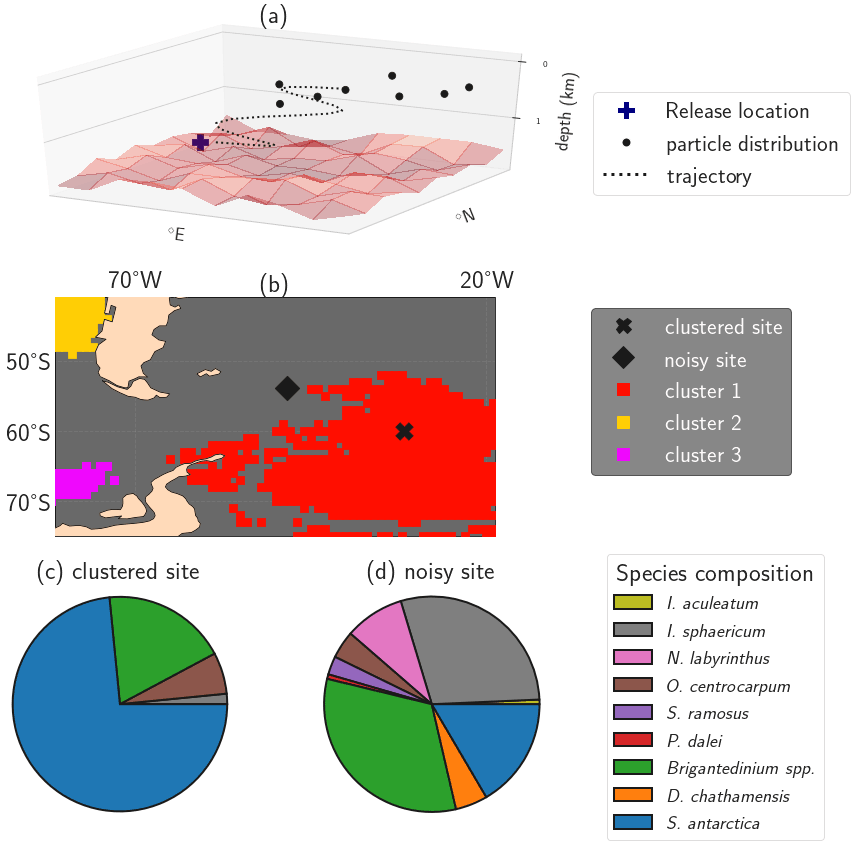
Figure 1 Illustration of the impact of isolated clusters on sedimentary microplankton composition. (a) Illustration of the particle backtrack analysis from Nooteboom et al. (2019), resulting in a particle distribution of origin locations for one sediment site or release location on which the clustering methods are applied (figure adapted from Nooteboom et al., 2020). (b) A (noisy) sediment sample site outside of the isolated clusters (station J299) and a site within oceanographically isolated OPTICS cluster 1 (station J285) in the South Atlantic. (c, d) Pie charts of the dinocyst species composition in the sites from (b). The clustered site contains a species composition which is less biodiverse compared to the noisy site. The Shannon biodiversity indices of respectively the clustered and noisy site are 0.7788 and 1.6842. This illustration uses the same OPTICS clusters as are shown later in Fig. 4.

Our goal is to obtain provinces of sediment sites from the backtracked surface origin locations which are oceanographically (1) disconnected (i.e. provinces between which particles are not likely to travel) and (2) isolated (i.e. provinces with sediment sites which share similar origin locations compared to the sediment sites outside of the province). We quantify these areas by disconnected and isolated clusters of sedimentary sites. Assuming that the flow from 2000 to 2005, as simulated by the OFES model, is representative of the real ocean flow in the past decades (during which the microplankton actually sedimented; Jonkers et al., 2019), we ideally find the disconnectedness and isolation of clusters in the surface sediment sample datasets.

We use two types of clustering techniques. First, hierarchical clustering provides boundaries where sinking particles are less likely to cross (hence it finds oceanographically disconnected areas). This technique starts with the full ocean as only cluster and splits a cluster into two clusters at every iteration (see Appendix A1 for more details). The clusters from this technique can be compared to areas that are known to be oceanographically (dis)connected from each other, and these clusters can be used to test if more similar microplankton species are found within each connected area compared to between connected areas. Advantages of the hierarchical clustering method are that the cluster structure is preserved as more iterations are applied, and it does not require many parameters. The only parameter that the hierarchical clustering uses is the stop criterion (i.e. the iteration number where the algorithm stops with creating new clusters).

Second, we use the Ordering Points To Identify the Clustering Structure (OPTICS) algorithm to find oceanographically isolated clusters. OPTICS provides a density-based value (the reachability) of sedimentary sites which quantifies how strongly a site is connected to other sites. Oceanographically isolated clusters can be obtained from the “dense regions” (i.e. areas with low reachability values), by setting a threshold on the slope that surrounds the dense values in the reachability plot (ξ; see Fig. 1b for an example). The sediment sites outside of these clusters are less isolated and referred to as “noisy”. These clusters allow us to test if sedimentary species compositions are more homogeneous inside isolated areas compared to outside of these areas (see Fig. 1).

The advantage of OPTICS is that parameter values have a clear interpretation. First, the parameter s_min is the minimum number of particle release locations in clusters, which represents a minimum spatial scale of clusters (in m²). The second parameter ξ determines the degree of isolation of the clustering: OPTICS generally finds fewer and smaller clusters if ξ is larger. Another advantage of OPTICS is that not all areas are clustered, such that it allows us to distinguish between noisy (not clustered) and oceanographically isolated (clustered) areas (see Appendix A2 for more details about OPTICS).

We also test the seasonal dependence of hierarchical clusters (see Figs. S3 and S4), by only considering particles that started sinking in a specific season (in the backtracking analysis of Fig. 1a). While some of the cluster boundaries changed between summer and winter, the change in the overall clustering structure was limited if only a specific season of origin locations was considered (similar to van Sebille et al., 2015a, who only found a small seasonal effect in temperature offsets due to lateral transport of foraminifera).

2.3 Statistical analyses

We apply several statistical tools to test hypotheses about the sediment sample sites and the clusters in which they are located. A partial Mantel test (Legendre and Legendre, 2012) is used to test whether the reachability from the OPTICS algorithm correlates with the sediment sample taxonomy, independent of the spatial distance between sediment sample site locations. A partial Mantel test requires at least three types of distance matrices, which contain distances between the sediment sample sites. We calculate the Mantel correlation between taxonomic distance and a distance which is determined from the reachability of the OPTICS clustering (see Appendix B), while we remove the effect of the spatial distance between sites on this correlation. If the Mantel correlation is significantly positive between these variables while removing the effect of the spatial distance metric between the sites, then this correlation is independent of the spatial distance.

We use canonical correspondence analysis (CCA; Braak and Verdonkschot, 1995) to infer the relation between species in clustered sediment sites and environment parameters at the ocean surface. In this context, CCA ideally shows unique species responses to changes in environment input parameters. We use sea surface temperature (SST) and surface nitrate (NO₃) as environmental parameters, as prior literature reported them to explain a major part of the species variability in the Southern Ocean (Prebble et al., 2013; Esper and Zonneveld, 2007). This study infers SST and NO₃ for sediment sample locations from $\mathrm{1}{}^{\circ }\times \mathrm{1}{}^{\circ }$ fields of the World Ocean Atlas (Locarnini et al., 2013; Garcia et al., 2013). Further parameters, such as phosphorus, silicate, and salt concentration, were tested (as in Hohmann et al., 2019), though a spurious CCA response led to their exclusion from further analysis in this paper.

We compare the CCA's explained variation in sedimentary samples (1) only drawn from only isolated clusters and (2) with samples drawn from all available locations. Comparing the explained species variation in both cases allows us to draw conclusions about the source of variation between both CCA results in order to quantify the significance of the clustering approach. We apply a one-sided randomisation test to investigate whether the increase in explained variance is significant. This implies that we randomly take subsamples of the full dataset, which are equally sized to the number of clustered sediment samples. The p value of the permutation test is the fraction of random subsamples that resulted in a higher explained variance compared to the CCA analysis with the clustered samples.

The foraminifera dataset also contains deep-dwelling species, which live near the thermocline (typically a few 100 m depth). Although it is often assumed that these deep-dwelling species relate to sea surface variables in statistical analyses, this assumption might not be valid (Telford and Kucera, 2013). We applied the CCA analysis while only using the species which are known to be near-surface dwelling in the subtropical Atlantic (the red group in Fig. 7 of Rebotim et al., 2017; supporting Fig. S11 this paper). This leads to similar conclusions, although less significant values are obtained because the dataset size is lower.

The clusters that are obtained from the OPTICS algorithm represent areas of relative oceanographic isolation. We test whether the species distributions in sediments outside clusters are more mixed compared than samples inside clusters during their sinking journey. We use Shannon entropy (Shannon, 1948) to quantify taxonomic mixing, which is defined at site j as $N_{\mathrm{s}}^j=-\sum _i{p}_{ij}\ln \left(p_{ij}\right)$. Here p_ij denotes the relative abundance of a species i at site j. Shannon entropy is often used as a biodiversity index (Morris et al., 2014), being a combined signal of species richness (number of species in the sediment sample) and evenness (how evenly these species are distributed). We choose the Shannon entropy here as biodiversity index because it can be compared to the mixing of sinking particles, and Shannon entropy is often used to quantify the loss of information by mixing (e.g. in thermodynamics). We compare the average Shannon entropy of sediment sample sites within (${\stackrel{\mathrm{‾}}{N}}_{\mathrm{s}}^{\mathrm{c}}$) and outside (${\stackrel{\mathrm{‾}}{N}}_{\mathrm{s}}^{\mathrm{nc}}$) clusters.

3 Results

3.1 Oceanographically disconnected clusters

We interpret splits of oceanographically disconnected clusters from the hierarchical clustering method as boundaries with a low connectivity across them (Fig. 2). The probability that particles cross these boundaries is larger if the iteration number is higher. We observe that these cluster edges compare well to large-scale ocean connectivity. The first iteration splits the Mediterranean Sea from the global ocean because no sinking particles travel through the Strait of Gibraltar in the simulation. Next, the Pacific is separated from the Arctic, since few particles are transported through the Bering Strait (Coachman and Aagaard, 1988). At the subsequent iterations, the large-scale ocean basins disconnect: the Pacific, Atlantic, and Indian oceans are split from the Southern Ocean at approximately 25^∘ S. We find that areas near western boundary currents may only split into clusters at relatively high iterations because the sediments in these areas have a relatively large connectivity, with particles originating from a large area (see also Nooteboom et al., 2019).

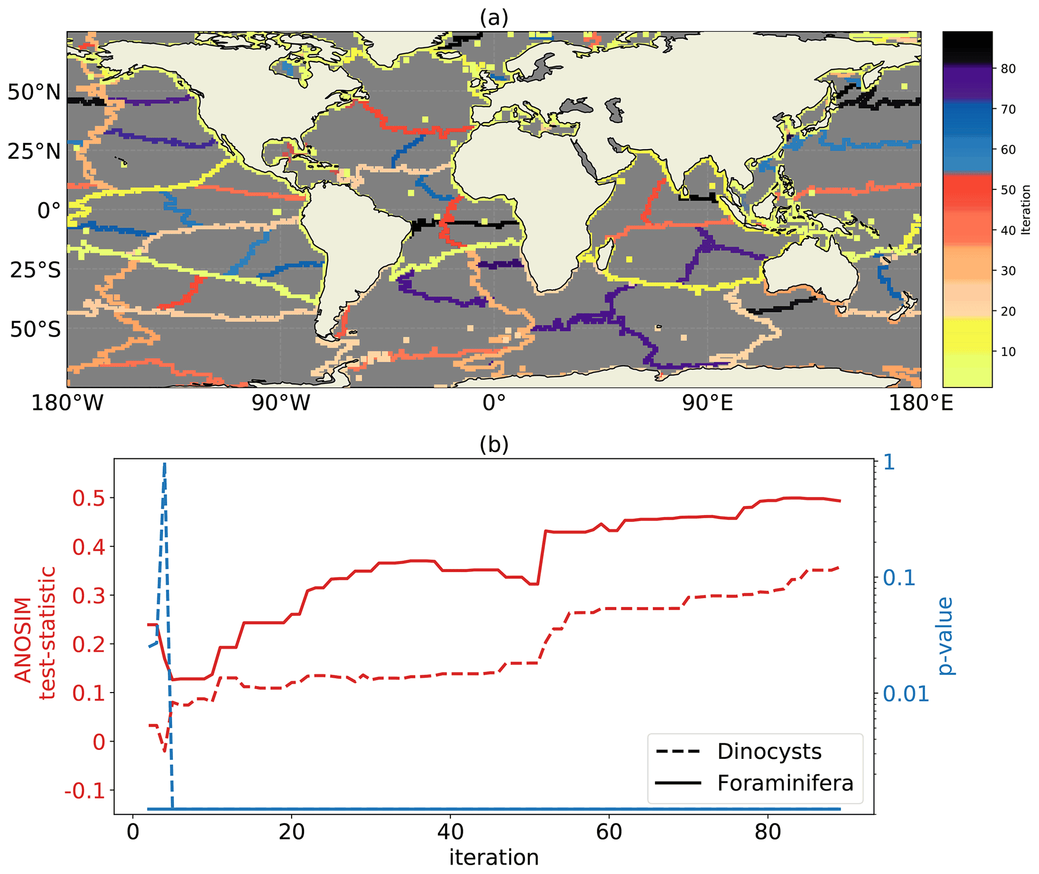
Figure 2 Edges between oceanographically disconnected clusters of sedimentary locations from the hierarchical clustering method. (a) The cluster edges after 90 iterations, where the colour indicates at which iteration number a cluster edge is created. (b) The ANOSIM test statistic (red) and p values (blue; 999 permutations; logarithmic scale) for the clusters at every iteration number, which tests whether the sedimentary microplankton composition (both dinocysts and foraminifera; sites below 65^∘ N) is more similar within than between clusters.

In the North Atlantic region, we observe that Hudson Bay becomes a cluster and the subtropical Atlantic is split from the Nordic Seas at the Greenland–Scotland ridge (Fratantoni, 2001; McClean et al., 2002; Bower et al., 2019). The Irminger Basin is still connected with the Labrador Sea, where sinking of water occurs (Pickart et al., 2003; Katsman et al., 2018), which makes transport of sinking particles outside of this area less likely. Only a few particles cross the connection between the Labrador Sea and Baffin Bay (McClean et al., 2002; Fischer et al., 2018).

We do not find a cluster at subpolar latitudes, which isolates Antarctica along latitudinal bands (only the Weddell and the Ross Sea are a cluster). One might expect such a cluster because near-surface currents are known to isolate Antarctica (Fraser et al., 2018; Dufour et al., 2015; Döös et al., 2008). However, deep passive particles advected by three-dimensional flow are shown to move upwards along isopycnals towards Antarctica (Drake et al., 2018; Tamsitt et al., 2018). As a result, the sinking particles can be transported towards Antarctica at depth. The location of southward particle transport is mainly determined by topographic steering of the flow, resulting in five hotspots of southward particle transport (Tamsitt et al., 2017) which roughly coincide with the Southern Ocean clusters in Fig. 2.

Some of the clusters in Fig. 2 are similar to connected regions based on the surface flow (see Fig. 8 from Froyland et al., 2014). The North and South Atlantic are split similarly from west Africa to Venezuela. The North Pacific and South Pacific are split in a similar way from Australia to the south of Chile. A cluster around the Pacific cold tongue (East Tropical Pacific) develops (Moum et al., 2013; Froyland et al., 2014). Moreover, the Benguela upwelling area (Nelson and Hutchings, 1983) (near south-west Africa) is more connected with the Southern Ocean than with the Atlantic. Near-surface currents have an important influence on the total lateral transport of sinking particles in these areas, since they are similar to the surface connectivity areas from Froyland et al. (2014).

We test whether sites within hierarchical clusters have a lower (Euclidean) taxonomic distance compared to sites of different clusters with analysis of similarities (ANOSIM; Clarke, 1993). The clustering corresponds to a high statistical significance for (1) positive ANOSIM test statistic together with (2) low p values (p value < 0.001). According to the ANOSIM tests, the clustering of sediment samples is significant across all iterations (Fig. 2c). Hence, sediment samples within clusters are more similar than those between clusters. The test statistic increases at higher iteration numbers, for both the dinoflagellate cyst (dinocyst) and the foraminifera dataset. Although these ANOSIM results look promising, it is important to note that the ANOSIM test statistics are partly positive because the sediment sites within clusters are closer to each other (i.e. there is a distance effect independent of the clustering).

The hierarchical clustering is overall insensitive to the sinking speed used of particles (see Figs. S1 and S2 in the Supplement with sinking speeds 11 and 25 m d⁻¹ respectively; see Appendix A1 for an explanation on why we did not test a sinking speed of 250 m d⁻¹). Only some minor differences occur in the North Pacific, and some cluster separations occur at slightly different iteration numbers. The fact that similar boundaries of little cross-transport emerge at a different sinking speed proves that the clustering does not greatly depend on the sinking speed of particles.

3.2 Oceanographically isolated clusters

The OPTICS clustering algorithm provides a density-based value (the reachability) of sedimentary sites, which quantifies how strongly a site is connected to other sites. Oceanographically isolated clusters can be obtained from the dense regions (i.e. areas with low reachability values), by setting a threshold on the slope that surrounds the dense values in the reachability plot (ξ). The sediment sites outside of these clusters are less isolated and referred to as noisy.

According to the OPTICS algorithm, the western boundary currents are unlikely to be part of any isolated cluster, since the points near the western boundary currents have a relatively high reachability (Fig. 3a). This is expected because the origin locations of sediment samples near western boundary currents comprise a large area. Dense areas are those at higher latitudes, close to Antarctica and in the Nordic Seas, and the midlatitude gyres. Sediment sample sites within these areas have more similar surface origin locations compared to sediment sites outside of dense areas. The high reachability values in the Mediterranean Sea and Red Sea are rather artificial. OPTICS searches for dense regions (low reachability) by searching for sedimentary sites with relatively many other sites having similar surface origin locations. Since the Mediterranean Sea and Red Sea are enclosed by land, these sedimentary sites have only few neighbouring sites, resulting in a relatively high reachability.

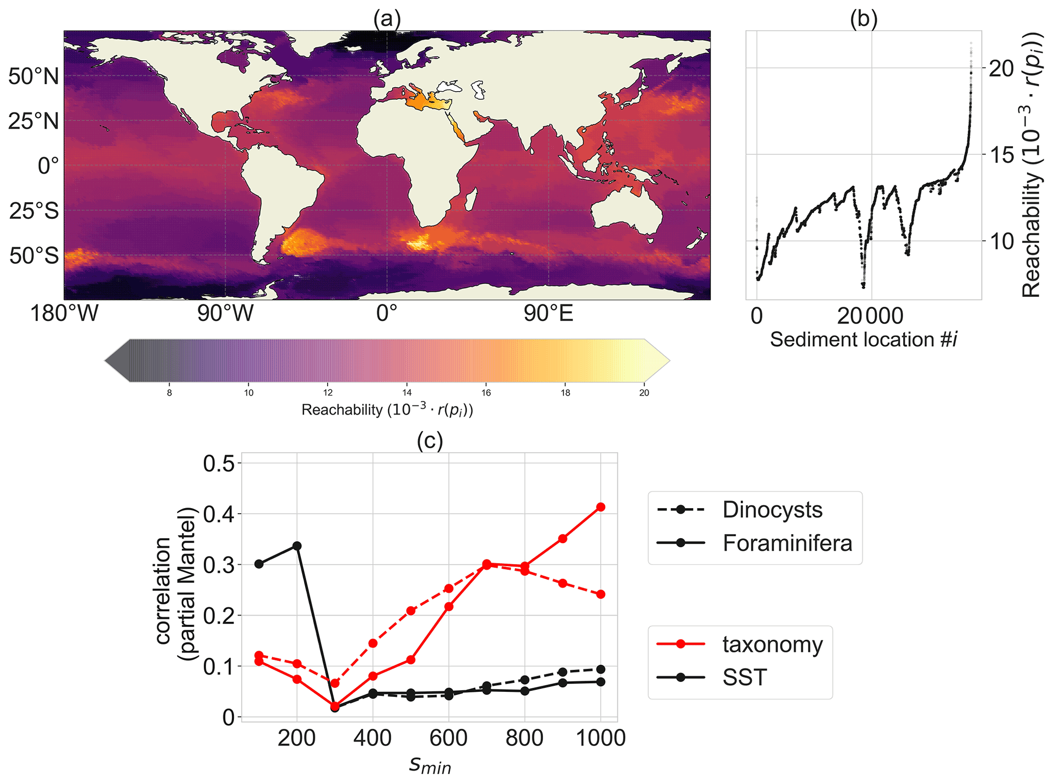
Figure 3 Reachability plot of the sedimentary particle release locations from the OPTICS algorithm. Sediment locations in dense areas (i.e. with low reachability values in a) share a similar particle distribution of backtracked surface origin locations, while areas with high reachability values have backtracked particle distribution which are more spread out and share origin locations with a lot of other sedimentary release locations. A sinking speed of 6 m d⁻¹ is used and parameter s_min=300 (i.e. OPTICS clusters will consist of a minimum of 300 sediment sites). (a) Site reachability in space: sites in dense areas with a low reachability are oceanographically isolated. (b) A scatter plot of the ordering of the sediment locations i against their reachability r(p_i). (c) Partial Mantel correlation of the reachability distance D^r (a lower value of D^r between two sites indicates a stronger oceanographic connection between these sites; see Appendix B) with the taxonomy (red) and SST (black), both with spatial distance held constant, for different s_min values. A total of 999 permutations were used for every partial Mantel test; every test with respect to the taxonomy (red) is significant with p value < 0.003.

The reachability distance (D^r; see Appendix B) between sediment sample sites correlates positively with sediment sample taxonomy. Furthermore, this correlation is independent of the spatial distance between sites, according to the partial Mantel tests (Legendre and Legendre, 2012) (Fig. 3c). This means that oceanographically connected sites have a similar taxonomy, independent of their spatial distance. Large values of s_min (>600; i.e. the OPTICS parameter which determines the minimum surface area in square metres of OPTICS clusters) tend to have the largest correlation (also at other sinking speeds; see Appendix B). This is probably because the reachability is smoother at higher s_min, which makes the reachability distance less noisy. At small spatial scales (s_min≤200), the correlation between dinocyst taxonomy and D^r could be indirect because then D^r correlates more strongly with the environment (in terms of sea surface temperature) compared to taxonomy.

We compute clusters by setting a threshold on the slope (ξ) that surrounds the reachability valleys in Fig. 3a. For ξ=0.002 and s_min=300 (Fig. 4), we obtain 13 clusters, of which three regions are isolated by the Antarctic Circumpolar Current (ACC), three in the Indian ocean, one in the Pacific warm pool, the South Atlantic gyre, near the Humboldt upwelling zone, near the Caribbean Sea, the eastern North Atlantic and two clusters near the Arctic. The clusters represent locations that are oceanographically isolated, with sediment sample sites that have backtracked origin locations which are similar to the other sites in the cluster. The environmental variability within these clusters can be reasonably large (e.g. the sea surface temperatures at backtracked origin locations in the cluster west of Australia range between 10–25 ^∘C; see https://planktondrift.science.uu.nl/, last access: 14 February 2022).

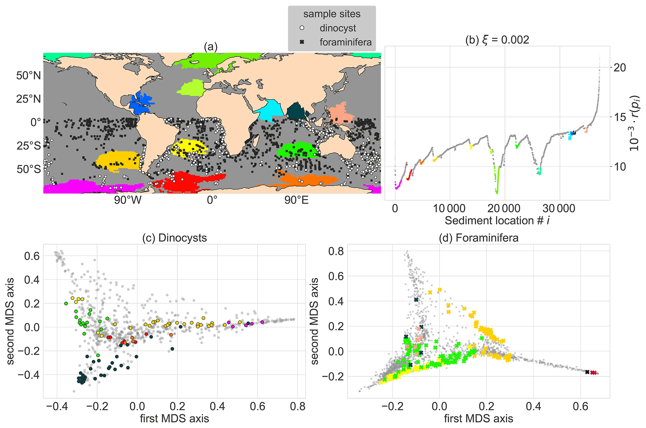
Figure 4 Oceanographically isolated OPTICS clusters of sedimentary particle release locations with clustering parameters s_min=300 (i.e. the minimum size of clusters) and ξ=0.002 (i.e. the level of isolation). The clustering is applied globally and the clusters are compared to Southern Hemisphere sediment sample sites. The coloured regions are clusters, the grey regions are “noisy” and therefore not part of a cluster. These colours were used for all subpanels. (a) Global map of the position of the clusters (coloured regions), and dinocyst (white) and foraminifera (black) sample locations. (b) Ordering of sedimentary locations i against their reachability r(p_i). To visualise the sediment sample site taxonomy for (c) the dinocysts and (d) the planktic foraminifera in two dimensions, we use classical multidimensional scaling (MDS; Fouss et al., 2016). MDS creates a two-dimensional approximation of the species composition in the sediment samples in this figure (instead of 91 and 50 dimensions or species for the dinocysts and foraminifera respectively).

The comparison between the clusters and taxonomic distance of Southern Hemisphere sample sites in these clusters (Fig. 4c and d) becomes interesting for clusters which are spatially close (Fig. 4b). For instance, the red and yellow clusters in the South Atlantic Ocean are spatially close, but sediment samples in those clusters are separated by their observed dinocyst taxonomy (Fig. 4c). This implies that we find a signal of the oceanographic separation of these areas in the sedimentary data. If noisy sites (such as the noisy site in Fig. 1b) were part of clusters, sites in different clusters are likely to contain a similar microplankton composition and the taxonomic separation of clusters is unclear.

To test if sedimentary sites within clusters are better correlated with environmental conditions at the surface, we applied CCA either including or excluding the sedimentary sites outside the isolated clusters (Fig. 5). We find that the amount of explained variation by the canonical axes increases significantly if noisy sediment samples are excluded for the foraminifera (∼0.92 to ∼0.95) and especially for the dinocysts (∼0.82 to ∼0.98), for the same OPTICS clusters as in Fig. 4. Hence, we find that the linear relationship between environmental variables and microplankton composition of the CCA explains a larger part of the sedimentary species composition if noisy sites are excluded. In that sense, the signal is “cleaner” for sediment sample sites within compared to outside clusters, which has implications for palaeoceanographic reconstructions of SST with these sedimentary data.

Figure 5 The relation between microplankton species variability and environmental variables according to a CCA analysis, while including and excluding unclustered sediment samples (using the isolated clusters from Fig. 4). Sea surface temperature (top) and nitrate concentration (bottom) at sediment sample sites with dinocysts (left; a–d) and foraminifera (right; e–h) against the first canonical axis from the CCA analysis, including (a, c, e, g) and excluding (b, d, f, h) sediment sample sites outside of the oceanographically isolated clusters. The sediment sample sites that belong to a cluster are coloured; “noisy” samples (i.e. not part of any cluster) are grey. The tables at the bottom show the proportion of total variance that is explained by the canonical axes if the noisy samples are included or excluded. Overall, 13.5 % (for dinocysts) and 10.8 % (for foraminifera) of the sediment sample sites is in clusters; the remainder is in noisy regions. The increase in explained variance is supported by a permutation test with 999 permutations (p values are <0.0001 and 0.024 for dinocysts and foraminifera respectively).

The robustness of the relationship between sedimentary sites and environmental variables is investigated by testing the sensitivity of the CCA results to these parameters ξ and s_min (Fig. 6). For the dinocyst dataset we find an increase in explained variation by the canonical axes for most tested values of s_min and ξ. By increasing the reachability slope that surrounds the oceanographically isolated clusters (ξ), a higher constraint is put on the isolation of these clusters and fewer sediment sample sites are part of a cluster. If this slope ξ is chosen too high, no clusters exist or they are too small to contain any sediment sample sites at all. Moreover, a higher value of ξ means that fewer sedimentary sites are used in the CCA (i.e. the dataset size is reduced), which may lead to an insignificant result according to the randomisation test. A relatively low value of ξ on the other hand may lead to insignificant results due to the inclusion of noisy sites in clusters. Hence, there seems to be an optimal value ξ, for which this increase in variance is maximised. These results are more often insignificant for the dinocysts compared to the foraminifera because the dinocyst dataset is smaller. If s_min is higher (i.e. the OPTICS algorithm finds larger clusters; in km²), the negative and insignificant values in Fig. 6 are partly caused by including noisy sites in clusters. These results highlight the importance of choosing an appropriate combination of ξ and s_min for the CCA to show a significant increased explained species variability if only clustered sites are used.

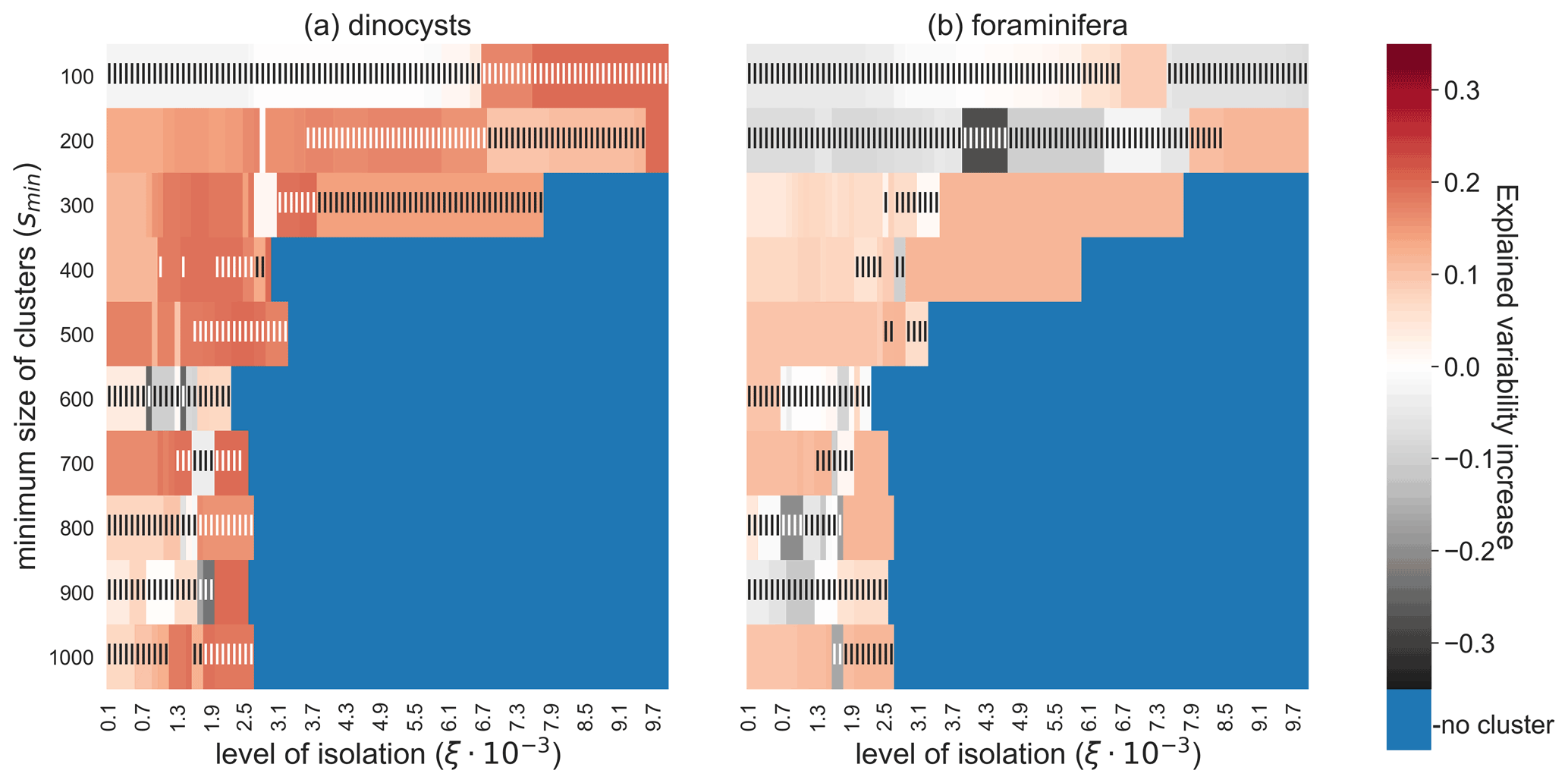
Figure 6 Increase in explained environmental variability by microplankton sediment sample sites in the CCA analyses if sediment samples outside of the oceanographically isolated OPTICS clusters are excluded, for different parameter values s_min (i.e. the minimum size of clusters) and ξ (i.e. the level of isolation). (a) The dinocyst and (b) the foraminifera dataset. High and significant values indicate that sediment samples within clusters have a clearer relationship with the surface environment. Blue are configurations of s_min and ξ for which no sediment sample sites are part of a cluster. Only Southern Hemisphere sedimentary microplankton data were used here. Vertical stripes indicate an insignificant randomisation test with 999 permutations at a 5 % significance level.

The clustered samples are less taxonomically mixed (i.e. are less biodiverse) for most values of ξ and s_min, as we can see from the comparison between the Shannon entropy (N_s; see the Method section) within and outside of clusters (Fig. 7). For the high values of s_min, we find that the clusters are less taxonomically mixed if ξ is increased. This result supports that measured microplankton biodiversity in sediments is relatively large in areas with strong mixing of sinking particles by ocean currents. However, the Shannon entropy is also influenced by the species distributions at the ocean surface, for which much fewer species composition data are available compared to their sedimentary remains. At smaller values of s_min (s_min<200 and s_min<300 for the dinocysts and foraminifera respectively; Fig. 7) high (surface) productivity areas are also clustered (e.g. the south-west Atlantic or the Humboldt area; see Fig. 4). Hence, a relatively high sedimentary biodiversity in these clusters can be explained by the high biodiversity at the ocean surface, before these particles start sinking.

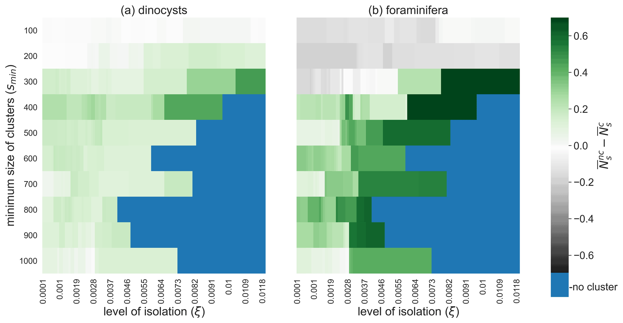
Figure 7 Sedimentary microplankton biodiversity outside minus inside oceanographically isolated provinces. The average Shannon entropy of (a) dinocysts and (b) foraminifera sediment samples inside OPTICS clusters ${\stackrel{\mathrm{‾}}{N}}_{\mathrm{s}}^{\mathrm{c}}$ compared to outside clusters ${\stackrel{\mathrm{‾}}{N}}_{\mathrm{s}}^{\mathrm{nc}}$ for different values of s_min (i.e. the minimum size of clusters) and ξ (i.e. the level of isolation). High values indicate that the number of species in samples within clusters are lower and species are distributed less evenly in samples compared to samples outside clusters. Blue are configurations of s_min and ξ for which no sediment sample sites are part of a cluster.

We also tested the OPTICS results for sinking velocities higher than 6 m d⁻¹ (11, 25, and 250 m d⁻¹; see Figs. S5–S10 and S11–S14). Similar clusters can be found with the other sinking velocities. A higher sinking speed decreases the particle travel time; thus the lateral transport and the mixing of sinking particles is overall lower (Nooteboom et al., 2019). However, the spatial dependence of the lateral transport is similar: both at low and high sinking velocities, the lateral particle transport is relatively large near western boundary currents and low in the middle of midlatitude gyres (Nooteboom et al., 2020). As a result, the clusters are located in similar areas for different sinking speeds. It is only the spatial scale of these clusters that might be different. The spatial scale (i.e. the size) of the clusters can again be controlled by the parameters s_min and ξ. Note that high-productivity areas are less likely clustered at higher sinking speeds, which has implications for the Shannon entropy within and outside clusters (Fig. 7): higher biodiversity is measured outside compared to within clusters for a larger area of s_min and ξ values as the sinking speed increases.

4 Discussion

We clustered sediment sites based on the ocean surface origin locations of sinking particles that end up at these sites in an ocean model. These clusters reveal which sedimentary areas are oceanographically (1) (dis)connected or (2) isolated. The connectivity which is given by the clusters is an aggregate of the ocean connectivity at all depths that the sinking particles traverse before ending up in the sediments. This type of connectivity, and the way it shapes the sedimentary microplankton composition, is additive to the environment and surface ocean connectivity which influences the plankton community structure at the ocean surface (Jonnson and Watson, 2016; Wilkins et al., 2013). Nevertheless, the near-surface flow likely has a large imprint on the clusters since these contain the strongest ocean currents.

It was shown before that the ocean surface ecological affinity of certain sedimentary microplankton species can improve if the lateral advection of sinking particles is taken into account (Nooteboom et al., 2019). This paper explores reasons why sedimentary plankton assemblages include species that occur outside their surface water habitat range. Microplankton species mix by turbulent ocean currents during their sinking journey, which can result in a relevant lateral displacement along transport. The extent by which this occurs differs strongly in the world oceans and is larger in areas that are referred to as noisy in this paper.

We conclude that ocean sediments are to a spatially varying degree provincial, and province boundaries are governed by near-surface and deep currents in the ocean. These provinces have implications for sedimentary microplankton assemblages. Their quantification helps to determine ocean sediment regions that are oceanographically (a) (dis)connected and (b) isolated from the area outside of these regions. Quantification of connected and isolated provinces has at least four implications for future studies.

First, the clustering methods that are presented in this paper can help to improve the application of transfer functions on microplankton assemblages. Transfer functions train a model on surface sediment samples and ocean surface environmental variables (in the present day), in order to make quantitative climate reconstructions of past climates from microplankton in deeper sediments. Hence, these transfer function models use spatial variability of an environmental variable to predict its temporal variability in a single location. One challenge of transfer functions is to choose a proper spatial extent to train the prediction model (Hohmann et al., 2019; often in the present-day situation). A small spatial extent does not capture enough of species and environment variability. If the spatial extent is too large, different processes determine the sedimentary species distribution which reduces the transfer function skill.

The hierarchical clustering method (which finds oceanographically disconnected clusters) can help to determine bounds on the spatial extent that is used for the training of transfer functions (e.g. a transfer function can be trained on sites within a single cluster), since it shows areas which are oceanographically separated from each other. These clusters are created in a present-day configuration in this study and may change in past climates. The OPTICS clustering can be used to find oceanographically isolated clusters to determine the spatial extent of a regional transfer function model. In this case, it is advisable to check if the OPTICS cluster is large enough (i.e. the deep sediments do not contain species outside of the cluster).

Second, the connectivity between provinces could have an effect on biogeochemical properties of microplankton species that are applied as a proxy of the ocean surface environment. These provinces can be used to correct for ocean connectivity by providing a different reference frame (Weyl, 1978) if the proxies are used to assimilate, e.g., global sea surface temperature fields (as in Tierney et al., 2020). This may require the computation of these clusters using palaeoceanographic models. Moreover, spatially varying Bayesian regression is used to some of these biogeochemical proxies because the proxy response differs across oceanic basins (Tierney and Tingley, 2015, 2018). Since proxy calibration residuals are often high in specific areas and related to lateral advection (Tierney and Tingley, 2018), the (dis)connected provinces from this paper can provide a spatial structure that such a regression model uses for core-top calibration.

Third, the results in this paper have implications for other types of sinking particles in the ocean. For instance, a large fraction of marine plastic sinks to the ocean floor (Canals et al., 2020; Kooi et al., 2017). Sedimentary plastic distributions might be subject to similar mechanisms of mixing during their sinking journey. Clustering of sedimentary sites might indicate where the largest inhomogeneities of sedimentary plastics appear (de la Fuente et al., 2021) or boundaries where sinking plastic is less likely to cross.

Fourth, our study provides micropalaeontologists with a tool to qualitatively assess the importance of lateral transport to sedimentary particle assemblages, which can be used in studies that compare measured biological diversity and environmental conditions in surface waters with their sedimentary remains (e.g. Jonkers et al., 2019; Meilland et al., 2020), particularly in those regions for which we here demonstrate noisy behaviour: within oceanographically isolated clusters, sedimentary microplankton biodiversity is only weakly determined by lateral particle transport compared to the microplankton biodiversity near the ocean surface and species-specific dissolution (Frenger et al., 2018; Taylor et al., 2018).

Drivers of biodiversity at the ocean surface, such as species interactions (Lima-Mendez et al., 2015), ecological limits and evolutionary dynamics (Fenton et al., 2016), are complex. It is possible that oceanographically isolated provinces do not directly drive a low biodiversity but indirectly cause a low biodiversity through a lower variation in abiotic factors. Moreover, these provinces are likely located in areas with relatively little eddy activity, while mesoscale eddies can explain relatively high biodiversity values (Frenger et al., 2018).

The backtracking analysis on which we applied the clustering was designed for dinocysts and not for foraminifera. In particular, near-surface advection during the foraminifera lifespan may have a larger impact on its sedimentary distribution compared to the lateral transport during sinking (Ottens and Nederbragt, 1992). Clustering results from this paper compared well with the foraminifera dataset in most cases because the areas with strong particle mixing and lateral transport (i.e. their spatial dependence) are likely similar for foraminifera (and likely similar at the near-surface compared to other depth levels). Nevertheless, future work could apply these clustering methods on a backtracking analysis which is designed for foraminifera (similar to van Sebille et al., 2015a; Lange and Sebille, 2017). This means that particles are released at the ocean bottom, tracked back in time until they reach the foraminifera dwelling depth, and finally tracked back during their lifespan at this dwelling depth.

Appendix A: Clustering methods

A1 Hierarchical clustering

The particle tracking results from Nooteboom et al. (2019) can be described by a bipartite graph (or transportation matrix; Fig. A1a). This bipartite graph consists of bottom and surface nodes (representative of surface and bottom boxes in the transportation matrix; we use $\mathrm{1}{}^{\circ }\times \mathrm{1}{}^{\circ }$ boxes in this paper). Bottom and surface nodes are linked if the probability that a particle which is found in a bottom box originates from the surface box is greater than zero. We will use the projection of this bipartite graph on the bottom nodes (Fig. 1c). This provides us with a graph of only bottom nodes, where the weight of a link between two nodes is determined by the number of common surface nodes they are linked to in the bipartite graph.

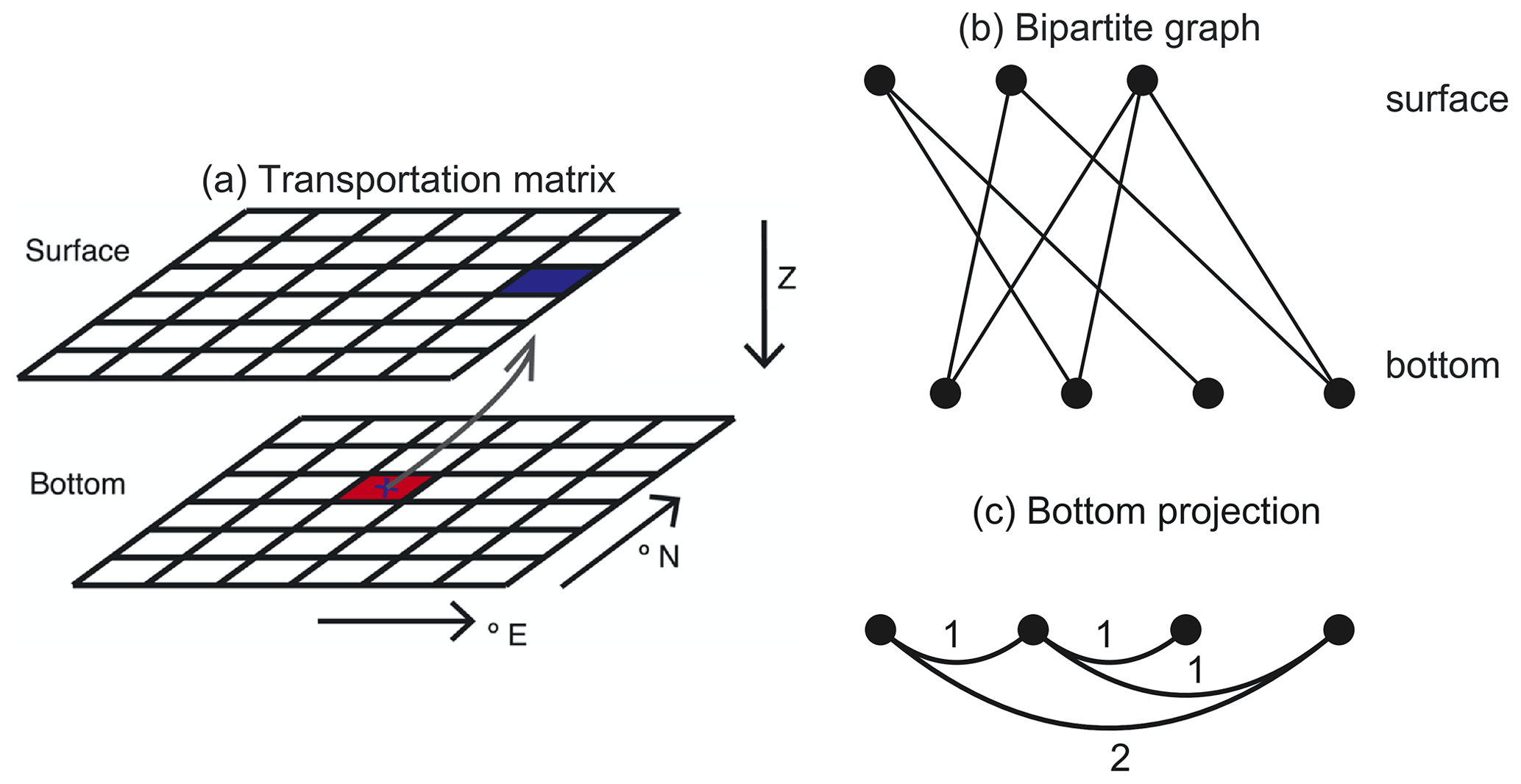
Figure A1 Illustrations for the embedding types that the hierarchical clustering method uses. (a) Illustration of the surface-bottom transportation matrix (figure adapted from Nooteboom et al., 2019). The transportation matrix contains the probabilities that a particle that is found in a bottom box originated from a surface box. The transportation matrix can also be interpreted as a bipartite graph in (b), which has a bottom projection (c): the bottom nodes are linked with a weight that is determined by the number of mutually linked surface vertices in the bipartite graph.

Given the projection of the bipartite graph on the bottom nodes, we apply the hierarchical clustering method as described in Wichmann et al. (2020). Starting with the largest connected component in the bottom projection as the only cluster (which represents the full global ocean), the clustering algorithm chooses one cluster at every iteration and splits it into two clusters, such that the normalised cut (NCut) is minimised (Shi and Jitendra, 2000). For K clusters $S_{\mathrm{1}},\mathrm{\cdots },S_K$, the NCut is defined as

$$\begin{array}{}\text{(A1)}& \mathrm{NCut}\left(S_{\mathrm{1}},\mathrm{\cdots },S_K\right):=\sum _{i=\mathrm{1}}^K{\displaystyle \frac{Q\left(S_i,S_i^{\mathrm{C}}\right)}{Q\left(S_i,S\right)}},\end{array}$$

where Q(S_i,S_j) is the sum of all weights connecting S_i and S_j, $S_i^{\mathrm{C}}$ is the complement of S_i. By definition, the NCut increases at every iteration (i.e. if the number of clusters is higher).

We do not test the hierarchical clustering at 250 m d⁻¹ sinking speed of particles in the backtracking analysis. The particle distributions spread less at this sinking velocity, and the bottom projection of the bipartite graph becomes disconnected. Hence, these higher sinking speeds require a higher resolution binning of the input used, which exceeds given computational limitations.

A2 OPTICS clustering

We use OPTICS to compare clusters with the sediment sample sites, which is density-based and distinguishes different clusters from “noise” (Wichmann et al., 2020). We apply OPTICS in this paper to the “direct embedding” of surface origin distributions (Fig. 1a).

The main result from OPTICS is the reachability plot (see Wichmann et al., 2021, for more details). The reachability plot is a representation of the global and local distribution of points (which represent sedimentary sites in this paper) at once. The valleys correspond to dense regions with similar surface origin location, while the hills correspond to the noisy locations. The reachability plot depends on a parameter s_min, for which we test multiple values ($s_{\min }\in [\mathrm{100},\mathrm{200},\mathrm{300},\mathrm{400},\mathrm{500},\mathrm{600},\mathrm{700},\mathrm{800},\mathrm{900},\mathrm{1000}]$). s_min sets the minimum number of “nearby” points in the reachability plot for every point in a cluster (MinPts in Ester et al., 1996). In general, a larger s_min results in a smoother reachability plot and larger clusters. If we let every particle release location (released on a $\mathrm{1}{}^{\circ }\times \mathrm{1}{}^{\circ }$ grid) represent an area of 1^∘ (∼10⁴ km²), the OPTICS algorithm searches for a cluster with a spatial scale $\sim s_{\min }\times {\mathrm{10}}^{\mathrm{4}}$ km².

In this paper, we use ξ clustering to obtain clusters from the reachability plot (Ankerst et al., 1999). This implies that we set a threshold on the steepness of the density (ξ) and cluster the valley of points that is surrounded by this steepness ξ. In general, a larger ξ will reduce both the size and the number of clusters.

Appendix B: The distance matrices defined

We use (symmetric) distance matrices based on four different metrics. First, we use a matrix that contains Euclidean taxonomic distances, calculated from the relative abundances (fractions) of species. Second, we use the absolute SST differences between the sites. Third, we use a distance which is based on the reachability from the OPTICS algorithm. Specifically, if r(p_k) is the reachability of point p_k and the n points are ordered from p₀ ⋯ p_n, the reachability distance between two sediment sample sites (located near p_i and p_j respectively with i≤j) is $D_{ji}^{\mathrm{r}}=D_{ij}^{\mathrm{r}}={\max }_{i\le k\le j}r\left(p_k\right)-{\min }_{i\le k\le j}r\left(p_k\right)$. Intuitively, $D_{ij}^{\mathrm{r}}$ represents how much one has to climb or descend in the reachability “landscape” if one likes to move from point i to j. Fourth, we use a distance matrix which contains the spatial distance (in metres) between sediment sample sites. The partial Mantel test determines the correlation between the reachability distance and either SST or taxonomy distance matrices, keeping the spatial distance matrix constant.