the Creative Commons Attribution 4.0 License.
the Creative Commons Attribution 4.0 License.
 | 25 Jan 2022
Oceanographic regional climate projections for the Baltic Sea until 2100
H. E. Markus Meier
Christian Dieterich
Matthias Gröger
Cyril Dutheil
Florian Börgel
Kseniia Safonova
Ole B. Christensen
Erik Kjellström
The Baltic Sea, located in northern Europe, is a semi-enclosed, shallow and tideless sea with seasonal sea-ice cover in its northern sub-basins. Its long water residence time contributes to oxygen depletion in the bottom water of its southern sub-basins. In this study, recently performed scenario simulations for the Baltic Sea including marine biogeochemistry were analysed and compared with earlier published projections. Specifically, dynamical downscaling using a regionally coupled atmosphere–ocean climate model was used to regionalise four global Earth system models. However, as the regional climate model does not include components representing terrestrial and marine biogeochemistry, an additional catchment and a coupled physical–biogeochemical model for the Baltic Sea were included. The scenario simulations take the impact of various global sea level rise scenarios into account. According to the projections, compared to the present climate, higher water temperatures, a shallower mixed layer with a sharper thermocline during summer, less sea-ice cover and greater mixing in the northern Baltic Sea during winter can be expected. Both the frequency and the duration of marine heat waves will increase significantly, in particular in the coastal zone of the southern Baltic Sea (except in regions with frequent upwellings). Nonetheless, due to the uncertainties in the projections regarding regional winds, the water cycle and the global sea level rise, robust and statistically significant salinity changes could not be identified. The impact of a changing climate on biogeochemical cycling is predicted to be considerable but still smaller than that of plausible nutrient input changes. Implementing the proposed Baltic Sea Action Plan, a nutrient input abatement plan for the entire catchment area, would result in a significantly improved ecological status of the Baltic Sea, including reductions in the size of the hypoxic area also in a future climate, which in turn would increase the resilience of the Baltic Sea against anticipated climate change. While our findings regarding changes in heat-cycle variables mainly confirm earlier scenario simulations, they differ substantially from earlier projections of salinity and biogeochemical cycles, due to differences in experimental setups and in input scenarios for bioavailable nutrients.


The Baltic Sea is a shallow, semi-enclosed sea located in northern Europe (Fig. 1). It has a mean depth of 54 m, but due to its strongly varying bottom topography it can be divided into several sub-basins, with limited transport between them (Sjöberg, 1992). In particular, water exchange between the Baltic Sea and the North Sea is hampered because of two shallow sills located in narrow channels connecting these two water bodies. Thus, large saltwater inflows occur only sporadically, on average once per year, mainly during the winter season but never during summer (Mohrholz, 2018). Furthermore, because the Baltic Sea is embedded within a catchment area that is about 4 times larger than the Baltic Sea surface, annual freshwater inputs are large relative to the volume of the Baltic Sea (Bergström and Carlsson, 1994). The volume of the Baltic Sea is ∼21 700 km3 (Sjöberg, 1992) and the turnover time of the total freshwater supply (∼16 000 m3 s−1) is 35 years (Meier and Kauker, 2003). These features contribute to strong horizontal and vertical salinity gradients in the Baltic Sea (Fonselius and Valderrama, 2003). Moreover, due to its location and physical characteristics, especially the long water residence time, the Baltic Sea is vulnerable to external pressures, including eutrophication, pollution and global warming (e.g. Jutterström et al., 2014). Ocean circulation modelling has shown that the timescale of the salinity response to changes in atmospheric and hydrological forcing is 20 years (Meier, 2006).
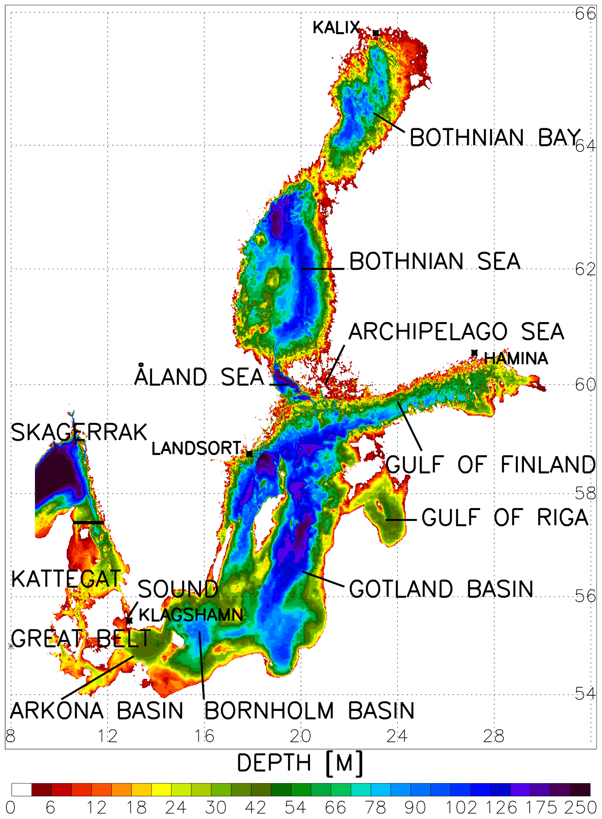
Figure 1Bottom topography of the Baltic Sea (depth in metres). The Baltic Proper comprises the Arkona Basin, Bornholm Basin and Gotland Basin. The border of the analysed domain of the Baltic Sea models is shown as a black line in the northern Kattegat. The tide gauges in Klagshamn (55.522∘ N, 12.894∘ E), Landsort (58.742∘ N, 17.865∘ E), Hamina (60.563∘ N, 27.179∘ E) and Kalix (65.697∘ N, 23.096∘ E) are also depicted.
Some 85 million people, in 14 countries, currently live in the catchment area of the Baltic Sea, and anthropogenic pressure on the marine ecosystem is accordingly high (HELCOM, 2018). Insufficiently treated wastewater, pollutant emissions, overfishing, habitat degradation and intensive marine traffic, including oil transport, place a heavy burden on the Baltic Sea ecosystem (Reckermann et al., 2022). One consequence is oxygen depletion of the Baltic Sea's deep waters, such that bottom areas lack higher life forms (e.g. Carstensen et al., 2014; Meier et al., 2018b). In 2018, the area of dead bottom was equal to that of the Republic of Ireland, ∼73 000 km2, which is about one-fifth of the sea surface area of the Baltic Sea (without the Kattegat). Oxygen depletion in the deeper parts of the Baltic Sea arises from the limited ventilation of those waters and the accelerated oxygen consumption that accompanies the remineralisation of organic matter (Meier et al., 2018b). Hence, nutrient input abatement strategies, such as the Baltic Sea Action Plan (BSAP), have been proposed (HELCOM, 2007), with projections of their impact requested by stakeholders such as the Helsinki Commission (HELCOM) or national environmental protection agencies1.
Table 1Selected ensembles of the scenario simulations for the Baltic Sea carried out in international projects (AR is the IPCC Assessment Report, GCM is a general circulation model, RCSM is a regional climate system model, RCAO is the Rossby Centre Atmosphere Ocean model, RCA4 is the Rossby Centre Atmosphere model version 4, NEMO is the Nucleus for European Modelling of the Ocean, REMO is a regional model, MPIOM is the Max Planck Institute Ocean Model, and HAMSOM is the Hamburg Shelf Ocean Model).
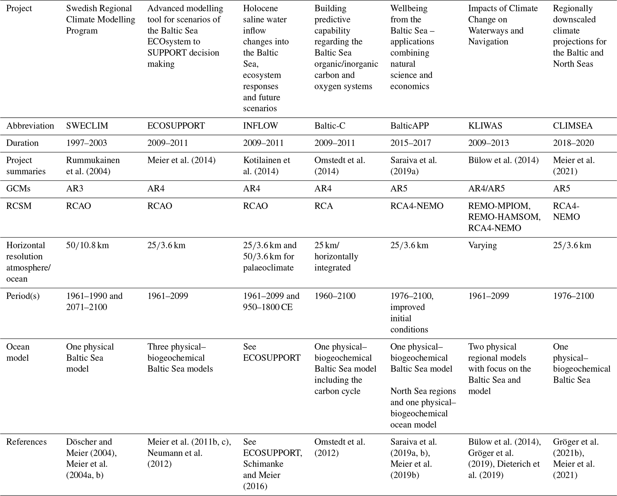
Projections of the Baltic Sea's climate at the end of the 21st century were among the first to be made for coastal seas worldwide (Meier and Saraiva, 2020). Already at the beginning of the 2000s, the first scenario simulations were carried out for selected time slices in present and future climates (e.g. Haapala et al., 2001; Meier, 2002a, b; Omstedt et al., 2000). In the dynamical downscaling approach used for those simulations, regional climate models (RCMs) were employed to refine predictions of global climate change to regional and local scales, in this case for the Baltic Sea (e.g. Rummukainen et al., 2004; Döscher et al., 2002). However, those first projections were based on scenarios consisting of a single global climate model (GCM) and a single greenhouse gas (GHG) concentration (150 % increase in equivalent CO2 concentration in the atmosphere in the future vs. the historical climate) and only covered 10-year time slices. These initial attempts were therefore followed by more advanced scenario simulations using mini-ensembles (e.g. Döscher and Meier, 2004; Meier et al., 2004a, b; Räisänen et al., 2004) and centennial-long simulations (e.g. Meier, 2006; Meier et al., 2006, 2011c; Table 1). However, the latter studies considered only monthly mean changes in the future vs. the present climate, applying a so-called delta approach, while neglecting possible changes in interannual variability. From these oceanographic studies it was concluded that “mean annual sea surface temperatures (SSTs) could increase by some 2 to 4 ∘C by the end of the 21st century. Ice extent in the sea would then decrease by some 50 % to 80 %. The average salinity of the Baltic Sea could range between present day values and decreases of as much as 45 %. However, it should be noted that these oceanographic findings, with the exception of salinity, are based upon only four regional scenario simulations using two emissions scenarios and two global models” (BACC Author Team, 2008).
For the second assessment of climate change in the Baltic Sea region (BACC II Author Team, 2015), continuously integrated transient simulations from present to future climates became available and even included marine biogeochemical modules (e.g. Eilola et al., 2013; Friedland et al., 2012; Gräwe and Burchard, 2012; Gräwe et al., 2013; Gröger et al., 2019, 2021b; Holt et al., 2016; Kuznetsov and Neumann, 2013; Meier et al., 2011b, c, 2012a, c, d; Neumann, 2010; Neumann et al., 2012; Omstedt et al., 2012; Pushpadas et al., 2015; Ryabchenko et al., 2016; Skogen et al., 2014) and higher trophic levels (e.g. Bauer et al., 2019; Ehrnsten et al., 2020; Gogina et al., 2020; Holopainen et al., 2016; MacKenzie et al., 2012; Niiranen et al., 2013; Vuorinen et al., 2015; Weigel et al., 2015). The BACC II Author Team (2015) concluded that “recent studies confirm the findings of the first assessment of climate change in the Baltic Sea basin”. A key finding of their report was that “No clear tendencies in saltwater transport were found. However, the uncertainty in salinity projections is likely to be large due to biases in atmospheric and hydrological models. Although wind speed is projected to increase over sea, especially over areas with diminishing ice cover, no significant trend was found in potential energy …” (a measure of energy to homogenise the water column). “In accordance with earlier results, it was found that sea level rise has greater potential to increase surge levels in the Baltic Sea than does increased wind speed. In contrast to the first BACC assessment (BACC Author Team, 2008), the findings reported in this chapter are based on multi-model ensemble scenario simulations using several GHG emissions scenarios and Baltic Sea models. However, it is very likely that estimates of uncertainty caused by biases in GCMs are still underestimated in most studies” (BACC II Author Team, 2015).
Since the early 21st century, transient simulations for the period 1960–2100 using regional ocean (Holt et al., 2016; Pushpadas et al., 2015) and regionally coupled atmosphere–ocean models, so-called regional climate system models (RCSMs; Bülow et al., 2014; Dieterich et al., 2019; Gröger et al., 2019, 2021b), have been available for the entire combined Baltic Sea and North Sea system. An overview was given by Schrum et al. (2016) as part of the North Sea Region Climate Change Assessment Report (NOSCCA, Quante and Colijn, 2016) and by Gröger et al. (2021a) within the Baltic Earth Assessment Reports (BEAR) project (this thematic issue).
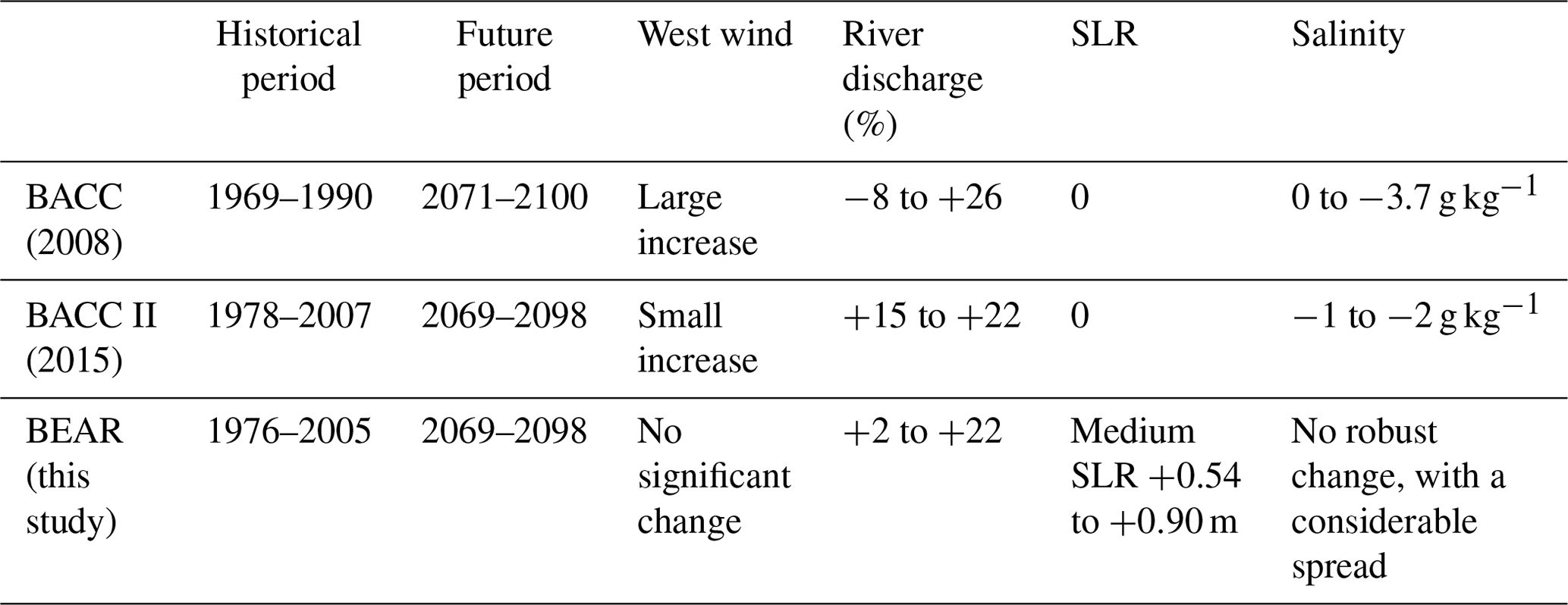
There is a notable difference in the salinity projections between the first two assessments (BACC Author Team, 2008; BACC II Author Team, 2015) and recent scenario simulations (Meier et al., 2021). The first Baltic Sea scenario simulations, driven by nine RCMs and five GCMs, showed a pronounced negative ensemble mean change in salinity because two of the GCMs included a significant increase in the mean west wind component (Meier et al., 2006). These pronounced changes in the large-scale atmospheric circulation were not a feature of later studies (Saraiva et al., 2019a). However, as the natural variability was poorly sampled, this finding may be coincidental.
The large spread in river discharge did not decrease between the studies, ranging from −8 % to +26 % (Meier et al., 2006, 2021). Since in more recent assessments the projected rates of global sea level rise (SLR) were revised upwards (e.g. IPCC, 2019a; Bamber et al., 2019), recent scenario simulations for the Baltic Sea also considered a rise in sea level (Meier et al., 2021). As a consequence of compensating effects of the competing drivers of salinity changes, i.e. wind, freshwater input and sea level, future salinity changes were predicted to be small (Table 2).
Table 2Salinity projections assessed by the BACC Author Team (2008), BACC II Author Team (2015) and BEAR (this study). Salinity changes depend on the changes in the wind field (in particular, the west wind component), river discharge and sea level rise (SLR). The changes refer to the mean differences between historical and future periods. (Data sources: Meier et al., 2006, 2011b, 2021).
In the following, we provide an overview of the projections performed since 2013, i.e. after the last assessment of climate change for the Baltic Sea basin, and compare recent results with previous findings by the BACC II Author Team (2015). We focus on projections for the marine environment from both physical and biogeochemical perspectives. Among the analysed variables are temperature, salinity, oxygen, phosphate, nitrate, phytoplankton, primary production, nitrogen fixation, hypoxic area and Secchi depth (measuring water transparency). An accompanying study by Christensen et al. (2021) investigated atmospheric projections in the Baltic Sea region. For an overview of the development of RCSMs and their applications, the reader is referred to Gröger et al. (2021a). In our comparisons of the various scenario simulations, we analyse only published data (Table 1), with a focus on two recently generated sets of scenario simulations: BalticAPP and CLIMSEA (Table 1; see Saraiva et al., 2019a, b; Meier et al., 2019a, 2021). These are compared with the previous ECOSUPPORT scenario simulations (Meier et al., 2014) assessed by the BACC II Author Team (2015). Investigations of the impact of climate change on primary production in the Baltic Sea that did not utilise a RCM (Holt et al., 2016; Pushpadas et al., 2015) are not addressed herein, nor are nutrient input reduction scenarios under present climate, e.g. as described by Friedland et al. (2021). To our knowledge, further coordinated experiments aimed at projections for the coupled physical–biogeochemical system of the Baltic Sea after 2013 have not been published. Uncoordinated scenario simulations performed prior to 2013 (including Ryabchenko et al., 2016) and their uncertainties were previously discussed by Meier et al. (2018a, 2019b).
The paper is organised as follows. In Sect. 2, the dynamical downscaling method, the catchment and Baltic Sea models, the experimental setup and the analytical strategy are introduced. In Sect. 3, the historical and future climates results of the three scenario simulations, ECOSUPPORT, BalticAPP and CLIMSEA, are compared. Tables 1, 3 and 4 provide an overview of these (Tables 3 and 4) and other (Table 1) scenario simulations from the literature. A consideration of knowledge gaps and a summary of our findings conclude the study. Abbreviations used in this study are defined in Table 5.
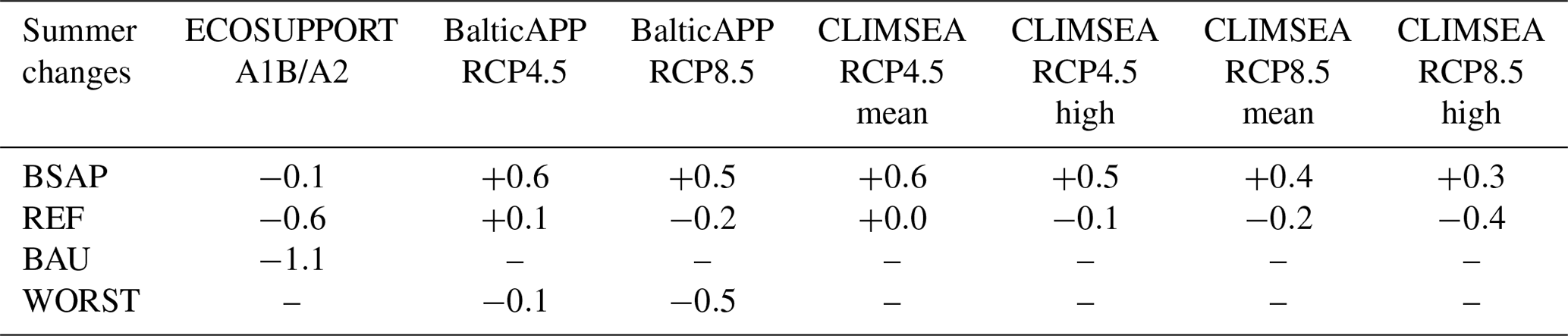
Table 3List of scenario simulations of three ensembles. From left to right, the columns show the Earth system model (ESM), the regional climate system model (RCSM), the Baltic Sea ecosystem model, the greenhouse gas (GHG) emission or concentration scenario, the nutrient input scenario, the sea level rise (SLR) scenario and the simulation period, including historical and scenario periods. The four nutrient input scenarios were the Baltic Sea Action Plan (BSAP), reference (REF), business-as-usual (BAU) and worst case (WORST) scenarios. For the three SLR scenarios in the CLIMSEA ensemble, the mean sea level changes at the end of the century are given in metres.
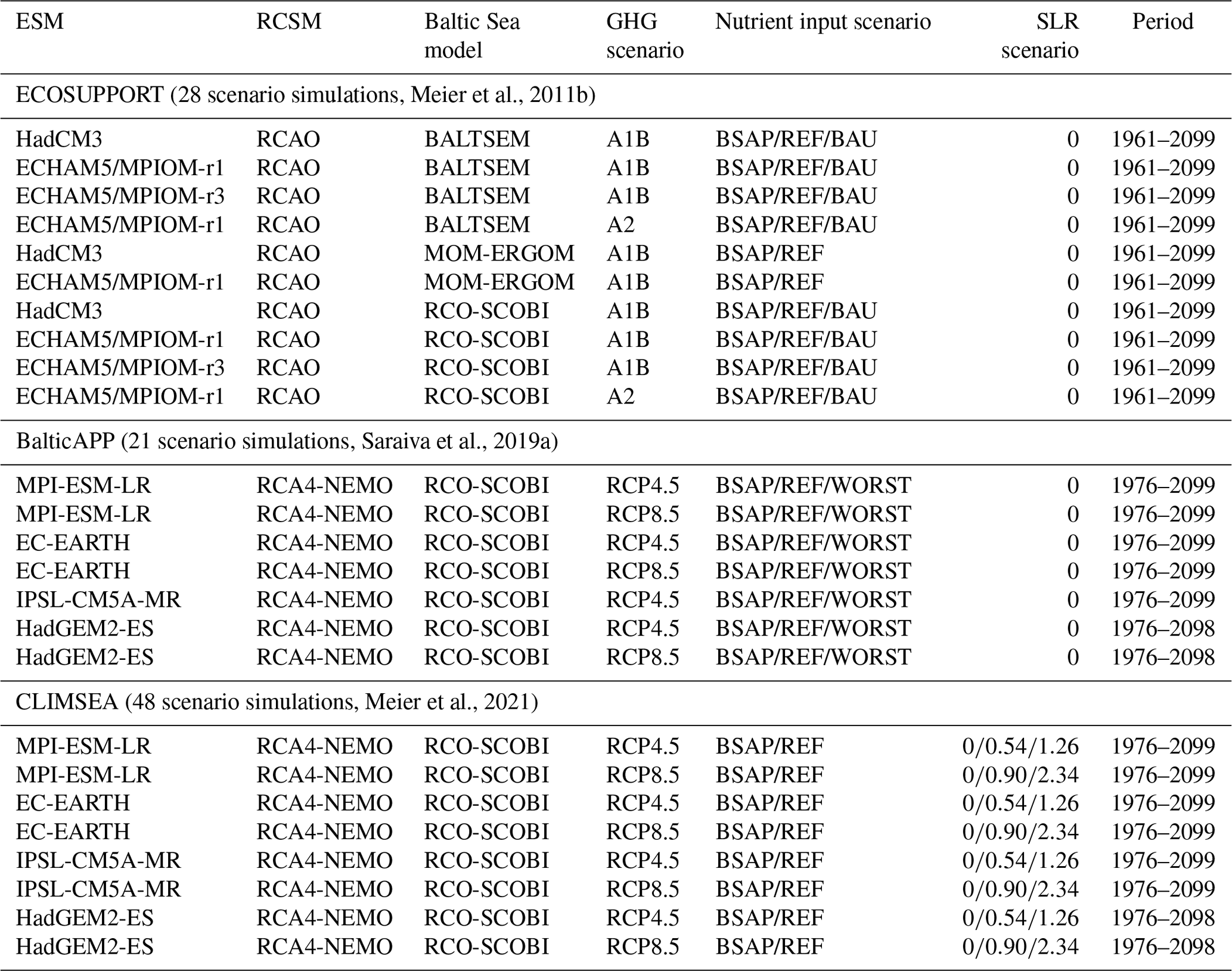
Table 4Summary of the characteristics of the ECOSUPPORT, BalticAPP and CLIMSEA scenario simulations discussed in this study. For further details, the reader is referred to Tables 1 and 3. Abbreviations are defined in Table 5.
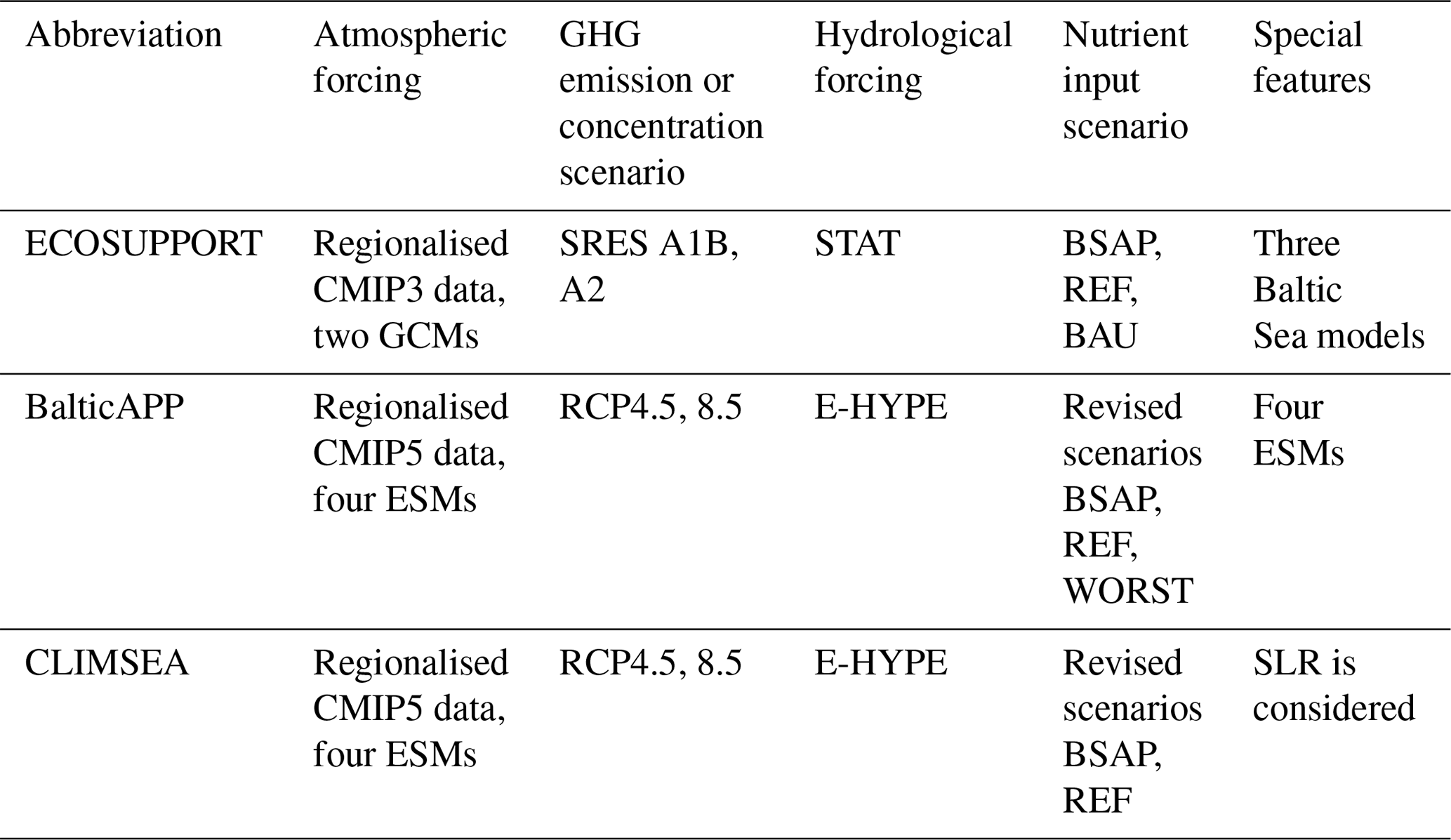
Table 5List of abbreviations (in alphabetical order), their definitions and references.

2.1 Regionalisation of a changing climate
Dieterich et al. (2019) produced an ensemble of scenario simulations with a coupled RCSM, called RCA4-NEMO, which was introduced by Wang et al. (2015). Gröger et al. (2019, 2021b) and Dieterich et al. (2019) validated and analysed the different aspects of the RCA4-NEMO ensemble discussed herein. The atmospheric component, RCA4 (Rossby Centre Atmosphere model version 4), was run at a resolution of 0.22∘ and 40 vertical levels in the EURO-CORDEX domain (Jacob et al., 2014), and the coupled North Sea–Baltic Sea model NEMO (Nucleus for European Modelling of the Ocean) at a resolution of 2 nautical miles (3.7 km) and 56 levels. The two components of the RCSM are coupled by sending sea surface data of sea level pressure, energy, mass and momentum fluxes every 3 h from the atmosphere to the ocean model. Conversely, the atmosphere model receives data of sea and ice surface temperatures and the sea-ice fraction and albedo at the same frequency.
This RCSM was applied to downscale eight different Earth system models (ESMs), each one driven by three Representative Concentration Pathways (RCPs). For the Baltic Sea projections, four ESMs (MPI-ESM-LR, EC-Earth, IPSL-CM5A-MR, HadGEM2-ES; see Gröger et al., 2019, and references for the ESMs therein) and the GHG concentration scenarios RCP4.5 and RCP8.5 were selected (Table 3). The four ESMs were part of the fifth Coupled Model Intercomparison Project (CMIP5; Taylor et al., 2012) and their results were assessed in the fifth IPCC Assessment Report (AR5; IPCC, 2013).
Surface variables of the atmospheric component were saved at hourly to 6-hourly frequencies to allow for an analysis of means and extremes in present and future climates. As RCA4-NEMO does not contain model components for terrestrial and marine biogeochemistry, two additional models forced with the atmospheric surface fields of RCA4-NEMO, i.e. a catchment and a marine ecosystem model, were employed (Fig. 2).

Figure 2Dynamical downscaling approach for the Baltic Sea region. The models for the various components of the Earth system are explained in Sect. 2. (Source: Meier et al., 2021.)
For the ECOSUPPORT scenario simulations, dynamical downscaling was performed with the regional Rossby Centre Atmosphere Ocean (RCAO) model (Döscher et al., 2002). RCAO consists of the atmospheric component RCA3 (Samuelsson et al., 2011) and the oceanic component RCO (Meier et al., 2003; Meier, 2007), with horizontal grid resolutions of 25 km and 6 nautical miles (11.1 km), respectively. In the vertical, the ocean model has 41 levels with layer thicknesses ranging between 3 m close to the surface and 12 m at 250 m depth. The latter was the maximum depth in the model.
2.2 Catchment models
In BalticAPP/CLIMSEA and ECOSUPPORT, the catchment model E-HYPE (Hydrological Predictions for the Environment, http://hypeweb.smhi.se, last access: 6 January 2022), a process-based, high-resolution multi-basin model applied for Europe (Hundecha et al., 2016; Donnelly et al., 2017), and a statistical hydrological model STAT (Meier et al., 2012c), were respectively applied to calculate river runoff and nutrient inputs under changing climate but without considering land surface changes. The statistical model calculates river runoff as precipitation minus evaporation over the catchment area; river-borne nutrient inputs are estimated as the product of a given nutrient concentration and the statistically derived volume flow (Gustafsson et al., 2011; Meier et al., 2012c).
In CLIMSEA, two nutrient input scenarios, defining plausible future pathways of nutrient inputs from rivers, point sources and atmospheric deposition, i.e. the BSAP and reference (REF) scenarios (Saraiva et al., 2019a, b), are used (Fig. 3). In BalticAPP, nutrient input scenarios follow BSAP, REF and worst case (WORST) scenarios (Saraiva et al., 2019a, b; Pihlainen et al., 2020). Finally, in ECOSUPPORT, instead of WORST, a business-as-usual (BAU) scenario is applied (Gustafsson et al., 2011; Meier et al., 2011b).

Figure 3Projections of river discharge and nutrient inputs from land and atmosphere into the entire Baltic Sea according to the BalticAPP and CLIMSEA scenario simulations. Upper panel: low-pass-filtered runoff data (in m3 s−1) using a cut-off period of 30 years in four regionalised ESMs (illustrated by different line types) under RCP4.5 (green) and RCP8.5 (red) scenarios. Lower panels: bioavailable phosphorus (in 106 kg P yr−1, left panels) and nitrogen inputs (in 109 kg N yr−1, right panels) from land (upper panels) and the atmosphere (lower panels) under RCP4.5, BSAP (blue), RCP4.5, REF (green), RCP8.5, BSAP (orange) and RCP8.5, REF (red) scenarios. Nutrient inputs during the historical period are depicted in black. The nutrient input scenario WORST of the BalticAPP scenario simulations (Saraiva et al., 2019a; their Fig. 4) is not displayed, and neither are the ECOSUPPORT nutrient input scenarios (Gustafsson et al., 2011; their Fig. 3.1). (Source: Meier et al., 2021; their Fig. 3 distributed under the terms of the Creative Commons CC-BY 4.0 License, http://creativecommons.org/licenses/by/4.0/, last access: 6 January 2022.)
In the BSAP scenario in CLIMSEA and BalticAPP, nutrient inputs linearly decrease from the actual values in 2012 (i.e. the average for 2010–2012) to the maximum allowable input in 2020 defined by the mitigation plan. Thereafter, nutrient inputs remain constant until the end of the century. A similar temporal evolution is defined in ECOSUPPORT but with a reference period of 1997–2003 (Gustafsson et al., 2011; their Fig. 3.1).
In the REF scenario, in CLIMSEA and BalticAPP, nutrient inputs are calculated using E-HYPE, which considers the impact of changing river flow on nutrient inputs but neglects any changes in land use or socioeconomic development. These inputs correspond on average to the observed mean inputs during the period 2010–2012.
Table 6Projected ensemble mean changes in total (land and atmosphere) bioavailable annual phosphorus (ΔP) and nitrogen (ΔN) inputs (in ktons) into the Baltic Sea between historical (1980–2005) and future (2072–2097) climates under the scenarios REF and BSAP. (Source: Meier et al., 2018a; their Fig. 3.)

The two additional, above-mentioned scenarios on future projections, BAU and WORST, are not compared because the corresponding input assumptions differ (see Meier et al., 2018a). However, both are characterised by population growth and intensified agricultural practices such as land cover changes and fertiliser use (HELCOM, 2007; Zandersen et al., 2019; Pihlainen et al., 2020). In this study, they are discussed only for the sake of completeness.
A comparison of the historical (1980–2005) and future (2072–2097) periods reveals that the reductions in nutrient inputs under the BSAP scenario are smaller in ECOSUPPORT than in BalticAPP and CLIMSEA (Meier et al., 2018a; their Fig. 3). In ECOSUPPORT and BalticAPP/CLIMSEA, using the same physical–biogeochemical model (RCO-SCOBI), input changes of bioavailable phosphorus amount to −11 kt (Model A in Meier et al., 2018a) and −34 kt (Model C in Meier et al., 2018a) respectively (Table 6). Corresponding input changes in bioavailable nitrogen are −230 and −269 kt. Table 6 also lists the calculated changes for the other two biogeochemical models in ECOSUPPORT, BALTSEM (Model F in Meier et al., 2018a) and MOM-ERGOM (Model D in Meier et al., 2018a), and for the REF scenarios. A comparison confirms the considerable differences between ECOSUPPORT and BalticAPP/CLIMSEA scenario simulations. In the next section, the Baltic Sea models are introduced.
2.3 Baltic Sea models
This study used data from three different Baltic Sea models. The Swedish Coastal and Ocean Biogeochemical model coupled to the Rossby Centre Ocean model (RCO-SCOBI) is driven by the atmospheric surface field data calculated by either RCAO or RCA4-NEMO and by the river runoff and nutrient input scenarios derived from either STAT or E-HYPE projections and atmospheric deposition (Fig. 2). Atmospheric deposition is assumed to be constant or reduced as in the BSAP (Fig. 3). RCO is a Bryan–Cox–Semtner-type ocean circulation model with horizontal and vertical grid resolutions of 3.7 km and 3 m, respectively (Meier et al., 1999, 2003; Meier, 2001, 2007). SCOBI is a biogeochemical module of the nutrient–phytoplankton–zooplankton–detritus (NPZD) type; it considers state variables such as phosphate, nitrate, ammonium, oxygen concentration, the phytoplankton concentrations of three algal types (diatoms, flagellates and others, cyanobacteria) and detritus (Eilola et al., 2009; Almroth-Rosell et al., 2011, 2015). RCO-SCOBI has been used in many Baltic Sea climate applications (for an overview, see Meier and Saraiva, 2020), evaluated with respect to measurements and compared with other Baltic Sea models (Eilola et al., 2011; Placke et al., 2018; Meier et al., 2018a).
The Ecological ReGional Ocean Model (ERGOM; see https://ergom.net/, last access: 6 January 2022) is a marine biogeochemical model coupled with an ocean general circulation model and a Hibler-type sea-ice model (MOM, Griffies, 2004); its complexity is roughly the same as that of the RCO-SCOBI model. The horizontal resolution of the model is ∼5.6 km and thus somewhat coarser than that of RCO-SCOBI, but in the surface layer its vertical resolution is higher, i.e. 1.5 m in the upper 30 m and below that depth gradually increasing to as high as 5 m (Neumann et al., 2012).
The BAltic sea Long-Term large-Scale Eutrophication Model (BALTSEM) spatially resolves the Baltic Sea into 13 dynamically interconnected and horizontally averaged sub-basins with high vertical resolution (Gustafsson et al., 2012). For further details of these and other available Baltic Sea ecosystem models, the reader is referred to Meier et al. (2018a).
2.4 Scenario simulations
In CLIMSEA, we analysed the ensemble of 48 RCO-SCOBI scenario simulations for the period 1976–2098 (Table 3) that was produced following the dynamical downscaling approach described in Sect. 2.1–2.3 (Fig. 2) and presented in Meier et al. (2021). Unlike in previous studies (Meier et al., 2011b; Saraiva et al., 2019a), the CLIMSEA scenario simulations also consider various scenarios of global SLR. In the three SLR scenarios starting from the year 2005 that were applied by Meier et al. (2021), the mean sea level changes relative to the seabed projected by the year 2100 are (scenario 1) 0 m, (scenario 2) the ensemble mean of RCP4.5 (0.54 m) and RCP8.5 (0.90 m) IPCC projections (IPCC, 2019b; Hieronymus and Kalén, 2020) and (scenario 3) the 95th percentiles of the lowest case (1.26 m, here combined with RCP4.5) and highest case (2.34 m, here combined with RCP8.5) scenarios following Bamber et al. (2019; Table 3). A deepening of the water depth at all grid points every 10 years increases the relative sea level linearly. The spatially varying land uplift was not considered. For details, the reader is referred to Meier et al. (2021).
The CLIMSEA ensemble simulations are compared with earlier ensemble scenario simulations by Meier et al. (2011b, 2012c) and Neumann et al. (2012) (ECOSUPPORT), and by Saraiva et al. (2019a, b) and Meier et al. (2019a) (BalticAPP). Both ECOSUPPORT and BalticAPP rely on a downscaling approach similar to that used in the CLIMSEA projections (Fig. 2). However, the scenario simulations of ECOSUPPORT are based upon different global and regional climate models, three coupled physical–biogeochemical models for the Baltic Sea and previous GHG emission scenarios as detailed by the fourth IPCC Assessment Report (AR4; Table 1). Compared to BalticAPP, the CLIMSEA ensemble is enlarged by three SLR scenarios (Table 3), whereas previous projections assumed no change in the mean sea level relative to the seabed. The inclusion of SLR scenarios followed the finding that the relative sea level above the sills in the entrance area limits transport and controls salinity in the entire Baltic Sea (Meier et al., 2017). As the relative SLR during the period 1915–2014 was estimated to be 0–1 mm yr−1, resulting from the net effect of past eustatic SLR and land uplift (Madsen et al., 2019), a lowest-case scenario for the future would be a water level above the sills that is relatively unchanged (Meier et al., 2021). In CLIMSEA, mean and highest-case scenarios follow the median values of the RCP4.5 and RCP8.5 ensembles reported by Oppenheimer et al. (2019) and the 95th percentiles of the lowest- and highest-case scenarios of Bamber et al. (2019; Table 3).
2.5 Analysis
2.5.1 Evaluation of the historical period
In this study, the model results of the BalticAPP and CLIMSEA scenario simulations during the historical period were evaluated by calculating the annual and seasonal mean biases during the historical period obtained with RCO-SCOBI simulations and reanalysis data (Liu et al., 2017). Liu et al. (2017) utilised the ensemble optimal interpolation (EnOI) method to integrate profiles of temperature, salinity and the concentrations of oxygen, ammonium, nitrate and phosphate determined by the Swedish environmental monitoring programme into the RCO-SCOBI model. As reanalysis data are available for the period 1971–1999, we limited our bias calculations to 1976–1999, the overlap period between the historical period of the scenario simulations and the reanalysis data. Model data of historical periods of BalticAPP and ECOSUPPORT scenario simulations were evaluated by Saraiva et al. (2019a, b) and Meier et al. (2011b, 2012c, d), respectively.
2.5.2 Mixed-layer depth
The mixed-layer depth (MLD) was calculated following de Boyer Montégut et al. (2004), using a threshold value for the difference between the near-surface water temperature at 10 m depth and the temperature at the MLD of ΔT=0.2 ∘C.
2.5.3 Secchi depth
Secchi depth (SD) is a measure of water transparency and is calculated from SD = 1.7(PAR), where k(PAR) is the coefficient of underwater attenuation of the photosynthetically available radiation (Kratzer et al., 2003). Factors controlling k(PAR) in the RCO-SCOBI model are the concentrations of phytoplankton and detritus. In addition, salinity is used in one of the other Baltic Sea models (MOM-ERGOM) of the ECOSUPPORT scenario simulations as a proxy of the spatiotemporal dynamics of coloured dissolved organic matter or yellow substances.
2.5.4 Trends
First, the monthly average of SST was computed from the model output every 48 h. The linear trend was then calculated using the Theil–Sen estimator (Theil, 1950; Sen, 1968). The trend computed with this method was the median of the slopes determined by all pairs of sample points. The advantage of this computationally expensive method is that it is much less sensitive to outliers. The significance of the SST trends was evaluated from a Mann–Kendall non-parametric test with a threshold of 95 %. The SST trends were computed by season and annually. In the latter case, the annual cycle was removed before the linear trend was computed.
Following Kniebusch et al. (2019), we performed a ranking analysis to identify the atmospheric drivers others than air temperature that are most important for the monthly variability of SST in each ESM forcing of the CLIMSEA data set and in the RCP scenarios RCP4.5 and RCP8.5. The SST trend is dominated by the trend in air temperature. Thus, to eliminate the air temperature effect on SST, the difference between the SSTs and a linear regression between the SSTs and surface air temperatures (SATs) was calculated. This was followed by applying a cross-correlation analysis of the residual SSTs to determine the main factor driving the SST trend. For each grid point and variable (i.e. cloudiness, latent heat flux and u–v wind components), the explained variance was calculated and the variable explaining the most variance was identified.
2.5.5 Marine heat waves
During recent decades, the Baltic Sea region has warmed faster than either the global mean warming (Rutgersson et al., 2015; Kniebusch et al., 2019) or any other coastal sea (Belkin, 2009), making it prone to marine heat waves (MHWs). Indeed, short periods of abnormally high water temperatures have been documented for the Baltic Sea (Suursaar, 2020). MHWs can be defined with reference to the mean climatology (e.g. the 90th, 95th, 98th percentile temperatures) or by temperatures exceeding absolute temperature thresholds, defined with respect to the end-user application (Hobday et al., 2018). In most cases, MHWs are defined by the number of periods, their intensity, their duration and the specific purpose (Hobday et al., 2018). In this study, the focus was on the general impact of climate change and the sensitivity of ecosystem dynamics. Hence, MHWs are defined herein as periods of SST ≥ 20 ∘C lasting for at least 10 consecutive days. For comparison, we showed also MHWs defined as periods of SST exceeding the 95th percentile of the SST distribution also lasting for at least 10 consecutive days.

Figure 4Upper panels: annual and seasonal mean sea surface temperature (SST, in ∘C) in a reanalysis of data from 1970 to 1999 (Liu et al., 2017). Lower panels: difference between the climatologies of the ensemble mean of the regionalised ESMs used in BalticAPP (Saraiva et al., 2019a) and CLIMSEA (Meier et al., 2021) during the historical period (1976–2005) and those of the reanalysis data. From the left to right: winter (December–February, DJF), spring (March–May, MAM), summer (June–August, JJA), autumn (September–November, SON) and annual (ANN) mean SSTs or SST differences.
3.1 Historical period
3.1.1 Water temperature
The climate of the Baltic Sea region varies considerably, due to maritime and continental weather regimes. For the period 1970–1999, the annual mean SST was ∼7.8 ∘C (Fig. 4). The mean seasonal cycle of the SST is pronounced. Thus, every winter, the northern Baltic Sea, including the Bothnian Bay, Bothnian Sea and the eastern Gulf of Finland, is typically covered by sea ice (not shown). Due to its large latitudinal extension, the Baltic Sea is characterised throughout the year by a distinct SST difference between the colder northern and warmer southern sub-basins (Fig. 4). In the southern Baltic Sea, there is also a pronounced west–east temperature gradient, mainly during summer and autumn, which reflects the large-scale cyclonic circulation that transports warmer, more saline southern waters along the eastern coast and colder, less saline northern waters along the western side (see Gröger et al., 2019, their Suppl. Mat. S1; Fig. 4).
On average, during the period 1976–2005, the climate in the CLIMSEA simulations is warmer than the climate according to the reanalysis data (Fig. 4). During spring and summer, the shallow coastal zone of the northern and eastern Baltic Sea is too warm. The spatially averaged biases during winter, spring, summer and autumn and in the annual mean are 0.8, 0.9, 0.8, 1.0 and 0.9 ∘C. The reason for the warm bias is likely a bias of the RCSM. If driven by the ERA-40 reanalysis data (Uppala et al., 2005), RCA4-NEMO systematically overestimates water temperatures and underestimates sea-ice cover in the Baltic Sea for the period 1976–2005 (Gröger et al., 2019, their Suppl. Mat. S1).
In the ECOSUPPORT scenario simulations, there is also a systematic warm bias of the RCAO driven by GCMs at the lateral boundaries, such that winter water temperatures are too warm and sea-ice cover is too low (Meier et al., 2011d, 2012c, d). While these biases occur in all three applied Baltic Sea models (Table 3) forced with RCSM atmospheric surface fields, in the simulations driven by regionalised reanalysis data (ERA-40), the mean biases are smaller (Eilola et al., 2011).

Figure 5Mixed-layer thickness calculated according to the criterion following de Boyer Montégut et al. (2004). (a) Reanalysis data (Liu et al., 2017). (b) Ensemble mean over the four models (Saraiva et al., 2019a). Shown are the averages during 1976–1999.
3.1.2 Mixed-layer depth
Figure 5 shows the seasonal MLD cycle calculated after de Boyer Montégut et al. (2004). A deeper MLD with pronounced west–east gradients characterises the open ocean. This is related to the predominant southwesterly wind regime, with the larger wind fetches and higher significant wave heights in the eastern Gotland Basin causing wave-induced vertical mixing. Furthermore, a positive sea–atmosphere temperature contrast favours higher wind speeds (“positive winter thermal feedback loop”; Gröger et al., 2015, 2021b). In spring, a weakening wind regime, which reduces heat exchange (with a shift from heat loss to heat gain), together with the increased solar irradiance leads to a thinner MLD in the southern Baltic Sea, while melting sea ice and subsequent thermal convection and wind-induced mixing maintain a MLD > 50 m in the sea's northern part. During summer, when atmosphere–ocean dynamics are weakest, a pronounced thermocline develops, and MLDs are shallowest (the “summer thermal short circuit”; Gröger et al., 2021b). During autumn, the atmosphere cools faster than the Earth's surface, and land masses cool faster than open sea areas. These increased thermal differences result in a stronger large-scale wind regime with a positive feedback on the MLD.
The ensemble model mean in CLIMSEA reproduces these dynamics and the spatial pattern relatively well. During the cold season, however, the MLD is somewhat shallower in the simulation than in the reanalysis data of Liu et al. (2017). This may be the result of air–sea coupling. Gröger et al. (2015, 2021b) demonstrated that the complex thermal air–sea feedbacks in winter are less well represented by stand-alone ocean models than by fully coupled ocean–atmosphere GCMs. This can result in SST biases and too-shallow MLDs (Gröger et al., 2015; Fig. 7a therein; Gröger et al., 2021b). However, the real reasons for the underestimated winter MLD are unknown.
In the literature, MLDs in the ECOSUPPORT scenario simulations have not been analysed.
3.1.3 Marine heat waves
Baltic Sea MHWs are defined herein as periods of >10 d duration during which (1) the SST is >20 ∘C and (2) the SST exceeds the 95th percentile temperature. The CLIMSEA climate model ensemble mean and the reanalysis data set generated by the same model are compared in Fig. 6 (Liu et al., 2017).
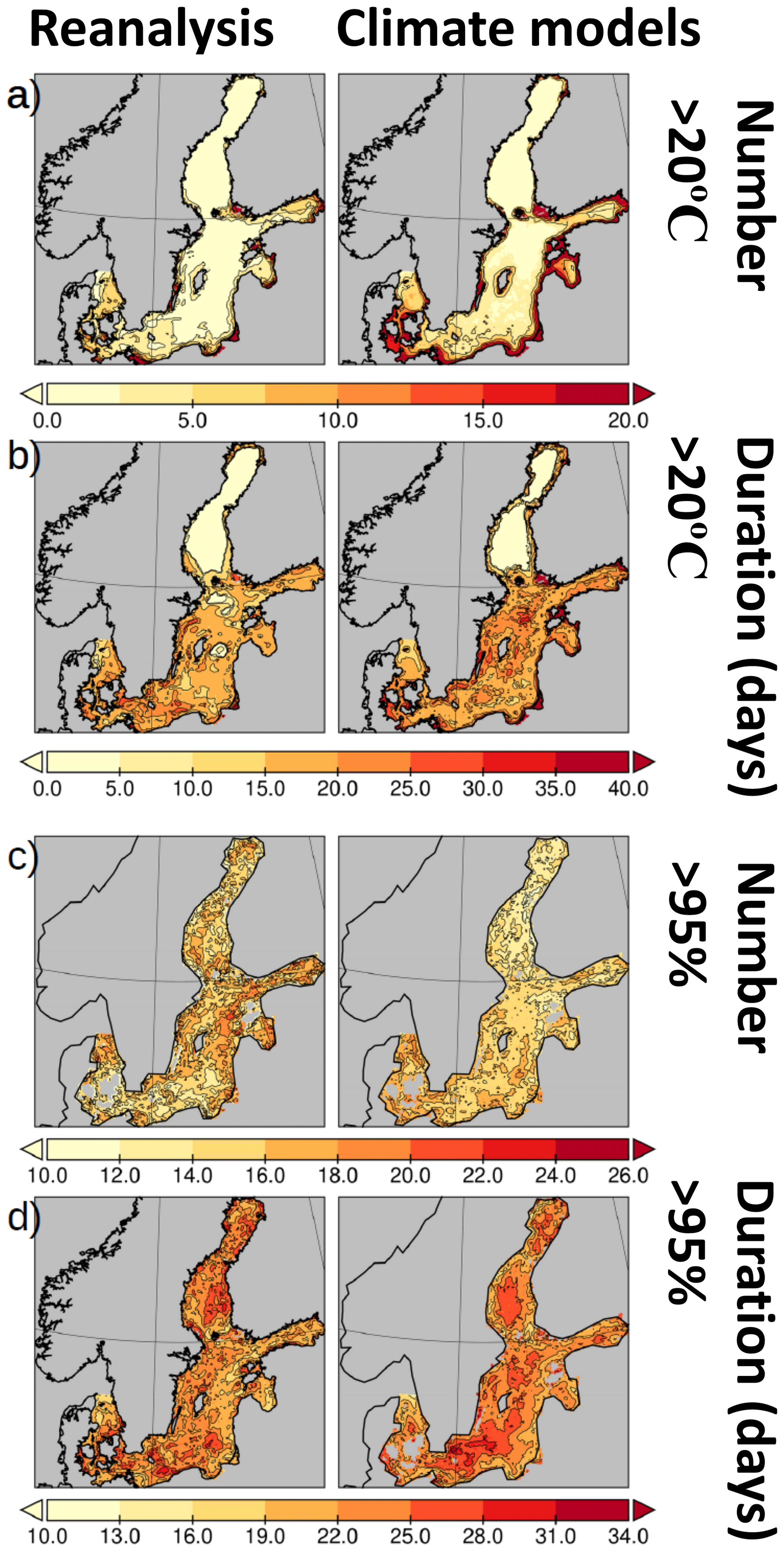
Figure 6(a) Number of >10 d periods in which the SST exceeds 20 ∘C. (b) Average duration of the periods displayed in panel (a). (c) Number of 10 d periods in which the SST exceeds the 95th percentile. (d) Average duration of the periods displayed in panel (c). Left column: reanalysis data (Liu et al., 2017). Right column: ensemble mean of the scenario simulations driven by four ESMs (Saraiva et al., 2019a). The analysis period is 1976–1999. Note the different colour scales used in panels (c) and (d).
The first MHW index uses a fixed threshold that emphasises the environmental impact of the heat waves. In particular, diazotrophic nitrogen fixation becomes effective at higher temperatures. The spatial pattern of MHWs is strongly related to the simulated SST. Figure 6a shows that MHWs are mostly absent in the open sea of the Baltic Proper and further north in the Gulf of Bothnia, but they are highly abundant in shallow marginal bays such as the Gulf of Finland and Gulf of Riga as well as along the coasts. The MHWs produced by the RCO ensemble mean are generally more frequent and of longer duration than those of the reanalysis data set. Furthermore, the coastal signature of high abundance extends further offshore (Fig. 6a). For the Belt Sea and Bay of Lübeck, this leads to considerable deviations from the reanalysis data set.
The second index is based on a reference climatology, here defined as that of 1976–1999. The number of MHWs (Fig. 6c) correlates negatively with their average duration (Fig. 6d). This is somewhat more pronounced in the reanalysis data set. In general, the patterns obtained with the reanalysis data and the RCO are similar but the amplitude of spatial variance is higher in the former (Fig. 6c), perhaps as it includes small-scale regional observations. In the RCO (Fig. 6d), MHWs in the open sea are of the longest duration, with their interruption likely due to the vertical mixing induced by wind events.
Since MHWs in the Baltic Sea are predominantly a summer phenomenon, the stability of the seasonal thermocline is likely a key element in their dynamics such that processes related to vertical mixing can be considered a benchmark in their simulation by the models. Given that mixing is highly parameterised in current ocean models, the RCO reproduces the spatial patterns of the number and average duration of MHW reasonably well.
In the literature, MHWs in the ECOSUPPORT scenario simulations have not been analysed.
3.1.4 Salinity
The annual mean sea surface salinity (SSS) distribution shows a large north–south gradient mirroring both the input of freshwater from rivers, mostly located in the northern catchment area, and saltwater inflows from the North Sea (Fig. 7). The SSS drops from about 20 g kg−1 in the Kattegat to <2 g kg−1 in the northern Bothnian Bay and eastern Gulf of Finland. For the period 1970–1999, the annual mean SSS of the Baltic Sea including the Kattegat was ∼7.3 g kg−1. Large inflows of heavy saltwater from the Kattegat occasionally ventilate the bottom water of the Baltic Sea, filling its deeper regions (Fig. 7). As tides are almost absent, mixing is limited such that the water column is characterised by a pronounced vertical gradient in salinity, and consequently also in density, between the sea surface and the bottom.

Figure 7Upper panels: annual mean sea surface salinity (SSS) and bottom salinity (BS) (in g kg−1) and the winter (December–February) mean sea level (SL; in cm) in the reanalysis data of 1971–1999 (Liu et al., 2017; from left to right). Note that the model results for sea level are given in the Nordic height system 1960 (NH60) by Ekman and Mäkinen (1996). Lower panels: difference between the climatologies of the ensemble mean of the regionalised ESMs used in BalticAPP (Saraiva et al., 2019a) during the historical period (1976–2005) and those of the reanalysis data.
Probably due to differences in the data of the hydrological model (E-HYPE) compared to observations, SSS in the coastal zone and the Kattegat is on average lower in the CLIMSEA climate models than in the reanalysis data of Liu et al. (2017) (Fig. 7). The spatially averaged, annual mean bias is −0.4 g kg−1. Bottom salinities in the Belt Sea, Great Belt area and the Gotland Basin (especially in the northwestern part) are considerably higher and in the Bornholm Basin considerably lower in the climate models than in the reanalysis data (Fig. 7). The spatially averaged, annual mean bias is +0.3 g kg−1. Hence, vertical stratification in the Belt Sea, Great Belt area and the Gotland Basin is also larger in the climate models than in the reanalysis data, because the difference between surface and bottom salinities is a good proxy for vertical stratification.
In the ECOSUPPORT scenario simulations, SSS is overestimated in the entire Baltic Sea, in particular in its northern and eastern regions (Meier et al., 2011c, 2012c). In both, the ensemble mean bottom salinity and vertical stratification are also overestimated, while the bottom salinity in the eastern Gotland Basin is well reproduced (Meier et al., 2012c).
3.1.5 Sea level
Due to the seasonal cycle in wind speed, with wind directions predominantly from the southwest, the sea level in the Baltic Sea varies considerably throughout the year, with the highest levels (∼40 cm), measured relative to the Kattegat, occurring during winter at the northern coasts of the Bothnian Bay and at the eastern coasts of the Gulf of Finland (Fig. 7). For the period 1976–1999, the annual mean sea level in the Nordic height system 1960 (NH60) as determined by Ekman and Mäkinen (1996) was ∼16 cm, with a horizontal north–south difference of ∼35 cm (not shown). This sea level slope was explained by the lighter brackish water in the northeastern Baltic Sea than in the Kattegat and by wind coming from the southwesterly direction, which pushes the water to the north and east (Meier et al., 2004a).
The differences in the mean sea level between the CLIMSEA climate models and the reanalysis data are small (Fig. 7), and the spatially averaged winter mean bias is only +0.6 cm. Sea levels in some parts of the coastal zone such as the western Bothnian Sea are higher in the climate models than in the reanalysis data, probably due to lower salinities. The negative sea level bias in the eastern Gotland Basin suggests an intensified, basin-wide cyclonic gyre. The seasonal cycle of the ensemble mean sea level is relatively well simulated, but with an overestimated sea level in early spring and an underestimated sea level in summer at all investigated tide gauge locations compared to observations and to a hindcast simulation driven by regionalised ERA-40 data (Fig. 8).
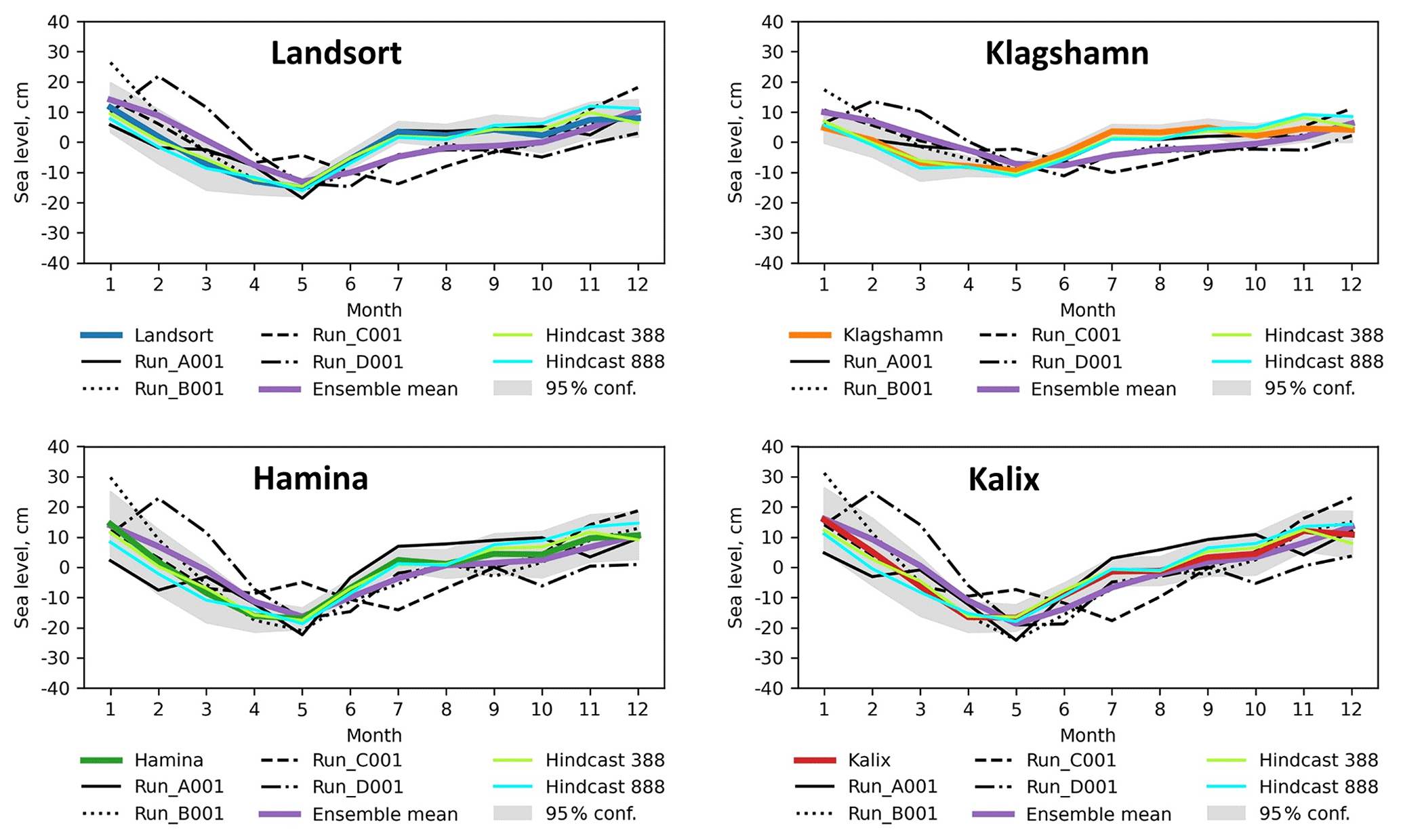
Figure 8Monthly mean sea level according to a hindcast (driven by a regionalised reanalysis of atmospheric surface fields, i.e. RCA4 driven by ERA-40; hindcast 388), reanalysis with the data assimilation of Liu et al. (2017) (hindcast 888) and four climate simulations following Saraiva et al. (2019a) (Run_A001, …, Run_D001), the ensemble mean and observations for the historical period 1976–2005 at the sea level stations Klagshamn, Landsort, Hamina and Kalix (for the locations, see Fig. 1). The 95 % confidence interval of the observations is shown as a grey-shaded area.
In the ECOSUPPORT scenario simulations, sea levels were not systematically analysed. In one of the three models (RCO-SCOBI), seasonal mean biases were comparable to the biases in the CLIMSEA scenario simulations (Meier et al., 2011a).
3.1.6 Oxygen concentration and hypoxic area
Since the 1950s, nutrient inputs into the Baltic Sea have increased due to population growth and intensified fertiliser use in agriculture (Gustafsson et al., 2012; Fig. 3). Nutrient inputs reached their peak in the 1980s but have steadily declined following the implementation of nutrient input abatement strategies. Nonetheless, since the 1960s, the bottom water of the Baltic Sea below the permanent halocline has been characterised by oxygen depletion and large-scale hypoxia (Fig. 9).
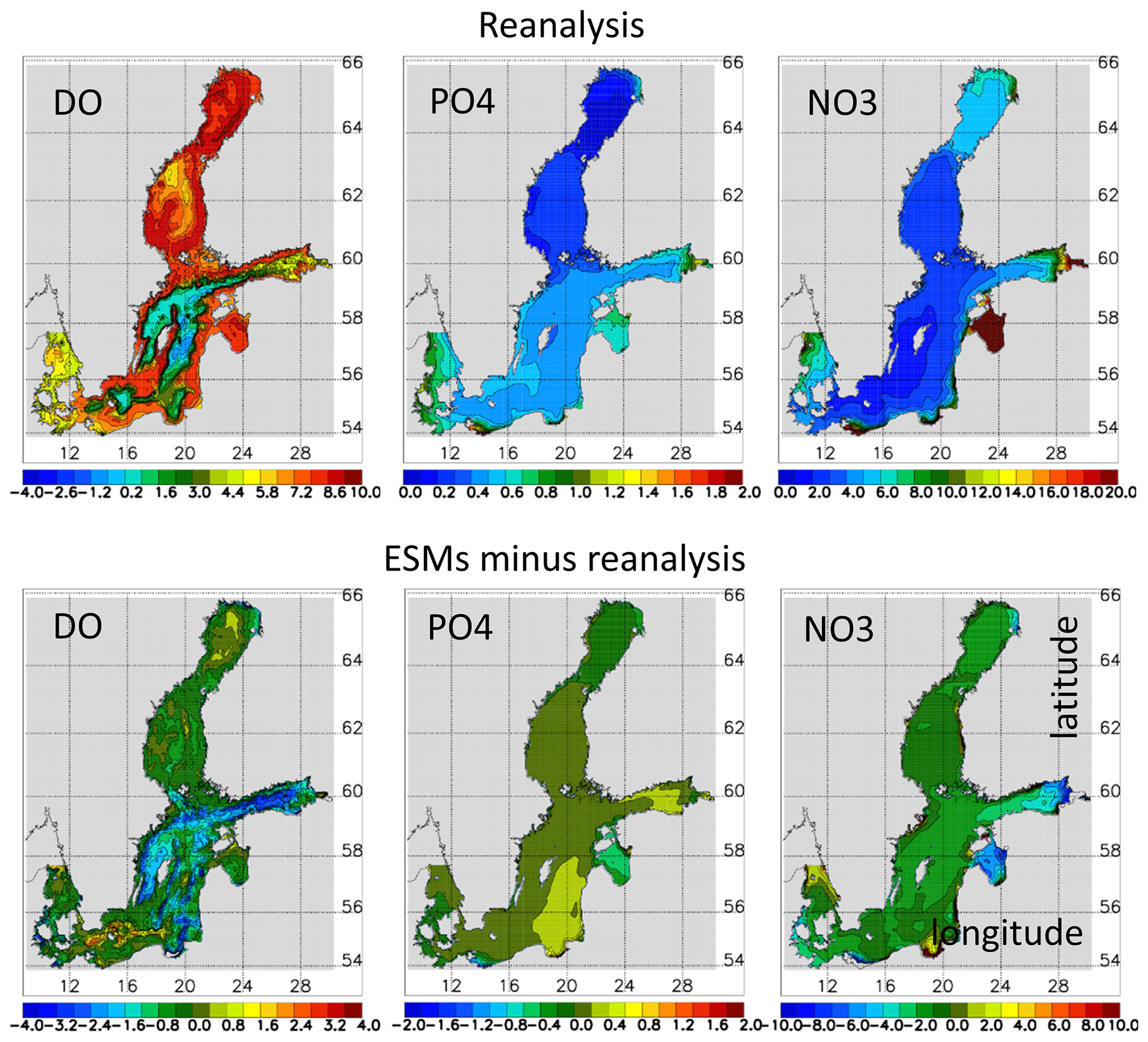
Figure 9Upper panels: summer (June–August) mean bottom dissolved oxygen (DO) concentrations (in mL L−1), winter (December–February) mean surface phosphate (PO4) concentrations (in mmol P m−3) and winter (December–February) mean surface nitrate (NO3) concentrations (in mmol N m−3) in the reanalysis data of 1976–1999 (Liu et al., 2017). Negative oxygen concentration equivalents denote hydrogen sulfide concentrations, with 1 mL H2S L−1 = −2 mL O2 L−1. Nutrient concentrations are vertically averaged for the upper 10 m. Lower panels: difference between the climatologies of the ensemble mean of the ESMs (Saraiva et al., 2019a) and those of the reanalysis data of the historical period (1976–2005).
Consistent with the stratification biases in the deeper sub-basins of the Baltic Sea, summer bottom oxygen concentrations in the Bornholm Basin are higher and those in the Gotland Basin lower in the CLIMSEA/BalticAPP climate simulations than in the reanalysis data of Liu et al. (2017) (Fig. 9). The stronger vertical stratification, especially at the halocline depth, hampers vertical fluxes of oxygen, causing prolonged residence times and lower bottom oxygen concentrations. Spatially averaged biases during winter, spring, summer and autumn and in the annual mean are small but systematic: −0.6, −0.7, −0.7, −0.5 and −0.6 mL L−1, respectively.
In the ECOSUPPORT scenarios, the ensemble mean deep-water oxygen concentration in the eastern Gotland Basin is slightly higher (but within the range of natural variability) and that in the Gulf of Finland significantly lower than determined from observations (Meier et al., 2011b, 2012d).
3.1.7 Nutrient concentrations
Nutrient (i.e. phosphorus and nitrogen) content in the surface layer during winter is a good indicator of the intensity of the following spring bloom. Sea surface mean winter concentrations of phosphate and nitrate are highest in the coastal zone, in particular close to the mouths of the large rivers in the southern Baltic Sea that transport elevated inputs of nutrients into the sea (Fig. 9).
For the historical period of 1976–1999, winter surface phosphate concentrations according to the climate simulations are relatively close to those of the reanalysis data (Fig. 9). The concentrations differ substantially only in those coastal regions influenced by large rivers, such as those affected by discharges of the Oder, Vistula and Pärnu rivers. Spatially averaged biases are largest during summer and autumn, with an average bias in summer of +0.2 mmol P m−3.
Likewise, winter surface nitrate concentrations in the simulations are close to those in the reanalysis data but in coastal regions they differ due to differences in the inputs from large rivers (Fig. 9). This is exemplified by the Gulf of Riga and the eastern Gulf of Finland, where the large differences between them are due to inputs from the Neva River. Spatially averaged biases during winter, spring, summer, autumn and in the annual mean are rather small but systematic: −1.1, −1.3, −0.5, −0.7 and −0.9 mmol N m−3, respectively.
In the ECOSUPPORT scenario simulations, the simulated profiles of phosphate, nitrate and ammonium are within the range of observations for 1978–2007, except in the case of phosphate in the Gulf of Finland (Meier et al., 2012d). According to hindcast simulations, the biases in the coupled physical–biogeochemical models of the Baltic Sea relative to the standard deviations of observations are larger for the northern Baltic Sea than for the Baltic Proper (Eilola et al., 2011).
3.1.8 Phytoplankton concentrations
During the period 1976–1999, dense phytoplankton blooms were confined to the coastal zone, i.e. the area with the highest nutrient concentrations (Fig. 10). Water transparency, measured by Secchi depth, is lower in the Baltic Sea than in the open ocean (Fleming-Lehtinen and Laamanen, 2012), and for the period 1970–1999 the annual mean Secchi depth averaged for the entire Baltic Sea, including the Kattegat, was only ∼6.6 m. The Secchi depth is also much smaller in the coastal zone than in the open Baltic Sea (Fig. 10), and in the northern Baltic Sea than in the Gotland Basin, attributable to yellow substances originating from land (Fleming-Lehtinen and Laamanen, 2012).
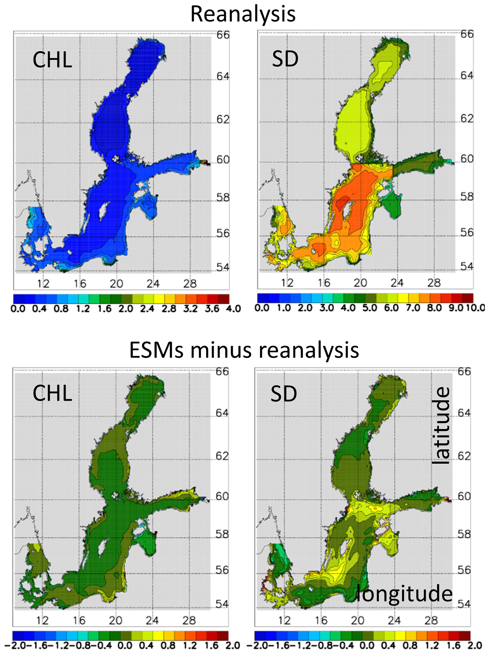
Figure 10Upper panels: annual mean phytoplankton concentrations (CHL; in mg Chl m−3) and annual mean Secchi depth (SD; in m) of the reanalysis data for 1976–1999 (Liu et al., 2017). Phytoplankton concentrations are vertically averaged for the upper 10 m. Since in the calculation of the Secchi depth as background only one value for the concentration of yellow substances per sub-basin is available, artificial borders between sub-basins become visible. Lower panels: difference between the climatologies of the ensemble mean of the ESMs (Saraiva et al., 2019a) and those of the reanalysis data for the historical period (1976–2005).
Due to nutrient concentration biases, the annual mean surface phytoplankton concentrations of the simulations are close to those of the reanalysis data of Liu et al. (2017) but they deviate in coastal regions (Fig. 10). Spatially averaged biases during winter, spring, summer and autumn and in the annual mean are relatively small: +0.02, −0.1, −0.009, +0.06 and −0.008 mg chlorophyll (Chl) m−3, respectively. Note that the reanalysis data of Liu et al. (2017) assimilate nutrient and oxygen concentrations but not chlorophyll data.
Similar results are found for the mean biases in the simulated Secchi depths (Fig. 10). In climate simulations, Secchi depths are systematically deeper in the regions south of Gotland and at the entrance to the Gulf of Finland (northeastern Gotland Basin) than elsewhere in the Baltic Sea. Spatially averaged biases during winter, spring, summer and autumn and in the annual mean are +0.2, +0.4, +0.06, +0.1 and +0.2 m, respectively.
Compared to the Secchi depth data from HELCOM (HELCOM, 2013a; their Table 4.3) and Savchuk et al. (2006; their Table 3), the CLIMSEA climate simulations under- and overestimate the Secchi depth in the southwestern and northern Baltic Sea, respectively, while in the Gotland Basin the model results well fit the observations (Meier et al., 2019a).
In the ECOSUPPORT scenario simulations, Secchi depth was not compared with observations.
3.1.9 Biogeochemical fluxes
An evaluation of biogeochemical fluxes, such as primary production and nitrogen fixation, is difficult because observations are lacking. An exception is the study by Hieronymus et al. (2021), in which historical simulations with RCO-SCOBI were compared with in situ observations of nitrogen fixation. The RCO-SCOBI model includes a cyanobacteria life cycle (CLC) model (Hense and Beckmann, 2006, 2010) driven by reconstructed atmospheric and hydrological data. The authors found a satisfactory agreement, with the results mainly within the uncertainty range of the observations. However, simulated monthly mean nitrogen fixation during 1999–2008 showed a prolonged peak period in July and August, whereas according to observations the peak was mostly confined to July. It should be noted that the RCO-SCOBI version used in the scenario simulations discussed here (e.g. Saraiva et al., 2019a) does not contain a CLC model.
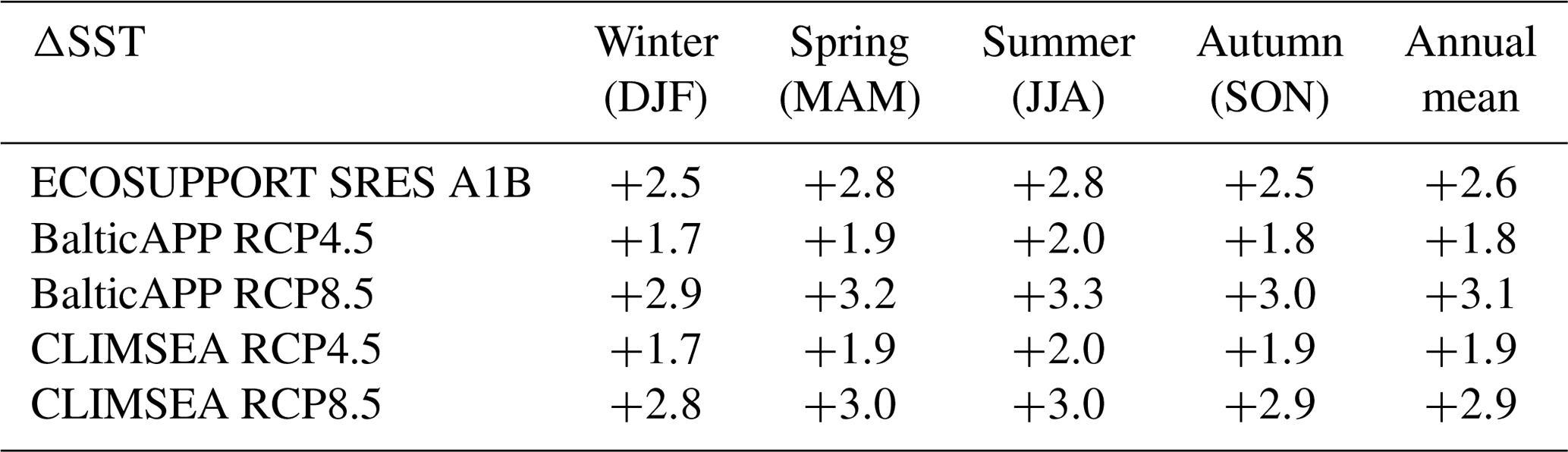
Table 7Ensemble mean changes in sea surface temperature (SST; in ∘C) in the ECOSUPPORT, BalticAPP RCP4.5, BalticAPP RCP8.5, CLIMSEA RCP4.5 and CLIMSEA RCP8.5 scenario simulations averaged for the Baltic Sea including the Kattegat (data sources: Meier et al., 2011b, 2021; Saraiva et al., 2019a). The changes are calculated between historical (1978–2007 in ECOSUPPORT and 1976–2005 in BalticAPP/CLIMSEA) and future (2069–2098) periods. (DJF is December, January, February; MAM is March, April, May; JJA is June, July, August; SON is September, October, November.)
3.2 Future period
3.2.1 Water temperature
Annual and seasonal mean changes
In Figs. 11–12 and Table 7, annual and seasonal mean SST changes between 1976–2005 and 2069–2098 in RCO-SCOBI are depicted and quantified respectively. The maximum seasonal warming signal propagates between winter and summer from the Gulf of Finland via the Bothnian Sea into the Bothnian Bay (Fig. 11). Maximum warming occurs during summer in the Bothnian Sea and Bothnian Bay. The seasonal patterns of RCP4.5 and RCP8.5 are similar although warming is greater in the latter. As SLR has almost no impact on SST changes, BalticAPP and CLIMSEA scenario simulations yield similar results (not shown). The warming level according to ECOSUPPORT is between that predicted by CLIMSEA/BalticAPP RCP4.5 and RCP8.5 because the GHG emissions of the A1B scenario, which forces the ECOSUPPORT ensemble2, are between those of the RCP4.5 and RCP8.5 scenarios.
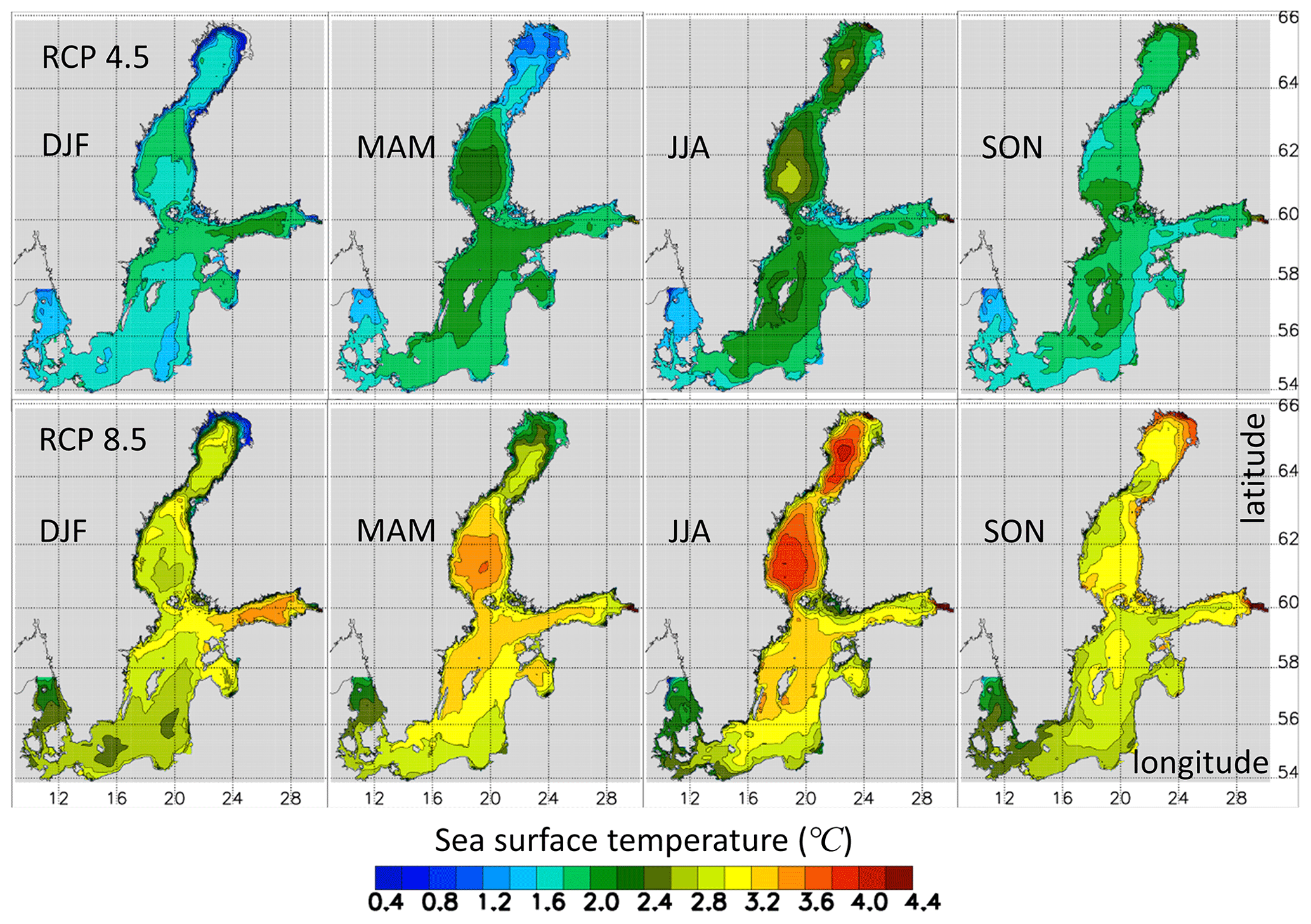
Figure 11Changes in seasonal mean SST as simulated by the CLIMSEA ensemble. From left to right, mean SST changes (in ∘C) in winter (December, January and February; DJF), spring (March, April and May; MAM), summer (June, July and August; JJA) and autumn (September, October and November; SON) between 1976–2005 and 2069–2098 under RCP4.5 (upper panels) and RCP8.5 (lower panels). (Source: Meier et al., 2021; their Supplementary Fig. 1 distributed under the terms of the Creative Commons CC-BY 4.0 License, http://creativecommons.org/licenses/by/4.0/, last access: 6 January 2022.)
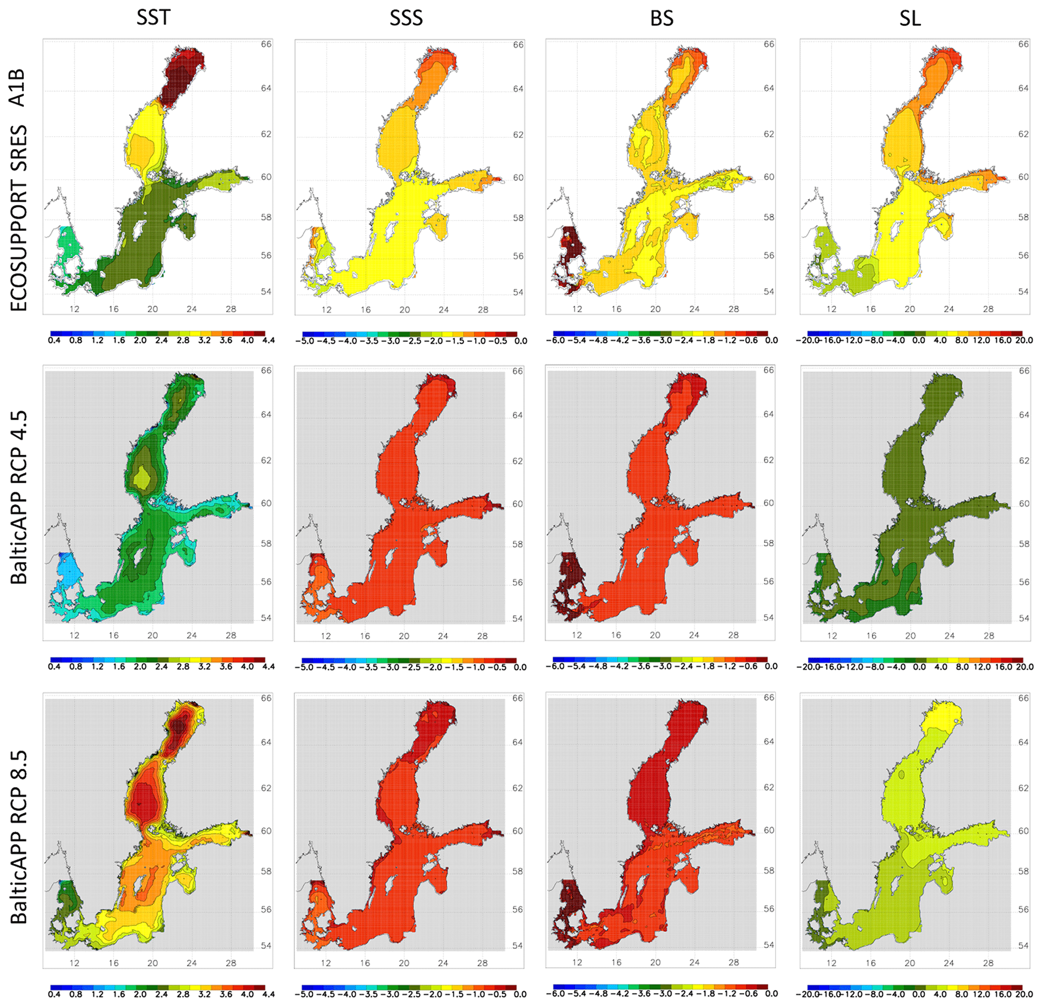
Figure 12From left to right, changes in the mean SST (∘C) in summer (June–August), the annual mean sea surface salinity (SSS; g kg−1), annual mean bottom salinity (BS; g kg−1) and winter (December–February) mean sea level (SL; cm) between 1978–2007 and 2069–2098. From top to bottom, the results of the ensembles ECOSUPPORT (white background, Meier et al., 2011b), BalticAPP RCP4.5 (grey background, Saraiva et al., 2019a) and BalticAPP RCP8.5 (grey background, Saraiva et al., 2019a).
In the CLIMSEA/BalticAPP RCSM projections, the annual mean SST changes in the Baltic Sea driven by four ESMs, i.e. MPI-ESM-LR, EC-EARTH, IPSL-CM5A-MR, HadGEM2-ES, under the RCP8.5 scenario are +2.3, +3.7, +3.5 and +4.7 ∘C respectively (Gröger et al., 2019). Thus, the ensemble mean change is +3.5 ∘C. The corresponding ensemble mean change in the RCO-SCOBI scenario simulations is smaller, +2.9∘. Different MLDs, vertical stratification and sea-ice cover in the two ocean models, RCO-SCOBI and NEMO, may explain the different responses. Indeed, a comparison of the MLD between the two models reveals a shallower MLD in the RCSM than in RCO-SCOBI (not shown), which argues for a higher sensitivity of the RCSM to climate warming.
While the spatial patterns of the SST changes in the scenario simulations of ECOSUPPORT (e.g. Meier et al., 2012c) and CLIMSEA (e.g. Saraiva et al., 2019b) are similar, the uncertainties due to the applied global (Meier et al., 2011a) or regional (Meier et al., 2012b) model are in some cases considerable. Of note is the summer ensemble range of the various GCMs (Meier et al., 2011a). The strong dependence on forcing is seen by comparing the different warming levels in the RCP4.5 and RCP8.5 scenarios shown in Fig. 12.
Trends
Since SLR and nutrient input scenarios have a negligible impact on SST changes, only the RCP4.5 and RCP8.5 scenarios in CLIMSEA/BalticAPP are compared. The multi-model mean of the annual mean SST trends averaged over the Baltic Sea is ∼0.18 and ∼0.35 ∘C per decade in the RCP4.5 and RCP8.5 scenarios respectively (Fig. 13f and k). At the Baltic Sea scale, seasonal SST trends based on annual values vary only slightly (±0.01 ∘ C per decade in both scenarios). However, at the sub-basin scale, seasonal variations are much stronger, reaching ±0.05 ∘C per decade in the northern Baltic Sea, with a maximum in summer (Fig. 13). This summer maximum can be explained by the projected decline in sea-ice cover in summer, as occurred during the period 1850–2008 (Kniebusch et al., 2019).
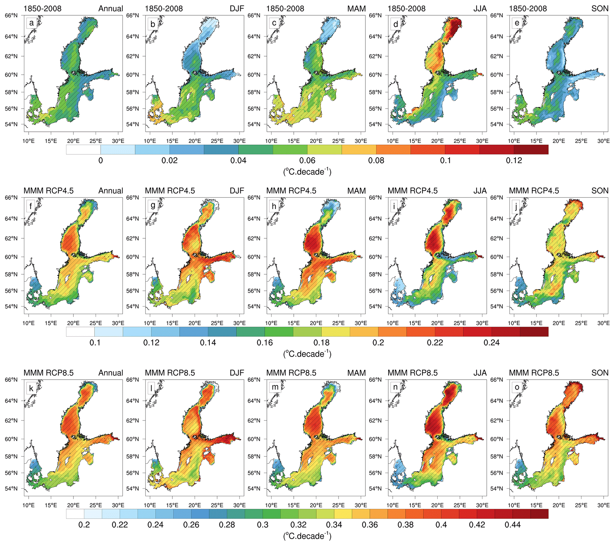
Figure 13Multi-model mean (MMM) of annual (a, f, k) and seasonal (b–e, g–j, l–o) SST trends (in ∘C per decade) computed for the period 1850–2008 (a–e), 2006–2099 in the RCP4.5 (f–j) and RCP8.5 (k–o) scenarios. Hatched areas represent the regions where the trend is statistically significant (p<0.05, Mann–Kendall test). Data for historical reconstructions and projections are from Meier et al. (2019d) and Saraiva et al. (2019a), respectively (cf. Dutheil et al., 2021).
As seen in Fig. 14, the relative SST trends indicate faster warming of the northern than the southern Baltic Sea (0.02 and 0.04 ∘C per decade in the RCP4.5 and RCP8.5 scenarios respectively), with the largest trends, calculated over the entire period 2006–2099, reaching ∼0.24 and ∼0.45 ∘C per decade in RCP4.5 and RCP8.5, respectively. However, a calculation of the SST trends by 30-year slice periods every 10 years over the entire period shows that annual SST trends are variable over time (not shown). The natural variability appears to modulate these trends, with successive periods of increasing and decreasing SST trends over a period of about 30 years. For example, in the RCP8.5 scenario, SST trends gradually increase over the first 50 years of the period, reaching a maximum of 0.5 ∘C per decade between 2046 and 2075, before declining slightly from 2060 onwards. As in the RCP4.5 scenario, this is a result of the pronounced natural variability in this scenario. Despite the robustness of the spatial pattern of the SST trends (p<0.05 everywhere), an analysis of SST trends for the four ESM forcings reveals an important dependency of those trends on atmospheric forcings, with a spread of ±0.06 ∘C per decade from the multi-model mean of both scenarios (not shown).
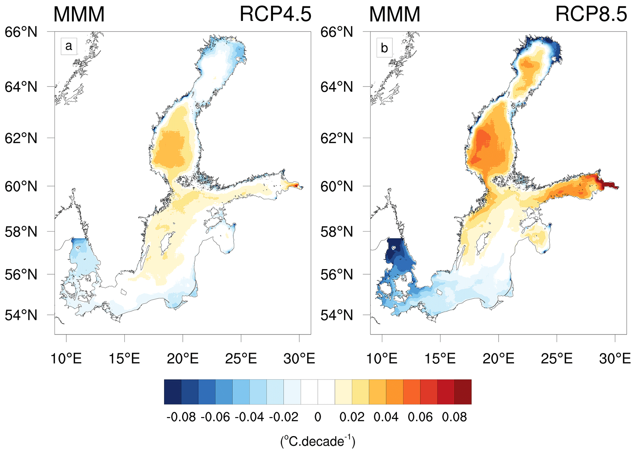
Figure 14MMM of the annual SST trends relative to the spatial average (in ∘C per decade) for the (a) RCP4.5 and (b) RCP8.5 scenario simulations. (Data source: Saraiva et al., 2019a.)
At an annual timescale, the variability in the air temperature, through the sensible heat fluxes, is the main driver of the Baltic Sea's SST (Kniebusch et al., 2019), illustrated here by the high variance of SST explained by air temperature (between 0.85 and 0.95, Fig. 15). The minimum of variance explained is located in the Bothnian Bay, where the sea-ice cover isolates seawater from the air in winter.
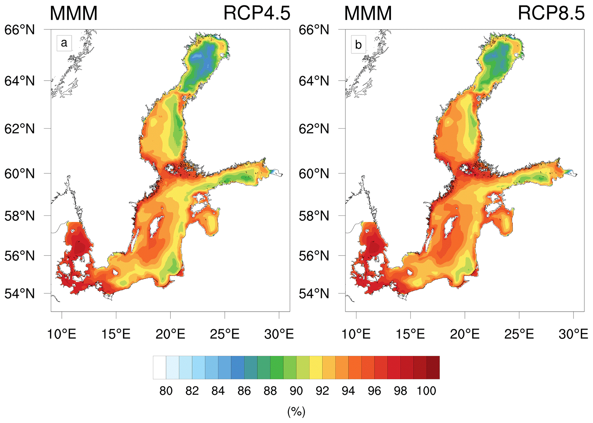
Figure 15MMM explained variance (in percent) between the monthly mean SST and the forcing air temperature over the period 2006–2099 in the (a) RCP4.5 and (b) RCP8.5 scenario simulations. (Data source: Saraiva et al., 2019a.)
The processes responsible for the SST trends were analysed using a rank analysis of atmospheric variables (i.e. latent heat fluxes, cloud cover and u−v wind components) following Kniebusch et al. (2019; Fig. 16). The second parameter (after SAT) explaining the variability in the SST differs according to the location and ESM. Nevertheless, in all ESMs and in both RCP scenarios, zonal and meridional wind components are the variables that best correlate with SST along most of the coastal areas, probably because of upwelling. In the open sea of the Baltic Proper and in the Bothnian Bay, the second most important variable is cloudiness. This is also the case in the Bothnian Sea under the RCP4.5 scenario. However, in RCP8.5, the second most important variable at this location is the latent heat flux. The difference is perhaps due to the absence of sea ice and therefore the amplified air–sea exchange, under RCP8.5.

Figure 16Results of the cross-correlation analysis of the detrended SST (monthly mean) with the wind components, latent heat flux and cloudiness. Maps of the atmospheric drivers with the highest cross-correlations in the RCP4.5 (a–d) and RCP8.5 (e–h) scenarios for various GCM forcings (Saraiva et al., 2019a). From left to right: MPI-ESM-LR, EC-EARTH, IPSL-CM5A-MR, HadGEM2-ES.
In the vertical, temperature trends are larger in the surface layer than in the winter water of the Baltic Sea above the halocline, thus causing a more intense seasonal thermocline (see Sect. 3.2.2). Surface layer trends are largest in spring and summer (not shown). Elevated trends also characterise deep water, due to the influence of saltwater inflows that will be warmer in a future climate because they originate from the shallow entrance area and occur mainly in winter. Hence, in sub-basins that are sporadically ventilated by lateral saltwater inflows, such as the Bornholm Basin and the Gotland Basin, the deep water below the halocline will warm more than the overlaying intermediate layer water.
In the literature, trends in ECOSUPPORT scenario simulations have not been analysed.
3.2.2 Mixed-layer depth
Figure 17 shows the changes in the MLD. During winter, reduced sea-ice cover in the Bothnian Sea and Bothnian Bay favours a widespread deepening of their MLDs, likely caused by wind-induced mixing. In spring, the most pronounced feature is a strong shallowing of the MLD in the Bothnian Sea, probably attributable to the radiative fluxes that warm the surface layer and to less thermal convection (Hordoir and Meier, 2012). During the historical period, water temperatures in this area were between 2.0 and 3.0 ∘C (Fig. 4). Thus, in the future, surface water warming between 1.6 and 2.4 ∘C (Fig. 11) may hamper thermal convective mixing.
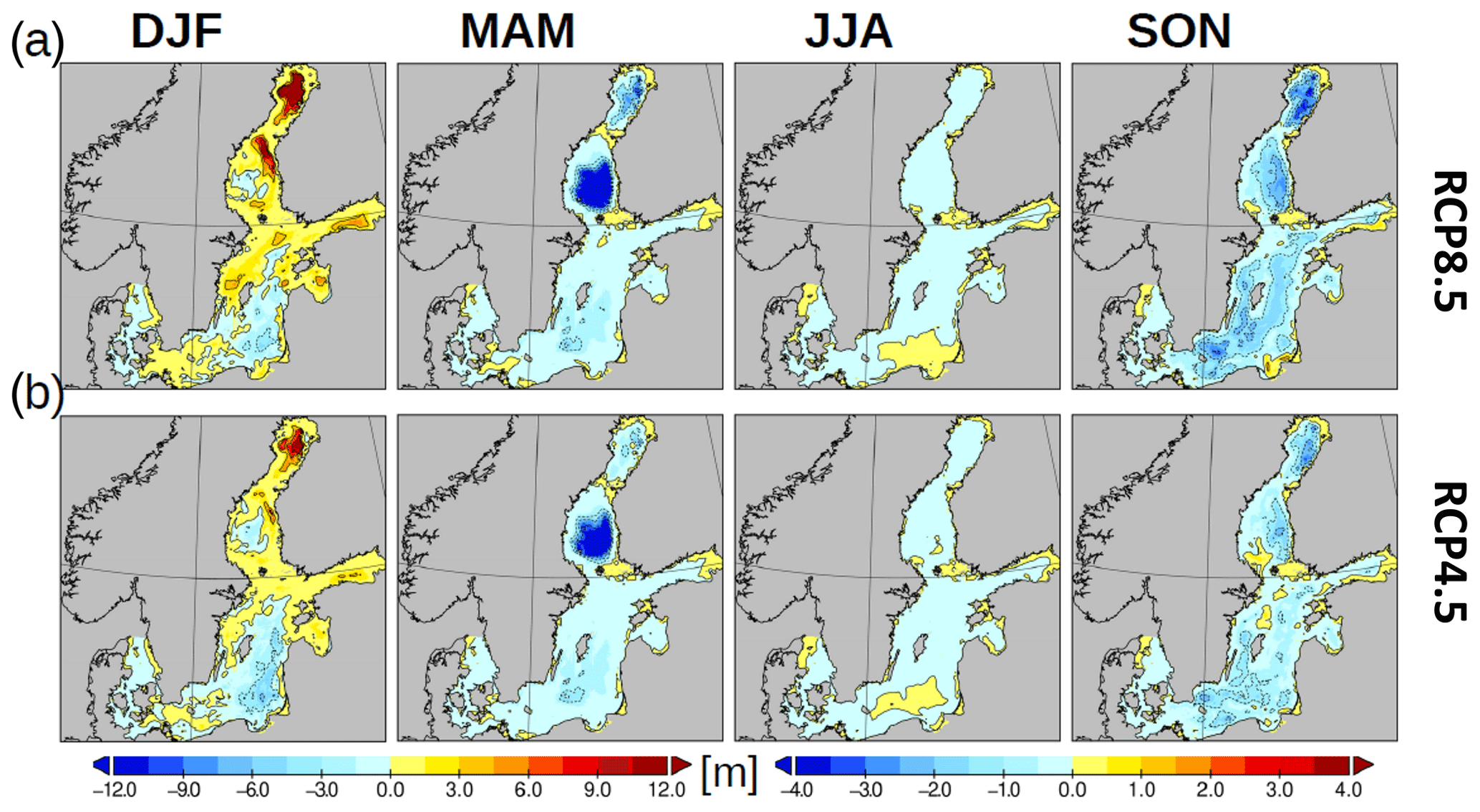
Figure 17Mixed-layer depth calculated according to the criterion of de Boyer Montégut et al. (2004). Shown are the ensemble average changes of four different ESMs between 1976–2005 and 2069–2098 with the mean sea level rises (a) 0.90 m (RCP8.5) and (b) 0.54 m (RCP4.5). (Data source: Meier et al., 2021.)
The changes during summer are less pronounced. In contrast to winter, there is an overall shallowing in the entire Baltic Sea. This is in agreement with a shallower, more intense thermocline in warming scenarios, as suggested by Gröger et al. (2019), and it is a common feature among the projections, because the changes in wind speed are small (Christensen et al., 2021). Autumn is primarily characterised by a prolongation of the thermal stratification, leading to an overall shallower MLD than during the historical period.
While Hordoir et al. (2018, 2019) speculated that these changes in thermocline depth during summer will impact the vertical overturning circulation, the meridional overturning circulation in the Baltic Proper does not show a clear signal but rather a northward expansion of the main overturning cell (Gröger et al., 2019). Indeed, the effect is expected to be small (Placke et al., 2021).
3.2.3 Marine heat waves
The number of MHWs within climatological 30-year time slices is shown in Fig. 18. Under historical climate conditions, MHWs are virtually absent in open ocean areas. They are most frequent in shallow regions and more abundant along the eastern (Baltic states) than the western (Swedish) coasts, which may reflect the greater frequency of coastal upwelling events along the western than the eastern coasts of the Baltic Sea. Even under the RCP4.5 scenario, wide areas of the Baltic Proper are affected by MHWs roughly once a year. The strongest response is projected for the high-emission RCP8.5 scenario and specifically in marginal basins such as the Gulf of Riga and the Gulf of Finland, where in the future MHWs will occur two or three times per year. Not only the frequency but also the average duration of the MHWs will increase with climate warming. Under RCP8.5, MHWs of ∼20 d duration will occur even in the open Gulf of Bothnia (Fig. 18). This increase in MHWs is likewise linked to an increased frequency of tropical nights in the Baltic Sea (Meier et al., 2019a; Gröger et al., 2021b).
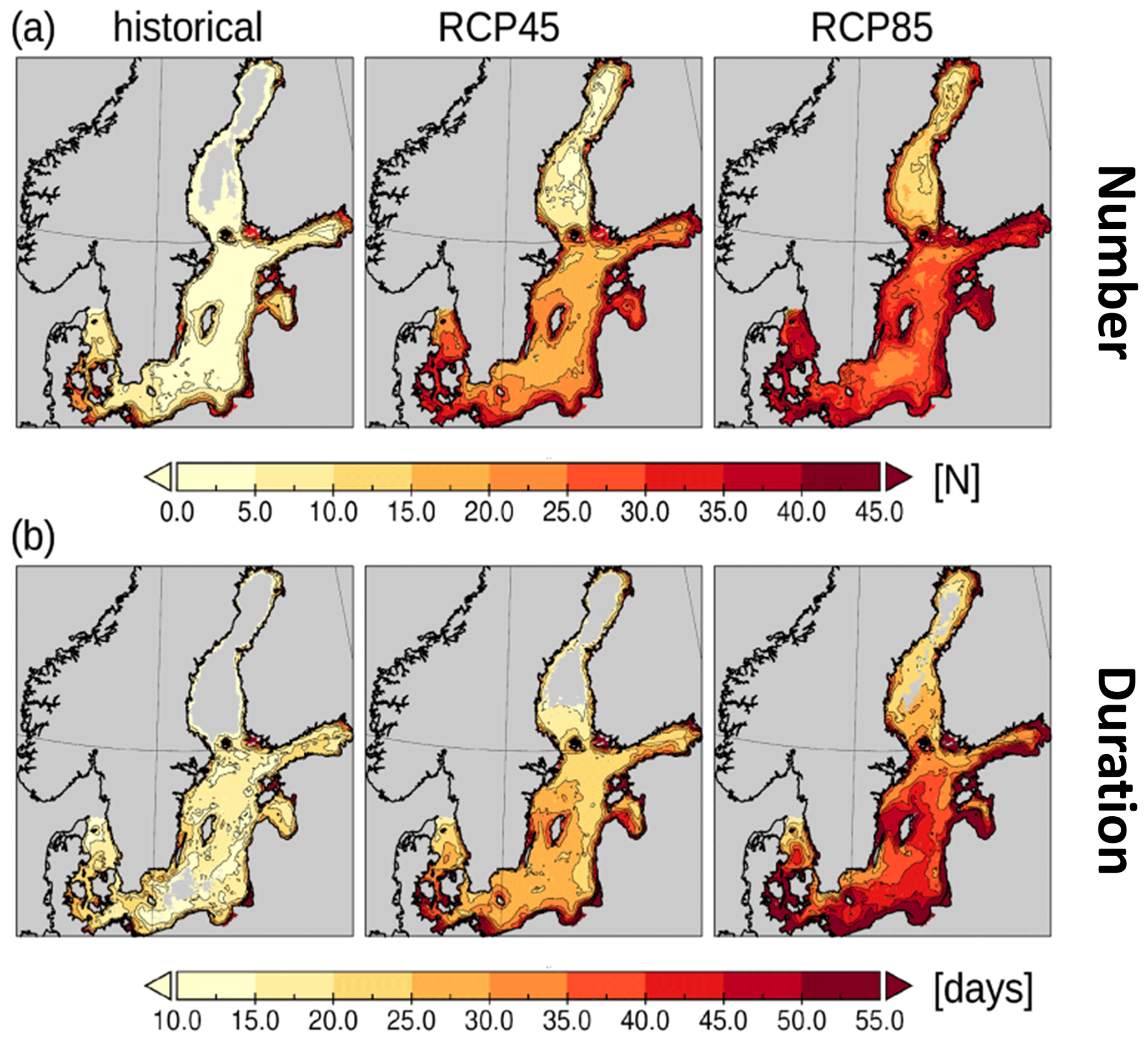
Figure 18(a) Number of heat waves (defined as the number of periods ≥10 d in which the water temperature is ≥20 ∘C) for historical (1976–2005) and future (2069–2098) climates. (b) Average duration of the heat waves. Note that no temperature bias adjustment was done prior to the analysis. Shown are the ensemble averages of four different ESMs with the mean sea level rises (a) 0.54 m (RCP4.5) and (b) 0.90 m (RCP8.5). (Data source: Meier et al., 2021.)
MHWs can also be analysed by calculating them with respect to the 95th percentile temperature of the historical reference climate (Fig. 19). For the historical climate, the average duration of MHWs in most regions is <20–30 d, although in the southern Baltic Sea, especially west of the Baltic Proper, MHWs are more frequent. However, the climate change signal is characterised by MHWs that are both more frequent and of longer duration. In RCP4.5, MHWs in the Baltic Sea occur at least every year. The strongest increase in frequency is near the coasts, but the average duration increases less than in the open sea (Fig. 19). This is probably related to repeated cold-water entrainments from the open sea that interrupt warm periods because of the larger variability in the coastal zone than in the open sea. In addition, with their lower heat storage capacity, shallow areas are more sensitive to cold weather events and the associated oceanic heat loss.
Table 8Ensemble mean changes in annual mean sea surface salinity (SSS; in g kg−1), annual mean bottom salinity (BS; in g kg−1) and winter mean sea level (SL) relative to the global mean SL (in cm) in ECOSUPPORT, BalticAPP RCP4.5, BalticAPP RCP8.5, CLIMSEA RCP4.5 and CLIMSEA RCP8.5 scenario simulations averaged for the Baltic Sea including the Kattegat. For CLIMSEA, both the ensemble mean and the high SL scenarios are listed. In ECOSUPPORT and BalticAPP/CLIMSEA, the changes between 1978–2007 and 2069–2098 and between 1976–2005 and 2069–2098 were calculated, respectively. (Data sources: Meier et al., 2011b, 2021; Saraiva et al., 2019a.)

3.2.4 Salinity
In the CLIMSEA ensemble, salinity changes are not robust; i.e. the ensemble spread is larger than the signal (Meier et al., 2021). Under both RCP4.5 and RCP8.5, the ensemble mean salinity change is small because the impact on salinity of the projected increase in total river runoff from the entire catchment (Fig. 3) is approximately compensated by the impact of larger saltwater inflows due to the projected SLR (Table 8). Hence, compared to previous studies such as those by Meier et al. (2011b; ECOSUPPORT) and Saraiva et al. (2019a; BalticAPP; Fig. 12), the ensemble mean salinity changes in CLIMSEA are much smaller (Table 8). In idealised sensitivity experiments performed with the RCO-SCOBI model for the period 1850–2008 (Meier et al., 2017, 2019d), the change in the average Baltic Sea salinity (1988–2007) increased linearly with SLR and at a rate of ∼1.4 g kg−1 m−1 (Table 9).
Table 9Salinity changes averaged for the Baltic Sea in 1988–2007 relative to 1850 as a function of sea level rise (SLR). In the reference simulation, the mean salinity is 7.42 g kg−1. In method 1, the increase in the water level was added to the first vertical grid box of the RCO-SCOBI model, while in method 2 the increase in the water level was evenly divided between the first and second grid boxes.

3.2.5 Sea level
Following global sea level changes, SLR in the Baltic Sea will accelerate (Hünicke et al., 2015; Church et al., 2013; Bamber et al., 2019; Oppenheimer et al., 2019; Weisse and Hünicke, 2019), albeit at a somewhat slower rate than the global mean because of the remote impact of the melting Antarctic ice sheet (Grinsted, 2015). Changes in SLR in the North Atlantic (and the Baltic Sea) will be larger in response to the melting of the Antarctic ice sheet than to the melting of Greenland, due to gravitational effects. For a mid-range scenario, SLR in the Baltic Sea is projected to be ∼87 % of the global mean (Pellikka et al., 2020). Land uplift will partly, or even more than fully, compensate for the eustatic SLR, in particular in the northern Baltic Sea (e.g. Hill et al., 2010). In RCP2.6 and RCP8.5, the global mean sea level in 2100 is 43 and 84 cm higher than during the period 1986–2005 (Oppenheimer et al., 2019). For these two scenarios, likely ranges are 29–59 and 61–110 cm, respectively. Bamber et al. (2019) assessed ice sheet dynamics in detail and subsequently estimated global-median SLRs in 2100 of 69 and 111 cm for low- and high-case scenarios, respectively. Likely ranges according to the authors were 49–98 and 79–174 cm and very likely ranges 36–126 and 62–238 cm.
In BalticAPP and CLIMSEA scenario simulations, sea level changes are small (Fig. 12, Table 8), whereas in ECOSUPPORT scenario simulations they are larger, particularly in spring, because one member of the multi-model ensemble considers Archimedes' principle (not shown). Note that the sea level changes shown in Fig. 12 consider only changing river runoff, changing wind and melting sea ice as affecting the sea level according to Archimedes' principle (only in the ECOSUPPORT ensemble); as neither the global mean SLR nor land uplift is included, they have to be added (e.g. Meier, 2006; Meier et al., 2004a).
In CLIMSEA, there are no statistically significant seasonal changes in the SLR (Fig. 20). In both GHG concentration scenarios, the largest changes are only about ±5 cm. According to these results, systematic changes in the regional wind field (Christensen et al., 2021) and non-linear effects are negligible. Instead, in the projections, the mean absolute sea level in the Baltic Sea simply follows the mean sea level in the North Atlantic. However, the spatially inhomogeneous isostatic adjustment will considerably alter patterns of sea level changes relative to the sea floor.
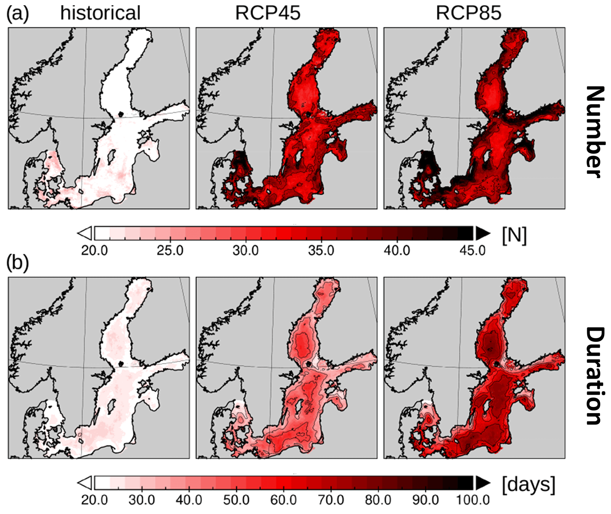
Figure 19Same as in Fig. 18 but for heat waves defined as periods of ≥10 d in which the water temperature exceeded the 95th percentile of the historical reference temperature. (Data source: Meier et al., 2021.)
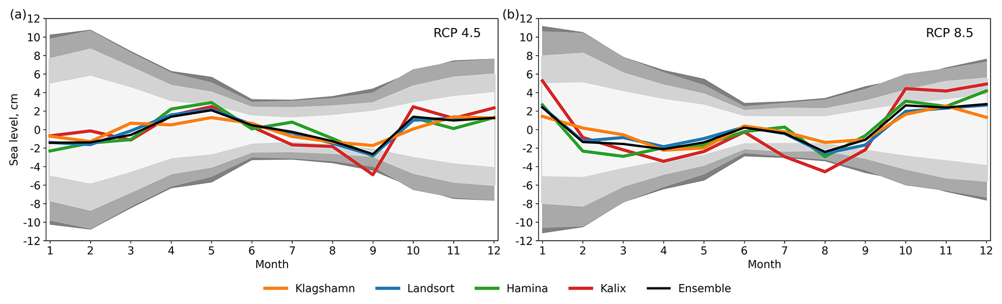
Figure 20Monthly mean sea level changes between 1976–2005 and 2069–2098 at Klagshamn, Landsort, Hamina and Kalix (for the locations, see Fig. 1) for RCP4.5 (a) and RCP8.5 (b). Shown are the changes relative to the mean sea level rise (a) 0.54 m (RCP4.5) and (b) 0.90 m (RCP8.5). Shaded areas in white to dark grey denote 99 % confidence limits of internal variability at Klagshamn to Kalix respectively. The chosen model approach does not indicate any non-linear effects for scenarios with a larger rise in sea level. (Data source: Meier et al., 2021.)
In response to the global mean SLR, the sea level extremes in the Baltic Sea that are rare today will become more common in the future (e.g. Hieronymus and Kalén, 2020). However, changes in sea level extremes relative to the mean sea level will not be statistically significant because wind velocities are projected to remain unchanged (Christensen et al., 2021). The exceptions are areas with sea-ice decline since they are linked to a decrease in atmospheric stability accompanied by increased wind velocities, the result of increases in temperature and turbulent fluxes (Meier et al., 2011c). These increases will mostly translate as changes from calm to light wind conditions as the stable atmospheric boundary layer becomes less stable. For stronger wind conditions related to high sea level extremes, the impact of stratification effects on mixing is small. In addition, open water areas after sea-ice loss have a smaller surface roughness than ice-covered areas, with the reduced surface friction leading to an increase in wind velocities.
Table 10As in Table 8 but showing the ensemble mean changes in the summer mean bottom oxygen concentration (in mL L−1) in ECOSUPPORT, BalticAPP RCP4.5, BalticAPP RCP8.5, CLIMSEA RCP4.5 and CLIMSEA RCP8.5 scenario simulations averaged for the Baltic Sea including the Kattegat. The projected changes depend on the nutrient input scenario: Baltic Sea Action Plan (BSAP), reference (REF), business as usual (BAU) or worst case (WORST). (Data sources: Meier et al., 2011b, 2021; Saraiva et al., 2019a.)
As sea level extremes also depend on the path of low-pressure systems over the Baltic Sea area (Lehmann et al., 2011; Suursaar and Sooäär, 2007), which in a future climate do not show systematic changes (Christensen et al., 2021), changes in sea level extremes relative to the mean sea level are not expected. In addition, a large internal variability at low frequencies prevents the detection of climate-warming-related changes in sea level extremes (Lang and Mikolajewicz, 2019).
3.2.6 Oxygen concentration and hypoxic area
Bottom oxygen concentration
Projected changes in bottom oxygen concentrations differ considerably between ECOSUPPORT and BalticAPP/CLIMSEA scenario simulations, as illustrated for summer (Figs. 21 and 22, Table 10), whereas the differences between BalticAPP (SLR = 0 cm) and CLIMSEA (SLR > 0 cm) scenarios are smaller (Meier et al., 2021). The differences between the ECOSUPPORT and BalticAPP ensembles mainly reflect the different experimental setups of the simulations and the different nutrient input scenarios (Meier et al., 2018a). While in shallow regions without a pronounced halocline future bottom oxygen concentrations decrease in all scenario simulations, due to the lower oxygen saturation concentrations, in deeper offshore regions with a halocline, changes in bottom oxygen concentration depend largely on the nutrient input scenario (Figs. 21 and 22). In ECOSUPPORT scenario simulations, the future bottom oxygen concentration decreases significantly in all scenarios except the BSAP, where in deeper regions it changes only slightly on average (see Meier et al., 2011b). By contrast, in the BalticAPP projections, under the BSAP bottom oxygen concentrations in deeper regions increase considerably, regardless of the degree of warming (see Saraiva et al., 2019a; Meier et al., 2011b). Under RCP4.5, bottom oxygen concentrations increase even under the nutrient inputs of REF and WORST, whereas RCP8.5 predicts slight reductions in the Bothnian Sea and southwestern Baltic Sea, in particular under WORST. Similar results were calculated for the CLIMSEA ensemble (Meier et al., 2021).
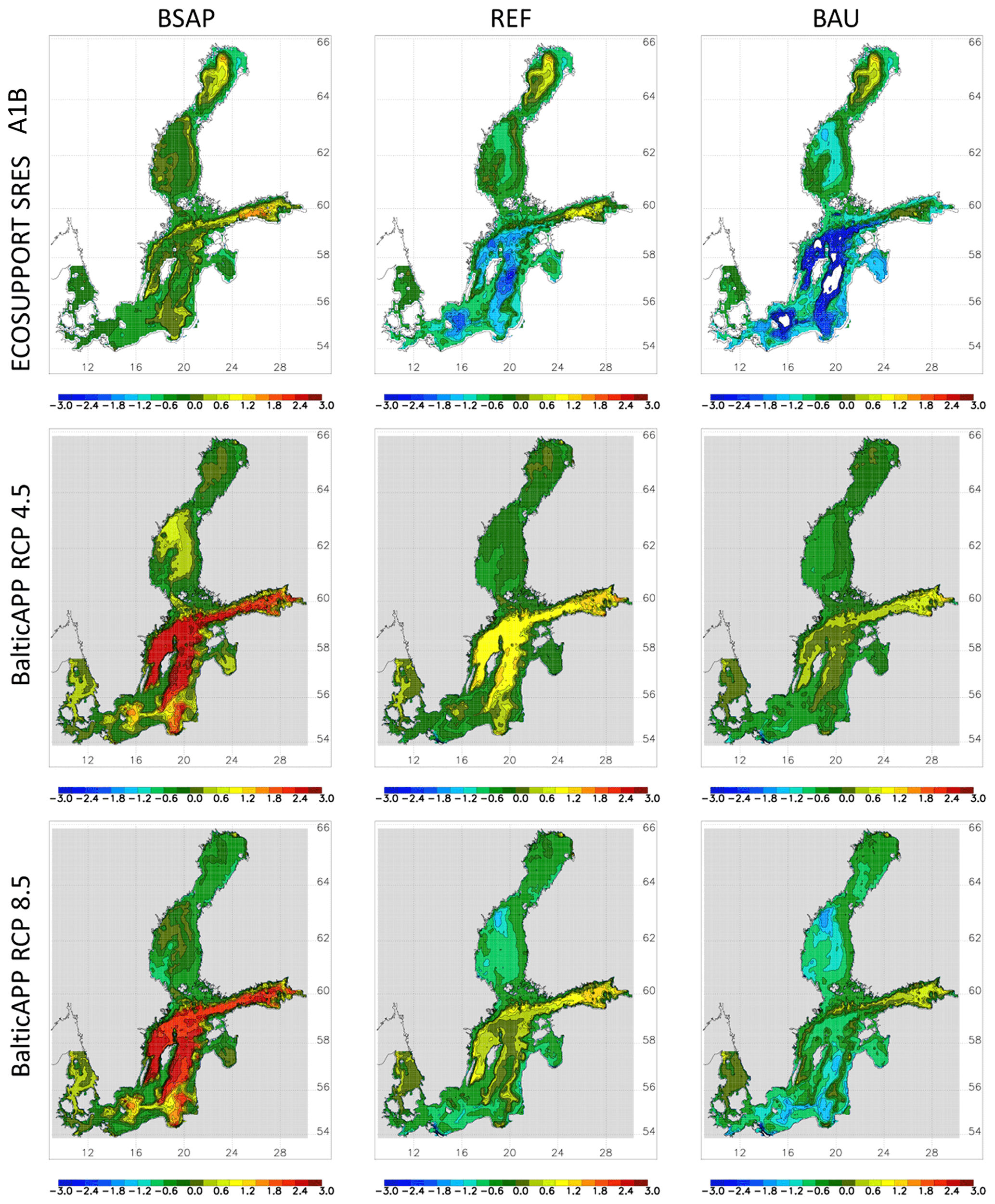
Figure 21Ensemble mean changes in the bottom dissolved oxygen concentration (mL L−1) in summer (June–August) between 1978–2007 and 2069–2098. From left to right, the results of the nutrient input scenarios of BSAP, REF and BAU. From top to bottom, the results of the ensembles ECOSUPPORT (white background; Meier et al., 2011b), BalticAPP RCP4.5 (grey background; Saraiva et al., 2019a) and BalticAPP RCP8.5 (grey background; Saraiva et al., 2019a).
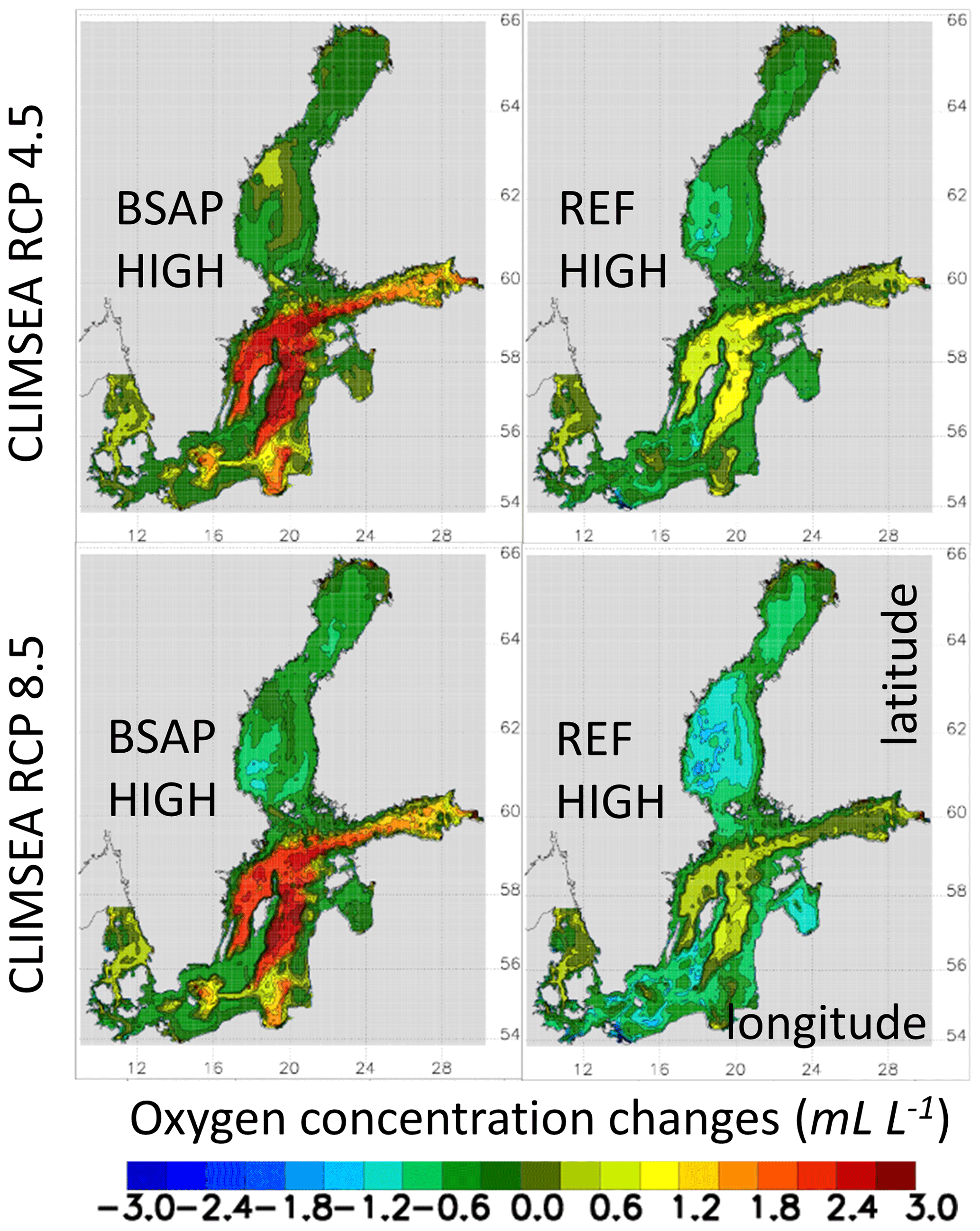
Figure 22As in Fig. 21 but for CLIMSEA RCP4.5 (upper panels) and CLIMSEA RCP8.5 (lower panels) under a high sea level rise scenario, i.e. 1.26 m (RCP4.5) and 2.34 m (RCP8.5). Left and right columns show the BSAP and REF scenarios, respectively. (Source: Meier et al., 2021; their Fig. 5 distributed under the terms of the Creative Commons CC-BY 4.0 License, http://creativecommons.org/licenses/by/4.0/, last access: 6 January 2022.)
Most of the differences in the oxygen concentration changes between the ECOSUPPORT and BalticAPP/CLIMSEA ensembles can be explained as follows. In ECOSUPPORT, changes in nutrient input relative to the historical period 1961–2006, including the observed nutrient inputs averaged from the period 1995–2002, were applied (Gustafsson et al., 2011; Meier et al., 2011b). For the historical period 1980–2002, these inputs were lower than in BalticAPP/CLIMSEA scenario simulations because in the latter the observed monthly nutrient inputs, including the pronounced decline from the peak in the 1980s until the much lower recent values, were used as the forcing (Meier et al., 2018a). Furthermore, in ECOSUPPORT, future nutrient inputs under the BSAP scenario were calculated as relative changes, resulting in higher future inputs than in BalticAPP/CLIMSEA, in which absolute values of the BSAP were applied.
Hence, the reductions between future and historical nutrient inputs are smaller in ECOSUPPORT under the BSAP than in BalticAPP/CLIMSEA (Table 6) and result in a smaller response of biogeochemical cycling. We argue that the more realistic historical simulation, including a spin-up since 1850, based on observed or reconstructed nutrient inputs as used in the BalticAPP and CLIMSEA ensembles result in a model response that is more realistic than that of the ECOSUPPORT scenario simulations.
Hypoxic area
In ECOSUPPORT, the hypoxic area is projected to increase under REF and BAU nutrient input scenarios (Meier et al., 2011b). Only under BSAP is there a slight decrease compared to the early 2000s.
In CLIMSEA under REF, the hypoxic area is projected to decrease slightly until about 2050, as a delayed response to nutrient input reductions, and then increase again towards the end of the century, presumably in response to increased nutrient inputs and warming (Fig. 23). Larger hypoxic areas are calculated under RCP8.5 than under RCP4.5. Under BSAP, the hypoxic area is projected to considerably decrease. At the end of the century, the size of the hypoxic area is expected to be 22 %–78 % smaller than the average size during the period 1976–2005. This range represents the results of the various scenario simulations.
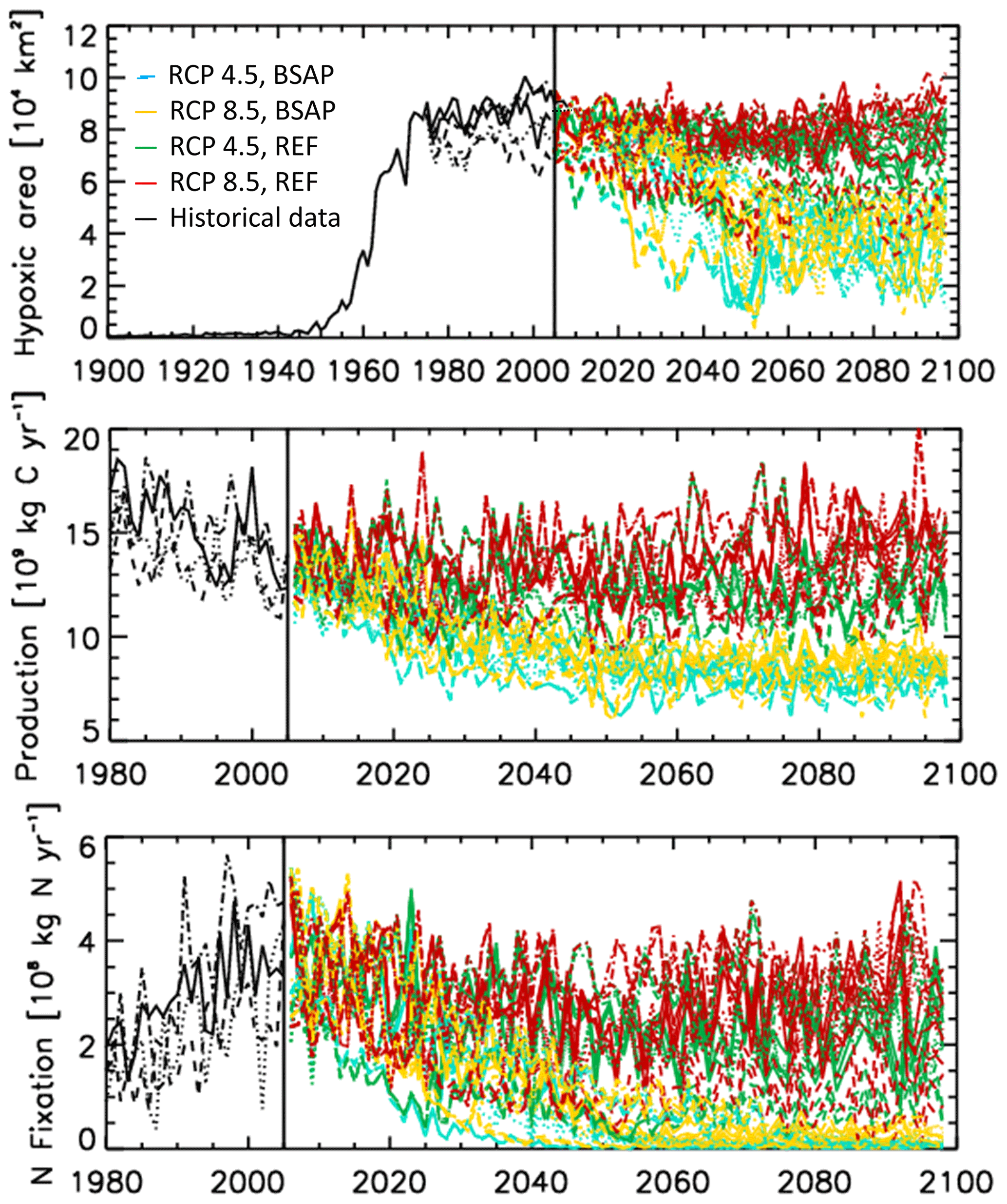
Figure 23From top to bottom: hypoxic area (in km2), volume-averaged primary production (in kg C yr−1) and volume-averaged nitrogen fixation (in kg N yr−1) for the entire Baltic Sea, including the Kattegat (see Fig. 1) in the historical (until 2005, black lines) and scenario (after 2005, coloured lines) simulations driven by four regionalised ESMs (illustrated by different line types) under RCP4.5, BSAP (blue), RCP4.5, REF (green), RCP8.5, BSAP (orange) and RCP8.5, REF (red) scenarios. A spin-up simulation since 1850 was performed, as illustrated by the evolution of hypoxia. (Source: Meier et al., 2021; their Fig. 4 distributed under the terms of the Creative Commons CC-BY 4.0 License, http://creativecommons.org/licenses/by/4.0/, last access: 6 January 2022.)
In accordance with previous studies, such as Saraiva et al. (2019b) and Meier et al. (2021), the impact of warming (reduced oxygen solubility, increased internal nutrient cycling, increased riverine inputs) and of increasing stratification (decreased ventilation) will be an amplified depletion of oxygen that enlarges the hypoxia area in the Baltic Sea and partially counteracts nutrient input abatement strategies such as the BSAP. However, in all available scenarios, the impact of climate change is smaller than the impact of nutrient input changes.
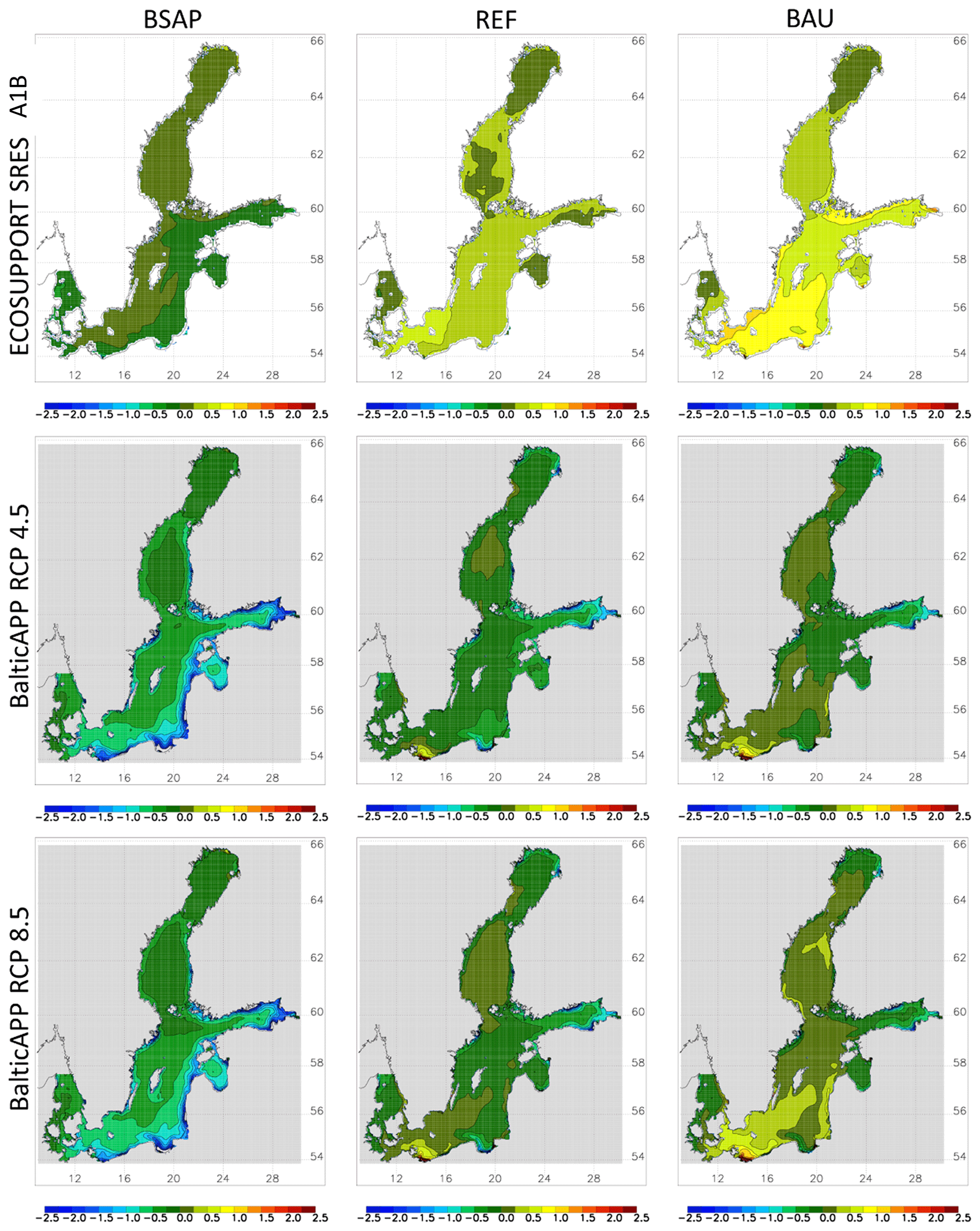
Figure 24As in Fig. 21 but for annual mean surface phytoplankton concentration changes (mg Chl m−3). Concentrations are vertically averaged for the upper 10 m. (Source: Meier et al., 2011b; Saraiva et al., 2019a.)
3.2.7 Nutrient concentrations
While in ECOSUPPORT scenario simulations of future climate the projected surface phosphate concentrations in winter increase under all three nutrient input scenarios (except in the Gulf of Finland in BSAP), in BalticAPP projections the surface phosphate concentrations in winter decrease almost everywhere (except in the Oder Bight and adjacent areas in REF and WORST) (not shown). In contrast to the nearly ubiquitous changes in the surface phosphate concentration, larger nitrate concentration changes are usually confined to the coastal zone and differ in their signs. In ECOSUPPORT projections, the increases in winter surface nitrate concentrations in REF and BAU are largest in the Gulf of Riga, the eastern Gulf of Finland and along the eastern coasts of the Baltic Proper (not shown). In BalticAPP projections, the increases in winter surface nitrate concentrations in REF and WORST are largest in the Bothnian Bay and the Odra Bight, while in the Gulf of Riga and the Vistula lagoon nitrate concentrations decrease. Overall, the differences in surface nutrient concentrations between the two sets of scenario simulations are considerable (not shown) and can be explained by the large differences in nutrient inputs from land. Thus, while the projected changes in inputs in ECOSUPPORT refer to the average inputs during 1995–2002, in BalticAPP scenario simulations the observed historical changes include a decline in nutrient inputs since the 1980s (Meier et al., 2018a).
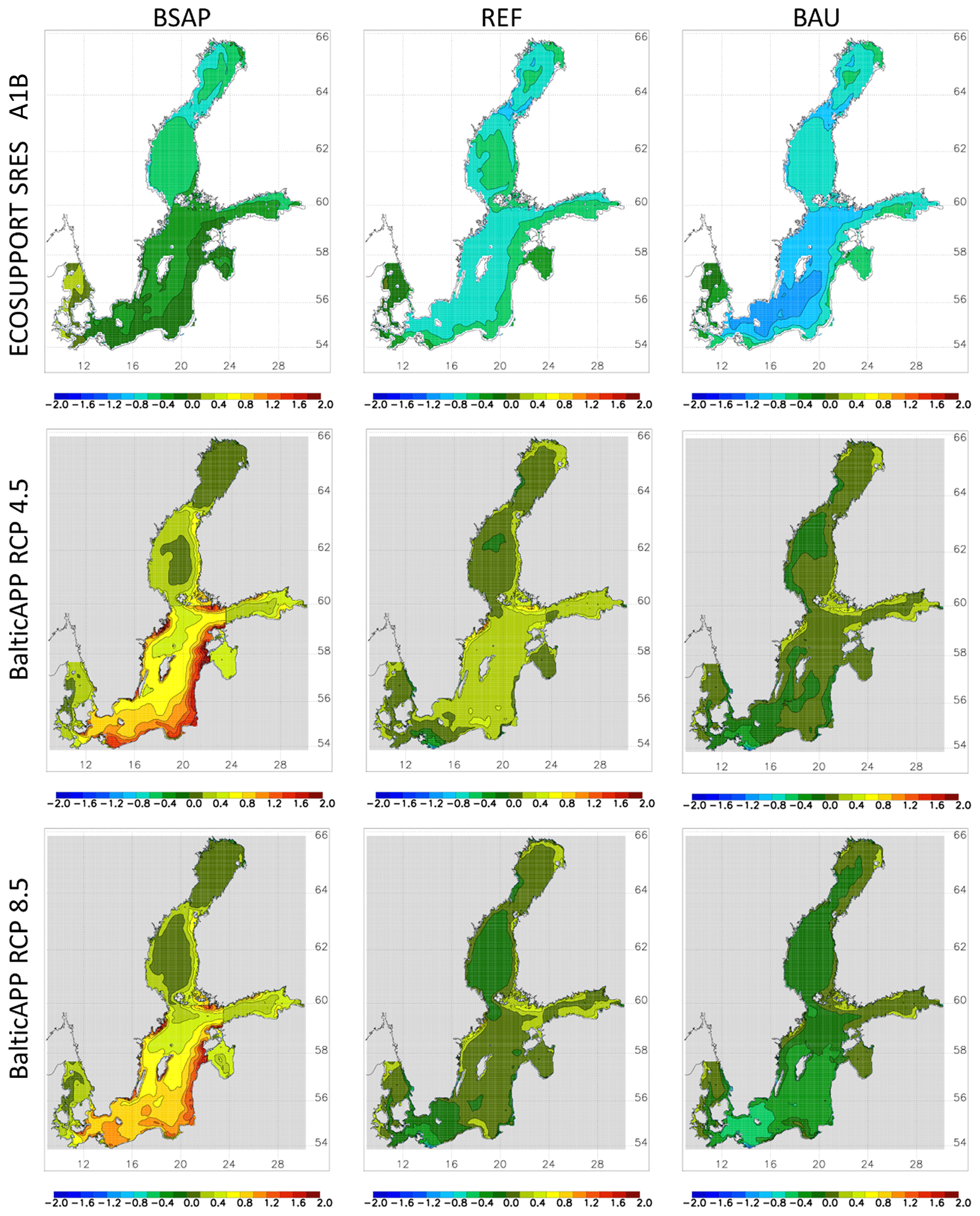
Figure 25As in Fig. 21 but for changes in the annual mean Secchi depth (m). (Source: Meier et al., 2011b; Saraiva et al., 2019a.)
3.2.8 Phytoplankton concentrations
Annual mean changes in surface phytoplankton concentration (expressed as chlorophyll concentration) follow the changes in nutrient concentrations and are confined to the productive zone along the coasts (Fig. 24). In ECOSUPPORT projections, annual mean Secchi depths decrease in all scenario simulations (see Fig. 25 and Table 11). In the BalticAPP projections, the area-averaged Secchi depths generally increase, except in the combined RCP8.5 and BAU scenario (Table 11), indicating a general improvement of the water quality in future compared to the present climate. The most striking changes occur in the BSAP scenario, in which the Secchi depth increases by up to 2 m in the coastal zone of the eastern Baltic Proper. Changes in stratification (illustrated by the differences between BalticAPP and CLIMSEA ensembles and between the CLIMSEA ensemble mean and high SLR scenarios) have only a minor impact on water transparency (Table 11). The overwhelming driver of the changes in the Secchi depth is the nutrient input scenario (illustrated by the differences between ECOSUPPORT and BalticAPP/CLIMSEA ensembles and highlighted by, in some cases, contradictory signs in the changes).
Table 11As in Table 8 but showing the ensemble mean changes in the annual Secchi depth (in m) in the ECOSUPPORT, BalticAPP RCP4.5, BalticAPP RCP8.5, CLIMSEA RCP4.5 and CLIMSEA RCP8.5 scenario simulations averaged for the Baltic Sea including the Kattegat. The projected changes depend on the nutrient input scenario: BSAP, REF, BAU or WORST. (Data sources: Meier et al., 2011b, 2021; Saraiva et al., 2019a.)
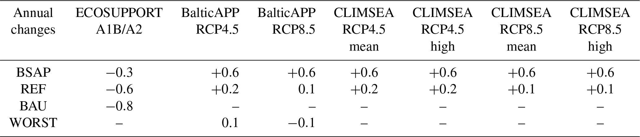
Figure 26Ensemble 10-year running mean North Atlantic Oscillation (NAO) index (a, b) and 10-year running correlation between the NAO and area-averaged SST in the Baltic Sea (c, d) under the RCP4.5 (a, c) and RCP8.5 (b, d) scenarios. Depicted are winter (December–February) mean, median, minimum, maximum and 15th and 85th percentiles. (Data source: Meier et al., 2021.)
3.2.9 Biogeochemical fluxes
In CLIMSEA under the BSAP, primary production and nitrogen fixation are projected to considerably decrease in a future climate (Fig. 23). According to this scenario, the interannual variability declines. Under REF, nitrogen fixation is projected to slightly decrease until ∼2050, as a delayed response to nutrient input reductions, and then to increase towards the end of the century, likely in response to increased nutrient inputs and warming. At the end of the century, primary production and nitrogen fixation will be at the same level as under current conditions. The impact of warming is larger under high than under low nutrient conditions (Saraiva et al., 2019b).
3.2.10 Relation to large-scale atmospheric circulation
The dominant large-scale atmospheric pattern controlling the climate in the Baltic Sea region during winter is the North Atlantic Oscillation (NAO; Hurrell, 1995). However, its influence is not stationary but depends on other modes of variability, such as the Atlantic Multidecadal Oscillation (AMO; Börgel et al., 2020). During the past climate, the relationship between the NAO index and regional climate variables in the Baltic Sea region, such as SST, changed over time (Vihma and Haapala, 2009; Omstedt and Chen, 2001; Hünicke and Zorita, 2006; Chen and Hellström, 1999; Meier and Kauker, 2002; Beranová and Huth, 2008).
Figure 26 shows the calculated ensemble mean winter (December–February) NAO index for the period 2006–2100. For the RCP4.5 emission scenario, the NAO shows high interannual variability. Following a wavelet analysis, the calculated NAO index exhibits decadal variability, which differs for every model (not shown). A comparison of RCP4.5 with the high-emission scenario RCP8.5 shows that the spread of the ensemble increases with increasing GHG concentrations. Figure 26 also depicts the running correlation between the NAO index and the area-averaged SST. The correlation remains positive but it is not constant in time. Also evident from a comparison of RCP4.5 and RCP8.5 is that there are no systematic changes in the two emission scenarios, although for RCP8.5 the ensemble spread is slightly larger.
In the largest set of scenario simulations of this study, the CLIMSEA ensemble, only four ESMs were regionalised using only one RCSM; consequently, this ensemble is still too small to estimate the uncertainties caused by ESM and RCSM differences. While nine ESMs with the same RCSM were recently regionalised, they did not include running modules for terrestrial and marine biogeochemistry (Gröger et al., 2021b), such that these simulations were not considered in our assessment. The uncertainties related to unresolved physical and biogeochemical processes in the Baltic Sea and on land were also not considered, because only one Baltic Sea and one catchment model were used. Although the CLIMSEA ensemble is larger than the ensembles in previous studies, it is still too small to estimate all sources of uncertainty.
In addition to the uncertainties related to global and regional climate and impact models, pathways of GHG and nutrient emissions are thus far unknown and the role of natural variability versus anthropogenic forcing is not well understood (Meier et al., 2018a, 2019b, 2021). Recent studies suggest that the impact of natural variability, such as the low-frequency AMO, is larger than hitherto estimated. For instance, in palaeoclimate simulations the AMO affected Baltic Sea salinity at timescales of 60–180 years (Börgel et al., 2018), which is longer than the simulation periods of available scenario simulations. Furthermore, the AMO may also influence the centres of action of the NAO (Börgel et al., 2020). Lateral tilting of the positions of the Icelandic Low and Azores High explains the changes in the correlations between the NAO and regional variables such as water temperature, sea-ice cover and river runoff in the Baltic Sea region (Börgel et al., 2020). Despite indications that the AMO is affected by climate states such as the Medieval Climate Anomaly and Little Ice Age (Wang et al., 2017; Börgel et al., 2018), how future warming would affect these modes of climate variability is unclear.
Changes in sea-ice cover were not analysed in this study because in the recent scenario simulations of the CLIMSEA ensemble sea-ice cover is systematically underestimated. However, we found that future sea-ice cover is projected to be considerably reduced, with an on-average ice-free Bothnian Sea and western Gulf of Finland. Recent results by Höglund et al. (2017) confirmed earlier results by Meier (2002b) and Meier et al. (2019d, 2014); see BACC Author Team (2008).
The various scenario simulation sets have in common that plausible nutrient input changes have a bigger impact on changes in biogeochemical variables, such as nutrient, phytoplankton and oxygen concentrations, than of either the projected changes in climate, such as warming, or changes in vertical stratification. The latter would be caused by increased freshwater inputs, SLR or changes in regional wind fields, assuming RCP4.5 or RCP8.5 scenarios. Long-term simulations of past climate support these results. Although historical warming had an impact on the size of the present-day hypoxic area, model results suggest that hypoxia in the Baltic Sea is best explained by the increases in nutrient inputs due to population growth and intensified agriculture since 1950 (Gustafsson et al., 2012; Carstensen et al., 2014; Meier et al., 2012a, 2019c, d). Hypoxia is also a feature of the Medieval Climate Anomaly (Zillén and Conley, 2010). However, a preliminary attempt to simulate the past 1000 years could not explain the low-oxygen conditions without substantial increases in nutrient inputs (Schimanke et al., 2012). Thus, the sensitivity of state-of-the-art physical–biogeochemical models to various drivers can be questioned and it is clear that the models do not reproduce all important processes.
As outlined in previous assessments, current and future bioavailable nutrient inputs from land and atmosphere are unknown and were consequently classified as one of the largest uncertainties (Meier et al., 2019b). For a more detailed discussion of uncertainties in Baltic Sea projections, the reader is referred to Meier et al. (2018a, 2019b, 2021).
As shown in Sect. 3, the latest published scenario simulations confirm the findings of the first and second assessments of climate change in the Baltic Sea region (BACC Author Team, 2008; BACC II Author Team, 2015), namely that, in all projections driven by RCP4.5 and RCP8.5 and by four selected ESMs of CMIP5, water temperature is projected to increase and sea-ice cover to decrease significantly. In the two RCP scenarios, the ensemble mean annual changes in SST between 1978–2007 and 2069–2098 are 2 and 3 ∘C, respectively. Warming would enhance the stability across the seasonal thermocline and cause a shallower MLD during summer. During winter, however, the mixed layer in the northern Baltic Sea would be deeper, probably because of the declining sea-ice cover and the associated intensification of wind speed, waves and vertical mixing. Both the frequency and the duration of MHWs would increase significantly, in particular south of 60∘ N and in the coastal zone (except in regions with frequent upwellings).
The spatial patterns of seasonal SST trends projected for 2006–2099 are similar to those of historical reconstructions of the period 1850–2008, although in most regions the magnitude of the simulated trends is larger. The largest trends are those in summer in the northern Baltic Sea (Bothnian Sea and Bothnian Bay) and thus in regions where under a warmer climate sea ice would melt earlier or disappear completely due to the ice–albedo feedback. This implies that, with increasing warming, SST trends in the northern Baltic Sea will become larger than those in the southern Baltic Sea. Accordingly, in contrast to the present climate, in which mean SSTs considerably decline from south to north, in a future climate the north–south temperature gradient will weaken.
In contrast to previous scenario simulations, recent scenario simulations considered the impact of the global mean SLR on Baltic Sea salinity, which for the ensemble mean salinity would more or less completely compensate for the effects of the projected increasing river runoff. However, as future changes in all three drivers of salinity (wind, runoff and SLR) are highly uncertain, the spread in the salinity projections of the various ESMs is larger than any signal.
In agreement with earlier assessments, we conclude that SLR has a greater potential to increase surge levels in the Baltic Sea than does changing wind speed or direction. For the latter, there have been no statistically significant changes during the 21st century thus far.
In agreement with earlier studies, changes in nutrient input according to the BSAP or REF scenarios will have a larger impact on biogeochemical cycling in the Baltic Sea than will a changing climate driven by RCP4.5 or RCP8.5 scenarios. Furthermore, the impact of climate change will be more pronounced under higher than under lower nutrient conditions. Hence, without further nutrient input reductions, as suggested by the BSAP, eutrophication and oxygen depletion will worsen. However, the response determined in recent studies differs considerably from the responses reported in previous studies, because of more plausible assumptions regarding historical and future nutrient inputs. In some cases, this has led to opposite signs in the response of bottom oxygen concentrations. The new scenarios suggest that implementation of the BSAP would lead to a significant improvement in the ecological status of the Baltic Sea regardless of the applied RCP scenario.
However, recent studies identified SLR as a new global driver. Depending on the combination of SLR and RCP scenarios, the impact on the bottom oxygen concentration may be significant. A higher mean sea level relative to the seabed at the sills would cause increased saltwater inflows, a stronger vertical stratification in the Baltic Sea and a larger hypoxic area. The relationship between vertical stratification and the size of the hypoxic area was confirmed in historical measurements. Nevertheless, recent studies suggest that the difference in future nutrient emissions between the BSAP and REF scenarios is a more important driver than the projected changes in climate with respect to changes in hypoxic area, phytoplankton concentration, water transparency (Secchi depth), primary production and nitrogen fixation.
The currently available ensembles of scenario simulations are larger than those in previous studies. Consequently, the uncertainty range covered by the assessed ESMs and, in turn, the spread of the results are also larger. However, the ensemble size might still be too small and model uncertainty is very likely underestimated. Moreover, natural variability might be a more important source of uncertainty than previously considered for applications in the Baltic Sea.
In the present climate, the climate variability of the Baltic Sea region during winter is dominated by the impact of the NAO. However, in the past, the correlation between the NAO and regional variables such as water temperature or sea ice varied in time. The low-frequency changes in this correlation are projected to continue. Furthermore, systematic changes in the influence of the large-scale atmospheric circulation on regional climate and on the NAO itself could not be detected. While a northward shift in the mean summer position of the westerlies at the end of the 21st century compared to the 20th century was reported (Gröger et al., 2019), it was based upon a limited set of simulations with a few ESMs.
This is a review article and no new data were generated. The sources of data displayed in the figures and tables have been cited. All data are publicly available.
HEMM designed the review article, coordinated the writing and produced the tables. Analyses of publicly available data resulting in additional figures were performed by MG, CD, KS, FB and HEMM. All authors contributed to the writing of the article with text and comments.
The contact author has declared that neither they nor their co-authors have any competing interests.
Publisher's note: Copernicus Publications remains neutral with regard to jurisdictional claims in published maps and institutional affiliations.
This article is part of the special issue “The Baltic Earth Assessment Reports (BEAR)”. It is not associated with a conference.
During the preparation of this paper, shortly before its submission, our co-author, Christian Dieterich, passed away (1964–2021). This sad event marked the end of the life of a distinguished oceanographer and climate scientist who made important contributions to climate modelling for the Baltic Sea, North Sea and North Atlantic regions.
This study belongs to the series of Baltic Earth Assessment Reports (BEAR) of the Baltic Earth Program (Earth System Science for the Baltic Sea Region; Baltic Earth, 2022) and is dedicated to Christian Dieterich. The work was financed by the Copernicus Marine Environment Monitoring Service through the CLIMSEA project (Regionally downscaled climate projections for the Baltic and North seas, CMEMS 66-SE-CALL2: LOT4) and by the Swedish Research Council for Environment, Agricultural Sciences and Spatial Planning (Formas) through the ClimeMarine project within the framework of the National Research Programme for Climate (grant no. 2017-01949). Regional climate scenario simulations were conducted on the Linux clusters Krypton, Bi, Triolith and Tetralith, all operated by the National Supercomputer Centre in Sweden (NSC, http://www.nsc.liu.se/, last access: 6 January 2022). Resources on Triolith and Tetralith were funded by the Swedish National Infrastructure for Computing (SNIC) (grant nos. SNIC 002/12-25, SNIC 2018/3-280 and SNIC 2019/3-356). Furthermore, we thank Berit Recklebe (Leibniz Institute for Baltic Sea Research Warnemünde, IOW) for technical support and Boris Chubarenko and Vladimir Ryabchenko for their very good comments that helped to improve an earlier version of the manuscript.
The work was financed by the Copernicus Marine Environment Monitoring Service through the CLIMSEA project (Regionally downscaled climate projections for the Baltic and North seas, CMEMS 66-SE-CALL2: LOT4) and by the Swedish Research Council for Environment, Agricultural Sciences and Spatial Planning (Formas) through the ClimeMarine project within the framework of the National Research Programme for Climate (grant no. 2017-01949). Regional climate scenario simulations were conducted on the Linux clusters Krypton, Bi, Triolith and Tetralith, all operated by the National Supercomputer Centre in Sweden (NSC, http://www.nsc.liu.se/, last access: 6 January 2022). Resources on Triolith and Tetralith were funded by the Swedish National Infrastructure for Computing (SNIC) (grant nos. SNIC 002/12-25, SNIC 2018/3-280 and SNIC 2019/3-356).
This paper was edited by Marcus Reckermann and reviewed by Vladimir Ryabchenko and Boris Chubarenko.
Almroth-Rosell, E., Eilola, K., Hordoir, R., Meier, H. E. M., and Hall, P. O. J.: Transport of fresh and resuspended particulate organic material in the Baltic Sea – a model study, J. Mar. Syst., 87, 1–12, https://doi.org/10.1016/j.jmarsys.2011.02.005, 2011.
Almroth-Rosell, E., Eilola, K., Kuznetsov, I., Hall, P. O. J., and Meier, H. E. M.: A new approach to model oxygen dependent benthic phosphate fluxes in the Baltic Sea, J. Mar. Syst., 144, 127–141, https://doi.org/10.1016/j.jmarsys.2014.11.007, 2015.
Arheimer, B., Dahné, J., and Donnelly, C.: Climate change impact on riverine nutrient load and land-based remedial measures of the Baltic Sea Action Plan, Ambio, 41, 600–612, https://doi.org/10.1007/s13280-012-0323-0, 2012.
BACC Author Team: Assessment of climate change for the Baltic Sea basin, in: Regional Climate Studies, Springer Science & Business Media, Berlin, Heidelberg, 473 pp., https://doi.org/10.1007/978-3-540-72786-6, 2008.
BACC II Author Team: Second Assessment of Climate Change for the Baltic Sea Basin, in: Regional Climate Studies, Springer International Publishing, Cham, https://doi.org/10.1007/978-3-319-16006-1, 2015.
Baltic Earth – Earth System Science for the Baltic Sea Region: Extending the knowledge of the regional Earth system in the Baltic Sea region, available at: https://baltic.earth/, last access: 6 January 2022.
Bamber, J. L., Oppenheimer, M., Kopp, R. E., Aspinall, W. P., and Cooke, R. M.: Ice sheet contributions to future sea-level rise from structured expert judgment, P. Natl. Acad. Sci. USA, 116, 11195, https://doi.org/10.1073/pnas.1817205116, 2019.
Bauer, B., Gustafsson, B. G., Hyytiäinen, K., Meier, H. E. M., Müller-Karulis, B., Saraiva, S., and Tomczak, M. T.: Food web and fisheries in the future Baltic Sea, Ambio, 48, 1337–1349, https://doi.org/10.1007/s13280-019-01229-3, 2019.
Belkin, I. M.: Rapid warming of large marine ecosystems, Prog. Oceanogr., 81, 207–213, https://doi.org/10.1016/j.pocean.2009.04.011, 2009.
Beranová, R. and Huth, R.: Time variations of the effects of circulation variability modes on European temperature and precipitation in winter, Int. J. Climatol., 28, 139–158, https://doi.org/10.1002/joc.1516, 2008.
Bergström, S. and Carlsson, B.: River runoff to the Baltic Sea – 1950–1990, Ambio, 23, 280–287, 1994.
Börgel, F., Frauen, C., Neumann, T., Schimanke, S., and Meier, H. E. M.: Impact of the Atlantic Multidecadal Oscillation on Baltic Sea Variability, Geophys. Res. Lett., 45, 9880–9888, https://doi.org/10.1029/2018GL078943, 2018.
Börgel, F., Frauen, C., Neumann, T., and Meier, H. E. M.: The Atlantic Multidecadal Oscillation controls the impact of the North Atlantic Oscillation on North European climate, Environ. Res. Lett., 15, 104025, https://doi.org/10.1088/1748-9326/aba925, 2020.
Bülow, K., Dietrich, C., Elizalde, A., Gröger, M., Heinrich, H., Hüttl-Kabos, S., Klein, B., Mayer, B., Meier, H. E. M., and Mikolajewicz, U.: Comparison of three regional coupled ocean atmosphere models for the North Sea under today's and future climate conditions (KLIWAS Schriftenreihe; KLIWAS-27/2014), Bundesanstalt für Gewässerkunde, 265 pp., available at: https://epic.awi.de/id/eprint/36453/ (last access: 6 January 2022), 2014.
Carstensen, J., Andersen, J. H., Gustafsson, B. G., and Conley, D. J.: Deoxygenation of the Baltic Sea during the last century, P. Natl. Acad. Sci. USA, 111, 5628–5633, https://doi.org/10.1073/pnas.1323156111, 2014.
Chen, D. and Hellström, C.: The influence of the North Atlantic Oscillation on the regional temperature variability in Sweden: spatial and temporal variations, Tellus A, 51, 505–516, https://doi.org/10.1034/j.1600-0870.1999.t01-4-00004.x, 1999.
Christensen, O. B., Kjellström, E., Dieterich, C., Gröger, M., and Meier, H. E. M.: Atmospheric regional climate projections for the Baltic Sea Region until 2100, Earth Syst. Dynam. Discuss. [preprint], https://doi.org/10.5194/esd-2021-51, in review, 2021.
Church, J. A., Clark, P. U., Cazenave, A., Gregory, J. M., Jevrejeva, S., Levermann, A., Merrifield, M. A., Milne, G. A., Nerem, R. S., Nunn, P. D., Payne, A. J., Pfeffer, W. T., Stammer, D., and Unnikrishnan, A. S.: Sea Level Change, in: Climate Change 2013 – The Physical Science Basis: Working Group I Contribution to the Fifth Assessment Report of the Intergovernmental Panel on Climate Change, edited by: Stocker, T. F., Qin, D., Plattner, G.-K., Tignor, M., Allen, S. K., Boschung, J., Nauels, A., Xia, Y., Bex, V., and Midgley, P. M., Cambridge University Press, Cambridge, UK, New York, USA, 1137–1216, https://doi.org/10.1017/CBO9781107415324, 2013.
de Boyer Montégut, C., Madec, G., Fischer, A. S., Lazar, A., and Iudicone, D.: Mixed layer depth over the global ocean: An examination of profile data and a profile-based climatology, J. Geophys. Res.-Oceans, 109, 109, C12003, https://doi.org/10.1029/2004jc002378, 2004.
Dieterich, C., Schimanke, S., Wang, S., Väli, G., Liu, Y., Hordoir, R., Höglund, A., and Meier, H. E. M.: Evaluation of the SMHI coupled atmosphere-ice-ocean model RCA4-NEMO, SMHI, Norrköping, Sweden, 80 pp., 2013.
Dieterich, C., Wang, S., Schimanke, S., Gröger, M., Klein, B., Hordoir, R., Samuelsson, P., Liu, Y., Axell, L., and Höglund, A.: Surface heat budget over the North Sea in climate change simulations, Atmosphere, 10, 272, https://doi.org/10.3390/atmos10050272, 2019.
Donnelly, C., Arheimer, B., Capell, R., Dahne, J., and Strömqvist, J.: Regional overview of nutrient load in Europe–challenges when using a large-scale model approach, E-HYPE, Proceedings of the H04, IAHS-IAPSO-IASPEI Assembly, 4, 49–58, 2013.
Donnelly, C., Greuell, W., Andersson, J., Gerten, D., Pisacane, G., Roudier, P., and Ludwig, F.: Impacts of climate change on European hydrology at 1.5, 2 and 3 degrees mean global warming above preindustrial level, Climatic Change, 143, 13–26, https://doi.org/10.1007/s10584-017-1971-7, 2017.
Döscher, R. and Meier, H. E. M.: Simulated sea surface temperature and heat fluxes in different climates of the Baltic Sea, Ambio, 33, 242–248, https://doi.org/10.1579/0044-7447-33.4.242, 2004.
Döscher, R., Willén, U., Jones, C., Rutgersson, A., Meier, H. E. M., Hansson, U., and Graham, L. P.: The development of the regional coupled ocean-atmosphere model RCAO, Boreal Environ. Res., 7, 183–192, 2002.
Dutheil, C., Meier, H. E. M., Gröger, M., and Börgel, F.: Understanding past and future sea surface temperature trends in the Baltic Sea, Clim. Dynam., https://doi.org/10.1007/s00382-021-06084-1, in press, 2021.
Ehrnsten, E., Norkko, A., Müller-Karulis, B., Gustafsson, E., and Gustafsson, B. G.: The meagre future of benthic fauna in a coastal sea – Benthic responses to recovery from eutrophication in a changing climate, Global Change Biol., 26, 2235–2250, https://doi.org/10.1111/gcb.15014, 2020.
Eilola, K., Meier, H. E. M., and Almroth, E.: On the dynamics of oxygen, phosphorus and cyanobacteria in the Baltic Sea; A model study, J. Mar. Syst., 75, 163–184, https://doi.org/10.1016/j.jmarsys.2008.08.009, 2009.
Eilola, K., Gustafsson, B. G., Kuznetsov, I., Meier, H. E. M., Neumann, T., and Savchuk, O. P.: Evaluation of biogeochemical cycles in an ensemble of three state-of-the-art numerical models of the Baltic Sea, J. Mar. Syst., 88, 267–284, https://doi.org/10.1016/j.jmarsys.2011.05.004, 2011.
Eilola, K., Mårtensson, S., and Meier, H. E. M.: Modeling the impact of reduced sea ice cover in future climate on the Baltic Sea biogeochemistry, Geophys. Res. Lett., 40, 149–154, https://doi.org/10.1029/2012GL054375, 2013.
Ekman, M. and Mäkinen, J.: Mean sea surface topography in the Baltic Sea and its transition area to the North Sea: A geodetic solution and comparisons with oceanographic models, J. Geophys. Res.-Oceans, 101, 11993–11999, https://doi.org/10.1029/96JC00318, 1996.
Feser, F., Rockel, B., von Storch, H., Winterfeldt, J., and Zahn, M.: Regional Climate Models Add Value to Global Model Data: A Review and Selected Examples, B. Am. Meteorol. Soc., 92, 1181–1192, https://doi.org/10.1175/2011BAMS3061.1, 2011.
Fleming-Lehtinen, V. and Laamanen, M.: Long-term changes in Secchi depth and the role of phytoplankton in explaining light attenuation in the Baltic Sea, Estuar. Coast. Shelf Sci., 102–103, 1–10, https://doi.org/10.1016/j.ecss.2012.02.015, 2012.
Fonselius, S. and Valderrama, J.: One hundred years of hydrographic measurements in the Baltic Sea, J. Sea Res., 49, 229–241, https://doi.org/10.1016/S1385-1101(03)00035-2, 2003.
Friedland, R., Neumann, T., and Schernewski, G.: Climate change and the Baltic Sea action plan: model simulations on the future of the western Baltic Sea, J. Mar. Syst., 105–108, 175–186, https://doi.org/10.1016/j.jmarsys.2012.08.002, 2012.
Friedland, R., Macias, D., Cossarini, G., Daewel, U., Estournel, C., Garcia-Gorriz, E., Grizzetti, B., Grégoire, M., Gustafson, B., Kalaroni, S., Kerimoglu, O., Lazzari, P., Lenhart, H., Lessin, G., Maljutenko, I., Miladinova, S., Müller-Karulis, B., Neumann, T., Pärn, O., Pätsch, J., Piroddi, C., Raudsepp, U., Schrum, C., Stegert, C., Stips, A., Tsiaras, K., Ulses, C., and Vandenbulcke, L.: Effects of nutrient management scenarios on marine eutrophication indicators: a Pan-European, multi-model assessment in support of the Marine Strategy Framework Directive, Front. Mar. Sci., 8, 596126, https://doi.org/10.3389/fmars.2021.596126, 2021.
Giorgi, F.: Simulation of Regional Climate Using a Limited Area Model Nested in a General Circulation Model, J. Climate, 3, 941–963, https://doi.org/10.1175/1520-0442(1990)003<0941:Sorcua>2.0.Co;2, 1990.
Giorgi, F. and Gao, X.-J.: Regional earth system modeling: review and future directions, Atmos. Ocean. Sci. Lett., 11, 189–197, https://doi.org/10.1080/16742834.2018.1452520, 2018.
Gogina, M., Zettler, M. L., Wåhlström, I., Andersson, H., Radtke, H., Kuznetsov, I., and MacKenzie, B. R.: A combination of species distribution and ocean-biogeochemical models suggests that climate change overrides eutrophication as the driver of future distributions of a key benthic crustacean in the estuarine ecosystem of the Baltic Sea, ICES J. Mar. Sci., 77, 2089–2105, https://doi.org/10.1093/icesjms/fsaa107, 2020.
Gordon, C., Cooper, C., Senior, C. A., Banks, H., Gregory, J. M., Johns, T. C., Mitchell, J. F. B., and Wood, R. A.: The simulation of SST, sea ice extents and ocean heat transports in a version of the Hadley Centre coupled model without flux adjustments, Clim. Dynam., 16, 147–168, https://doi.org/10.1007/s003820050010, 2000.
Gräwe, U. and Burchard, H.: Storm surges in the Western Baltic Sea: the present and a possible future, Clim. Dynam., 39, 165–183, https://doi.org/10.1007/s00382-011-1185-z, 2012.
Gräwe, U., Friedland, R., and Burchard, H.: The future of the western Baltic Sea: two possible scenarios, Ocean Dynam., 63, 901–921, https://doi.org/10.1007/s10236-013-0634-0, 2013.
Griffies, S. M.: Fundamentals of ocean climate models, Princeton University Press, Princeton, https://doi.org/10.1515/9780691187129, 2004.
Grinsted, A.: Projected Change – Sea Level, in: Second Assessment of Climate Change for the Baltic Sea Basin, in: Regional Climate Studies, edited by: BACC II Author Team, Springer International Publishing, Cham, 253–263, https://doi.org/10.1007/978-3-319-16006-1_14, 2015.
Gröger, M., Dieterich, C., Meier, H. E. M., and Schimanke, S.: Thermal air-sea coupling in hindcast simulations for the North Sea and Baltic Sea on the NW European shelf, Tellus A, 67, 26911, https://doi.org/10.3402/tellusa.v67.26911, 2015.
Gröger, M., Arneborg, L., Dieterich, C., Höglund, A., and Meier, H. E. M.: Summer hydrographic changes in the Baltic Sea, Kattegat and Skagerrak projected in an ensemble of climate scenarios downscaled with a coupled regional ocean–sea ice–atmosphere model, Clim. Dynam., 53, 5945–5966, https://doi.org/10.1007/s00382-019-04908-9, 2019.
Gröger, M., Dieterich, C., Haapala, J., Ho-Hagemann, H. T. M., Hagemann, S., Jakacki, J., May, W., Meier, H. E. M., Miller, P. A., Rutgersson, A., and Wu, L.: Coupled regional Earth system modeling in the Baltic Sea region, Earth Syst. Dynam., 12, 939–973, https://doi.org/10.5194/esd-12-939-2021, 2021a.
Gröger, M., Dieterich, C., and Meier, H. E. M.: Is interactive air sea coupling relevant for simulating the future climate of Europe?, Clim. Dynam., 56, 491–514, https://doi.org/10.1007/s00382-020-05489-8, 2021b.
Gustafsson, B. G., Savchuk, O. P., and Meier, H. E. M.: Load scenarios for ECOSUPPORT, Technical Report No. 4, Baltic Nest Institute, Stockholm, Sweden, 24 pp., 2011.
Gustafsson, B. G., Schenk, F., Blenckner, T., Eilola, K., Meier, H. E. M., Müller-Karulis, B., Neumann, T., Ruoho-Airola, T., Savchuk, O. P., and Zorita, E.: Reconstructing the development of Baltic Sea eutrophication 1850–2006, Ambio, 41, 534–548, https://doi.org/10.1007/s13280-012-0318-x, 2012.
Haapala, J., Meier, H. E. M., and Rinne, J.: Numerical investigations of future ice conditions in the Baltic Sea, Ambio, 30, 237–244, https://doi.org/10.1579/0044-7447-30.4.237, 2001.
Heavens, N. G., Ward, D. S., and Natalie, M. J.: Studying and projecting climate change with earth system models, Nat. Educ. Knowledge, 4, 4, 2013.
HELCOM: Towards a Baltic Sea unaffected by eutrophication – HELCOM Overview 2007, in: HELCOM Ministerial Meeting, Krakow, Poland, 35 pp., 2007.
HELCOM: Approaches and methods for eutrophication target settingin the Baltic Sea region, Baltic Sea Environment Proceedings No. 133, Helsinki, Finland, 138 pp., 2013a.
HELCOM: HELCOM Copenhagen Ministerial Declaration – Taking Further Action to Implement the Baltic Sea Action Plan – Reaching Good Environmental Statusfor a healthyBaltic Sea, in: HELCOM Ministrial Meeting, Copenhagen, Denmark, 2013b.
HELCOM: State of the Baltic Sea – Second HELCOM holistic assessment 2011–2016, Baltic Sea Environment Proceedings No. 155, Helsinki, Finland, 155 pp., 2018.
Hense, I. and Beckmann, A.: Towards a model of cyanobacteria life cycle – effects of growing and resting stages on bloom formation of N2-fixing species, Ecol. Model., 195, 205–218, https://doi.org/10.1016/j.ecolmodel.2005.11.018, 2006.
Hense, I., and Beckmann, A.: The representation of cyanobacteria life cycle processes in aquatic ecosystem models, Ecol. Model., 221, 2330–2338, https://doi.org/10.1016/j.ecolmodel.2010.06.014, 2010.
Hieronymus, J., Eilola, K., Olofsson, M., Hense, I., Meier, H. E. M., and Almroth-Rosell, E.: Modeling cyanobacteria life cycle dynamics and historical nitrogen fixation in the Baltic Proper, Biogeosciences, 18, 6213–6227, https://doi.org/10.5194/bg-18-6213-2021, 2021.
Hieronymus, M. and Kalén, O.: Sea-level rise projections for Sweden based on the new IPCC special report: The ocean and cryosphere in a changing climate, Ambio, 49, 1587–1600, https://doi.org/10.1007/s13280-019-01313-8, 2020.
Hill, E. M., Davis, J. L., Tamisiea, M. E., and Lidberg, M.: Combination of geodetic observations and models for glacial isostatic adjustment fields in Fennoscandia, J. Geophys. Res.-Solid, 115, B07403, https://doi.org/10.1029/2009jb006967, 2010.
Hobday, A. J., Oliver, E. C. J., Gupta, A. S., Benthuysen, J. A., Burrows, M. T., Donat, M. G., Holbrook, N. J., Moore, P. J., Thomsen, M. S., Wernberg, T., and Smale, D. A.: Categorizing and Naming MARINE HEATWAVES, Oceanography, 31, 162–173, 2018.
Höglund, A., Pemberton, P., Hordoir, R., and Schimanke, S.: Ice conditions for maritime traffic in the Baltic Sea in future climate, Boreal Environ. Res., 22, 245–265, 2017.
Holopainen, R., Lehtiniemi, M., Meier, H. E. M., Albertsson, J., Gorokhova, E., Kotta, J., and Viitasalo, M.: Impacts of changing climate on the non-indigenous invertebrates in the northern Baltic Sea by end of the twenty-first century, Biol. Invas., 18, 3015–3032, https://doi.org/10.1007/s10530-016-1197-z, 2016.
Holt, J., Schrum, C., Cannaby, H., Daewel, U., Allen, I., Artioli, Y., Bopp, L., Butenschon, M., Fach, B. A., Harle, J., Pushpadas, D., Salihoglu, B., and Wakelin, S.: Potential impacts of climate change on the primary production of regional seas: A comparative analysis of five European seas, Prog. Oceanogr., 140, 91–115, https://doi.org/10.1016/j.pocean.2015.11.004, 2016.
Hordoir, R. and Meier, H. E. M.: Effect of climate change on the thermal stratification of the baltic sea: a sensitivity experiment, Clim. Dynam., 38, 1703–1713, https://doi.org/10.1007/s00382-011-1036-y, 2012.
Hordoir, R., Höglund, A., Pemberton, P., and Schimanke, S.: Sensitivity of the overturning circulation of the Baltic Sea to climate change, a numerical experiment, Clim. Dynam., 50, 1425–1437, https://doi.org/10.1007/s00382-017-3695-9, 2018.
Hordoir, R., Axell, L., Höglund, A., Dieterich, C., Fransner, F., Gröger, M., Liu, Y., Pemberton, P., Schimanke, S., Andersson, H., Ljungemyr, P., Nygren, P., Falahat, S., Nord, A., Jönsson, A., Lake, I., Döös, K., Hieronymus, M., Dietze, H., Löptien, U., Kuznetsov, I., Westerlund, A., Tuomi, L., and Haapala, J.: Nemo-Nordic 1.0: a NEMO-based ocean model for the Baltic and North seas – research and operational applications, Geosci. Model Dev., 12, 363–386, https://doi.org/10.5194/gmd-12-363-2019, 2019.
Hundecha, Y., Arheimer, B., Donnelly, C., and Pechlivanidis, I.: A regional parameter estimation scheme for a pan-European multi-basin model, J. Hydrol.: Reg. Stud., 6, 90–111, https://doi.org/10.1016/j.ejrh.2016.04.002, 2016.
Hünicke, B. and Zorita, E.: Influence of temperature and precipitation on decadal Baltic Sea level variations in the 20th century, Tellus A, 58, 141–153, https://doi.org/10.1111/j.1600-0870.2006.00157.x, 2006.
Hünicke, B., Zorita, E., Soomere, T., Madsen, K. S., Johansson, M., and Suursaar, Ü.: Recent Change – Sea Level and Wind Waves, in: Second Assessment of Climate Change for the Baltic Sea Basin, edited by: BACC II Author Team, Springer International Publishing, Cham, 155–185, https://doi.org/10.1007/978-3-319-16006-1_9, 2015.
Hurrell, J. W.: Decadal trends in the North Atlantic Oscillation: regional temperatures and precipitation, Science-AAAS-Weekly Paper Edition, 269, 676–679, https://doi.org/10.1126/science.269.5224.676, 1995.
IPCC: Climate Change 2013 – The Physical Science Basis: Working Group I Contribution to the Fifth Assessment Report of the Intergovernmental Panel on Climate Change, https://doi.org/10.1017/CBO9781107415324, 2013.
IPCC: IPCC Special Report on the Ocean and Cryosphere in a Changing Climate, edited by: Pörtner, H.-O., Roberts, D. C., Masson-Delmotte, V., Zhai, P., Tignor, M., Poloczanska, E., Mintenbeck, K., Alegría, A., Nicolai, M., Okem, A., Petzold, J., Rama, B., and Weyer, N. M., IPCC, available at: https://www.ipcc.ch/site/assets/uploads/sites/3/2019/12/SROCC_Citations.pdf (last access: 6 January 2022), 2019a.
IPCC: Summary for Policymakers, in: IPCC Special Report on the Ocean and Cryosphere in a Changing Climate, edited by: Pörtner, H.-O., Roberts, D. C., Masson-Delmotte, V., Zhai, P., Tignor, M., Poloczanska, E., Mintenbeck, K., Alegría, A., Nicolai, M., Okem, A., Petzold, J., Rama, B., and Weyer, N. M., IPCC, available at: https://www.ipcc.ch/site/assets/uploads/sites/3/2019/12/SROCC_Citations.pdf (last access: 6 January 2022), 2019b.
IPCC: Climate Change 2021: The Physical Science Basis, in: Contribution of Working Group I to the Sixth Assessment Report of the Intergovernmental Panel on Climate Change, edited by: Masson-Delmotte, V., Zhai, P., Pirani, A., Connors, S. L., Péan, C., Berger, S., Caud, N., Chen, Y., Goldfarb, L., Gomis, M. I., Huang, M., Leitzell, K., Lonnoy, E., Matthews, J. B. R., Maycock, T. K., Waterfield, T., Yelekçi, O., Yu, R., and Zhou, B., Cambridge University Press, Cambridge, available at: https://www.ipcc.ch/ (last access: 22 January 2022), 2021.
Jacob, D., Petersen, J., Eggert, B., Alias, A., Christensen, O. B., Bouwer, L. M., Braun, A., Colette, A., Déqué, M., Georgievski, G., Georgopoulou, E., Gobiet, A., Menut, L., Nikulin, G., Haensler, A., Hempelmann, N., Jones, C., Keuler, K., Kovats, S., Kröner, N., Kotlarski, S., Kriegsmann, A., Martin, E., v. Meijgaard, E., Moseley, C., Pfeifer, S., Preuschmann, S., Radermacher, C., Radtke, K., Rechid, D., Rounsevell, M., Samuelsson, P., Somot, S., Soussana, J.-F., Teichmann, C., Valentini, R., Vautard, R., Weber, B., and Yiou, P.: EURO-CORDEX: new high-resolution climate change projections for European impact research, Reg. Environ. Change, 14, 563–578, https://doi.org/10.1007/s10113-013-0499-2, 2014.
Jungclaus, J. H., Keenlyside, N., Botzet, M., Haak, H., Luo, J.-J., Latif, M., Marotzke, J., Mikolajewicz, U., and Roeckner, E.: Ocean circulation and tropical variability in the coupled model ECHAM5/MPI-OM, J. Climate, 19, 3952–3972, https://doi.org/10.1175/JCLI3827.1, 2006.
Jutterström, S., Andersson, H. C., Omstedt, A., and Malmaeus, J. M.: Multiple stressors threatening the future of the Baltic Sea – Kattegat marine ecosystem: Implications for policy and management actions, Mar. Pollut. Bull., 86, 468–480, https://doi.org/10.1016/j.marpolbul.2014.06.027, 2014.
Kniebusch, M., Meier, H. E. M., Neumann, T., and Börgel, F.: Temperature Variability of the Baltic Sea Since 1850 and Attribution to Atmospheric Forcing Variables, J. Geophys. Res.-Oceans, 124, 4168–4187, https://doi.org/10.1029/2018jc013948, 2019.
Knight, J. R., Allan, R. J., Folland, C. K., Vellinga, M., and Mann, M. E.: A signature of persistent natural thermohaline circulation cycles in observed climate, Geophys. Res. Lett., 32, L20708, https://doi.org/10.1029/2005gl024233, 2005.
Kotilainen, A. T., Arppe, L., Dobosz, S., Jansen, E., Kabel, K., Karhu, J., Kotilainen, M. M., Kuijpers, A., Lougheed, B. C., Meier, H. E. M., Moros, M., Neumann, T., Porsche, C., Poulsen, N., Rasmussen, P., Ribeiro, S., Risebrobakken, B., Ryabchuk, D., Schimanke, S., Snowball, I., Spiridonov, M., Virtasalo, J. J., Weckström, K., Witkowski, A., and Zhamoida, V.: Echoes from the Past: A Healthy Baltic Sea Requires More Effort, Ambio 43, 60–68, https://doi.org/10.1007/s13280-013-0477-4, 2014.
Kratzer, S., Håkansson, B., and Charlotte, S.: Assessing Secchi and Photic Zone Depth in the Baltic Sea from Satellite Data, Ambio, 32, 577–585, 2003.
Kupiainen, M., Jansson, C., Samuelsson, P., Jones, C., Willén, U., Hansson, U., Ullerstig, A., Wang, S., and Döscher, R.: Rossby Centre regional atmospheric model, RCA4, Rossby Center News Letter, SMHI, Norrköping, Sweden, 2014.
Kuznetsov, I. and Neumann, T.: Simulation of carbon dynamics in the Baltic Sea with a 3D model, J. Mar. Syst., 111–112, 167–174, https://doi.org/10.1016/j.jmarsys.2012.10.011, 2013.
Lang, A. and Mikolajewicz, U.: The long-term variability of extreme sea levels in the German Bight, Ocean Sci., 15, 651–668, https://doi.org/10.5194/os-15-651-2019, 2019.
Lehmann, A., Getzlaff, K., and Harlaß, J.: Detailed assessment of climate variability in the Baltic Sea area for the period 1958 to 2009, Clim. Res., 46, 185–196, https://doi.org/10.3354/cr00876, 2011.
Liu, Y., Meier, H. E. M., and Eilola, K.: Nutrient transports in the Baltic Sea – results from a 30-year physical–biogeochemical reanalysis, Biogeosciences, 14, 2113–2131, https://doi.org/10.5194/bg-14-2113-2017, 2017.
MacKenzie, B. R., Meier, H. E. M., Lindegren, M., Neuenfeldt, S., Eero, M., Blenckner, T., Tomczak, M. T., and Niiranen, S.: Impact of Climate Change on Fish Population Dynamics in the Baltic Sea: A Dynamical Downscaling Investigation, Ambio 41, 626–636, https://doi.org/10.1007/s13280-012-0325-y, 2012.
Madec, G. and the NEMO team: NEMO ocean engine, version 3.6 stable, Note du Pôle de modélisation de l'Institut Pierre-Simon Laplace (IPSL) No. 27, France, 396 pp., available at: https://www.nemo-ocean.eu/wp-content/uploads/NEMO_book.pdf (last access: 6 January 2022), 2016.
Madsen, K. S., Høyer, J. L., Suursaar, Ü., She, J., and Knudsen, P.: Sea Level Trends and Variability of the Baltic Sea From 2D Statistical Reconstruction and Altimetry, Front. Earth Sci., 7, 243, https://doi.org/10.3389/feart.2019.00243, 2019.
Meehl, G. A., Washington, W. M., Ammann, C. M., Arblaster, J. M., Wigley, T. M. L., and Tebaldi, C.: Combinations of Natural and Anthropogenic Forcings in Twentieth-Century Climate, J. Climate, 17, 3721–3727, https://doi.org/10.1175/1520-0442(2004)017<3721:conaaf>2.0.co;2, 2004.
Meier, H. E. M.: On the parameterization of mixing in three-dimensional Baltic Sea models, J. Geophys. Res.-Oceans, 106, 30997–31016, https://doi.org/10.1029/2000JC000631, 2001.
Meier, H. E. M.: Regional ocean climate simulations with a 3D ice–ocean model for the Baltic Sea. Part 2: results for sea ice, Clim. Dynam., 19, 255–266, https://doi.org/10.1007/s00382-001-0225-5, 2002a.
Meier, H. E. M.: Regional ocean climate simulations with a 3D ice-ocean model for the Baltic Sea. Part 1: model experiments and results for temperature and salinity, Clim. Dynam., 19, 237–253, https://doi.org/10.1007/s00382-001-0224-6, 2002b.
Meier, H. E. M.: Baltic Sea climate in the late twenty-first century: a dynamical downscaling approach using two global models and two emission scenarios, Clim. Dynam., 27, 39–68, https://doi.org/10.1007/s00382-006-0124-x, 2006.
Meier, H. E. M.: Modeling the pathways and ages of inflowing salt-and freshwater in the Baltic Sea, Estuar. Coast. Shelf Sci., 74, 610–627, https://doi.org/10.1016/j.ecss.2007.05.019, 2007.
Meier, H. E. M. and Kauker, F.: Simulating Baltic Sea climate for the period 1902–1998 with the Rossby Centre coupled ice-ocean model, SMHI, Norrköping, Sweden, 2002.
Meier, H. E. M. and Kauker, F.: Modeling decadal variability of the Baltic Sea: 2. Role of freshwater inflow and large-scale atmospheric circulation for salinity, J. Geophys. Res.-Oceans, 108, 3368, https://doi.org/10.1029/2003JC001799, 2003.
Meier, H. E. M. and Saraiva, S.: Projected Oceanographical Changes in the Baltic Sea until 2100, Oxford Research Encyclopedia of Climate Science, https://doi.org/10.1093/acrefore/9780190228620.013.699, 2020.
Meier, H. E. M., Doescher, R., Coward, A. C., Nycander, J., and Döös, K.: RCO – Rossby Centre regional Ocean climate model: model description (version 1.0) and first results from the hindcast period 1992/93, SMHI, Norrköping, Sweden, 102 pp., 1999.
Meier, H. E. M., Döscher, R., and Faxén, T.: A multiprocessor coupled ice-ocean model for the Baltic Sea: Application to salt inflow, J. Geophys. Res.-Oceans, 108, 3273, https://doi.org/10.1029/2000JC000521, 2003.
Meier, H. E. M., Broman, B., and Kjellström, E.: Simulated sea level in past and future climates of the Baltic Sea, Clim. Res., 27, 59–75, https://doi.org/10.3354/cr027059, 2004a.
Meier, H. E. M., Döscher, R., and Halkka, A.: Simulated distributions of Baltic Sea-ice in warming climate and consequences for the winter habitat of the Baltic ringed seal, Ambio, 33, 249–256, https://doi.org/10.1579/0044-7447-33.4.249, 2004b.
Meier, H. E. M., Kjellström, E., and Graham, L. P.: Estimating uncertainties of projected Baltic Sea salinity in the late 21st century, Geophys. Res. Lett., 33, L15705, https://doi.org/10.1029/2006GL026488, 2006.
Meier, H. E. M., Andersson, H., Dieterich, C., Eilola, K., Gustafsson, B., Höglund, A., and Schimanke, S.: Transient scenario simulations for the Baltic Sea Region during the 21st century, SMHI, Norrköping, Sweden, 81 pp., 2011a.
Meier, H. E. M., Andersson, H. C., Eilola, K., Gustafsson, B. G., Kuznetsov, I., Müller-Karulis, B., Neumann, T., and Savchuk, O. P.: Hypoxia in future climates: A model ensemble study for the Baltic Sea, Geophys. Res. Lett., 38, L24608, https://doi.org/10.1029/2011GL049929, 2011b.
Meier, H. E. M., Eilola, K., and Almroth, E.: Climate-related changes in marine ecosystems simulated with a 3-dimensional coupled physical-biogeochemical model of the Baltic Sea, Clim. Res., 48, 31–55, https://doi.org/10.3354/cr00968, 2011c.
Meier, H. E. M., Höglund, A., Döscher, R., Andersson, H., Löptien, U., and Kjellström, E.: Quality assessment of atmospheric surface fields over the Baltic Sea from an ensemble of regional climate model simulations with respect to ocean dynamics, Oceanologia, 53, 193–227, https://doi.org/10.5697/oc.53-1-TI.193, 2011d.
Meier, H. E. M., Andersson, H. C., Arheimer, B., Blenckner, T., Chubarenko, B., Donnelly, C., Eilola, K., Gustafsson, B. G., Hansson, A., Havenhand, J., Höglund, A., Kuznetsov, I., MacKenzie, B. R., Müller-Karulis, B., Neumann, T., Niiranen, S., Piwowarczyk, J., Raudsepp, U., Reckermann, M., Ruoho-Airola, T., Savchuk, O. P., Schenk, F., Schimanke, S., Väli, G., Weslawski, J.-M., and Zorita, E.: Comparing reconstructed past variations and future projections of the Baltic Sea ecosystem – first results from multi-model ensemble simulations, Environ. Res. Lett., 7, 34005, https://doi.org/10.1088/1748-9326/7/3/034005, 2012a.
Meier, H. E. M., Eilola, K., Gustavsson, B. G., Kuznetsov, I., Neumann, T., and Savchuk, O. P.: Uncertainty assessment of projected ecological quality indicators in future climate, SMHI, Norrköping, Sweden, 2012b.
Meier, H. E. M., Hordoir, R., Andersson, H. C., Dieterich, C., Eilola, K., Gustafsson, B. G., Höglund, A., and Schimanke, S.: Modeling the combined impact of changing climate and changing nutrient loads on the Baltic Sea environment in an ensemble of transient simulations for 1961–2099, Clim. Dynam., 39, 2421–2441, https://doi.org/10.1007/s00382-012-1339-7, 2012c.
Meier, H. E. M., Müller-Karulis, B., Andersson, H. C., Dieterich, C., Eilola, K., Gustafsson, B. G., Höglund, A., Hordoir, R., Kuznetsov, I., Neumann, T., Ranjbar, Z., Savchuk, O. P., and Schimanke, S.: Impact of climate change on ecological quality indicators and biogeochemical fluxes in the Baltic Sea: a multi-model ensemble study, Ambio, 41, 558-573, https://doi.org/10.1007/s13280-012-0320-3, 2012d.
Meier, H. E. M., Andersson, H. C., Arheimer, B., Donnelly, C., Eilola, K., Gustafsson, B. G., Kotwicki, L., Neset, T.-S., Niiranen, S., Piwowarczyk, J., Savchuk, O. P., Schenk, F., Weslawski, J. M., and Zorita, E.: Ensemble modeling of the Baltic Sea ecosystem to provide scenarios for management, Ambio, 43, 37–48, https://doi.org/10.1007/s13280-013-0475-6, 2014.
Meier, H. E. M., Höglund, A., Eilola, K., and Almroth-Rosell, E.: Impact of accelerated future global mean sea level rise on hypoxia in the Baltic Sea, Clim. Dynam., 49, 163–172, https://doi.org/10.1007/s00382-016-3333-y, 2017.
Meier, H. E. M., Edman, M. K., Eilola, K. J., Placke, M., Neumann, T., Andersson, H. C., Brunnabend, S.-E., Dieterich, C., Frauen, C., Friedland, R., Gröger, M., Gustafsson, B. G., Gustafsson, E., Isaev, A., Kniebusch, M., Kuznetsov, I., Müller-Karulis, B., Omstedt, A., Ryabchenko, V., Saraiva, S., and Savchuk, O. P.: Assessment of Eutrophication Abatement Scenarios for the Baltic Sea by Multi-Model Ensemble Simulations, Front. Mar. Sci., 5, 440, https://doi.org/10.3389/fmars.2018.00440, 2018a.
Meier, H. E. M., Väli, G., Naumann, M., Eilola, K., and Frauen, C.: Recently accelerated oxygen consumption rates amplify deoxygenation in the Baltic Sea, J. Geophys. Res.-Oceans, 123, 3227–3240, https://doi.org/10.1029/2017JC013686, 2018b.
Meier, H. E. M., Dieterich, C., Eilola, K., Gröger, M., Höglund, A., Radtke, H., Saraiva, S., and Wåhlström, I.: Future projections of record-breaking sea surface temperature and cyanobacteria bloom events in the Baltic Sea, Ambio, 48, 1362–1376, https://doi.org/10.1007/s13280-019-01235-5, 2019a.
Meier, H. E. M., Edman, M., Eilola, K., Placke, M., Neumann, T., Andersson, H. C., Brunnabend, S.-E., Dieterich, C., Frauen, C., Friedland, R., Gröger, M., Gustafsson, B. G., Gustafsson, E., Isaev, A., Kniebusch, M., Kuznetsov, I., Müller-Karulis, B., Naumann, M., Omstedt, A., Ryabchenko, V., Saraiva, S., and Savchuk, O. P.: Assessment of Uncertainties in Scenario Simulations of Biogeochemical Cycles in the Baltic Sea, Front. Mar. Sci., 6, 46, https://doi.org/10.3389/fmars.2019.00046, 2019b.
Meier, H. E. M., Eilola, K., Almroth-Rosell, E., Schimanke, S., Kniebusch, M., Höglund, A., Pemberton, P., Liu, Y., Väli, G., and Saraiva, S.: Correction to: Disentangling the impact of nutrient load and climate changes on Baltic Sea hypoxia and eutrophication since 1850, Clim. Dynam., 53, 1167–1169, https://doi.org/10.1007/s00382-018-4483-x, 2019c.
Meier, H. E. M., Eilola, K., Almroth-Rosell, E., Schimanke, S., Kniebusch, M., Höglund, A., Pemberton, P., Liu, Y., Väli, G., and Saraiva, S.: Disentangling the impact of nutrient load and climate changes on Baltic Sea hypoxia and eutrophication since 1850, Clim. Dynam., 53, 1145–1166, https://doi.org/10.1007/s00382-018-4296-y, 2019d.
Meier, H. E. M., Dieterich, C., and Gröger, M.: Natural variability is a large source of uncertainty in future projections of hypoxia in the Baltic Sea, Commun. Earth Environ., 2, 50, https://doi.org/10.1038/s43247-021-00115-9, 2021.
Mohrholz, V.: Major Baltic Inflow Statistics – Revised, Front. Mar. Sci., 5, 384, https://doi.org/10.3389/fmars.2018.00384, 2018.
Moss, R. H., Edmonds, J. A., Hibbard, K. A., Manning, M. R., Rose, S. K., v. Vuuren, D. P., Carter, T. R., Emori, S., Kainuma, M., Kram, T., Meehl, G. A., Mitchell, J. F. B., Nakicenovic, N., Riahi, K., Smith, S. J., Stouffer, R. J., Thomson, A. M., Weyant, J. P., and Wilbanks, T. J.: The next generation of scenarios for climate change research and assessment, Nature, 463, 747–756, https://doi.org/10.1038/nature08823, 2010.
Nakicenovic, N., Alcamo, J., Grubler, A., Riahi, K., Roehrl, R. A., Rogner, H.-H., and Victor, N.: Special report on emissions scenarios (SRES), a special report of Working Group III of the intergovernmental panel on climate change, IPCC Special Report, ISBN 92-9169-113-5, 2000.
Neumann, T.: Climate-change effects on the Baltic Sea ecosystem: A model study, J. Mar. Syst., 81, 213–224, https://doi.org/10.1016/j.jmarsys.2009.12.001, 2010.
Neumann, T., Eilola, K., Gustafsson, B., Müller-Karulis, B., Kuznetsov, I., Meier, H. E. M., and Savchuk, O. P.: Extremes of temperature, oxygen and blooms in the Baltic Sea in a changing climate, Ambio, 41, 574–585, https://doi.org/10.1007/s13280-012-0321-2, 2012.
Niiranen, S., Yletyinen, J., Tomczak, M. T., Blenckner, T., Hjerne, O., MacKenzie, B. R., Müller-Karulis, B., Neumann, T., and Meier, H. E. M.: Combined effects of global climate change and regional ecosystem drivers on an exploited marine food web, Global Change Biol., 19, 3327–3342, https://doi.org/10.1111/gcb.12309, 2013.
Omstedt, A. and Chen, D.: Influence of atmospheric circulation on the maximum ice extent in the Baltic Sea, J. Geophys. Res.-Oceans, 106, 4493–4500, https://doi.org/10.1029/1999JC000173, 2001.
Omstedt, A., Gustafsson, B., Rodhe, J., and Walin, G.: Use of Baltic Sea modelling to investigate the water cycle and the heat balance in GCM and regional climate models, Clim. Res., 15, 95–108, https://doi.org/10.3354/cr015095, 2000.
Omstedt, A., Edman, M., Claremar, B., Frodin, P., Gustafsson, E., Humborg, C., Hägg, H., Mörth, M., Rutgersson, A., Schurgers, G., Smith, B., Wällstedt, T., and Yurova, A.: Future changes in the Baltic Sea acid–base (pH) and oxygen balances, Tellus B, 64, 19586, https://doi.org/10.3402/tellusb.v64i0.19586, 2012.
Omstedt, A., Humborg, C., Pempkowiak, J., Perttilä, M., Rutgersson, A., Schneider, B., and Smith, B.: Biogeochemical control of the coupled CO2–O2 system of the Baltic Sea: a review of the results of Baltic-C, Ambio, 43, 49–59, https://doi.org/10.1007/s13280-013-0485-4, 2014.
Oppenheimer, M., Glavovic, B. C., Hinkel, J., v. d. Wal, R., Magnan, A. K., Abd-Elgawad, A., Cai, R., Cifuentes-Jara, M., DeConto, R. M., Ghosh, T., Hay, J., Isla, F., Marzeion, B., Meyssignac, B., and Sebesvari, Z.: Sea Level Rise and Implications for Low-Lying Islands, Coasts and Communities, in: IPCC Special Report on the Ocean and Cryosphere in a Changing Climate, edited by: Pörtner, H.-O., Roberts, D. C., Masson-Delmotte, V., Zhai, P., Tignor, M., Poloczanska, E., Mintenbeck, K., Alegría, A., Nicolai, M., Okem, A., Petzold, J., Rama, B., and Weyer, N. M., available at: https://www.ipcc.ch/site/assets/uploads/sites/3/2019/12/SROCC_Citations.pdf (last access: 6 January 2022), 2019.
Pellikka, H., Särkkä, J., Johansson, M., and Pettersson, H.: Probability distributions for mean sea level and storm contribution up to 2100 AD at Forsmark, Technical Report TR-19-23, SKB – Swedish Nuclear Fuel and Waste Management Company, 49 pp., 2020.
Pihlainen, S., Zandersen, M., Hyytiäinen, K., Andersen, H. E., Bartosova, A., Gustafsson, B., Jabloun, M., McCrackin, M., Meier, H. E. M., Olesen, J. E., Saraiva, S., Swaney, D., and Thodsen, H.: Impacts of changing society and climate on nutrient loading to the Baltic Sea, Sci. Total Environ., 138935, https://doi.org/10.1016/j.scitotenv.2020.138935, 2020.
Placke, M., Meier, H. E. M., Gräwe, U., Neumann, T., Frauen, C., and Liu, Y.: Long-Term Mean Circulation of the Baltic Sea as Represented by Various Ocean Circulation Models, Front. Mar. Sci., 5, 287, https://doi.org/10.3389/fmars.2018.00287, 2018.
Placke, M., Meier, H. E. M., and Neumann, T.: Sensitivity of the Baltic Sea Overturning Circulation to Long-Term Atmospheric and Hydrological Changes, J. Geophys. Res.-Oceans, 126, e2020JC016079, https://doi.org/10.1029/2020JC016079, 2021.
Pushpadas, D., Schrum, C., and Daewel, U.: Projected climate change impacts on North Sea and Baltic Sea: CMIP3 and CMIP5 model based scenarios, Biogeosciences Discuss., 12, 12229–12279, https://doi.org/10.5194/bgd-12-12229-2015, 2015.
Quante, M. and Colijn, F.: North Sea region climate change assessment, in: Regional Climate Studies, SpringerOpen, Cham, https://doi.org/10.1007/978-3-319-39745-0, 2016.
Räisänen, J., Hansson, U., Ullerstig, A., Döscher, R., Graham, L. P., Jones, C., Meier, H. E. M., Samuelsson, P., and Willén, U.: European climate in the late twenty-first century: regional simulations with two driving global models and two forcing scenarios, Clim. Dynam., 22, 13–31, https://doi.org/10.1007/s00382-003-0365-x, 2004.
Reckermann, M., Omstedt, A., Soomere, T., Aigars, J., Akhtar, N., Bełdowska, M., Bełdowski, J., Cronin, T., Czub, M., Eero, M., Hyytiäinen, K. P., Jalkanen, J.-P., Kiessling, A., Kjellström, E., Kuliński, K., Larsén, X. G., McCrackin, M., Meier, H. E. M., Oberbeckmann, S., Parnell, K., Pons-Seres de Brauwer, C., Poska, A., Saarinen, J., Szymczycha, B., Undeman, E., Wörman, A., and Zorita, E.: Human impacts and their interactions in the Baltic Sea region, Earth Syst. Dynam., 13, 1–80, https://doi.org/10.5194/esd-13-1-2022, 2022.
Rockel, B.: The regional downscaling approach: a brief history and recent advances, Curr. Clim. Change Rep., 1, 22–29, https://doi.org/10.1007/s40641-014-0001-3, 2015.
Roeckner, E., Brokopf, R., Esch, M., Giorgetta, M., Hagemann, S., Kornblueh, L., Manzini, E., Schlese, U., and Schulzweida, U.: Sensitivity of simulated climate to horizontal and vertical resolution in the ECHAM5 atmosphere model, J. Climate, 19, 3771–3791, https://doi.org/10.1175/JCLI3824.1, 2006.
Rummukainen, M.: State-of-the-art with regional climate models, Wires Clim. Change, 1, 82–96, https://doi.org/10.1002/wcc.8, 2010.
Rummukainen, M.: Added value in regional climate modeling, Wires Clim. Change, 7, 145–159, https://doi.org/10.1002/wcc.378, 2016.
Rummukainen, M., Bergström, S., Persson, G., Rodhe, J., and Tjernström, M.: The Swedish Regional Climate Modelling Programme, SWECLIM: A Review, Ambio, 33, 176–182, 2004.
Rummukainen, M., Rockel, B., Bärring, L., Christensen, J. H., and Reckermann, M.: Twenty-first-century challenges in regional climate modeling, B. Am. Meteorol. Soc., 96, ES135–ES138, https://doi.org/10.1175/BAMS-D-14-00214.1, 2015.
Rutgersson, A., Jaagus, J., Schenk, F., Stendel, M., Bärring, L., Briede, A., ClaremarInger, B., Hanssen-Bauer, Holopainen, J., Moberg, A., Nordli, Ø., Rimkus, E., and Wibig, J.: Recent Change – Atmosphere, in: Second Assessment of Climate Change for the Baltic Sea Basin, edited by: BACC II Author Team, Regional Climate Studies, Springer International Publishing, Cham, 69–97, https://doi.org/10.1007/978-3-319-16006-1_4, 2015.
Ryabchenko, V. A., Karlin, L. N., Isaev, A. V., Vankevich, R. E., Eremina, T. R., Molchanov, M. S., and Savchuk, O. P.: Model estimates of the eutrophication of the Baltic Sea in the contemporary and future climate, Oceanology, 56, 36–45, https://doi.org/10.1134/S0001437016010161, 2016.
Samuelsson, P., Jones, C. G., Willén, U., Ullerstig, A., Gollvik, S., Hansson, U. L. F., Jansson, C., Kjellström, E., Nikulin, G., and Wyser, K.: The Rossby Centre Regional Climate model RCA3: model description and performance, Tellus A, 63, 4–23, https://doi.org/10.1111/j.1600-0870.2010.00478.x, 2011.
Saraiva, S., Meier, H. E. M., Andersson, H., Höglund, A., Dieterich, C., Gröger, M., Hordoir, R., and Eilola, K.: Uncertainties in Projections of the Baltic Sea Ecosystem Driven by an Ensemble of Global Climate Models, Front. Earth Sci., 6, 244, https://doi.org/10.3389/feart.2018.00244, 2019a.
Saraiva, S., Meier, H. E. M., Andersson, H., Höglund, A., Dieterich, C., Gröger, M., Hordoir, R., and Eilola, K.: Baltic Sea ecosystem response to various nutrient load scenarios in present and future climates, Clim. Dynam., 52, 3369–3387, https://doi.org/10.1007/s00382-018-4330-0, 2019b.
Savchuk, O. P., Larsson, U., and Elmgren, L.: Secchi depth and nutrient concentration in the Baltic Sea: model regressions for MARE's Nest, Version 2, Technical Report, Department of Systems Ecology, Stockholm University, Stockholm, Sweden, 12 pp., 2006.
Schimanke, S., Meier, H. E. M., Kjellström, E., Strandberg, G., and Hordoir, R.: The climate in the Baltic Sea region during the last millennium simulated with a regional climate model, Clim. Past, 8, 1419–1433, https://doi.org/10.5194/cp-8-1419-2012, 2012.
Schimanke, S. and Meier, H. E. M.: Decadal-to-Centennial Variability of Salinity in the Baltic Sea, J. Climate, 29, 7173–7188, https://doi.org/10.1175/JCLI-D-15-0443.1, 2016.
Schrum, C.: Regional Climate Modeling and Air-Sea Coupling, Oxford Research Encyclopedia of Climate Science, Oxford University Press, https://doi.org/10.1093/acrefore/9780190228620.013.3, 2017.
Schrum, C., Lowe, J., Meier, H. E. M., Grabemann, I., Holt, J., Mathis, M., Pohlmann, T., Skogen, M. D., Sterl, A., and Wakelin, S.: Projected Change – North Sea, in: North Sea Region Climate Change Assessment, edited by: Quante, M. and Colijn, F., SpringerOpen, Cham, 175–217, https://doi.org/10.1007/978-3-319-39745-0_6, 2016.
Sen, P. K.: Estimates of the Regression Coefficient Based on Kendall's Tau, J. Am. Stat. Assoc., 63, 1379–1389, https://doi.org/10.1080/01621459.1968.10480934, 1968.
Sjöberg, B.: Sea and coast, National atlas of Sweden, Almqvist and Wiksell International, Stockholm, Sweden, ISBN 9789187760167, 1992.
Skogen, M. D., Eilola, K., Hansen, J. L. S., Meier, H. E. M., Molchanov, M. S., and Ryabchenko, V. A.: Eutrophication status of the North Sea, Skagerrak, Kattegat and the Baltic Sea in present and future climates: A model study, J. Mar. Syst., 132, 174–184, https://doi.org/10.1016/j.jmarsys.2014.02.004, 2014.
Suursaar, Ü.: Combined impact of summer heat waves and coastal upwelling in the Baltic Sea, Oceanologia, 62, 511–524, https://doi.org/10.1016/j.oceano.2020.08.003, 2020.
Suursaar, Ü. and Sooäär, J.: Decadal variations in mean and extreme sea level values along the Estonian coast of the Baltic Sea, Tellus A, 59, 249–260, https://doi.org/10.1111/j.1600-0870.2006.00220.x, 2007.
Taylor, K. E., Stouffer, R. J., and Meehl, G. A.: An Overview of CMIP5 and the Experiment Design, B. Am. Meteorol. Soc., 93, 485–498, https://doi.org/10.1175/BAMS-D-11-00094.1, 2012.
Theil, H.: A rank-invariant method of linear and polynomial regression analysis, 3, Indagat. Math., 1, 1397–1412, 1950.
Uppala, S. M., KÅllberg, P. W., Simmons, A. J., Andrae, U., Bechtold, V. D. C., Fiorino, M., Gibson, J. K., Haseler, J., Hernandez, A., Kelly, G. A., Li, X., Onogi, K., Saarinen, S., Sokka, N., Allan, R. P., Andersson, E., Arpe, K., Balmaseda, M. A., Beljaars, A. C. M., Berg, L. V. D., Bidlot, J., Bormann, N., Caires, S., Chevallier, F., Dethof, A., Dragosavac, M., Fisher, M., Fuentes, M., Hagemann, S., Hólm, E., Hoskins, B. J., Isaksen, L., Janssen, P. A. E. M., Jenne, R., Mcnally, A. P., Mahfouf, J.-F., Morcrette, J.-J., Rayner, N. A., Saunders, R. W., Simon, P., Sterl, A., Trenberth, K. E., Untch, A., Vasiljevic, D., Viterbo, P., and Woollen, J.: The ERA-40 re-analysis, Q. J. Roy. Meteorol. Soc., 131, 2961–3012, https://doi.org/10.1256/qj.04.176, 2005.
van Vuuren, D. P., Edmonds, J., Kainuma, M., Riahi, K., Thomson, A., Hibbard, K., Hurtt, G. C., Kram, T., Krey, V., Lamarque, J.-F., Masui, T., Meinshausen, M., Nakicenovic, N., Smith, S. J., and Rose, S. K.: The representative concentration pathways: an overview, Climatic Change, 109, 5–31, https://doi.org/10.1007/s10584-011-0148-z, 2011.
Vihma, T. and Haapala, J.: Geophysics of sea ice in the Baltic Sea: A review, Prog. Oceanogr., 80, 129–148, https://doi.org/10.1016/j.pocean.2009.02.002, 2009.
Vuorinen, I., Hänninen, J., Rajasilta, M., Laine, P., Eklund, J., Montesino-Pouzols, F., Corona, F., Junker, K., Meier, H. E. M., and Dippner, J. W.: Scenario simulations of future salinity and ecological consequences in the Baltic Sea and adjacent North Sea areas – implications for environmental monitoring, Ecol. Indic., 50, 196–205, https://doi.org/10.1016/j.ecolind.2014.10.019, 2015.
Wang, J., Yang, B., Ljungqvist, F. C., Luterbacher, J., Osborn, Timothy, J., Briffa, K. R., and Zorita, E.: Internal and external forcing of multidecadal Atlantic climate variability over the past 1,200 years, Nat. Geosci., 10, 512–517, https://doi.org/10.1038/ngeo2962, 2017.
Wang, S., Dieterich, C., Döscher, R., Höglund, A., Hordoir, R., Meier, H. E. M., Samuelsson, P., and Schimanke, S.: Development and evaluation of a new regional coupled atmosphere–ocean model in the North Sea and Baltic Sea, Tellus A, 67, 24284, https://doi.org/10.3402/tellusa.v67.24284, 2015.
Weigel, B., Andersson, H. C., Meier, H. E. M., Blenckner, T., Snickars, M., and Bonsdorff, E.: Long-term progression and drivers of coastal zoobenthos in a changing system, Mar. Ecol. Prog. Ser., 528, 141–159, https://doi.org/10.3354/meps11279, 2015.
Weisse, R. and Hünicke, B.: Baltic Sea Level: Past, Present, and Future, Oxford Research Encyclopedia of Climate Science, Oxford University Press, https://doi.org/10.1093/acrefore/9780190228620.013.693, 2019.
Zandersen, M., Hyytiäinen, K., Meier, H. E. M., Tomczak, M. T., Bauer, B., Haapasaari, P. E., Olesen, J. E., Gustafsson, B. G., Refsgaard, J. C., Fridell, E., Pihlainen, S., Le Tissier, M. D. A., Kosenius, A.-K., and Van Vuuren, D. P.: Shared socio-economic pathways extended for the Baltic Sea: exploring long-term environmental problems, Reg. Environ. Change, 19, 1073–1086, https://doi.org/10.1007/s10113-018-1453-0, 2019.
Zillén, L. and Conley, D. J.: Hypoxia and cyanobacteria blooms – are they really natural features of the late Holocene history of the Baltic Sea?, Biogeosciences, 7, 2567–2580, https://doi.org/10.5194/bg-7-2567-2010, 2010.
https://helcom.fi/helcom-at-work/events/events-2021/ccfs-launch/ (last access: 6 January 2022).
One of the scenario simulations of ECOSUPPORT is driven by the A2 scenario, which due to higher GHG emissions is generally warmer than the A1B scenario. However, this particular simulation of the ECHAM5/MPIOM GCM is exceptional and at the end of the 21st century the temperature is not much warmer than that obtained with the corresponding run based on the same model under the A1B scenario.