the Creative Commons Attribution 4.0 License.
the Creative Commons Attribution 4.0 License.
 | 28 Oct 2022
Exploring the relationship between temperature forecast errors and Earth system variables
Melissa Ruiz-Vásquez
Sungmin O
Alexander Brenning
Randal D. Koster
Gianpaolo Balsamo
Ulrich Weber
Gabriele Arduini
Ana Bastos
Markus Reichstein
René Orth
Accurate subseasonal weather forecasts, from 2 weeks up to a season, can help reduce costs and impacts related to weather and corresponding extremes. The quality of weather forecasts has improved considerably in recent decades as models represent more details of physical processes, and they benefit from assimilating comprehensive Earth observation data as well as increasing computing power. However, with ever-growing model complexity, it becomes increasingly difficult to pinpoint weaknesses in the forecast models' process representations which is key to improving forecast accuracy. In this study, we use a comprehensive set of observation-based ecological, hydrological, and meteorological variables to study their potential for explaining temperature forecast errors at the weekly timescale. For this purpose, we compute Spearman correlations between each considered variable and the forecast error obtained from the European Centre for Medium-Range Weather Forecasts (ECMWF) subseasonal-to-seasonal (S2S) reforecasts at lead times of 1–6 weeks. This is done across the globe for the time period 2001–2017. The results show that temperature forecast errors globally are most strongly related with climate-related variables such as surface solar radiation and precipitation, which highlights the model's difficulties in accurately capturing the evolution of the climate-related variables during the forecasting period. At the same time, we find particular regions in which other variables are more strongly related to forecast errors. For instance, in central Europe, eastern North America and southeastern Asia, vegetation greenness and soil moisture are relevant, while in western South America and central North America, circulation-related variables such as surface pressure relate more strongly with forecast errors. Overall, the identified relationships between forecast errors and independent Earth observations reveal promising variables on which future forecasting system development could focus by specifically considering related process representations and data assimilation.
- Article
(12430 KB) - Full-text XML
-
Supplement
(1578 KB) - BibTeX
- EndNote


Forecasts at the subseasonal-to-seasonal timescale (S2S) have received growing attention in recent years (Kirtman et al., 2014; Vitart et al., 2017; White et al., 2017). Accurate predictions at the S2S are helpful, for instance, to anticipate extreme events like droughts and floods up to 2 weeks ahead (Bauer et al., 2015; Mariotti et al., 2018; Vitart and Robertson, 2018; Pegion et al., 2019; Pendergrass et al., 2020) and to optimize resource management (Robertson et al., 2015; White et al., 2017). The S2S bridges the gap between weather forecasts for the coming 2 weeks and seasonal climate predictions (Vitart, 2014; Robertson et al., 2015). However, it is particularly challenging to predict because the lead time is too long for the initial atmospheric conditions to provide useful information, and too short for some slowly varying Earth system components, such as the ocean, to effectively inform the forecasts (Vitart, 2014; Mariotti et al., 2018).
The chaotic nonlinear interactions between Earth system components and the uncertainties in the initial boundary conditions play a role in forecast errors (Newman et al., 2003). Forecasting systems need to capture all possible Earth system sources of subseasonal predictability to minimize these errors (Vitart and Robertson, 2018; de Andrade et al., 2019). The assimilation of climate variables, such as radiation and precipitation, and hence the representation of energy and water supply at the Earth's surface, is relevant to inform the weather forecast model to make accurate predictions of the evolution of temperature (Miller et al., 2021). This requires a global and dense observational network of respective measurements and/or regular satellite observations as a basis for an adequate data assimilation.
Related with climate variables, recent studies have identified potential circulation sources of S2S predictability such as Madden–Julian Oscillation (MJO), El Niño–Southern Oscillation (ENSO), and North Atlantic Oscillation (NAO). Atmospheric circulation patterns influence synoptic weather regimes and high/low pressure systems, which in turn modulate large-scale weather several weeks ahead (Büeler et al., 2021; Falkena et al., 2022).
Also, the land surface initial conditions (e.g., soil moisture, vegetation states, snow cover) contribute to subseasonal predictability through the memory, i.e., persistence in time, of related quantities, particularly in the case of soil moisture (Koster et al., 2010b, a; Saha et al., 2014; Mariotti et al., 2020; Kim et al., 2021; Meehl et al., 2021). Soil moisture can affect the partitioning of incoming radiation energy to sensible and latent heat fluxes, and therefore the near-surface temperature and humidity (Seneviratne et al., 2010). Soil moisture anomalies that are present and known at forecast initialization can persist for several weeks (Orth and Seneviratne, 2012; Shin et al., 2020), therefore an accurate representation of the soil moisture effect on surface heat fluxes supports weather forecast skill, particularly in water-limited regions (Miralles et al., 2012; Dirmeyer and Halder, 2017).
In contrast to soil moisture, the potential of vegetation phenology in improving weather forecast skills is not yet fully exploited, and in most forecasting systems, only the seasonal cycle is prescribed (Boussetta et al., 2013; Balsamo et al., 2018). Vegetation phenology (in terms of e.g., greenness and photosynthesis) affects surface heat fluxes through evapotranspiration, and exhibits memory. Some studies have outlined the potential of taking into account initial vegetation anomalies in the forecasting systems (Boussetta et al., 2015; Koster and Walker, 2015; Nogueira et al., 2020). They reveal the potential of the vegetation state in predicting hydrometeorological variables with high accuracy, especially during extreme events such as droughts and heat waves, permitting mitigation of their impacts (Meng et al., 2014; Albergel et al., 2019; Miralles et al., 2019).
Overall, these potential sources of forecast skill at the subseasonal timescale can vary in strength across space and time, and they are utilized to different degrees in current forecasting systems. Therefore, it is not obvious which is the most promising source of forecast skill to further exploit in forecasting system development. To provide guidance in this context, we study the temporal co-variability of errors of near-surface temperature forecasts with a comprehensive dataset of observation-based Earth system variables representing potentially under-exploited sources of forecast skill at the subseasonal timescale. With this setup, our goal is to reveal where (across regions) and when (across seasons) climate, circulation, and land surface variables can explain forecast error variability.
Our methodology is summarized in Fig. 1, and described in more detail in the following subsections.

Figure 1Schematic summary of the workflow. Within each grid cell, we calculate weekly averages of temperature forecast errors (lead times 1–6 weeks) and then compute their Spearman correlations with Earth system variables averaged across the week prior to the forecast start.
2.1 Data
Our analysis focuses on S2S reforecasts of 2 m air temperatures from the European Centre for Medium-Range Weather Forecasts (ECMWF) (Vitart et al., 2017), hereafter referred to as forecast. We use the average of 51 global ensemble members that differ with respect to (i) initial conditions (reflecting uncertainties in the data assimilation), and (ii) model parameterizations (reflecting modeling uncertainties). We consider the global land area and the period 2001–2017. Each forecast is run until a lead time of 46 d. We use forecasts generated in 2020 with two model versions: CY46R1 (all forecasts from 4 February to 29 June of each year) and CY47R1 (all forecasts from 30 June to 3 February of each year) (https://apps.ecmwf.int/datasets/data/s2s/, last access: 3 February 2021). There are no differences between the two model versions which have the potential to affect our results. The forecasts are forced with atmospheric data from the ERA5 reanalysis (Hersbach et al., 2020) and therefore benefit from a consistent model initialization.
All analyses in this study are performed on a weekly scale given the temporal resolution of the employed Earth system datasets and to minimize the effect of synoptic weather variability, following previous studies (Orth and Seneviratne, 2014; Koster et al., 2020). Consequently, the daily forecasts are aggregated to the weekly timescale by averaging forecast days 1–7 (week 1), 8–14 (week 2), 15–21 (week 3), 22–28 (week 4), 29–35 (week 5), and 36–42 (week 6).
In order to estimate errors in the temperature forecasts we compare them with respective data from the Climate Prediction Center (CPC) (https://psl.noaa.gov/data/gridded/data.cpc.globaltemp.html, last access: 21 December 2021). These data are model-independent and derived through interpolation of station observations. We calculate daily mean surface air temperatures as the average of each day's maximum and minimum temperatures, as recommended on the CPC website.
To assess the relationships of temperature forecast errors with multiple Earth system variables, we use the comprehensive set of data described in Table 1. A total of 21 variables are selected based on (i) literature about sources of predictability in seasonal forecasts, and (ii) physical processes and quantities which can affect surface air temperature. According to the Earth system component they are associated with, we classify these variables into three groups: climate, circulation, and land surface.
Trenberth (1997)Mo (2000)NOAA National Centers for Environmental Information (2017)NASA EOSDIS Land Processes DAAC (2015a)Jung et al. (2019)O and Orth (2021)
All datasets cover the entire globe and are linearly aggregated to a spatial resolution of in case this is not their native resolution, following a 2-dimensional piecewise linear interpolation method (Barber et al., 1996). In addition to considering absolute values of all variables listed in Table 1, we also consider their anomalies in our analysis of relationships with temperature forecast errors, except for the circulation indices ENSO, MJO, NAO, AAO, AO, and PNA which already come as anomalies. To compute anomalies we (i) subtract the long-term trend from each variable's time series, which we infer through a Lowess smoothing filter fit, and (ii) we remove the mean seasonal cycle, calculated at weekly time steps. Therefore, our final set of Earth system variables contains 36 variables (15 variables with both absolute values and anomalies, plus 6 circulation indices that are already anomalies).
We furthermore filter the vegetation-related Earth system variables in the land surface group (enhanced vegetation index (EVI), albedo, evaporative fraction) to include only sufficiently active vegetation (and hence evapotranspiration) that may physically affect temperatures (Seneviratne et al., 2010; Miralles et al., 2012). For this purpose, we do not consider grid cells nor weeks with EVI lower than 0.3 or temperatures below 10 ∘C.
2.2 Forecast error
We compute the weekly temperature forecast errors using an unbiased difference metric (Yu et al., 2006; McDonnell et al., 2018) between ECMWF–S2S temperature forecasts and CPC observational reference values, as shown in Eq. (1). Thereby, at each grid cell, (i) we compute the seasonal cycle as the climatological temperature of each week of the year, based on the 2001–2017 period, for the forecast and reference, respectively; (ii) we subtract the respective seasonal cycles from the temperature forecasts and the reference temperatures; and finally (iii) we compute the difference between the de-seasonalized forecast and reference temperatures.
where errori is the forecast error in the ith week; and are the climatological weekly temperature values (week-of-year averages) from the forecast and reference datasets, respectively; and Ti,for and Ti,ref are the forecast and reference temperature values respectively in the ith week.
The contributing stations of the reference temperature dataset are not uniformly distributed across the globe (Fig. A1). In our analysis, we omit grid cells without nearby stations as they can potentially exhibit larger interpolation errors. This way, we only consider grid cells with at least one temperature station located within the grid cell or in one of its eight neighboring grid cells. We assess and analyze the temperature forecast errors separately for each season, December–January–February (DJF), March–April–May (MAM), June–July–August (JJA), and September–October–November (SON), such that for each grid cell and season we consider weekly data across 3 months per season and 17 years, resulting in approximately 220 weeks per season.
2.3 Relating temperature forecast errors to Earth system variable dynamics
Our hypothesis is that a high temporal correlation between temperature forecast errors and any of the Earth system variables (Table 1) would indicate that the Earth system process represented by the respective variable is not yet sufficiently exploited by the forecasting system. We use the Spearman rank correlation coefficient (Wilks, 2011) to measure the strength of the relationship between forecast errors and each considered Earth system variable. This metric is chosen to account for potentially nonlinear relationships. It is calculated with Earth system variables averaged over the week prior to the forecast initialization and temperature forecast errors at lead times between 1 to 6 weeks, respectively. This way, we calculate correlation values for each of the 36 considered variables and for each weekly lead time, grid cell, and season. Finally we determine the highest correlation among them (in absolute terms), which indicates the most relevant Earth system variable and consequently the most promising information source to further improve temperature forecasts. Our interpretation focuses on the relevance of variables at the level of the aforementioned groups (climate, circulation, land surface).
We only consider correlations which are significant at the 5 % level. To infer significance in the light of the multiple testing at global scale (36 correlation values for the 36 Earth system variables across the globe), we perform the Benjamini–Hochberg procedure (Benjamini and Hochberg, 1995) to ensure control of the false discovery rate (Farcomeni, 2008; Cortés et al., 2020) by applying a correspondingly lower significance level. Additionally, we randomly permute the time series of each Earth system variable and compute their individual Spearman correlation values with forecast errors to compare their magnitude with our results.
Even though we analyze all weekly lead times (1 to 6), we focus on the lead time week 3 throughout most of the results section because this lead time represents well the subseasonal timescale (Brunet et al., 2010; Vitart et al., 2017; Pegion et al., 2019), which is less understood than the weather and climate scales (White et al., 2017). We find that the results after the lead time week 3 do not vary substantially.
We note a potential caveat in our approach due to existing relationships among our selected set of Earth system variables. Accordingly, we compute individual Spearman correlations among the 36 variables to account for the magnitude of these associations and to identify the most affected variables.
2.4 Case study: forecast errors in focus regions
We select six focus regions across all continents to further analyze the relationship between the temperature forecast errors and the respective most relevant Earth system variable. The regions are named according to the most relevant variables: specific humidity (sq), evaporative fraction (ef), total precipitation (tp), surface soil moisture (sm surf), meridional surface pressure differences (meridional sp), and ENSO (enso). We choose the regions to reflect clusters of grid cells with the same determined most important variable, and to represent different continents and Earth system variable groups. Table 2 displays the specific location of the six regions and their land cover classification from the MCD12C1 MODIS/Terra+Aqua land cover type dataset V006 (NASA EOSDIS Land Processes DAAC, 2015c).

2.5 Potential to improve temperature forecasts at the S2S timescale
Finally, we compute a measure of the potential to improve temperature forecasts in week 3 based on percentiles of (i) forecast errors and (ii) Spearman correlations of these errors with the most relevant Earth system variable identified in Sect. 3.2. Regions that exceed the 90th percentile for both quantities (forecast error and correlation values) have relatively large errors which at the same time can be attributed to an Earth system variable such that we determine this as the highest potential for improvement. For medium and low potential. the grid cell values need to exceed the 70th and 50th percentiles of all global grid cells, respectively.
3.1 Forecast error variability
At first we analyze the temperature forecast errors as reflected by the unbiased differences between the forecasted temperature and the reference data (Fig. 2). The largest mean seasonal errors occur during DJF with negative or positive biases depending on the region. We suggest that the biases in predicting temperatures are a consequence of imperfect model physics, initial conditions, and boundary conditions (Durai and Bhradwaj, 2014).
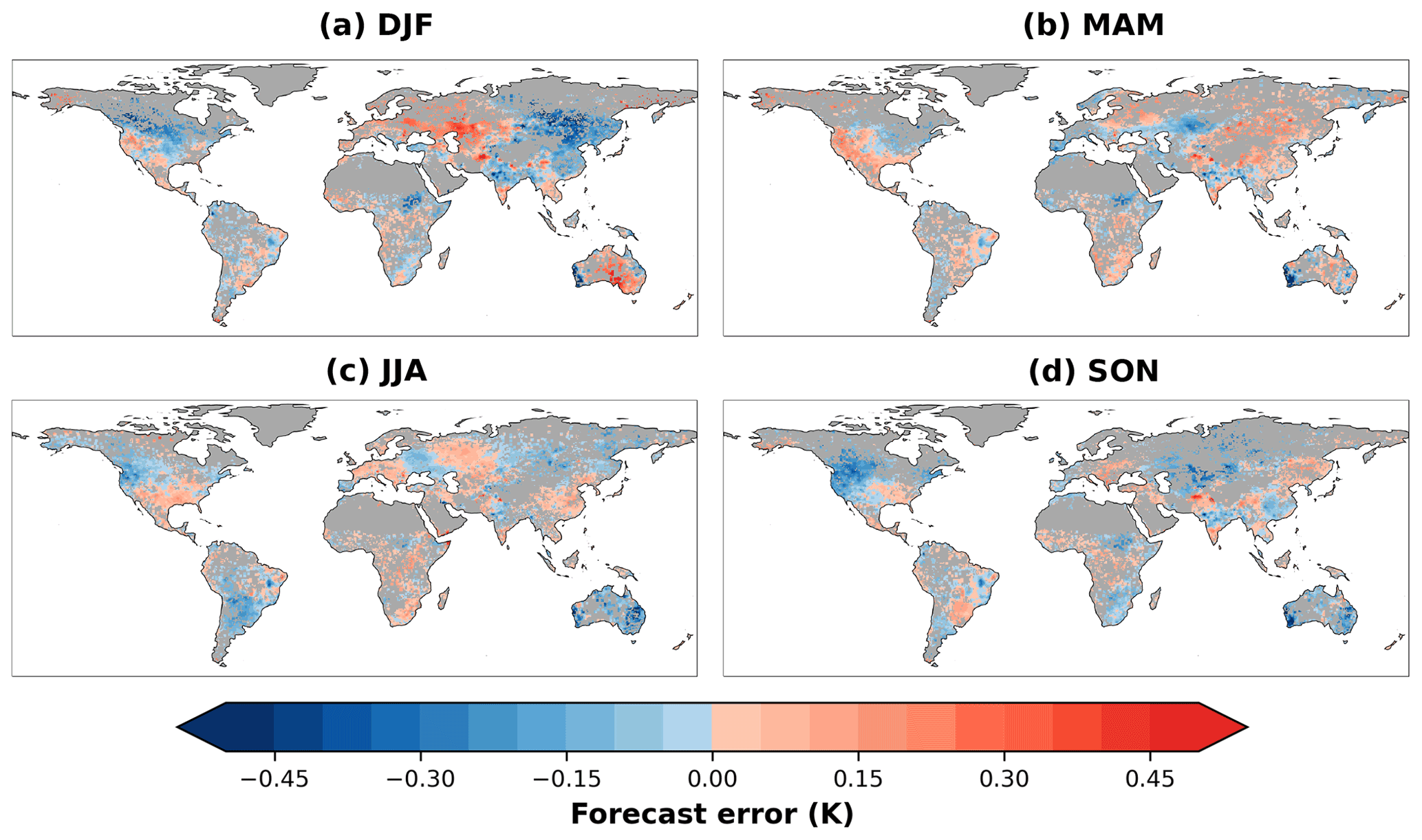
We find large errors in Asia around the Himalayas and in western North America. Dutra et al. (2021) found similar patterns in temperature forecast error patterns for the Northern Hemisphere, which they linked with the imperfect model representations of snow and soil freezing. In the tropics, the biases are smaller than in the extratropics, probably because the predictability in tropical areas is provided mainly by slowly-varying forcings such as ENSO, while extratropic predictability is mostly derived from synoptic-scale atmospheric dynamics (Jiang et al., 2017; de Andrade et al., 2019; Judt, 2020). Moreover, forecast errors in the extratropics might be larger than in the tropics due to a higher temperature variability (Tamarin-Brodsky et al., 2020).
The largest biases occur mainly around grid cells with low observational station density (as seen in Balsamo et al., 2018), and mountainous regions, especially in DJF and MAM (Fig. A2). We attribute this to three possible reasons: (i) difficulties in representing hydrometeorological processes such as freezing and thawing in those regions (Hagedorn et al., 2008), (ii) the misrepresentation of mountain topography in the land surface model (Bento et al., 2017), and (iii) low observational station density implies greater uncertainty in the interpolation of the reference temperature dataset.
3.2 Relationships between temperature forecast errors and Earth system variables
Focusing on the Earth system variables with the strongest correlation with temperature forecast errors within a grid cell, we find that climate variables are overall most relevant at the global scale (Fig. 3). Variables in the climate group are also the most studied variables in terms of improving temperature forecast skill. For example, an inaccurate SST representation in climate models is associated with ENSO biases, which in turn affect temperature and precipitation on land (Kim et al., 2017; Ehsan et al., 2021; Liu et al., 2021). The most relevant individual variables for this group are precipitation and surface solar radiation (Table 3), which control the land–atmosphere interactions and specifically surface temperature through their influence on the water and energy balances, respectively. Since the forecasts are initialized with data from the model-based ERA5 reanalysis, errors in forcing data (e.g., precipitation) can propagate to temperature forecasts with time.
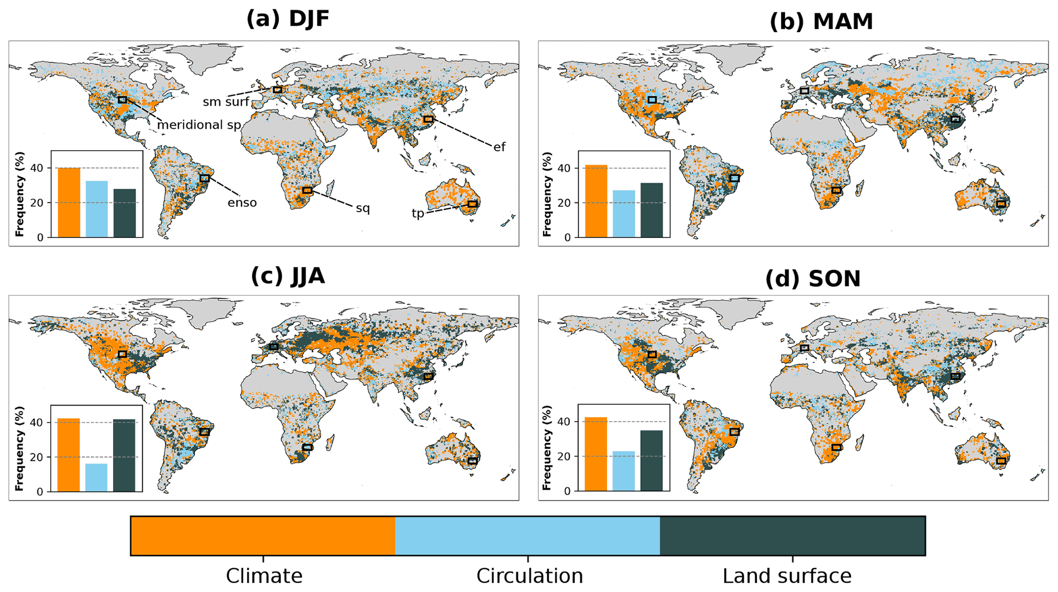
Figure 3Groups of Earth system variables to which the variable with the strongest correlation with temperature forecast error belongs (based on Fig. A3). Results shown for each season (DJF, MAM, JJA, SON). The inset bar plots show the percentage of grid cells where variables from each group are most related to temperature forecast errors. The regions outlined in black are discussed in detail in Sect. 3.3: specific humidity region (sq), evaporative fraction region (ef), total precipitation region (tp), surface soil moisture region (sm surf), meridional surface pressure differences region (meridional sp), and ENSO region (enso).
Table 3The three most important variables for each group of variables across seasons. The first number in parentheses is the absolute spatial average correlation of the variable with temperature forecast error. The second number in parenthesis is the variable's frequency of occurrence as the most relevant one.
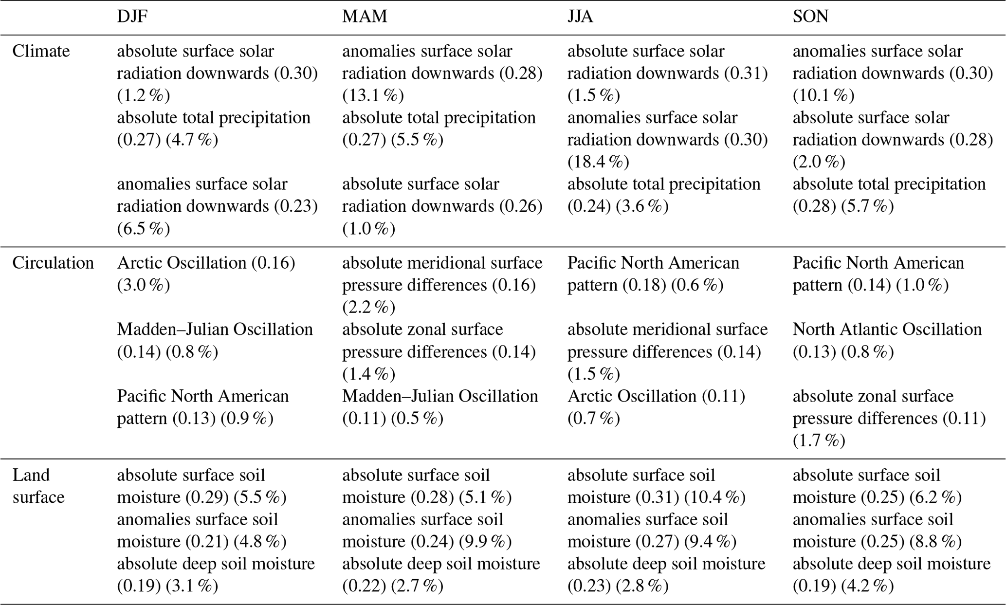
The second most relevant group is the land surface, dominated by soil moisture as the most important variable within this group. We find that the soil moisture, especially the moisture in the uppermost layer (Table 3), is important in the Northern Hemisphere during MAM and JJA (Fig. 3). Soil moisture plays a key role in the exchange of heat and water between both land and atmosphere and is one of the most studied land surface variables as a source of subseasonal predictability (Seneviratne et al., 2010; Guo et al., 2011; Orth and Seneviratne, 2014; Koster et al., 2017, 2020). Furthermore, soil moisture affects temperature forecasts particularly through its profound memory characteristics, which effectively project dry or wet anomalies into the future (Koster and Suarez, 2001; Orth and Seneviratne, 2012; Galarneau and Zeng, 2020). As a result, they can affect temperature forecast quality in regions with strong land–atmosphere coupling (Koster et al., 2004; Orth, 2021). Many recent model developments are targeted at an improved representation of soil moisture dynamics and soil moisture data assimilation, and given our results, this is a promising avenue towards reducing biases in temperature estimates (Koster et al., 2011; Albergel et al., 2013; Dirmeyer and Halder, 2017; Dirmeyer et al., 2018).
Koster et al. (2004) highlighted Africa, North America, and India as global “hotspots” of land–atmosphere coupling in JJA, therefore it is expected that soil moisture-related variables would be particularly relevant for forecast errors there. While soil moisture does not appear to be the most relevant variable (Fig. A3), the land surface variables are still largely related to temperature forecast errors in JJA across these regions. Furthermore, if soil moisture is not the most relevant driver for forecast errors in those regions during strong land–atmosphere coupling, it might be because the climate and circulation variables are comparatively less well assimilated/represented. This way, we think that other processes related with precipitation, such as cloud formation and the migration of the intertropical convergence zone (ITCZ), may be more relevant in those regions.
Along with soil moisture, vegetation plays a primary role in land–atmosphere interactions and associated heat and water exchanges. The vegetation-related variables from the land surface group (EVI and EF) are important in some regions of South America and Africa (Fig. A3). These regions were also identified in a similar study by Boussetta et al. (2015) as regions where vegetation information, in terms of LAI and albedo anomalies, had a positive impact on the temperature forecast quality. Even though the role of vegetation information on temperature forecast skill has not been as extensively addressed as that of other variables, some studies have highlighted its positive impacts in reducing forecast errors (Boussetta et al., 2013; Koster and Walker, 2015; Nogueira et al., 2020).
We find that variables from the circulation group are the least relevant for explaining temperature forecast errors globally; their importance is confined to small regions scattered across the world. The most relevant variables within this group are the large-scale circulation indices NAO and MJO and the zonal and meridional surface pressure differences (Table 3), which determine large-scale advection of air masses and hence the spatial temperature fields. A case study on this matter was presented by Grams et al. (2018). They found a connection between a strong temperature bias over Europe, predicted with the ECMWF's Integrated Forecasting System, and the misrepresentation in the onset of a blocking regime. This misrepresentation generated a chain reaction in simulated latent heat release that amplified and propagated the forecast error to a larger region. Such a finding reveals the potential of the assimilation of circulation information to reduce forecast errors and uncertainties (Lei and Anderson, 2014; Smith et al., 2020).
The overall picture of the importance of each group does not substantially change with lead time (Fig. A4). Around 18 % of the grid cells show (absolute) correlations higher than 0.3 (Fig. 4). The strongest correlations (>0.6) and hence most promising regions for improvement are found in eastern South America, eastern Europe, Southeast Asia, and southern Africa. It should, however, be noted that despite being significant after correction for multiple testing, and also being substantially different from correlations based on non-sense data (Fig. A5), these correlations from the present exploratory analysis do not directly indicate the extent to which the forecast error could potentially be improved based on these variables.
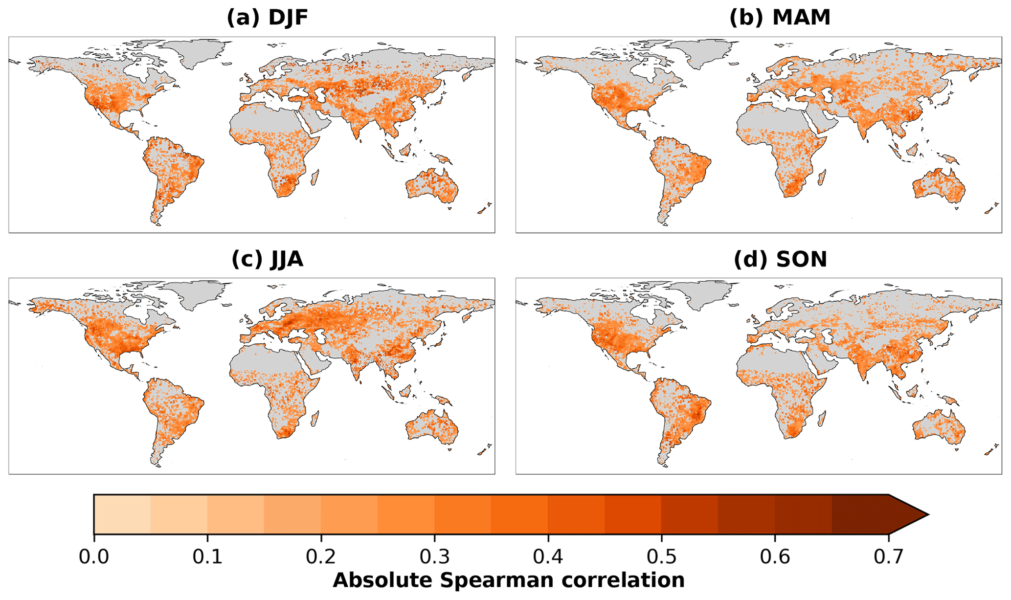
Figure 4Strongest absolute Spearman correlation coefficient between the Earth system variables in Table 1 and the temperature forecast error. The values correspond to the respective most relevant individual variables shown in Fig. A3. Only correlations that are significant after correction for multiple testing are considered.
We acknowledge that some of the selected Earth system variables, especially those that belong to the climate group, are highly correlated (Fig. A6). The most cross-correlated variables are surface terrestrial radiation downwards, sea surface temperatures, specific humidity, and snow cover fraction. Nevertheless, with our approach of individual correlations between each variable and the temperature forecast error we avoid the risk of co-linearities among the set of variables.
Next, we focus separately on the relevance of each group of variables for temperature forecast errors, as this may be hidden behind the most relevant group/variable but still exhibit significant correlations. The climate group is not only the most important group from a global perspective (Fig. 3), but it also shows significant correlations in many areas where it is not top ranked (Fig. 5). Land surface variables are globally relevant for forecast errors in similar areas as the climate group. The partly coinciding relevance of the climate and land surface groups is related to the strong coupling between them, as for example solar radiation or precipitation are related to soil moisture, vegetation state, and evapotranspiration. The circulation group is still found to be of minor relevance at the global scale. We attribute this to the short timescale variability of the circulation variables such as the winds and the surface pressure differences.
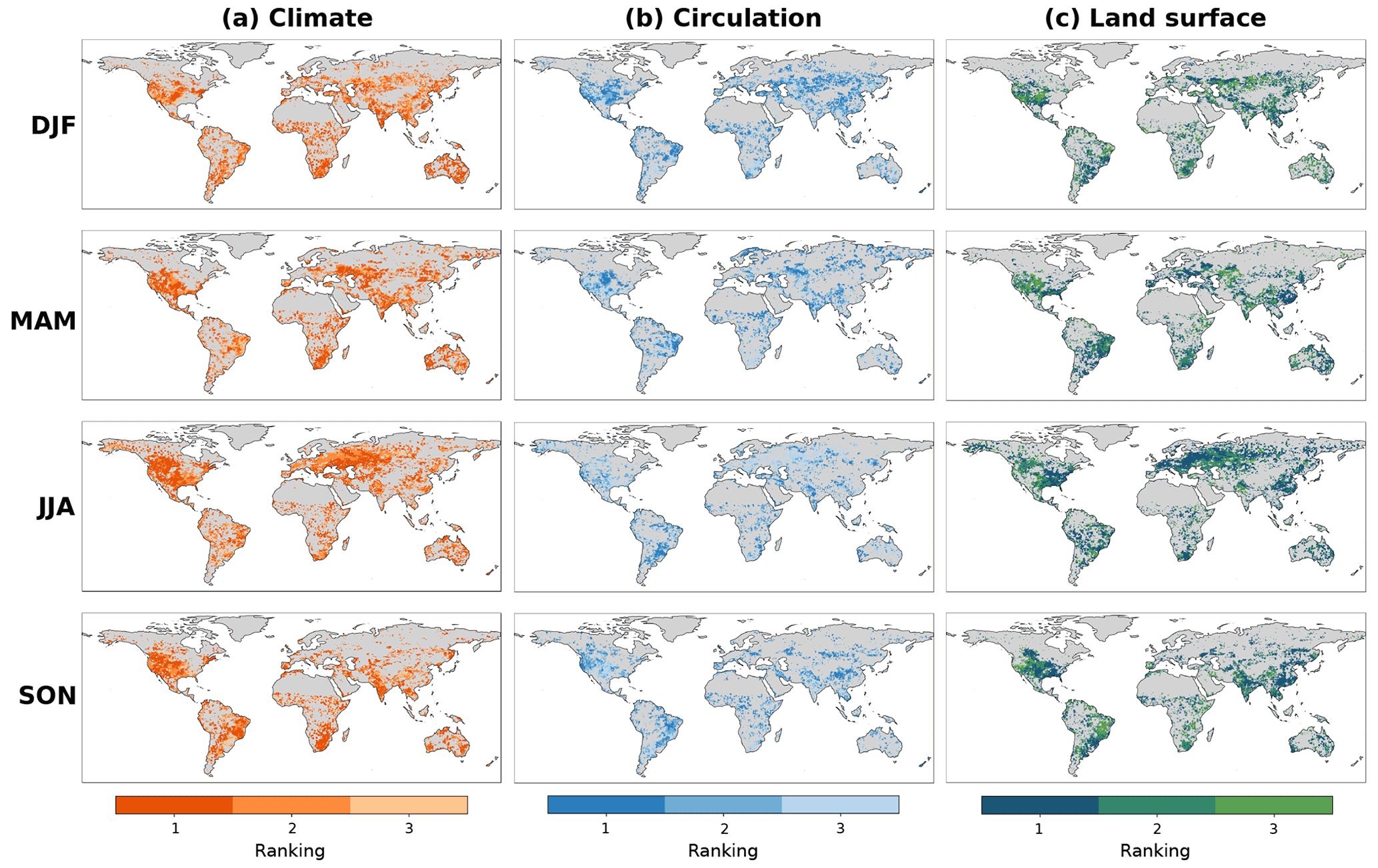
Figure 5Ranking of groups of Earth system variables (climate, circulation, and land surface) according to the Spearman correlation coefficient of the most relevant variable within each group. Gray areas indicate that no variable from the group exhibits a significant correlation with temperature forecast errors.
3.3 Possible physical mechanisms behind forecast errors in focus regions
Within the six focus regions highlighted in Fig. 3, the relationships between forecast errors and its most relevant predictors show strong seasonal variations (Fig. 6). In the sq focus region (first row in Fig. 6), the most relevant variable is specific humidity during the onset of the regional warm season (SON). We mainly find errors close to zero around zero specific humidity anomalies and increasing errors magnitude with increasing specific humidity anomalies. Incorrect initial humidity status can lead to forecast errors in temperature through multiple ways: (i) the potential for cloud formation and related reduced incoming solar radiation depends on the amount of water vapor in the air, (ii) evapotranspiration is largely determined by convergence of water vapor, and (iii) water vapor content in the air affects plant's stomatal resistance and therefore evaporative cooling. We attribute these temperature forecast errors to an inadequate representation of these three processes in the forecasting system.
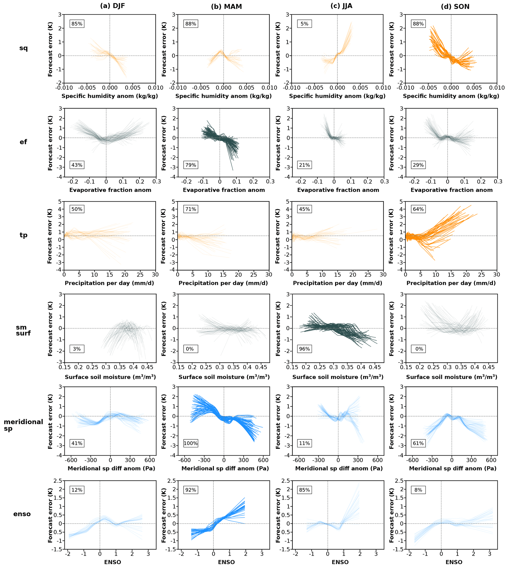
Figure 6Relationships between the most relevant Earth system variable and forecast error in the focus regions introduced in Table 2 and Fig. 3: specific humidity region (sq), evaporative fraction region (ef), total precipitation region (tp), surface soil moisture region (sm surf), meridional surface pressure differences region (meridional sp), and ENSO region (enso) (top to bottom). Relationships are shown for all seasons as smoothing lines (loess filter) fitted to the underlying point data; each line represents the relationship at one grid pixel. Light-colored smoothing lines indicate that the variable is not the most relevant in the respective season and is only shown for completeness. Inset numbers represent the percentage of grid cells in each region with significant correlation between forecast error and the Earth system variable.
The most relevant variable in the ef focus region (second row in Fig. 6) is evaporative fraction anomaly. For negative (positive) values of this variable, we see overestimation (underestimation) of temperature. One possible reason is the outdated representation of the low vegetation cover in the Hydrology Tiled ECMWF Scheme for Surface Exchanges over Land (HTESSEL) around this region, as found in Boussetta et al. (2021). An inaccurate prescription of vegetation type and cover fraction can lead to a misrepresented evapotranspiration response resulting in temperature errors.
In the tp focus region (third row in Fig. 6), the most relevant variable is precipitation. The region is semi-arid, therefore it is expected that precipitation events affect air temperature. We mainly see the influence of precipitation on temperature forecast errors after a threshold around 10 mm d−1, and generally the related errors are positive. One pathway in which precipitation influences temperature after 3 weeks lead time is through the infiltration in the soil and the subsequent evaporative cooling (Miralles et al., 2012; Orth and Seneviratne, 2014). We attribute this association between large precipitation values and positive temperature forecast errors with the misrepresentation of the evaporative cooling resulting from elevated (surface) soil moisture in this region.
In the sm surf focus region (fourth row in Fig. 6), the surface soil moisture is the most relevant variable. During JJA, there is temperature overestimation (underestimation) in the presence of low (high) soil moisture content. This region is located in a transitional climate regime (between water and energy-controlled conditions) where the land–atmosphere coupling is typically strong (Seneviratne et al., 2010; Orth, 2021). The strong variability between the smoothing lines in this region in Fig. 6 reflects the heterogeneous land surface with variable soil and vegetation characteristics. This is particularly difficult to represent in the forecasting model, and similar to sq focus region, the sm surf focus region's vegetation representation in HTESSEL is outdated, for both low and high vegetation cover (Boussetta et al., 2021), therefore we attribute the high correlation between temperature forecast errors and soil moisture to the misrepresentation of the land–atmosphere coupling.
For the meridional sp focus regions (fifth row in Fig. 6), the most relevant variable is related to processes that drive wind's magnitude and direction and also moisture and heat flux transport. The representation of winds in these regions might be affected also by the high biases in the vegetation cover in HTESSEL which include potentially erroneous assumptions on surface roughness. Even though these processes mainly occur over short timescales, there are cases in which a blocking regime can last for several days and affect temperature forecasts (Grams et al., 2018).
The ENSO focus region (sixth row in Fig. 6) is located in eastern South America. ENSO is the main source of interannual hydroclimatic variability in this region (Poveda et al., 2006; Arias et al., 2021). We see overestimation (underestimation) of temperature during the positive (negative) phase of ENSO. The positive phase is associated with reduction in precipitation and increase in surface temperature over the region. By contrast, its negative phase is associated with an increase in precipitation and a reduction in surface temperature (Wang, 2004; Salas et al., 2020). These changes also modify the strength of the regional winds (both easterlies and westerlies) that can additionally explain the temperature forecasting errors found along with increased magnitude of ENSO index values.
3.4 What is the potential to improve temperature forecasts at the S2S timescale?
We identify in Fig. 7 regions where (i) forecast errors are relatively high and (ii) rather well explained with any of the considered Earth system variables, which indicates some potential for improvement. We use the quantile criteria described in Sect. 2.5. Regions that exceed the 90th percentile in both tested conditions have the highest potential for improvement. We find the most promising regions around the Northern Hemisphere extratropics, especially in western North America, eastern Europe, and in the eastern Himalayas. We also see medium potential over some regions in central Africa, western Australia, and central and eastern South America. These regions display a climate variable as the most relevant Earth system variable. This could be due to (i) deficiencies in the assimilation of climate variables prior to forecast initialization, and (ii) imperfect process representations in the forecasting model which limits its ability to accurately propagate the initial climate state into the subsequent weeks. In the case of the climate variables, the detected potential for improving temperature forecasts is probably related to sparse precipitation observations available for assimilation, and an imperfect representation of the coupling of precipitation and radiation with temperature in the model. The latter might be more relevant in Europe and North America with transitional conditions between energy and water-controlled evapotranspiration, while additional precipitation information could probably improve forecasts around the Himalayas and in some regions in Africa.

In contrast, we find relatively low potential mainly across eastern North America, Australia, and India. This low potential is probably related to low forecast errors (Fig. 2) and not necessarily low correlation values (Fig. 4).
We analyze temperature forecast errors in subseasonal forecasts of the ECMWF and their relationship with a set of Earth system variables. Thereby we compute correlations between forecast errors and Earth system variables as a measure of their potential to inform even more accurate temperature forecasts. While previous studies have assessed the role of individual (sets of) variables, we move beyond the state of the art by analyzing a comprehensive set of Earth system variables covering multiple components of this system including several potential sources of subseasonal forecast skill.
The results show that climate-related variables, particularly precipitation and surface solar radiation, are globally the most relevant variables from our considered set of Earth system variables. There is still room for improvement in terms of climate data assimilation in data-sparse regions, and in terms of the modeled evolution of the climate over the forecasting period through, for instance, continuously improving descriptions of e.g., atmospheric dynamics, convection, and condensation schemes.
Next to this, the land surface-related variables, particularly surface soil moisture, are also important in many regions. This is specially relevant for subseasonal forecasts given the profound memory characteristics of land surface variables for which anomalies present at the forecast start can persist for weeks or months. Although to a smaller extent than for the climate predictors, we find regions and seasons in which the land surface information is strongly correlated with the temperature forecast errors. This also emphasizes the importance of accounting for the land surface variability in the weather forecasting system, thereby taking advantage of the recent developments in respective in situ observations and satellite-based data (Balsamo et al., 2018; Eyre et al., 2022). For instance, regions with water-limited conditions (typically semi-arid regions) can experience impacts of soil moisture variability on temperature (Ford et al., 2018; Jach et al., 2022). Even though surface soil moisture has less memory than deep soil moisture, we find that the first one is typically more relevant than the second one for forecast errors. This is mainly related to its more direct impact on surface temperature. Surface soil moisture affects evaporation from soils, the transpiration from short vegetation without deep-reaching roots, and the transpiration of vegetation with both shallow and deep roots as it might extract water from surface layers as long as possible. Through these pathways, it can have a significant impact on the surface energy balance and hence temperature. Furthermore, surface soil moisture typically exhibits a larger variability compared with deeper soil moisture which can also lead to stronger impacts on temperature. In dense forest regions, we expect that the deep soil moisture has a more substantial effect on temperature forecast errors than the surface soil moisture because their rooting systems are more suitable for extracting water from the deepest layers.
Moreover, the vegetation (in terms of biomass, greenness, and photosynthetic activity) can amplify the land surface effect on temperature through evaporative cooling via the LAI and stomatal resistance. This is particularly relevant at the S2S scale after extreme events like droughts and heatwaves (Bastos et al., 2020; Byrne, 2021) in regions with strong land–atmosphere coupling where vegetation functioning can be affected even after the event is over because of legacy effects such as hydraulic damage or depleted carbon reserves.
The circulation-related variables, even though they are globally the least relevant variables, also highlight regions where temperature responds to large-scale circulation patterns and surface pressure regimes. These results align with recent literature on subseasonal forecasts which contains a relatively strong focus on weather phenomena, such as NAO, MJO, and ENSO (Scaife et al., 2016; Vitart and Robertson, 2018; Mariotti et al., 2020; Falkena et al., 2022; Smith et al., 2020; Kim et al., 2021; Liu et al., 2021; Meehl et al., 2021). These phenomena are mainly driven by surface pressure differences and sea surface temperatures (Ehsan et al., 2021). An improved representation of these variables therefore offers the potential to enhance forecast skill in some regions of the world.
A main limitation in our analysis approach is that the considered Earth system variables are somewhat correlated with each other. As our methodology is based on individual correlations, it is not directly affected by relationships among the considered variables which would be the case for e.g., multivariate approaches. Yet, we note that our results can only indicate first-order effects by pinpointing the most relevant variables, and future work should focus on disentangling the joint effects of multiple variables to advance the understanding of temperature forecast errors even further. We note that the reported correlations, and the rankings between them, are not solely related to physical linkages and respective deficiencies in the forecast model and data assimilation system, but can also be affected by different levels of precision of the observational data sources. This means that noisy observation-based records might not correlate as strongly with temperature forecast errors as they would if they were measured more accurately. Therefore, our analysis reflects the current potential of each Earth system variable to inform more accurate temperature forecasts, rather than the full potential which might be exploited by even more accurate future Earth observations. Finally, our results are limited also by our considered set of Earth system variables; even though we use a comprehensive set of variables, there might be variables or states which are not yet observed at large spatial scales but relevant for improving the forecast model and its forecasts.
Despite the limitations of this study, our findings do provide information on processes that can be improved to increase the temperature forecast skill of the ECMWF–S2S forecasting system. Even though our results are based on just one forecasting system, we suggest that other forecasting models can exhibit similar patterns in sources of predictability when using the same drivers that we explore here. Machine-learning-based studies in temperature forecasts from different models at the subseasonal scale have highlighted some of the same drivers found here as important sources of predictability (Herman and Schumacher, 2018; Rasp et al., 2020; Ardilouze et al., 2021). Accurate predictions at this timescale are particularly important for issuing early warnings of extreme events, for adequately managing resources, and, more importantly, for minimizing human risks (White et al., 2017; Vitart and Robertson, 2018).

Figure A1Sum of the temperature stations located in each grid cell and its eight neighboring grid cells. This map is used to mask out regions with no temperature observations. Data available at ftp://ftp.cpc.ncep.noaa.gov/cadb_v2/library/ (last access: 23 January 2022).

Figure A2Heat maps of forecast error according to the number of CPC stations around the grid cells (x axis) and the quartiles of standard deviation of altitude in the grid cells (y axis).
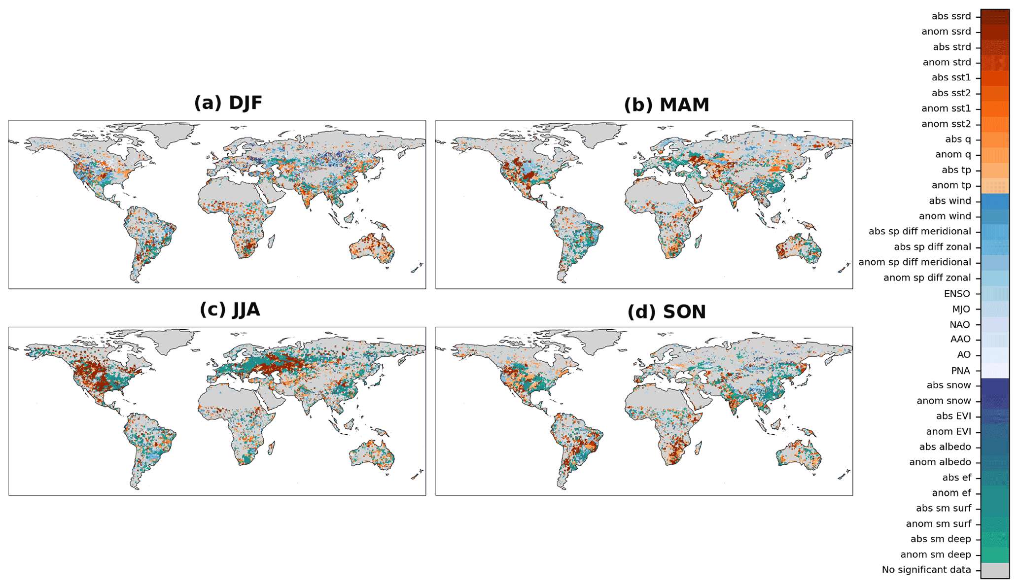
Figure A3Seasonal cycle of each grid cell's most relevant Earth system variable in terms of its relationship with forecast error. The three groups of colors represent the three groups of Earth system variables: climate (orange), circulation (light blue), and land surface (viridis). Grid cells with no significant Spearman correlation are colored in gray. A NetCDF file with these data is provided in the Supplement.
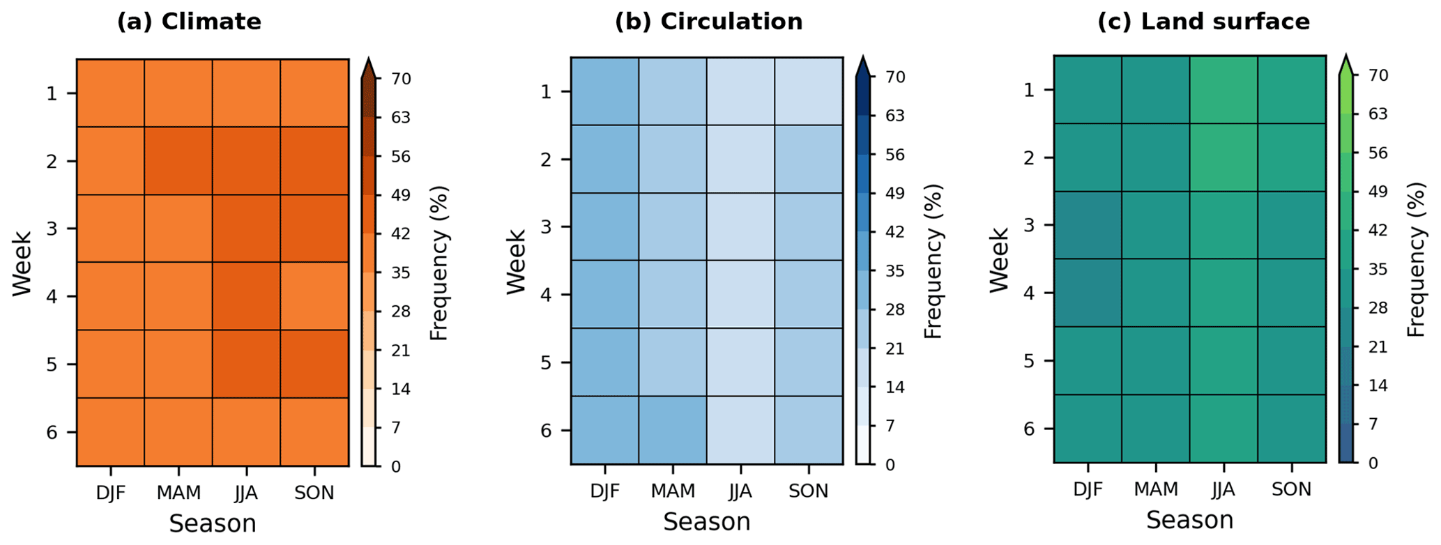
Figure A4Fraction of grid cells (%) where each group of Earth system variables is the most relevant across lead times (y axis) for each season (x axis).
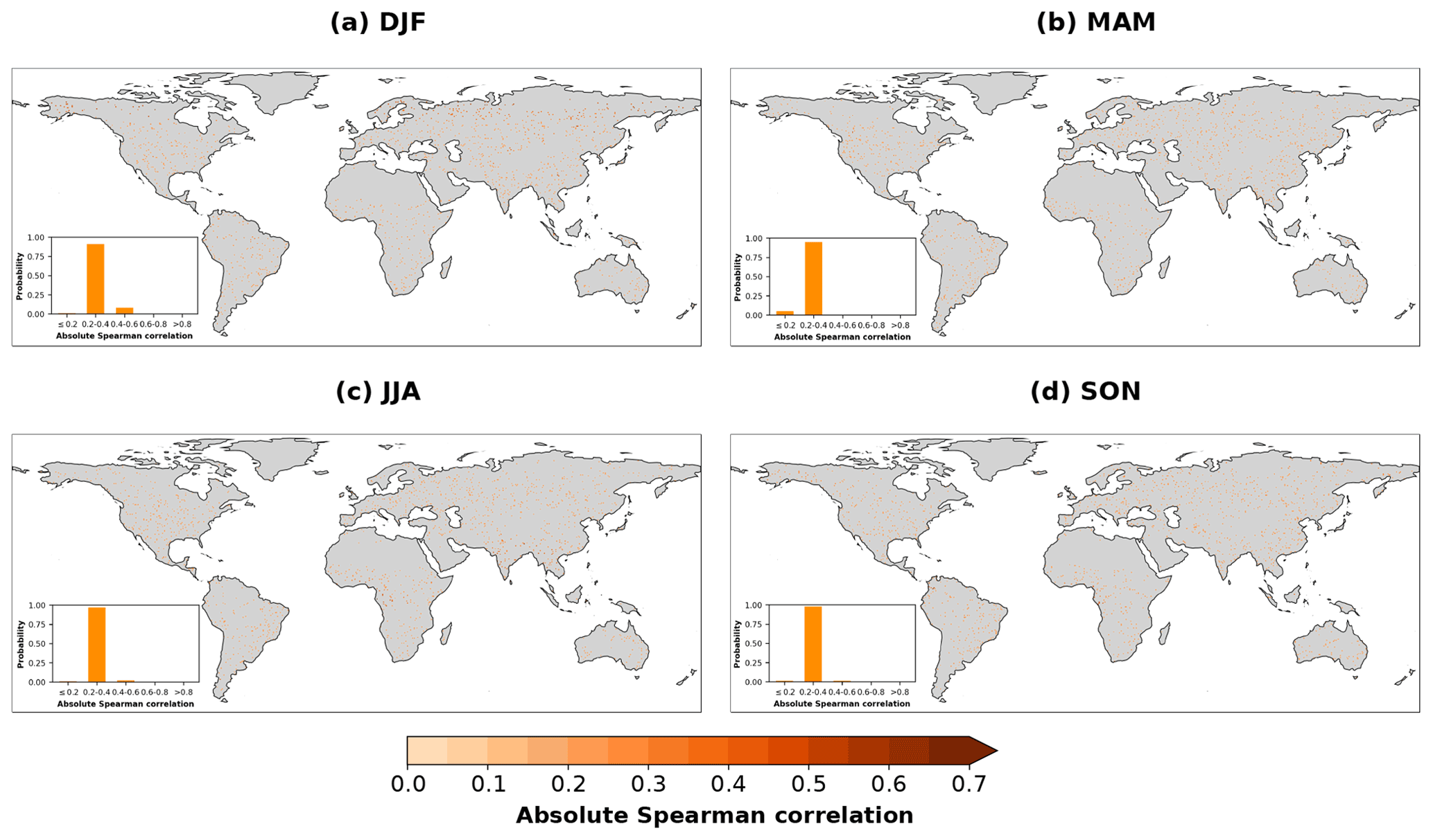
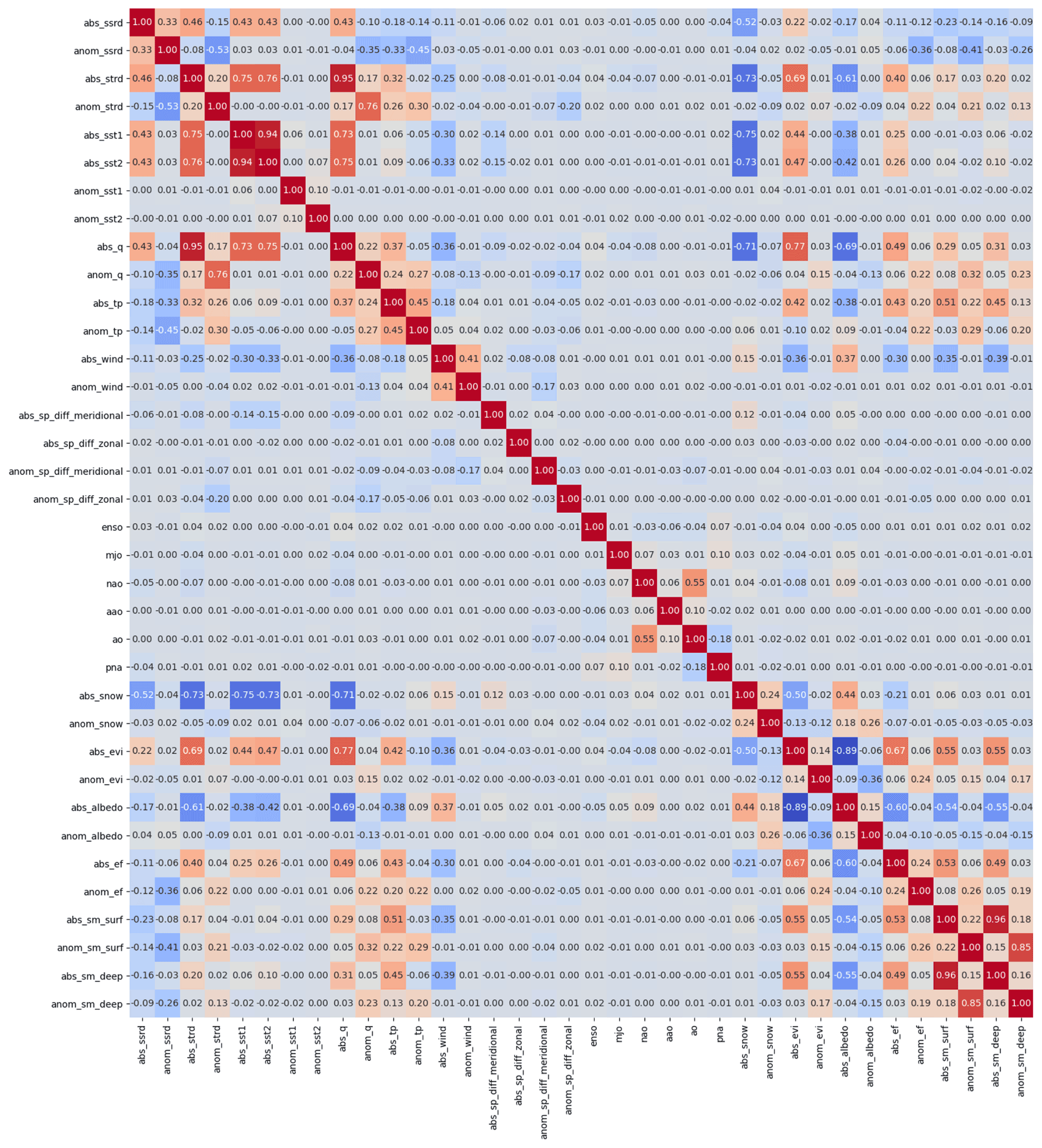
Figure A6Spearman cross-correlation matrix among the 36 considered Earth system variables. A PDF version of this plot is provided in the Supplement.
The S2S forecast temperature data are available at https://apps.ecmwf.int/datasets/data/s2s/ (ECMWF, 2013). The CPC reference temperature data are available at https://psl.noaa.gov/data/gridded/data.cpc.globaltemp.html (NOAA PSL, 2021). The variables from ERA5 are available at https://cds.climate.copernicus.eu/ (ECMWF, 2018). The precipitation data from GPCP are available at https://www.ncei.noaa.gov/products/climate-data-records/precipitation-gpcp-daily (NOAA National Centers for Environmental Information, 2017). The El Niño 3.4 index is available at https://climexp.knmi.nl/selectdailyindex.cgi?id=someone@somewhere (WMO, 2021). The MJO data are available at http://www.bom.gov.au/climate/mjo/ (Australian Government Bureau of Meteorology, 2021). The NAO, PNA, AAO, and AO circulation indices data from NOAA are available at ftp://ftp.cpc.ncep.noaa.gov/cwlinks/ (Climate Prediction Center, NOAA National Centers for Environmental Information, 2022). The EVI and albedo data from MODIS are available through NASA's data catalogue at https://lpdaac.usgs.gov/products/mod13c1v006/ (NASA EOSDIS Land Processes DAAC, 2015a) and https://lpdaac.usgs.gov/products/mcd43d42v006/ (NASA EOSDIS Land Processes DAAC, 2015b), respectively. The snow data from MODIS are available through the National Snow & Ice Data Center catalogue at https://nsidc.org/data/MOD10A1/versions/61/ (NASA National Snow and Ice Data Center Distributed Active Archive Center, 2021a). Both the evaporative fraction data from FLUXCOM and the soil moisture data from SoMo.ml are available at the Data Portal of the Max Planck Institute for Biogeochemistry at https://www.bgc-jena.mpg.de/geodb/projects/Data.php (Max Planck Institute for Biogeochemistry, 2019, 2021).
The supplement related to this article is available online at: https://doi.org/10.5194/esd-13-1451-2022-supplement.
MRV, SO, AlB, and RO jointly designed the study. MRV performed the computations and data analysis. UW carried out data acquisition and formatting. MRV, SO, AlB, RDK, GB, GA, AnB, MR, and RO contributed to the writing of the paper and the discussion and interpretation of the results.
The contact author has declared that none of the authors has any competing interests.
Publisher's note: Copernicus Publications remains neutral with regard to jurisdictional claims in published maps and institutional affiliations.
We thank Frederic Vitart for his guidance with the S2S data acquisition and the Hydrosphere–Biosphere–Climate Interactions group in the Biogeochemical Integration Department of the Max Planck Institute for Biogeochemistry for fruitful discussions that have contributed to the interpretation of the results and the design of the figures.
Melissa Ruiz-Vásquez was supported by the International Max Planck Research School for Global Biogeochemical Cycles (IMPRS). René Orth was supported by the German Research Foundation (Emmy Noether grant no. 391059971). Sungmin O received funding from the Brain Pool program, funded by the Ministry of Science and ICT through the National Research Foundation of Korea (grant no. NRF-2021H1D3A2A02040136).
The article processing charges for this open-access publication were covered by the Max Planck Society.
This paper was edited by Olivia Martius and reviewed by two anonymous referees.
Albergel, C., Dorigo, W., Reichle, R. H., Balsamo, G., de Rosnay, P., Muñoz-Sabater, J., Isaksen, L., de Jeu, R., and Wagner, W.: Skill and Global Trend Analysis of Soil Moisture from Reanalyses and Microwave Remote Sensing, J. Hydrometeorol., 14, 1259–1277, https://doi.org/10.1175/JHM-D-12-0161.1, 2013. a
Albergel, C., Dutra, E., Bonan, B., Zheng, Y., Munier, S., Balsamo, G., de Rosnay, P., Muñoz-Sabater, J., and Calvet, J.-C.: Monitoring and Forecasting the Impact of the 2018 Summer Heatwave on Vegetation, Remote Sens.-Basel, 11, 520, https://doi.org/10.3390/rs11050520, 2019. a
Ardilouze, C., Specq, D., Batté, L., and Cassou, C.: Flow dependence of wintertime subseasonal prediction skill over Europe, Weather Clim. Dynam., 2, 1033–1049, https://doi.org/10.5194/wcd-2-1033-2021, 2021. a
Arias, P. A., Garreaud, R., Poveda, G., Espinoza, J. C., Molina-Carpio, J., Masiokas, M., Viale, M., Scaff, L., and van Oevelen, P. J.: Hydroclimate of the Andes Part II: Hydroclimate Variability and Sub–Continental Patterns, Front. Earth Sci., 8, 505467, https://doi.org/10.3389/feart.2020.505467, 2021. a
Australian Government Bureau of Meteorology: Madden-Julian Oscillation (MJO), Australian Government Bureau of Meteorology [data set], http://www.bom.gov.au/climate/mjo/, last access: 11 August 2021. a
Balsamo, G., Agusti-Panareda, A., Albergel, C., Arduini, G., Beljaars, A., Bidlot, J., Blyth, E., Bousserez, N., Boussetta, S., Brown, A., Buizza, R., Buontempo, C., Chevallier, F., Choulga, M., Cloke, H., Cronin, M. F., Dahoui, M., De Rosnay, P., Dirmeyer, P. A., Drusch, M., Dutra, E., Ek, M. B., Gentine, P., Hewitt, H., Keeley, S. P., Kerr, Y., Kumar, S., Lupu, C., Mahfouf, J.-F., McNorton, J., Mecklenburg, S., Mogensen, K., Muñoz-Sabater, J., Orth, R., Rabier, F., Reichle, R., Ruston, B., Pappenberger, F., Sandu, I., Seneviratne, S. I., Tietsche, S., Trigo, I. F., Uijlenhoet, R., Wedi, N., Woolway, R. I., and Zeng, X.: Satellite and In Situ Observations for Advancing Global Earth Surface Modelling: A Review, Remote Sens.-Basel, 10, 2038, https://doi.org/10.3390/rs10122038, 2018. a, b, c
Barber, C. B., Dobkin, D. P., and Huhdanpaa, H.: The Quickhull Algorithm for Convex Hulls, ACM T. Math. Software, 22, 469–483, https://doi.org/10.1145/235815.235821, 1996. a
Bastos, A., Ciais, P., Friedlingstein, P., Sitch, S., Pongratz, J., Fan, L., Wigneron, J. P., Weber, U., Reichstein, M., Fu, Z., Anthoni, P., Arneth, A., Haverd, V., Jain, A. K., Joetzjer, E., Knauer, J., Lienert, S., Loughran, T., McGuire, P. C., Tian, H., Viovy, N., and Zaehle, S.: Direct and seasonal legacy effects of the 2018 heat wave and drought on European ecosystem productivity, Science Advances, 6, eaba2724, https://doi.org/10.1126/sciadv.aba2724, 2020. a
Bauer, P., Thorpe, A., and Brunet, G.: The quiet revolution of numerical weather prediction, Nature, 525, 47–55, https://doi.org/10.1038/nature14956, 2015. a
Benjamini, Y. and Hochberg, Y.: Controlling the False Discovery Rate: A Practical and Powerful Approach to Multiple Testing, J. Roy. Stat. Soc. B Met., 57, 289–300, https://doi.org/10.2307/2346101, 1995. a
Bento, V. A., DaCamara, C. C., Trigo, I. F., Martins, J. P. A., and Duguay-Tetzlaff, A.: Improving Land Surface Temperature Retrievals over Mountainous Regions, Remote Sens.-Basel, 9, 38, https://doi.org/10.3390/rs9010038, 2017. a
Boussetta, S., Balsamo, G., Beljaars, A., Kral, T., and Jarlan, L.: Impact of a satellite-derived leaf area index monthly climatology in a global numerical weather prediction model, Int. J. Remote Sens., 34, 3520–3542, https://doi.org/10.1080/01431161.2012.716543, 2013. a, b
Boussetta, S., Balsamo, G., Dutra, E., Beljaars, A., and Albergel, C.: Assimilation of surface albedo and vegetation states from satellite observations and their impact on numerical weather prediction, Remote Sens. Environ., 163, 111–126, https://doi.org/10.1016/j.rse.2015.03.009, 2015. a, b
Boussetta, S., Balsamo, G., Arduini, G., Dutra, E., McNorton, J., Choulga, M., Agustí-Panareda, A., Beljaars, A., Wedi, N., Munõz-Sabater, J., de Rosnay, P., Sandu, I., Hadade, I., Carver, G., Mazzetti, C., Prudhomme, C., Yamazaki, D., and Zsoter, E.: ECLand: The ECMWF Land Surface Modelling System, Atmosphere, 12, 723, https://doi.org/10.3390/atmos12060723, 2021. a, b
Brunet, G., Shapiro, M., Hoskins, B., Moncrieff, M., Dole, R., Kiladis, G. N., Kirtman, B., Lorenc, A., Mills, B., Morss, R., Polavarapu, S., Rogers, D., Schaake, J., and Shukla, J.: Collaboration of the Weather and Climate Communities to Advance Subseasonal-to-Seasonal Prediction, B. Am. Meteorol. Soc., 91, 1397–1406, https://doi.org/10.1175/2010BAMS3013.1, 2010. a
Büeler, D., Ferranti, L., Magnusson, L., Quinting, J. F., and Grams, C. M.: Year-round sub-seasonal forecast skill for Atlantic–European weather regimes, Q. J. Roy. Meteor. Soc., 147, 4283–4309, https://doi.org/10.1002/qj.4178, 2021. a
Byrne, M. P.: Amplified warming of extreme temperatures over tropical land, Nat. Geosci., 14, 837–841, https://doi.org/10.1038/s41561-021-00828-8, 2021. a
Climate Prediction Center (CPC), NOAA National Centers for Environmental Information: Climate & Weather linkage Teleconnections, CPC, NOAA [data set], ftp://ftp.cpc.ncep.noaa.gov/cwlinks/, last access: 30 March 2022. a
Cortés, J., Mahecha, M., Reichstein, M., and Brenning, A.: Accounting for multiple testing in the analysis of spatio-temporal environmental data, Environ. Ecol. Stat., 27, 293–318, https://doi.org/10.1007/s10651-020-00446-4, 2020. a
de Andrade, F. M., Coelho, C. A. S., and Cavalcanti, I. F. A.: Global precipitation hindcast quality assessment of the Subseasonal to Seasonal (S2S) prediction project models, Clim. Dynam., 52, 5451–5475, https://doi.org/10.1007/s00382-018-4457-z, 2019. a, b
Dirmeyer, P. A. and Halder, S.: Application of the Land–Atmosphere Coupling Paradigm to the Operational Coupled Forecast System, Version 2 (CFSv2), J. Hydrometeorol., 18, 85–108, https://doi.org/10.1175/JHM-D-16-0064.1, 2017. a, b
Dirmeyer, P. A., Halder, S., and Bombardi, R.: On the Harvest of Predictability From Land States in a Global Forecast Model, J. Geophys. Res.-Atmos., 123, 13111–13127, https://doi.org/10.1029/2018JD029103, 2018. a
Durai, V. R. and Bhradwaj, R.: Evaluation of statistical bias correction methods for numerical weather prediction model forecasts of maximum and minimum temperatures, Nat. Hazards, 73, 1229–1254, https://doi.org/10.1007/s11069-014-1136-1, 2014. a
Dutra, E., Johannsen, F., and Magnusson, L.: Late Spring and Summer Subseasonal Forecasts in the Northern Hemisphere Midlatitudes: Biases and Skill in the ECMWF Model, Mon. Weather Rev., 149, 2659–2671, https://doi.org/10.1175/MWR-D-20-0342.1, 2021. a
ECMWF: S2S, ECMWF, Realtime, Daily averaged, ECMWF [data set], https://apps.ecmwf.int/datasets/data/s2s/ (last access: 3 February 2021), 2013. a
ECMWF: ERA5 hourly data on single levels from 1959 to present, ECMWF [data set], https://cds.climate.copernicus.eu/, (last access: 9 March 2022), 2018. a
Ehsan, M. A., Tippett, M. K., Robertson, A. W., Almazroui, M., Ismail, M., Dinku, T., Acharya, N., Siebert, A., Ahmed, J. S., and Teshome, A.: Seasonal predictability of Ethiopian Kiremt rainfall and forecast skill of ECMWF's SEAS5 model, Clim. Dynam., 57, 3075–3091, https://doi.org/10.1007/s00382-021-05855-0, 2021. a, b
Eyre, J. R., Bell, W., Cotton, J., English, S. J., Forsythe, M., Healy, S. B., and Pavelin, E. G.: Assimilation of satellite data in numerical weather prediction. Part II: Recent years, Q. J. Roy. Meteor. Soc., 148, 521–556, https://doi.org/10.1002/qj.4228, 2022. a
Falkena, S. K., de Wiljes, J., Weisheimer, A., and Shepherd, T. G.: Detection of interannual ensemble forecast signals over the North Atlantic and Europe using atmospheric circulation regimes, Q. J. Roy. Meteor. Soc., 148, 434–453, https://doi.org/10.1002/qj.4213, 2022. a, b
Farcomeni, A.: A review of modern multiple hypothesis testing, with particular attention to the false discovery proportion, Stat. Methods Med. Res., 17, 347–388, https://doi.org/10.1177/0962280206079046, 2008. a
Ford, T. W., Dirmeyer, P. A., and Benson, D. O.: Evaluation of heat wave forecasts seamlessly across subseasonal timescales, npj Climate and Atmospheric Science, 1, 20, https://doi.org/10.1038/s41612-018-0027-7, 2018. a
Galarneau, T. J. and Zeng, X.: The Hurricane Harvey (2017) Texas Rainstorm: Synoptic Analysis and Sensitivity to Soil Moisture, Mon. Weather Rev., 148, 2479–2502, https://doi.org/10.1175/MWR-D-19-0308.1, 2020. a
Grams, C. M., Magnusson, L., and Madonna, E.: An atmospheric dynamics perspective on the amplification and propagation of forecast error in numerical weather prediction models: A case study, Q. J. Roy. Meteor. Soc., 144, 2577–2591, https://doi.org/10.1002/qj.3353, 2018. a, b
Guo, Z., Dirmeyer, P. A., and DelSole, T.: Land surface impacts on subseasonal and seasonal predictability, Geophys. Res. Lett., 38, L24812, https://doi.org/10.1029/2011GL049945, 2011. a
Hagedorn, R., Hamill, T. M., and Whitaker, J. S.: Probabilistic Forecast Calibration Using ECMWF and GFS Ensemble Reforecasts. Part I: Two-Meter Temperatures, Mon. Weather Rev., 136, 2608–2619, https://doi.org/10.1175/2007MWR2410.1, 2008. a
Herman, G. R. and Schumacher, R. S.: Money Doesn't Grow on Trees, but Forecasts Do: Forecasting Extreme Precipitation with Random Forests, Mon. Weather Rev., 146, 1571–1600, https://doi.org/10.1175/MWR-D-17-0250.1, 2018. a
Hersbach, H., Bell, B., Berrisford, P., Hirahara, S., Horányi, A., Muñoz-Sabater, J., Nicolas, J., Peubey, C., Radu, R., Schepers, D., Simmons, A., Soci, C., Abdalla, S., Abellan, X., Balsamo, G., Bechtold, P., Biavati, G., Bidlot, J., Bonavita, M., De Chiara, G., Dahlgren, P., Dee, D., Diamantakis, M., Dragani, R., Flemming, J., Forbes, R., Fuentes, M., Geer, A., Haimberger, L., Healy, S., Hogan, R. J., Hólm, E., Janisková, M., Keeley, S., Laloyaux, P., Lopez, P., Lupu, C., Radnoti, G., de Rosnay, P., Rozum, I., Vamborg, F., Villaume, S., and Thépaut, J.-N.: The ERA5 global reanalysis, Q. J. Roy. Meteor. Soc., 146, 1999–2049, https://doi.org/10.1002/qj.3803, 2020. a
Higgins, R. W., Leetmaa, A., Xue, Y., and Barnston, A.: Dominant Factors Influencing the Seasonal Predictability of U.S. Precipitation and Surface Air Temperature, J. Climate, 13, 3994–4017, https://doi.org/10.1175/1520-0442(2000)013<3994:DFITSP>2.0.CO;2, 2000.
Jach, L., Schwitalla, T., Branch, O., Warrach-Sagi, K., and Wulfmeyer, V.: Sensitivity of land–atmosphere coupling strength to changing atmospheric temperature and moisture over Europe, Earth Syst. Dynam., 13, 109–132, https://doi.org/10.5194/esd-13-109-2022, 2022. a
Jiang, M., Felzer, B. S., Nielsen, U. N., and Medlyn, B. E.: Biome-specific climatic space defined by temperature and precipitation predictability, Global Ecol. Biogeogr., 26, 1270–1282, https://doi.org/10.1111/geb.12635, 2017. a
Judt, F.: Atmospheric Predictability of the Tropics, Middle Latitudes, and Polar Regions Explored through Global Storm-Resolving Simulations, J. Atmos. Sci., 77, 257–276, https://doi.org/10.1175/JAS-D-19-0116.1, 2020. a
Jung, M., Koirala, S., Weber, U., Ichii, K., Gans, F., Camps-Valls, G., Papale, D., Schwalm, C., Tramontana, G., and Reichstein, M.: The FLUXCOM ensemble of global land-atmosphere energy fluxes, Scientific Data, 6, 74, https://doi.org/10.1038/s41597-019-0076-8, 2019. a
Kim, H., Ham, Y. G., Joo, Y. S., and Son, S. W.: Deep learning for bias correction of MJO prediction, Nat. Commun., 12, 3087, https://doi.org/10.1038/s41467-021-23406-3, 2021. a, b
Kim, S. T., Jeong, H.-I., and Jin, F.-F.: Mean bias in seasonal forecast model and ENSO prediction error, Sci. Rep.-UK, 7, 6029, https://doi.org/10.1038/s41598-017-05221-3, 2017. a
Kirtman, B. P., Min, D., Infanti, J. M., Kinter, J. L., Paolino, D. A., Zhang, Q., van den Dool, H., Saha, S., Mendez, M. P., Becker, E., Peng, P., Tripp, P., Huang, J., DeWitt, D. G., Tippett, M. K., Barnston, A. G., Li, S., Rosati, A., Schubert, S. D., Rienecker, M., Suarez, M., Li, Z. E., Marshak, J., Lim, Y.-K., Tribbia, J., Pegion, K., Merryfield, W. J., Denis, B., and Wood, E. F.: The North American Multimodel Ensemble: Phase-1 Seasonal-to-Interannual Prediction; Phase-2 toward Developing Intraseasonal Prediction, B. Am. Meteorol. Soc., 95, 585–601, https://doi.org/10.1175/BAMS-D-12-00050.1, 2014. a
Koster, R. D. and Suarez, M. J.: Soil Moisture Memory in Climate Models, J. Hydrometeorol., 2, 558–570, https://doi.org/10.1175/1525-7541(2001)002<0558:SMMICM>2.0.CO;2, 2001. a
Koster, R. D. and Walker, G. K.: Interactive Vegetation Phenology, Soil Moisture, and Monthly Temperature Forecasts, J. Hydrometeorol., 16, 1456–1465, https://doi.org/10.1175/JHM-D-14-0205.1, 2015. a, b
Koster, R. D., Dirmeyer, P. A., Guo, Z., Bonan, G., Chan, E., Cox, P., Gordon, C. T., Kanae, S., Kowalczyk, E., Lawrence, D., Liu, P., Lu, C.-H., Malyshev, S., McAvaney, B., Mitchell, K., Mocko, D., Oki, T., Oleson, K., Pitman, A., Sud, Y. C., Taylor, C. M., Verseghy, D., Vasic, R., Xue, Y., and Yamada, T.: Regions of Strong Coupling Between Soil Moisture and Precipitation, Science, 305, 1138–1140, https://doi.org/10.1126/science.1100217, 2004. a, b
Koster, R. D., Mahanama, S. P. P., Livneh, B., Lettenmaier, D. P., and Reichle, R. H.: Skill in streamflow forecasts derived from large-scale estimates of soil moisture and snow, Nat. Geosci., 3, 613–616, https://doi.org/10.1038/ngeo944, 2010a. a
Koster, R. D., Mahanama, S. P. P., Yamada, T. J., Balsamo, G., Berg, A. A., Boisserie, M., Dirmeyer, P. A., Doblas-Reyes, F. J., Drewitt, G., Gordon, C. T., Guo, Z., Jeong, J.-H., Lawrence, D. M., Lee, W.-S., Li, Z., Luo, L., Malyshev, S., Merryfield, W. J., Seneviratne, S. I., Stanelle, T., van den Hurk, B. J. J. M., Vitart, F., and Wood, E. F.: Contribution of land surface initialization to subseasonal forecast skill: First results from a multi-model experiment, Geophys. Res. Lett., 37, L02402, https://doi.org/10.1029/2009GL041677, 2010b. a
Koster, R. D., Mahanama, S. P. P., Yamada, T. J., Balsamo, G., Berg, A. A., Boisserie, M., Dirmeyer, P. A., Doblas-Reyes, F. J., Drewitt, G., Gordon, C. T., Guo, Z., Jeong, J.-H., Lee, W.-S., Li, Z., Luo, L., Malyshev, S., Merryfield, W. J., Seneviratne, S. I., Stanelle, T., van den Hurk, B. J. J. M., Vitart, F., and Wood, E. F.: The Second Phase of the Global Land–Atmosphere Coupling Experiment: Soil Moisture Contributions to Subseasonal Forecast Skill, J. Hydrometeorol., 12, 805–822, https://doi.org/10.1175/2011JHM1365.1, 2011. a
Koster, R. D., Betts, A. K., Dirmeyer, P. A., Bierkens, M., Bennett, K. E., Déry, S. J., Evans, J. P., Fu, R., Hernandez, F., Leung, L. R., Liang, X., Masood, M., Savenije, H., Wang, G., and Yuan, X.: Hydroclimatic variability and predictability: a survey of recent research, Hydrol. Earth Syst. Sci., 21, 3777–3798, https://doi.org/10.5194/hess-21-3777-2017, 2017. a
Koster, R. D., Schubert, S. D., DeAngelis, A. M., Molod, A. M., and Mahanama, S. P.: Using a Simple Water Balance Framework to Quantify the Impact of Soil Moisture Initialization on Subseasonal Evapotranspiration and Air Temperature Forecasts, J. Hydrometeorol., 21, 1705–1722, https://doi.org/10.1175/JHM-D-20-0007.1, 2020. a, b
Lei, L. and Anderson, J. L.: Impacts of Frequent Assimilation of Surface Pressure Observations on Atmospheric Analyses, Mon. Weather Rev., 142, 4477–4483, https://doi.org/10.1175/MWR-D-14-00097.1, 2014. a
Liu, B., Su, J., Ma, L., Tang, Y., Rong, X., Li, J., Chen, H., Liu, B., Hua, L., and Wu, R.: Seasonal prediction skills in the CAMS-CSM climate forecast system, Clim. Dynam., 57, 2953–2970, https://doi.org/10.1007/s00382-021-05848-z, 2021. a, b
Mariotti, A., Ruti, P. M., and Rixen, M.: Progress in subseasonal to seasonal prediction through a joint weather and climate community effort, npj Climate and Atmospheric Science, 1, 4, https://doi.org/10.1038/s41612-018-0014-z, 2018. a, b
Mariotti, A., Baggett, C., Barnes, E. A., Becker, E., Butler, A., Collins, D. C., Dirmeyer, P. A., Ferranti, L., Johnson, N. C., Jones, J., Kirtman, B. P., Lang, A. L., Molod, A., Newman, M., Robertson, A. W., Schubert, S., Waliser, D. E., and Albers, J.: Windows of Opportunity for Skillful Forecasts Subseasonal to Seasonal and Beyond, B. Am. Meteorol. Soc., 101, E608–E625, https://doi.org/10.1175/BAMS-D-18-0326.1, 2020. a, b
Max Planck Institute for Biogeochemistry: FLUXCOM, Max Plank Institute for Biogeochemistry [data set], https://www.bgc-jena.mpg.de/geodb/projects/Data.php (last access: 6 January 2022), 2019 a
Max Planck Institute for Biogeochemistry: SoMo.ml, Max Plank Institute for Biogeochemistry [data set], https://www.bgc-jena.mpg.de/geodb/projects/Data.php (last access: 6 January 2022), 2021. a
McDonnell, J., Lambkin, K., Fealy, R., Hennessy, D., Shalloo, L., and Brophy, C.: Verification and bias correction of ECMWF forecasts for Irish weather stations to evaluate their potential usefulness in grass growth modelling, Meteorol. Appl., 25, 292–301, https://doi.org/10.1002/met.1691, 2018. a
Meehl, G. A., Richter, J. H., Teng, H., Capotondi, A., Cobb, K., Doblas-Reyes, F., Donat, M. G., England, M. H., Fyfe, J. C., Han, W., Kim, H., Kirtman, B. P., Kushnir, Y., Lovenduski, N. S., Mann, M. E., Merryfield, W. J., Nieves, V., Pegion, K., Rosenbloom, N., Sanchez, S. C., Scaife, A. A., Smith, D., Subramanian, A. C., Sun, L., Thompson, D., Ummenhofer, C. C., and Xie, S.-P.: Initialized Earth System prediction from subseasonal to decadal timescales, Nature Reviews Earth & Environment, 2, 340–357, https://doi.org/10.1038/s43017-021-00155-x, 2021. a, b
Meng, X. H., Evans, J. P., and McCabe, M. F.: The Impact of Observed Vegetation Changes on Land–Atmosphere Feedbacks During Drought, J. Hydrometeorol., 15, 759–776, https://doi.org/10.1175/JHM-D-13-0130.1, 2014. a
Miller, D. E., Wang, Z., Li, B., Harnos, D. S., and Ford, T.: Skillful Subseasonal Prediction of U. S. Extreme Warm Days and Standardized Precipitation Index in Boreal Summer, J. Climate, 34, 5887–5898, https://doi.org/10.1175/JCLI-D-20-0878.1, 2021. a
Miralles, D. G., van den Berg, M. J., Teuling, A. J., and de Jeu, R. A. M.: Soil moisture-temperature coupling: A multiscale observational analysis, Geophys. Res. Lett., 39, L21707, https://doi.org/10.1029/2012GL053703, 2012. a, b, c
Miralles, D. G., Gentine, P., Seneviratne, S. I., and Teuling, A. J.: Land-atmospheric feedbacks during droughts and heatwaves: state of the science and current challenges, Ann. NY Acad. Sci., 1436, 19–35, https://doi.org/10.1111/nyas.13912, 2019. a
Mo, K. C.: Relationships between Low-Frequency Variability in the Southern Hemisphere and Sea Surface Temperature Anomalies, J. Climate, 13, 3599–3610, https://doi.org/10.1175/1520-0442(2000)013<3599:RBLFVI>2.0.CO;2, 2000. a
NASA EOSDIS Land Processes DAAC: MOD13C1 MODIS/Terra Vegetation Indices 16-Day L3 Global 0.05Deg CMG V006, NASA [data set], https://lpdaac.usgs.gov/products/mod13c1v006/ (last access: 28 April 2020), 2015a. a, b
NASA EOSDIS Land Processes DAAC: MCD43D42 MODIS/Terra+Aqua BRDF/Albedo Black Sky Albedo Band1 Daily L3 Global 30ArcSec CMG V006, NASA [data set], https://lpdaac.usgs.gov/products/mcd43d42v006/ (last access: 9 December 2021), 2015b. a
NASA EOSDIS Land Processes DAAC: MCD12C1 MODIS/Terra+Aqua Land Cover Type Yearly L3 Global 0.05Deg CMG V006, NASA [data set], https://doi.org/10.5067/MODIS/MOD13Q1.006 2015c. a
NASA National Snow and Ice Data Center Distributed Active Archive Center: MODIS/Terra Snow Cover Daily L3 Global 500m SIN Grid, Version 61, NASA [data set], https://nsidc.org/data/MOD10A1/versions/61/, last access: 11 November 2021a. a
Newman, M., Sardeshmukh, P. D., Winkler, C. R., and Whitaker, J. S.: A Study of Subseasonal Predictability, Mon. Weather Rev., 131, 1715–1732, https://doi.org/10.1175//2558.1, 2003. a
NOAA National Centers for Environmental Information: Global Precipitation Climatology Project (GPCP) Climate Data Record (CDR), Version 1.3 (Daily), NOAA [data set], https://www.ncei.noaa.gov/products/climate-data-records/precipitation-gpcp-daily (last access: 20 December 2021), 2017. a, b
NOAA PSL: CPC Global Unified Temperature, NOAA [data set], https://psl.noaa.gov/data/gridded/data.cpc.globaltemp.html, last access: 21 December 2021. a
Nogueira, M., Albergel, C., Boussetta, S., Johannsen, F., Trigo, I. F., Ermida, S. L., Martins, J. P. A., and Dutra, E.: Role of vegetation in representing land surface temperature in the CHTESSEL (CY45R1) and SURFEX-ISBA (v8.1) land surface models: a case study over Iberia, Geosci. Model Dev., 13, 3975–3993, https://doi.org/10.5194/gmd-13-3975-2020, 2020. a, b
O, S. and Orth, R.: Global soil moisture data derived through machine learning trained with in-situ measurements, Scientific Data, 8, 170, https://doi.org/10.1038/s41597-021-00964-1, 2021. a
Orth, R.: When the Land Surface Shifts Gears, AGU Advances, 2, e2021AV000414, https://doi.org/10.1029/2021AV000414, 2021. a, b
Orth, R. and Seneviratne, S. I.: Analysis of soil moisture memory from observations in Europe, J. Geophys. Res.-Atmos., 117, D15115, https://doi.org/10.1029/2011JD017366, 2012. a, b
Orth, R. and Seneviratne, S. I.: Using soil moisture forecasts for sub-seasonal summer temperature predictions in Europe, Clim. Dynam., 43, 3403–3418, https://doi.org/10.1007/s00382-014-2112-x, 2014. a, b, c
Pegion, K., Kirtman, B. P., Becker, E., Collins, D. C., LaJoie, E., Burgman, R., Bell, R., DelSole, T., Min, D., Zhu, Y., Li, W., Sinsky, E., Guan, H., Gottschalck, J., Metzger, E. J., Barton, N. P., Achuthavarier, D., Marshak, J., Koster, R. D., Lin, H., Gagnon, N., Bell, M., Tippett, M. K., Robertson, A. W., Sun, S., Benjamin, S. G., Green, B. W., Bleck, R., and Kim, H.: The Subseasonal Experiment (SubX): A Multimodel Subseasonal Prediction Experiment, B. Am. Meteorol. Soc., 100, 2043–2060, https://doi.org/10.1175/BAMS-D-18-0270.1, 2019. a, b
Pendergrass, A. G., Meehl, G. A., Pulwarty, R., Hobbins, M., Hoell, A., AghaKouchak, A., Bonfils, C. J. W., Gallant, A. J. E., Hoerling, M., Hoffmann, D., Kaatz, L., Lehner, F., Llewellyn, D., Mote, P., Neale, R. B., Overpeck, J. T., Sheffield, A., Stahl, K., Svoboda, M., Wheeler, M. C., Wood, A. W., and Woodhouse, C. A.: Flash droughts present a new challenge for subseasonal-to-seasonal prediction, Nat. Clim. Change, 10, 191–199, https://doi.org/10.1038/s41558-020-0709-0, 2020. a
Poveda, G., Waylen, P. R., and Pulwarty, R. S.: Annual and inter–annual variability of the present climate in northern South America and southern Mesoamerica, Palaeogeogr. Palaeocl., 234, 3–27, https://doi.org/10.1016/j.palaeo.2005.10.031, 2006. a
Rasp, S., Dueben, P. D., Scher, S., Weyn, J. A., Mouatadid, S., and Thuerey, N.: WeatherBench: A Benchmark Data Set for Data–Driven Weather Forecasting, J. Adv. Model. Earth Sy., 12, e2020MS002203, https://doi.org/10.1029/2020MS002203, 2020. a
Robertson, A. W., Kumar, A., Peña, M., and Vitart, F.: Improving and Promoting Subseasonal to Seasonal Prediction, B. Am. Meteorol. Soc., 96, ES49–ES53, https://doi.org/10.1175/BAMS-D-14-00139.1, 2015. a, b
Saha, S., Moorthi, S., Wu, X., Wang, J., Nadiga, S., Tripp, P., Behringer, D., Hou, Y.-T., Chuang, H.-Y., Iredell, M., Ek, M., Meng, J., Yang, R., Mendez, M. P., van den Dool, H., Zhang, Q., Wang, W., Chen, M., and Becker, E.: The NCEP Climate Forecast System Version 2, J. Climate, 27, 2185–2208, https://doi.org/10.1175/JCLI-D-12-00823.1, 2014. a
Salas, H. D., Poveda, G., Mesa, O. J., and Marwan, N.: Generalized Synchronization Between ENSO and Hydrological Variables in Colombia: A Recurrence Quantification Approach, Frontiers in Applied Mathematics and Statistics, 6, 3, https://doi.org/10.3389/fams.2020.00003, 2020. a
Scaife, A. A., Karpechko, A. Y., Baldwin, M. P., Brookshaw, A., Butler, A. H., Eade, R., Gordon, M., MacLachlan, C., Martin, N., Dunstone, N., and Smith, D.: Seasonal winter forecasts and the stratosphere, Atmos. Sci. Lett., 17, 51–56, https://doi.org/10.1002/asl.598, 2016. a
Seneviratne, S. I., Corti, T., Davin, E. L., Hirschi, M., Jaeger, E. B., Lehner, I., Orlowsky, B., and Teuling, A. J.: Investigating soil moisture–climate interactions in a changing climate: A review, Earth-Sci. Rev., 99, 125–161, https://doi.org/10.1016/j.earscirev.2010.02.004, 2010. a, b, c, d
Shin, C.-S., Dirmeyer, P. A., Huang, B., Halder, S., and Kumar, A.: Impact of Land Initial States Uncertainty on Subseasonal Surface Air Temperature Prediction in CFSv2 Reforecasts, J. Hydrometeorol., 21, 2101–2121, https://doi.org/10.1175/JHM-D-20-0024.1, 2020. a
Smith, D. M., Scaife, A. A., Eade, R., Athanasiadis, P., Bellucci, A., Bethke, I., Bilbao, R., Borchert, L. F., Caron, L.-P., Counillon, F., Danabasoglu, G., Delworth, T., Doblas-Reyes, F. J., Dunstone, N. J., Estella-Perez, V., Flavoni, S., Hermanson, L., Keenlyside, N., Kharin, V., Kimoto, M., Merryfield, W. J., Mignot, J., Mochizuki, T., Modali, K., Monerie, P.-A., Müller, W. A., Nicolí, D., Ortega, P., Pankatz, K., Pohlmann, H., Robson, J., Ruggieri, P., Sospedra-Alfonso, R., Swingedouw, D., Wang, Y., Wild, S., Yeager, S., Yang, X., and Zhang, L.: North Atlantic climate far more predictable than models imply, Nature, 583, 796–800, https://doi.org/10.1038/s41586-020-2525-0, 2020. a, b
Tamarin-Brodsky, T., Hodges, K., Hoskins, B. J., and Shepherd, T. G.: Changes in Northern Hemisphere temperature variability shaped by regional warming patterns, Nat. Geosci., 13, 414–421, https://doi.org/10.1038/s41561-020-0576-3, 2020. a
Trenberth, K. E.: The Definition of El Niño, B. Am. Meteorol. Soc., 78, 2771–2778, https://doi.org/10.1175/1520-0477(1997)078<2771:TDOENO>2.0.CO;2, 1997. a
Van den Dool, H. M., Saha, S., and Johansson, A.: Empirical Orthogonal Teleconnections, J. Climate, 13, 1421–1435, https://doi.org/10.1175/1520-0442(2000)013<1421:EOT>2.0.CO;2, 2000.
Vitart, F.: Evolution of ECMWF sub-seasonal forecast skill scores, Q. J. Roy. Meteor. Soc., 140, 1889–1899, https://doi.org/10.1002/qj.2256, 2014. a, b
Vitart, F. and Robertson, A. W.: The sub-seasonal to seasonal prediction project (S2S) and the prediction of extreme events, npj Climate and Atmospheric Science, 1, 3, https://doi.org/10.1038/s41612-018-0013-0, 2018. a, b, c, d
Vitart, F., Ardilouze, C., Bonet, A., Brookshaw, A., Chen, M., Codorean, C., Déqué, M., Ferranti, L., Fucile, E., Fuentes, M., Hendon, H., Hodgson, J., Kang, H.-S., Kumar, A., Lin, H., Liu, G., Liu, X., Malguzzi, P., Mallas, I., Manoussakis, M., Mastrangelo, D., MacLachlan, C., McLean, P., Minami, A., Mladek, R., Nakazawa, T., Najm, S., Nie, Y., Rixen, M., Robertson, A. W., Ruti, P., Sun, C., Takaya, Y., Tolstykh, M., Venuti, F., Waliser, D., Woolnough, S., Wu, T., Won, D.-J., Xiao, H., Zaripov, R., and Zhang, L.: The Subseasonal to Seasonal (S2S) Prediction Project Database, B. Am. Meteorol. Soc., 98, 163–173, https://doi.org/10.1175/BAMS-D-16-0017.1, 2017. a, b, c
Wang, C.: ENSO, Atlantic Climate Variability, and the Walker and Hadley Circulations, Springer Netherlands, Dordrecht, 173–202, https://doi.org/10.1007/978-1-4020-2944-8_7, 2004. a
Wheeler, M. C. and Hendon, H. H.: An All-Season Real-Time Multivariate MJO Index: Development of an Index for Monitoring and Prediction, Mon. Weather Rev., 132, 1917–1932, https://doi.org/10.1175/1520-0493(2004)132<1917:AARMMI>2.0.CO;2, 2004.
White, C. J., Carlsen, H., Robertson, A. W., Klein, R. J., Lazo, J. K., Kumar, A., Vitart, F., Coughlan de Perez, E., Ray, A. J., Murray, V., Bharwani, S., MacLeod, D., James, R., Fleming, L., Morse, A. P., Eggen, B., Graham, R., Kjellström, E., Becker, E., Pegion, K. V., Holbrook, N. J., McEvoy, D., Depledge, M., Perkins-Kirkpatrick, S., Brown, T. J., Street, R., Jones, L., Remenyi, T. A., Hodgson-Johnston, I., Buontempo, C., Lamb, R., Meinke, H., Arheimer, B., and Zebiak, S. E.: Potential applications of subseasonal-to-seasonal (S2S) predictions, Meteorol. Appl., 24, 315–325, https://doi.org/10.1002/met.1654, 2017. a, b, c, d
Wilks, D. S.: Chapter 3 – Empirical Distributions and Exploratory Data Analysis, in: Statistical Methods in the Atmospheric Sciences, edited by: Wilks, D. S., Academic Press, 23–70, https://doi.org/10.1016/B978-0-12-385022-5.00003-8, 2011. a
World Meteorological Organization (WMO): Time series daily NINO3.4, WMO [data set], https://climexp.knmi.nl/selectdailyindex.cgi?id=someone@somewhere, last access: 16 August 2021. a
Yu, S., Eder, B., Dennis, R., Chu, S.-H., and Schwartz, S. E.: New unbiased symmetric metrics for evaluation of air quality models, Atmos. Sci. Lett., 7, 26–34, https://doi.org/10.1002/asl.125, 2006. a