the Creative Commons Attribution 4.0 License.
the Creative Commons Attribution 4.0 License.
 | 23 Aug 2022
Improving the prediction of the Madden–Julian Oscillation of the ECMWF model by post-processing
Riccardo Silini
Sebastian Lerch
Nikolaos Mastrantonas
Holger Kantz
Marcelo Barreiro
Cristina Masoller
The Madden–Julian Oscillation (MJO) is a major source of predictability on the sub-seasonal (10 to 90 d) timescale. An improved forecast of the MJO may have important socioeconomic impacts due to the influence of MJO on both tropical and extratropical weather extremes. Although in the last decades state-of-the-art climate models have proved their capability for forecasting the MJO exceeding the 5-week prediction skill, there is still room for improving the prediction. In this study we use multiple linear regression (MLR) and a machine learning (ML) algorithm as post-processing methods to improve the forecast of the model that currently holds the best MJO forecasting performance, the European Centre for Medium-Range Weather Forecasts (ECMWF) model. We find that both MLR and ML improve the MJO prediction and that ML outperforms MLR. The largest improvement is in the prediction of the MJO geographical location and intensity.
- Article
(2640 KB) - Full-text XML
- BibTeX
- EndNote


The Madden–Julian Oscillation (MJO) with its 30 to 60 d oscillation is the major sub-seasonal fluctuation in tropical weather (Madden and Julian, 1971, 1972; Vitart, 2009; Lau and Waliser, 2011; Zhang et al., 2013; Ferranti et al., 2018). It is the main source of intra-seasonal fluctuations in the Indian monsoon (Taraphdar et al., 2018; Díaz et al., 2020) and is also known to modulate the tropical cyclogenesis (Camargo et al., 2009; Klotzbach, 2010; Fowler and Pritchard, 2020), to have a two-way interaction with El Niño–Southern Oscillation (ENSO) (Bergman et al., 2001), to influence the Asian–Australian monsoon (Wheeler et al., 2009), and to be influenced by the quasi-biennial oscillation (Wang et al., 2019; Martin et al., 2021b). Moreover, the MJO not only affects the tropical weather, but also the extratropical weather through teleconnections (Alvarez et al., 2017; Ungerovich et al., 2021). Therefore, MJO has a large impact on the economy, society, and agriculture, motivating the wide interest in its prediction.
Many efforts have been made in this direction in the last decades, with dynamical models leading to the current best forecasts (Jiang et al., 2020), but despite the continuous progress of the dynamical models, there is still room for improvement in the MJO prediction (Zhang et al., 2013; Jiang et al., 2020). In particular, an improvement of the prediction skill when MJO crosses the Maritime Continent (MC) barrier (Wu and Hsu, 2009; Kim et al., 2016; Barrett et al., 2021) will be of practical importance due to the influence of MJO on ENSO, as an improved MJO prediction may contribute to improving the prediction of ENSO.
Machine learning (ML) algorithms are being extensively used in many fields, and they are gaining a foothold in weather and climate forecasts (O'Gorman and Dwyer, 2018; Nooteboom et al., 2018; Dijkstra et al., 2019; Ham et al., 2019; Dasgupta et al., 2020; Tseng et al., 2020; Gagne II et al., 2020; Silini et al., 2021) among many others. Although MJO predictions obtained using ML models do not outperform dynamical models (Silini et al., 2021; Martin et al., 2021a), a hybrid approach, combining dynamical models and ML techniques, may improve the results. In this way, it is possible to use dynamical models that have been developed across decades, based on physical phenomena, in combination with data-driven ML techniques, an approach that has shown its ability to reduce the gap between observations and dynamical models' forecasts (Rasp and Lerch, 2018; McGovern et al., 2019; Scheuerer et al., 2020; Haupt et al., 2021; Vannitsem et al., 2021).
Recently, it has been shown that bias correction in linear dynamics (Wu and Jin, 2021) and the use of deep learning (DL) (Kim et al., 2021) can improve the MJO prediction. Specifically, Kim et al. (2021) have shown that the performance of poor models becomes comparable to that of the best model after DL correction. Here we deal with a related but different problem: can we use a rather simple ML algorithm – a single-hidden layer feed-forward neural network (FFNN) – to improve the forecast of the model that provides the best MJO prediction?
Currently, the best forecast dynamical model in terms of MJO prediction skill is the one developed by the European Centre for Medium-Range Weather Forecasts (ECMWF) (Jiang et al., 2020). Therefore, in this study we attempt to improve ECMWF forecasts by using an artificial neural network (ANN). We also analyze the performance of multiple linear regression (MLR) as a baseline post-processing tool.
To quantify the forecast skill we use four metrics, namely the bivariate correlation coefficient (COR), the bivariate root-mean-square error (RMSE) with threshold values COR = 0.5 and RMSE = 1.4, and the amplitude error and the phase error (Rashid et al., 2011).
We apply the post-processing ML and MLR techniques to the ensemble mean of ECMWF, and we show that ML outperforms MLR, being able to correct the ECMWF MJO forecasts, and the improvement lasts for longer than 4 weeks. In particular, ML improves the prediction of the MJO over the MC and its amplitude, while the phase errors obtained with the two post-processing techniques are similar.
2.1 RMM data
For this study, we use the real-time multivariate MJO (RMM) index (Wheeler and Hendon, 2004) as labels for the supervised learning method, which is used to characterize the MJO geographical position and intensity. The first two principal components of the combined empirical orthogonal functions (EOFs) of outgoing longwave radiation (OLR), zonal wind at 200 and 850 hPa averaged between 15∘ N and 15∘ S, are labeled RMM1 and RMM2. With a polar transformation, it is possible to define the MJO phase and amplitude. The phase is divided into eight classes, each corresponding to a different sector of the phase diagram defining the observed MJO life cycle. The amplitude, describing the MJO intensity, when smaller than 1 defines a non-active MJO. The ERA5 RMM1 and RMM2 from 13 June 1999 to 29 June 2019 were downloaded from ECMWF (2021). This time window is selected to match the ECMWF reforecasts, presented in the previous section.
2.2 ECMWF RMM reforecasts
The samples used as input for the ANN and to assess the model performance are ECMWF reforecasts with Cyrcle 46r1 freely available from ECMWF (2021). This dataset is composed of 110 initial dates per year for 20 years, between 13 June 1999 and 29 June 2019. In total there are 2200 starting dates, from which a 46-lead-day prediction is available. The dataset provides the prediction of four variables: the first two principal components of the RMM index and their polar transformation. For each starting day and variable there are 12 time series of 46 points. One is the controlled forecast (cf) corresponding to a forecast without any perturbations, and then there are 10 perturbed forecasts members (pf) which have slightly different initial conditions from the cf to take into consideration errors in observations and the chaotic nature of weather. Finally there is the ensemble mean (em), which corresponds to the mean of the 11 members (cf + 10 pf). In this particular study, we made use solely of the em data.
2.3 Prediction skill
To know how good a model is in predicting, we present here the metrics that will be used. For sake of comparison, we use the same metrics adopted in Kim et al. (2018), which are adapted from Lin et al. (2008) and Rashid et al. (2011), where they define the COR and RMSE as follows:
where a1(t) and a2(t) correspond to the observed RMM1 and RMM2 at time t, while b1(t,τ) and b2(t,τ) will be the respective forecasts for time step t for a lead time of τ days, and N is the number of forecasts. The bivariate correlation coefficient expresses the strength of the linear relationship between the forecasts and the observations, while the root-mean-square error compares the difference between the values of the forecasts and the observations.
In this study we use COR = 0.5 and RMSE = 1.4 as prediction skill thresholds (Rashid et al., 2011). The RMM prediction skill is defined as the time in which the COR takes a value below 0.5 and RMSE gets above 1.4. For a given lead time, the COR and RMSE are the average value up to that lead time.
2.4 Amplitude and phase error
To characterize the MJO it is convenient to perform a change of coordinates from Cartesian to polar (RMM1, RMM2) → (A, φ). The MJO amplitude A(t), describing its intensity, can be written as follows:
while the MJO phase φ(t), describing the geographical position of the enhanced rainfall region center, can be written as follows:
By definition Rashid et al. (2011), the amplitude error for a given lead time EA(τ) can be expressed as follows:
where N represents the number of predicted days, Aobs(t) is the observation amplitude at time t, and Apred(t,τ) is the prediction amplitude at time t with a lead time of τ days. The phase error Eφ(τ) is defined by
where a1(t) and a2(t) correspond to the observed RMM1 and RMM2 at time t, while b1(t,τ) and b2(t,τ) correspond to the predicted RMM1 and RMM2 at time t with a lead time of τ days. These two metrics allow us to analyze in more detail the model performance to predict the MJO, in conjunction with COR and RMSE.
2.5 Post-processing methods
The post-processing machine learning tool built for this study is a fully connected feed-forward neural network (FFNN) composed of an input layer containing Nin neurons, a single hidden layer with Nh neurons, and an output layer with Nout neurons, as shown in Fig 1. The activation function used is the rectified linear unit (ReLU), which transforms the weighted sum of the input values by returning 0 in case of a negative sum, and the result of the sum otherwise. Dealing with a supervised regression problem, the mean-squared error (MSE) is extensively employed as loss function, and it is used in the framework of this study to compare the neural network output with the observations (labels). An adaptive optimizer (Adam) is selected to automatically manage the learning rate during the training phase.
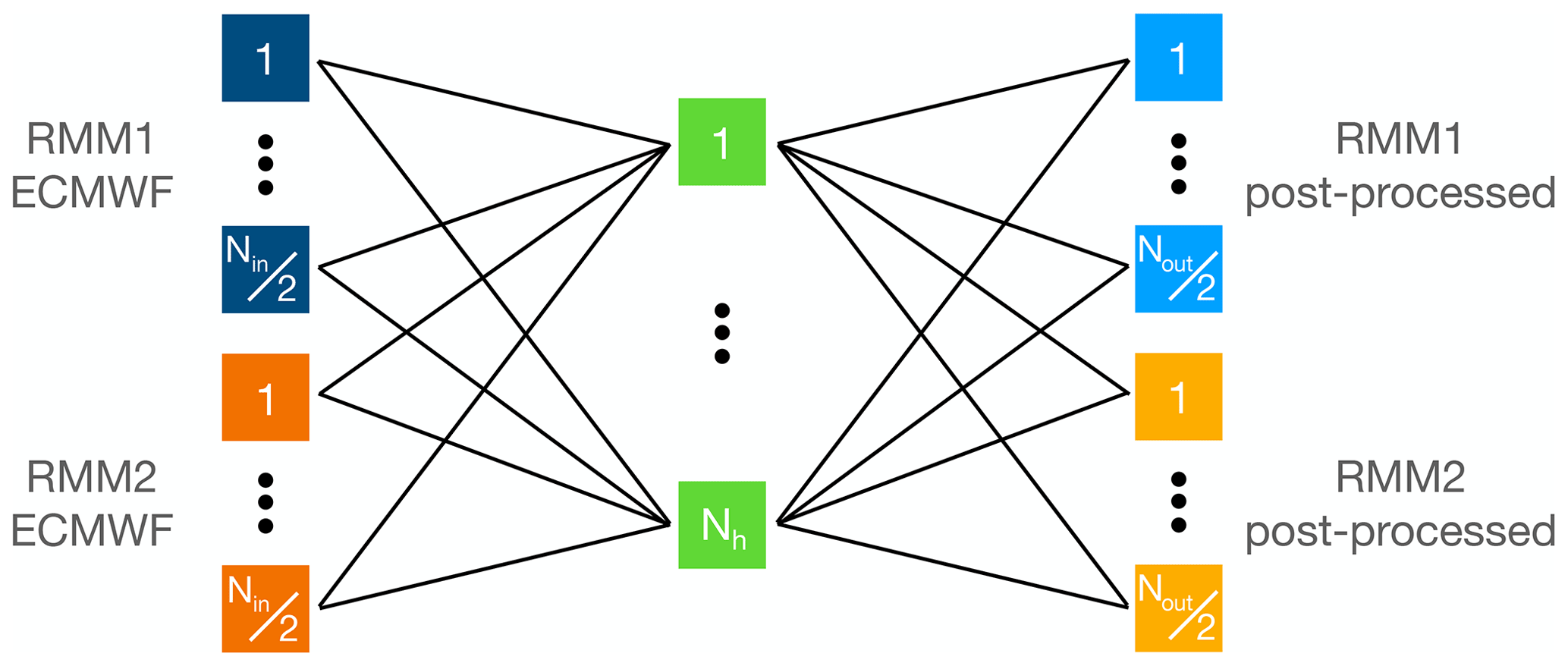
We use an adaptive number of neurons depending on the number of days we want to forecast. The ECMWF reforecasts provide predictions up to a lead time of 46 d for both RMM1 and RMM2, and we build a different network for each lead time. This means that the number of output neurons Nout can fall between 2 and 92 because we use both RMM1 and RMM2.
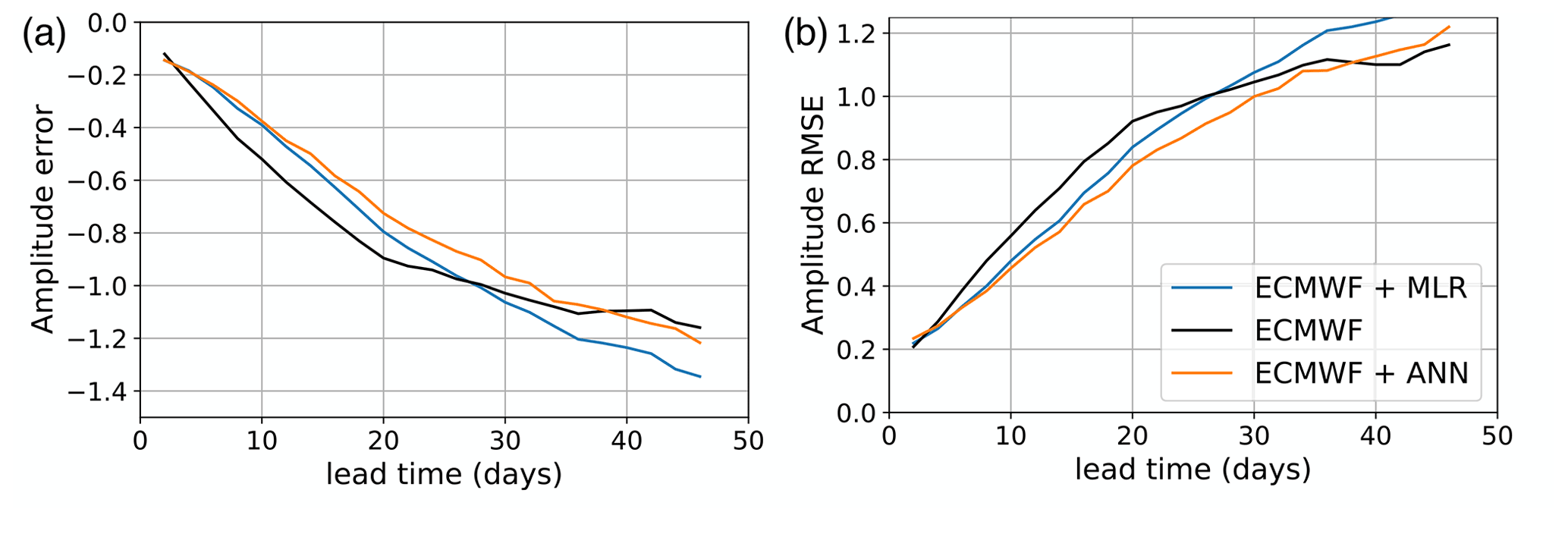
Figure 2(a) MJO amplitude error and (b) amplitude RMSE (b) as a function of the lead time for events starting with an amplitude larger than 1. The color indicates the forecast model, the black line corresponds to the ECMWF forecast, the blue line corresponds to the MLR correction of the ECMWF forecast, and the orange line corresponds to the post-processed ECMWF forecast with an ANN.
After selecting the number of output neurons (which is even and in fact defines our lead time, ), we adapt the number of input Nin and hidden neurons Nh as follows. As input, the networks receive the ECMWF reforecasts, which also limit the number of input neurons Nin in the range between 2 and 92. After training the networks with different Nin, we found the best result is obtained with with an upper limit of 92. This means that for all lead times τ>44, . For lead times larger than 30–35 d, the prediction skill of the models falls below the thresholds of 0.5 and 1.4 imposed by the COR and RMSE, respectively, and thus, the lead times τ>44 are not important to predict. Using all 92 inputs, the prediction skill for short lead times slightly decreases. For simplicity, a fixed number of 92 inputs could also be used. An interpretation of the reason behind this result is that to correct the prediction values for a given day, the future predicted values can help up to some extent. To correct the prediction of a given day, for each RMM we use the predicted values of up to 3 d after that particular day. To avoid overfitting, we want the number of hidden neurons to be relatively small, and for this reason after some tests we select . The training has been performed over 100 epochs which allows us to not overfit the model. The model performance is tested using a walk-forward validation. The procedure is as follows. First, we train the network on an expanding train set and then test its performance on a validation set that contains the N samples that follow the train set. In our case, we found that the optimal minimum number of samples for the train set, out of 2200 available, is 1700 (∼17 years). Then, the train set is extended by 100 samples (∼1 year) for each run and validated on the subsequent 200 samples (∼2 years). This method of walk-forward validation ensures that no information coming from the future of the test set is used to train the model. Other methods to avoid overfitting could also be used, such as early stopping or drop-out.
MLR is the well-known least squares linear regression where the observed RMMs are a linear combination of the ECMWF-predicted RMMs. To compute the MLR we use the Python library scikit-learn (Pedregosa et al., 2011). With MLR we correct the RMMs separately and apply the same walk-forward validation used for the ANNs.
The first part of this section will be devoted to the results obtained for the MJO amplitude and phase. In the second part we present the prediction skill assessment using the COR 0.5 level, and RMSE 1.4 level as metrics, while in the last part of the section we show how the different forecast methods perform for different MJO initial phases.
The results are obtained by training the ANN from 13 June 1999 using a walk-forward validation and averaging the error obtained by testing over different unseen time windows from 5 December 2014 to 29 June 2019. The size of the windows is defined by the selected number of initial days from which the ECMWF forecast starts. Due to the bi-weekly acquisition of ECMWF, this means that each window of 200 points corresponds to 2 years approximately. Each member of the ensemble over which the average is performed corresponds to a test set used for the walk-forward validation. Different sizes of the test set between 100 and 500 samples have been tested, leading to prediction skills that vary sensibly. For this reason, it is important to take into account that results may vary depending on the test set and its size, albeit preserving the same general result: the post-processing corrections improve the ECMWF forecasts.
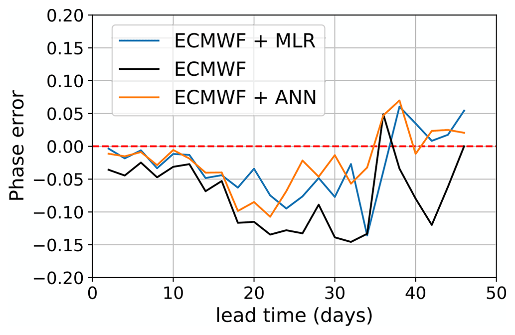
Figure 3MJO phase error for events starting with an amplitude larger than 1. The color indicates the forecast model, the black line corresponds to the ECMWF forecast, the blue line corresponds to the MLR correction of the ECMWF forecast, and the orange line corresponds to the post-processed ECMWF forecast with an ANN.
In Fig. 2, we show the error on the MJO amplitude for events starting with an amplitude larger than 1. We can notice an underestimation of the amplitude as expected (Jiang et al., 2020). Nevertheless, the post-processed amplitudes are closer to the observed ones, with respect to the raw ECMWF forecast. The maximum improvement occurs for a lead time of 28 d when the ECMWF-ANN model has a RMSE similar to the RMSE of the uncorrected ECMWF at a lead time of 20 d.
By the definition of the amplitude error, errors of opposite sign could potentially cancel out resulting in misleading conclusions. For this reason in Fig. 2 we also provide the RMSE of the amplitude error, which shows a similar behavior to before. Both post-processing techniques improve the results, with the ANN bringing the highest benefits in terms of the magnitude of error reduction and the forecasting horizon of the improvement.

Figure 4(a) COR and (b) RMSE as a function of the forecast lead time for events starting with an amplitude larger than 1. The color indicates the forecast model and the red dashed line indicates the prediction skill threshold of COR = 0.5 and RMSE = 1.4. The black line corresponds to the ECMWF forecast, the blue line corresponds to the post-processed ECMWF forecast with MLR, while in orange it is shown the post-processed ECMWF forecast with an ANN.

Figure 5Wheeler–Hendon phase diagram for two different starting dates of the same MJO event, and a 3-week prediction. Panel (a) starting date is 21 November 2018. The MJO enhanced rainfall region travels across the Western Hemisphere and Indian Ocean. Panel (b) starting date is 5 December 2018 and represents a 3-week prediction approaching and traveling over the MC. The rotation of the event in the phase diagram is counter-clockwise, and the dots are included every 7 d, marking the different weeks.
In Fig. 3, we present the MJO phase error. The post-processing techniques provide an improved prediction, during which all three models predict a negative phase. A positive phase error indicates a faster propagating MJO, while a negative error represents a slower propagation. The ECMWF forecast shows an overall slower propagation of the MJO with respect to the observations, and both post-processing corrections provides an increment of the MJO speed prediction. In particular, at the 18 d lead time we can notice an increment of the ECMWF phase error, which MLR and ML tend to correct.
Figure 4, shows the COR and RMSE of the ECMWF ensemble mean forecasts, the MLR, and ANN post-processing. A COR of 0.5 is taken here as baseline for useful prediction skill. We see an improvement of the a prediction skill at the COR = 0.5 level of about 1 d. However, in terms of RMSE, up to a lead time of 4 weeks, neither post-processing technique crosses the RMSE threshold of 1.4, and therefore, they both improve the prediction skill with respect to the raw, unprocessed output of the ECMWF model.
In Fig. 5, we display the comparison between the observations, the ECMWF forecast, and its corrections, in a Wheeler–Hendon phase diagram for two different starting dates of the same MJO event. The dots are marked every 7 d to identify the weeks. In the left panel, the 3-week prediction starts on 21 November 2018 and displays its progression from the Western Hemisphere over the Indian Ocean. It is possible to notice that both post-processing techniques display very similar prediction, with a slightly larger amplitude than ECMWF, closer to the observations for all lead times. In the right panel, the 3-week prediction starts on 5 December 2018 in the Indian Ocean. We can see a drop of accuracy in the ECMWF prediction, and the MLR post-processing, approaching the MC. The ML correction instead preserves a larger amplitude, closer to the observations.
It is also possible to notice that while the speed of the MJO event is well predicted in the left panel, in the right one there is a drop of the MJO speed forecast over the Indian Ocean and MC.
Here we presented an example of a strongly active MJO event, where the corrections clearly improve the ECMWF prediction and it is among the best found. All predictions from 12 December 2014 to 18 June 2019 can be found in Silini (2021b). Looking at these results it is possible to appreciate the general improvement provided by the post-processing corrections.
Finally we study the amplitude error, phase error, COR, and RMSE, as a function of the different initial phases of MJO. As displayed in Fig. 6, applying post-processing methods improves the amplitude error for all initial phases. The MLR provides an improvement with respect to the ECMWF model, but the ML correction leads to the lowest error. Concerning the initial phases, we find the lowest amplitude error when an MJO event starts over the MC, while the largest is found in phase 2, over the Indian Ocean. With the MJO propagating at an average speed of 5 m s−1, events starting in phase 2 will cross the MC in 2–3 weeks time (Kim et al., 2014). The phase error displays a large worsening of the MJO localization prediction, when the forecast starts between the MC and Western Pacific (phase 6–8). This observation is consistent with Fig. 5, where we noticed a drop in the accuracy of the MJO speed prediction over the Indian Ocean and MC. The COR finds its maximum when starting over the MC continent, consistently with the amplitude error. The ML correction has the highest COR except for phase 8, where MLR leads to the highest one. The RMSE is very consistent with the COR, in which we find the minimum in phase 4, with the ML correction having the lowest error, except for phase 8. Overall, we can conclude that the ML post-processing is worth applying especially to reduce the error on the amplitude prediction, while MLR could be useful for a better prediction of the MJO location.
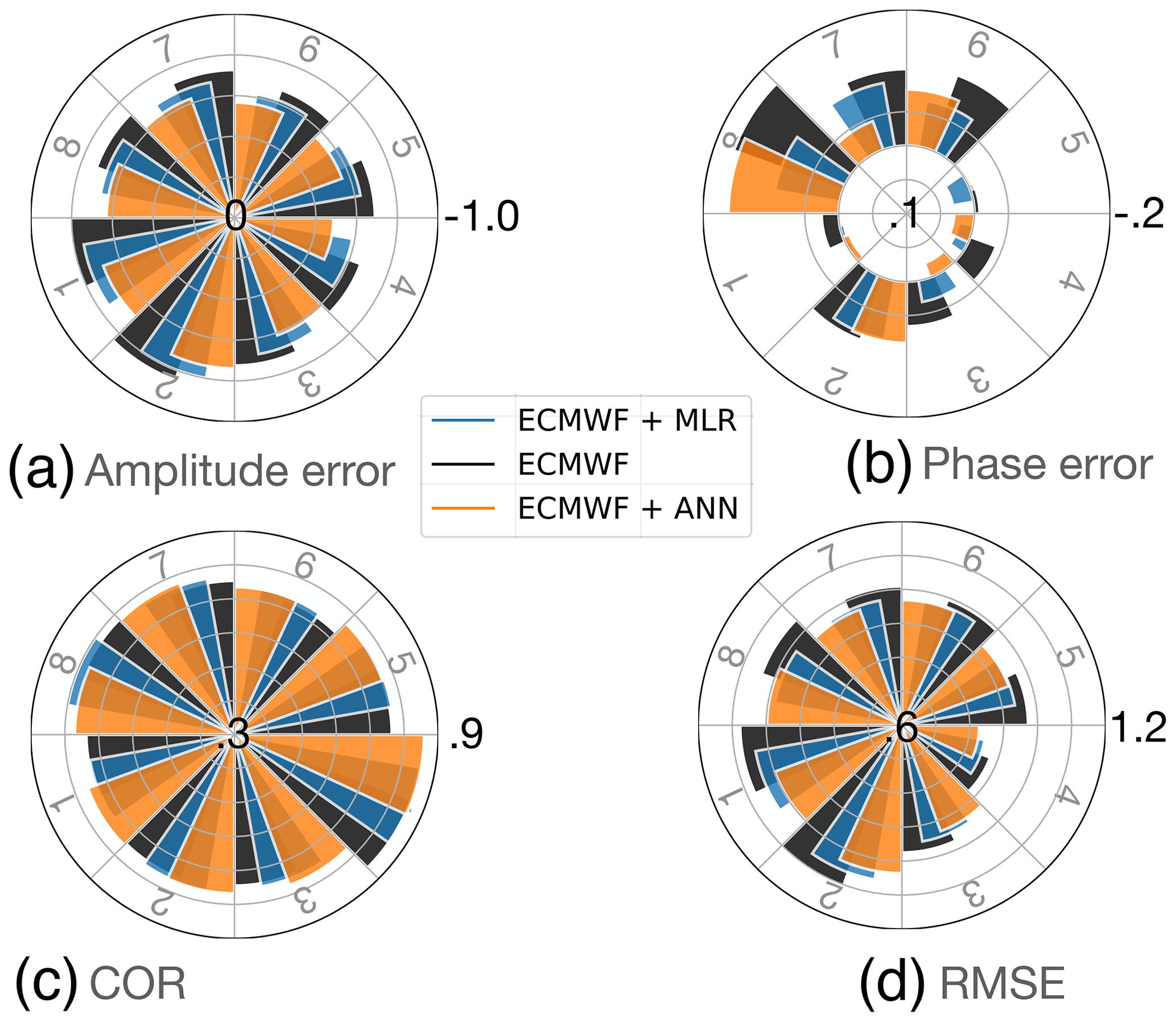
Figure 6(a) Amplitude error, (b) phase error, (c) COR, and (d) RMSE, for the different MJO initial phases, for events starting with an amplitude larger than 1. The plots show the mean for lead times up to 5 weeks. The different colors represent the different prediction methods.
This study confirms the potential of post-processing techniques to reduce the knowledge and bias gap between dynamical model forecasts and observations, providing advancement in MJO prediction.
It is interesting to compare the results presented in Fig. 4 with those reported in Fig. 7 of the Supplement in Kim et al. (2021), keeping in mind that Kim et al. (2021) show the mean BCOR for the eight dynamical models considered. While it can be seen in Fig. 7 in Kim et al. (2021) that for short lead times (up to 2 weeks) a clear improvement with DL post-processing is obtained, the average BCOR for short lead times is quite low compared to the ECMWF prediction. We can also notice that the improvement obtained by Kim et al. (2021) fades away by the fourth week. In contrast, in our case, for short lead times there is no significant improvement (as could be expected, due to the fact that ECMWF model provides the best MJO forecast), but our improvement lasts for longer lead times.
It is also interesting to compare the different post-processing approaches used. While we use a feed-forward neural network (FFNN) architecture, Kim et al. (2021) used a Deep Learning (DL) network, specifically, a long short-term memory (LSTM) network. Having a simpler architecture, FFNNs are usually faster to train and to use than LSTMs. While LSTMs have been proven to be powerful for time sequence modeling, as shown in Kim et al. (2021), in our case we are not trying to predict the future of a time series using its past, but we are trying to improve the predictions.
There are other differences in the architecture of the networks used: we found that to improve the prediction of the RMMs for a day t, the information in the past and future predictions can both help the correction, while in Kim et al. (2021), the future model's predictions (which are available) are not used for the correction. Another difference is that while the algorithm used by Kim et al. (2021) performs an expansion of the system dimensionality (hidden nodes > input nodes), we found good results performing a compression (hidden nodes < input nodes).
Comparing our results to those of post-processing ensemble weather predictions on medium-range timescales (Vannitsem et al., 2021), we find that the general magnitude of improvements over the predictions of the dynamical model is lower. This indicates the increasingly difficult challenge to obtain accurate MJO predictions for longer lead times, likely due to a generally lower predictability and a lower level of useful information that can be learned from the raw ensemble predictions compared to those of many other weather variables on shorter timescales. That said, our results indicating the potential of modern DL methods to improve over classical statistical approaches are well in line with the findings for medium-range post-processing (Rasp and Lerch, 2018; Vannitsem et al., 2021; Haupt et al., 2021).
We employed a MLR and a ML algorithm to perform a post-processing correction of the prediction of the dynamical model that currently holds the highest MJO prediction skill (Jiang et al., 2020), developed by ECMWF.
The largest improvement is found in the MJO amplitude and phase individually, which decreases the underestimation of the amplitude, providing a more accurate predicted geographical location of the MJO. The amplitude and phase estimation are improved for all lead times up to 5 weeks.
We obtained an improved prediction skill of about 1 d for a COR of 0.5.
Plotting the forecasts in a Wheeler–Hendon phase diagram we found an improvement in predicting the MJO propagation, notably across the MC, which helps overcome the MC barrier.
Considering the results obtained for each initial MJO phase, we found that both post-processing tools improve the prediction, with the ML correction being the best.
The ML technique provides an improvement over MLR for all initial phases except phase 8. In the case of phase forecast it might be also sufficient to use MLR instead of ML. This suggests a predominance of linear corrections to improve the MJO phase forecast.
Due to the influence of the initial phase, amplitude, and season on the prediction skill, it would be ideal to train the ANNs for the different initial conditions, but this is not possible because of the limited data that are available for the training.
As future work, it would be interesting to test a stochastic approach to post-processing (as in Rasp and Lerch, 2018), which would allow us to obtain a probabilistic forecast. A promising path to further reduce the prediction error is to include other informative variables as inputs to the ANNs in conjunction with the ECMWF predictions. These additional variables should be carefully selected using methods of causal inference such as well-known Granger causality (Granger, 1969), transfer entropy (Schreiber, 2000; Paluš and Vejmelka, 2007) and convergent cross mapping (Sugihara et al., 2012), or the recently proposed pseudo transfer entropy (Silini and Masoller, 2021; Silini et al., 2022).
Although the improvement provided by the MLR and ML techniques, a post-processing method will always strongly rely on the accuracy of the dynamical model's forecasts. For this reason, it is crucial to work on both dynamical models and machine learning methods to progress.
The Keras TensorFlow (Abadi et al., 2015) trained FFNN can be found at https://doi.org/10.5281/zenodo.5801453 (Silini, 2021a). The RMM data and the ECMWF reforecasts can be freely downloaded from ECMWF (2021).
RS performed the analysis and prepared the figures. RS, SL, and NM designed the study. All authors discussed the results and wrote and reviewed the paper.
The contact author has declared that none of the authors has any competing interests.
Publisher's note: Copernicus Publications remains neutral with regard to jurisdictional claims in published maps and institutional affiliations.
The authors thank Linus Magnusson for providing access to the data. This work received funding from the European Union's Horizon 2020 research and innovation program under the Marie Skłodowska–Curie Actions agreement no. 813844. Cristina Masoller also acknowledges funding by the Spanish Ministerio de Ciencia, Innovacion y Universidades (PGC2018-099443-B-I00) and the ICREA ACADEMIA program of Generalitat de Catalunya. Sebastian Lerch acknowledges support by the Vector Stiftung through the Young Investigator Group “Artificial Intelligence for Probabilistic Weather Forecasting”.
This research has been supported by the H2020 Marie Skłodowska–Curie Actions (grant no. 813844), the Vector Stiftung (Artificial Intelligence for Probabilistic Weather Forecasting), the Institució Catalana de Recerca i Estudis Avançats, and the Ministerio de Ciencia, Innovación y Universidades (grant no. PID2021-123994NB-C21).
This paper was edited by Andrey Gritsun and reviewed by two anonymous referees.
Abadi, M., Agarwal, A., Barham, P., Brevdo, E., Chen, Z., Citro, C., Corrado, G. S., Davis, A., Dean, J., Devin, M., Ghemawat, S., Goodfellow, I., Harp, A., Irving, G., Isard, M., Jia, Y., Jozefowicz, R., Kaiser, L., Kudlur, M., Levenberg, J., Mané, D., Monga, R., Moore, S., Murray, D., Olah, C., Schuster, M., Shlens, J., Steiner, B., Sutskever, I., Talwar, K., Tucker, P., Vanhoucke, V., Vasudevan, V., Viégas, F., Vinyals, O., Warden, P., Wattenberg, M., Wicke, M., Yu, Y., and Zheng, X.: TensorFlow: Large-Scale Machine Learning on Heterogeneous Systems, http://tensorflow.org/ (last access: 15 July 2022), 2015. a
Alvarez, M. S., Vera, C. S., and Kiladis, G. N.: MJO Modulating the Activity of the Leading Mode of Intraseasonal Variability in South America, Atmosphere, 8, 232, https://doi.org/10.3390/atmos8120232, 2017. a
Barrett, B. S., Densmore, C. R., Ray, P., and Sanabia, E. R.: Active and weakening MJO events in the Maritime Continent, Clim. Dynam., 57, 157–172, https://doi.org/10.1007/s00382-021-05699-8, 2021. a
Bergman, J. W., Hendon, H. H., and Weickmann, K. M.: Intraseasonal Air–Sea Interactions at the Onset of El Niño, J. Climate, 14, 1702–1719, 2001. a
Camargo, S. J., Wheeler, M. C., and Sobel, A. H.: Diagnosis of the MJO Modulation of Tropical Cyclogenesis Using an Empirical Index, J. Atmos. Sci., 66, 3061–3074, https://doi.org/10.1175/2009JAS3101.1, 2009. a
Dasgupta, P., Metya, A., Naidu, C. V., Singh, M., and Roxy, M. K.: Exploring the long-term changes in the Madden Julian Oscillation using machine learning, Scient. Rep., 10, 18567, https://doi.org/10.1038/s41598-020-75508-5, 2020. a
Díaz, N., Barreiro, M., and Rubido, N.: Intraseasonal Predictions for the South American Rainfall Dipole, Geophys. Res. Lett., 47, e2020GL089985, https://doi.org/10.1029/2020GL089985, 2020. a
Dijkstra, H. A., Petersik, P., Hernández-García, E., and López, C.: The Application of Machine Learning Techniques to Improve El Niño Prediction Skill, Front. Phys., 7, 153, https://doi.org/10.3389/fphy.2019.00153, 2019. a
ECMWF: ECMWF RMM reforecasts data, https://acquisition.ecmwf.int/ecpds/data/list/RMMS/ecmwf/reforecasts/, last access: February 2021. a, b, c
Ferranti, L., Magnusson, L., Vitart, F., and Richardson, D. S.: How far in advance can we predict changes in large-scale flow leading to severe cold conditions over Europe?, Q. J. Roy. Meteorol. Soc., 144, 1788–1802, https://doi.org/10.1002/qj.3341, 2018. a
Fowler, M. D. and Pritchard, M. S.: Regional MJO Modulation of Northwest Pacific Tropical Cyclones Driven by Multiple Transient Controls, Geophys. Res. Lett., 47, e2020GL087148, https://doi.org/10.1029/2020GL087148, 2020. a
Gagne II, D. J., Christensen, H. M., Subramanian, A. C., and Monahan, A. H.: Machine Learning for Stochastic Parameterization: Generative Adversarial Networks in the Lorenz'96 Model, J. Adv. Model. Earth Syst., 12, e2019MS001896, https://doi.org/10.1029/2019MS001896, 2020. a
Granger, C. W. .: Investigating Causal Relations by Econometric Models and Cross-spectral Methods, Econometrica, 37, 424–459, 1969. a
Ham, Y.-G., Kim, J.-H., and Luo, J.-J.: Deep learning for multi-year ENSO forecasts, Nature, 573, 568–572, https://doi.org/10.1038/s41586-019-1559-7, 2019. a
Haupt, S. E., Chapman, W., Adams, S. V., Kirkwood, C., Hosking, J. S., Robinson, N. H., Lerch, S., and Subramanian, A. C.: Towards implementing artificial intelligence post-processing in weather and climate: proposed actions from the Oxford 2019 workshop, Philos. T. Roy. Soc. A, 379, 20200091, https://doi.org/10.1098/rsta.2020.0091, 2021. a, b
Jiang, X., Adames, A. F., Kim, D., Maloney, E. D., Lin, H., Kim, H., Zhang, C., DeMott, C. A., and Klingaman, N. P.: Fifty Years of Research on the Madden–Julian Oscillation: Recent Progress, Challenges, and Perspectives, J. Geophys. Res.-Atmos., 125, e2019JD030911, https://doi.org/10.1029/2019JD030911, 2020. a, b, c, d, e
Kim, H., Vitart, F., and Waliser, D. E.: Prediction of the Madden–Julian Oscillation: A Review, J. Climate, 31, 9425–9443, https://doi.org/10.1175/JCLI-D-18-0210.1, 2018. a
Kim, H., Ham, Y. G., Joo, Y. S., and Son, S. W.: Deep learning for bias correction of MJO prediction, Nat. Commun., 12, 3087, https://doi.org/10.1038/s41467-021-23406-3, 2021. a, b, c, d, e, f, g, h, i, j
Kim, H.-M., Webster, P. J., Toma, V. E., and Kim, D.: Predictability and Prediction Skill of the MJO in Two Operational Forecasting Systems, J. Climate, 27, 5364–5378, https://doi.org/10.1175/JCLI-D-13-00480.1, 2014. a
Kim, H.-M., Kim, D., Vitart, F., Toma, V. E., Kug, J.-S., and Webster, P. J.: MJO Propagation across the Maritime Continent in the ECMWF Ensemble Prediction System, J.Climate, 29, 3973–3988, https://doi.org/10.1175/JCLI-D-15-0862.1, 2016. a
Klotzbach, P. J.: On the Madden–Julian Oscillation–Atlantic Hurricane Relationship, J. Climate, 23, 282–293, https://doi.org/10.1175/2009JCLI2978.1, 2010. a
Lau, W. K. M. and Waliser, D. E.: Predictability and forecasting, Springer, Berlin, Heidelberg, https://doi.org/10.1007/978-3-642-13914-7_12, 2011. a
Lin, H., Brunet, G., and Derome, J.: Forecast Skill of the Madden–Julian Oscillation in Two Canadian Atmospheric Models, Mon. Weather Rev., 136, 4130–4149, https://doi.org/10.1175/2008MWR2459.1, 2008. a
Madden, R. A. and Julian, P. R.: Detection of a 40–50 Day Oscillation in the Zonal Wind in the Tropical Pacific, J. Atmos. Sci., 28, 702 –708, https://doi.org/10.1175/1520-0469(1971)028<0702:DOADOI>2.0.CO;2, 1971. a
Madden, R. A. and Julian, P. R.: Description of Global-Scale Circulation Cells in the Tropics with a 40–50 Day Period, J. Atmos. Sci., 29, 1109–1123, https://doi.org/10.1175/1520-0469(1972)029<1109:DOGSCC>2.0.CO;2, 1972. a
Martin, Z. K., Barnes, E. A., and Maloney, E. D.: Using simple, explainable neural networks to predict the Madden-Julian oscillation, Earth and Space Science Open Archive, https://doi.org/10.1002/essoar.10507439.1, 2021a. a
Martin, Z. K., Son, S.-W., Butler, A., Hendon, H., Kim, H., Sobel, A., Yoden, S., and Zhang, C.: The influence of the quasi-biennial oscillation on the Madden-Julian oscillation, Nature Rev. Earth Environ., 2, 477–489, https://doi.org/10.1038/s43017-021-00173-9, 2021b. a
McGovern, A., Lagerquist II, R. D. J. G., Jergensen, G. E., Elmore, K. L., Homeyer, C. R., and Smith, T.: Making the Black Box More Transparent: Understanding the Physical Implications of Machine Learning, B. Am. Meteorol. Soc., 100, 2175–2199, https://doi.org/10.1175/BAMS-D-18-0195.1, 2019. a
Nooteboom, P. D., Feng, Q. Y., López, C., Hernández-García, E., and Dijkstra, H. A.: Using network theory and machine learning to predict El Niño, Earth Syst. Dynam., 9, 969–983, https://doi.org/10.5194/esd-9-969-2018, 2018. a
O'Gorman, P. A. and Dwyer, J. G.: Using Machine Learning to Parameterize Moist Convection: Potential for Modeling of Climate, Climate Change, and Extreme Events, J. Adv. Model. Earth Syst., 10, 2548–2563, https://doi.org/10.1029/2018MS001351, 2018. a
Paluš, M. and Vejmelka, M.: Directionality of coupling from bivariate time series: How to avoid false causalities and missed connections, Phys. Rev. E, 75, 056211, https://doi.org/10.1103/PhysRevE.75.056211, 2007. a
Pedregosa, F., Varoquaux, G., Gramfort, A., Michel, V., Thirion, B., Grisel, O., Blondel, M., Prettenhofer, P., Weiss, R., Dubourg, V., Vanderplas, J., Passos, A., Cournapeau, D., Brucher, M., Perrot, M., and Duchesnay, E.: Scikit-learn: Machine Learning in Python, J. Mach. Learn. Res., 12, 2825–2830, 2011. a
Rashid, H. A., Hendon, H. H., Wheeler, M. C., and Alves, O.: Prediction of the Madden–Julian oscillation with the POAMA dynamical prediction system, Clim. Dynam., 36, 649–661, https://doi.org/10.1007/s00382-010-0754-x, 2011. a, b, c, d
Rasp, S. and Lerch, S.: Neural networks for postprocessing ensemble weather forecasts, Mon. Weather Rev., 146, 3885–3900, https://doi.org/10.1175/MWR-D-18-0187.1, 2018. a, b, c
Scheuerer, M., Switanek, M. B., Worsnop, R. P., and Hamill, T. M.: Using Artificial Neural Networks for Generating Probabilistic Subseasonal Precipitation Forecasts over California, Mon. Weather Rev., 148, 3489–3506, https://doi.org/10.1175/MWR-D-20-0096.1, 2020. a
Schreiber, T.: Measuring Information Transfer, Phys. Rev. Lett., 85, 461–464, 2000. a
Silini, R.: MJO post-processing artificial neural networks, Zenodo [code], https://doi.org/10.5281/zenodo.5801453, 2021a. a
Silini, R.: Wheeler–Hendon phase diagrams, Zenodo [video supplement], https://doi.org/10.5281/zenodo.5801415, 2021b. a
Silini, R. and Masoller, C.: Fast and effective pseudo transfer entropy for bivariate data-driven causal inference, Scient. Rep., 11, 1–13, 2021. a
Silini, R., Barreiro, M., and Masoller, C.: Machine learning prediction of the Madden-Julian Oscillation, npj Clim. Atmos. Sci., 4, 57, https://doi.org/10.1038/s41612-021-00214-6, 2021. a, b
Silini, R., Tirabassi, G., Barreiro, M., Ferranti, L., and Masoller, C.: Assessing causal dependencies in climatic indices, Clim. Dynam., in review, 2022. a
Sugihara, G., May, R., Ye, H., Hsieh, C. H., Deyle, E., Fogarty, M., and Munch, S.: Detecting causality in complex ecosystems, Science, 338, 496–500, https://doi.org/10.1126/science.1227079, 2012. a
Taraphdar, S., Zhang, F., Leung, L. R., Chen, X., and Pauluis, O. M.: MJO affects the Monsoon Onset Timing Over the Indian Region, Geophys. Res. Lett., 45, 10011–10018, https://doi.org/10.1029/2018GL078804, 2018. a
Tseng, K.-C., Barnes, E. A., and Maloney, E.: The Importance of Past MJO Activity in Determining the Future State of the Midlatitude Circulation, J. Climate, 33, 2131–2147, https://doi.org/10.1175/JCLI-D-19-0512.1, 2020. a
Ungerovich, M., Barreiro, M., and Masoller, C.: Influence of Madden–Julian Oscillation on extreme rainfall events in Spring in southern Uruguay, Int. J. Climatol., 41, 3339–3351, https://doi.org/10.1002/joc.7022, 2021. a
Vannitsem, S., Bremnes, J. B., Demaeyer, J., Evans, G. R., Flowerdew, J., Hemri, S., Lerch, S., Roberts, N., Theis, S., Atencia, A., Bouallègue, Z. B., Bhend, J., Dabernig, M., Cruz, L D., Hieta, L., Mestre, O., Moret, L., Plenković, I., Schmeits, M., Taillardat, M., den Bergh, J. V., Schaeybroeck, B. V., Whan, K., and Ylhaisi, J.: Statistical Postprocessing for Weather Forecasts: Review, Challenges, and Avenues in a Big Data World, B. Am. Meteorol. Soc., 102, E681–E699, https://doi.org/10.1175/BAMS-D-19-0308.1, 2021. a, b, c
Vitart, F.: Impact of the Madden Julian Oscillation on tropical storms and risk of landfall in the ECMWF forecast system, Geophys. Res. Lett., 36, L15802, https://doi.org/10.1029/2009GL039089, 2009. a
Wang, S., Tippett, M. K., Sobel, A. H., Martin, Z. K., and Vitart, F.: Impact of the QBO on Prediction and Predictability of the MJO Convection, J. Geophys. Res.-Atmos., 124, 11766–11782, https://doi.org/10.1029/2019JD030575, 2019. a
Wheeler, M. C. and Hendon, H. H.: An All-Season Real-Time Multivariate MJO Index: Development of an Index for Monitoring and Prediction, Mon. Weather Rev., 132, 1917–1932, https://doi.org/10.1175/1520-0493(2004)132<1917:AARMMI>2.0.CO;2, 2004. a
Wheeler, M. C., Hendon, H. H., Cleland, S., Meinke, H., and Donald, A.: Impacts of the Madden-Julian Oscillation on Australian Rainfall and Circulation, J. Climate, 22, 1482–1498, https://doi.org/10.1175/2008JCLI2595.1, 2009. a
Wu, C.-H. and Hsu, H.-H.: Topographic Influence on the MJO in hte Maritime Continent, J. Climate, 22, 5433–5448, https://doi.org/10.1175/2009JCLI2825.1, 2009. a
Wu, J. and Jin, F.-F.: Improving the MJO Forecast of S2S Operation Models by Correcting Their Biases in Linear Dynamics, Geophys. Res. Lett., 48, e2020GL091930, https://doi.org/10.1029/2020GL091930, 2021. a
Zhang, C., Gottschalck, J., Maloney, E. D., Moncrieff, M. W., Vitart, F., Waliser, D. E., Wang, B., and Wheeler, M. C.: Cracking the MJO nut, Geophys. Res. Lett., 40, 1223–1230, https://doi.org/10.1002/grl.50244, 2013. a, b