the Creative Commons Attribution 4.0 License.
the Creative Commons Attribution 4.0 License.
 | 29 Jul 2022
Estimating the lateral transfer of organic carbon through the European river network using a land surface model
Ronny Lauerwald
Pierre Regnier
Philippe Ciais
Kristof Van Oost
Victoria Naipal
Bertrand Guenet
Wenping Yuan
Lateral carbon transport from soils to the ocean through rivers has been acknowledged as a key component of the global carbon cycle, but it is still neglected in most global land surface models (LSMs). Fluvial transport of dissolved organic carbon (DOC) and CO2 has been implemented in the ORCHIDEE LSM, while erosion-induced delivery of sediment and particulate organic carbon (POC) from land to river was implemented in another version of the model. Based on these two developments, we take the final step towards the full representation of biospheric carbon transport through the land–river continuum. The newly developed model, called ORCHIDEE-Clateral, simulates the complete lateral transport of water, sediment, POC, DOC, and CO2 from land to sea through the river network, the deposition of sediment and POC in the river channel and floodplains, and the decomposition of POC and DOC in transit. We parameterized and evaluated ORCHIDEE-Clateral using observation data in Europe. The model explains 94 %, 75 %, and 83 % of the spatial variations of observed riverine water discharges, bankfull water flows, and riverine sediment discharges in Europe, respectively. The simulated long-term average total organic carbon concentrations and DOC concentrations in river flows are comparable to the observations in major European rivers, although our model generally overestimates the seasonal variation of riverine organic carbon concentrations. Application of ORCHIDEE-Clateral for Europe reveals that the lateral carbon transfer affects land carbon dynamics in multiple ways, and omission of this process in LSMs may lead to an overestimation of 4.5 % in the simulated annual net terrestrial carbon uptake over Europe. Overall, this study presents a useful tool for simulating large-scale lateral carbon transfer and for predicting the feedbacks between lateral carbon transfer and future climate and land use changes.
- Article
(10875 KB) - Full-text XML
-
Supplement
(4885 KB) - BibTeX
- EndNote


Lateral transfer of organic carbon along the land–river–ocean continuums, involving both spatial redistribution of terrestrial organic carbon and the vertical land–atmosphere carbon exchange, has been acknowledged as a key component of the global carbon cycle (Ciais et al., 2013, 2021; Drake et al., 2018; Regnier et al., 2013, 2022). Erosion of soils and the associated organic carbon, but also leaching of soil dissolved organic carbon (DOC), represent a non-negligible leak in the terrestrial carbon budget and a substantial source of allochthonous organic carbon to inland waters and oceans (Battin et al., 2009; Cole et al., 2007; Raymond et al., 2013; Regnier et al., 2013). As a result of soil aggregate breakdown and desorption, the accelerated mineralization of these eroded and leached soil carbon loads leads to considerable CO2 emission to the atmosphere (Chappell et al., 2016; Lal, 2003; Van Hemelryck et al., 2011). Meanwhile, the organic carbon that is redeposited and buried in floodplains and lakes might be preserved for a long time, thus creating a CO2 sink (Stallard, 1998; Van Oost et al., 2007; Wang et al., 2010; Hoffmann, 2022). In addition, lateral redistribution of soil material can alter land–atmosphere CO2 fluxes indirectly by affecting soil nutrient availability, terrestrial vegetation productivity, and physiochemical properties of inland and coastal waters (Beusen et al., 2005; Vigiak et al., 2017).
Although the important role of lateral carbon transfer in the global carbon cycle has been widely recognized, to date, the estimates of land carbon loss to inland waters, the fate of the terrestrial organic carbon within inland waters, and the net effect of lateral carbon transfer on land–atmosphere CO2 fluxes remain largely uncertain (Berhe et al., 2007; Doetterl et al., 2016; Lal, 2003; Stallard, 1998; Z. Wang et al., 2014; Zhang et al., 2014). Existing estimates of global carbon loss from soils to inland waters vary from 1.1 to 5.1 Pg (=1015 g) C per year (yr−1) (Cole et al., 2007; Drake et al., 2018), and the estimated net impact of global lateral carbon redistribution on the land–atmosphere carbon budget ranges from an uptake of atmospheric CO2 by 1 Pg C yr−1 to a land CO2 emission of 1 Pg C yr−1 (Lal, 2003; Stallard, 1998; Van Oost et al., 2007; Wang et al., 2017; Regnier et al., 2022). A reliable model which is able to explicitly simulate the lateral carbon flux along the land–river continuum and also the interactions between these lateral fluxes and the comprehensive terrestrial carbon cycle would thus be necessary for projecting changes in the global carbon cycle more accurately.
Global land surface models (LSMs) are important tools to simulate the feedbacks between terrestrial carbon cycle, increasing atmospheric CO2, and climate and land use change. However, the lateral carbon transfer, especially for particulate organic carbon (POC), is still missing or incompletely represented in existing LSMs (Lauerwald et al., 2017, 2020; Lugato et al., 2016; Naipal et al., 2020; Nakhavali et al., 2021; Tian et al., 2015). It has been hypothesized that the exclusion of lateral carbon transfer in LSMs implies a significant bias in the simulated global land carbon budget (Ciais et al., 2013, 2021; Janssens et al., 2003). For instance, the study of Nakhavali et al. (2021) suggested that about 15 % of the global terrestrial net ecosystem production is exported to inland waters as leached DOC. Lauerwald et al. (2020) showed that the omission of lateral DOC transfer in LSMs might lead to significant underestimation (8.6 %) of the net uptake of atmospheric carbon in the Amazon basin, while terrestrial carbon storage changes in response to the increasing atmospheric CO2 concentrations were overestimated.
Over the past decade, a number of LSMs have been developed which represent leaching of DOC from soils (Nakhavali et al., 2021; Kicklighter et al., 2013) or the full transport of DOC through the land–river continuum (Lauerwald et al., 2017; Tian et al., 2015). However, the erosion-induced transport of soil POC, which has also been reported to be able to strongly affect the carbon balance of terrestrial ecosystems (Lal, 2003; Van Oost et al., 2007; Tian et al., 2015), is still not represented or is poorly represented in LSMs. The explicit simulation of the complete transport process of POC at large spatial scales is still a major challenge due to the complexity of the processes involved, including erosion-induced sediment and POC delivery to rivers, deposition of sediment and POC in river channels and floodplains, re-detachment of the previously deposited sediments and POC, decomposition and transformation of POC in riverine and flooding waters, and the changes in the soil profile caused by erosion and deposition (Doetterl et al., 2016; Naipal et al., 2020; Zhang et al., 2020).
Several recent model developments have led to the implementation of the lateral transfer of POC in large-scale LSMs. Despite this, there are still some inevitable limitations in these implementations. The Dynamic Land Ecosystem Model (DLEM v2.0, Tian et al., 2015) is able to simulate the erosion-induced POC loss from soil to river and the transport and decomposition of POC in river networks. However, it does not represent the POC deposition in floodplains or the impacts of soil erosion and floodplain deposition on the vertical profiles of soil organic carbon (SOC). The Carbon Erosion DYNAMics model (CE-DYNAM, Naipal et al., 2020) simulates erosion of SOC and its redeposition on the toe slope or floodplains, transport of POC along river channels, and the impact on SOC dynamics at the eroding and deposition sites. However, running at an annual timescale, it mostly addresses the centennial timescale and does not represent deposition and decomposition of POC in river channels. Moreover, CE-DYNAM was only applied over the Rhine catchment and has not been fully coupled into a land surface model, therefore excluding the feedbacks of soil erosion on the fully coupled land and aquatic carbon cycles. There are of course more dedicated hydrology and soil erosion models that explicitly simulate the complete transport, deposition, and decomposition processes of POC in small river basins (e.g., Jetten et al., 2003; Nearing et al., 1989; Neitsch et al., 2011). However, it is difficult to apply these models at large spatial scales (e.g., continental or global scale) due to the limited availability of forcing data (e.g., geometric attributes of river channel), suitable model parameterization, and computational capacity. Moreover, these models have limited capability to represent the full terrestrial C cycle in response to climate change, increasing atmospheric CO2, and land use change. Therefore, basin-scale models are not an option to assess the impact of soil erosion on the large-scale terrestrial C budget in response to global changes.
Here we describe the development, application, and evaluation of a new branch of the ORCHIDEE LSM (Krinner et al., 2005), hereafter ORCHIDEE-Clateral, that can be used to simulate the complete lateral transfer processes of water, sediment, POC, and DOC along the land–river–ocean continuum at large spatial scale (e.g., continental and global scale). In previous studies, the leaching and fluvial transfer of DOC and the erosion-induced delivery of sediment and POC from upland soil to river network have been implemented in two different branches of the ORCHIDEE LSM (i.e., ORCHILEAK, Lauerwald et al., 2017, and ORCHIDEE-MUSLE, Zhang et al., 2020). For this new branch, we first merged these two branches and subsequently implemented the fluvial transfer of sediment and POC in the coupled model. ORCHIDEE-Clateral is calibrated and evaluated using observation data on runoff, bankfull flow, and riverine loads, as well as concentrations of sediment, POC, and DOC across Europe. By applying the calibrated model at the European scale, we estimate the magnitude and spatial distribution of the lateral carbon transfer in European catchments during the period 1901–2014, as well as the potential impacts of lateral carbon transfer on the land carbon balance. Comparing simulation results to those of an alternative simulation run with lateral displacement of C deactivated, we finally quantify the biases in simulated land C budgets that arise ignoring the lateral transfers of C along the land–river continuum.
2.1 ORCHIDEE land surface model
The ORCHIDEE LSM comprehensively simulates the cycling of energy, water, and carbon in terrestrial ecosystems (Krinner et al., 2005). The hydrological processes (e.g., rainfall interception, evapotranspiration, and soil water dynamics) and plant photosynthesis in ORCHIDEE are simulated at a time step of 30 min. The carbon cycle processes (e.g., maintenance and growth respiration, carbon allocation, litter decomposition, SOC dynamics, plant phenology and mortality) are simulated at daily time step. In its default configuration, ORCHIDEE represents 13 land cover types, with one for bare soil and 12 for lands covered by vegetation (eight types of forests, two types of grasslands, two types of croplands). Given appropriate land cover maps and parametrization, the number of plant functional types (PFTs) to be represented can, however, be adapted (Zhang et al., 2020).
Our previous implementations of lateral DOC transfer (Lauerwald et al., 2017) and POC delivery from upland to river network (Zhang et al., 2020) were both based on the ORCHIDEE branch ORCHIDEE-SOM (Camino-Serrano et al., 2018, Fig. S1), which provides a depth-dependent description of the water and carbon dynamics in the soil column. Specifically, the vertical soil profile in ORCHIDEE-SOM is described by an 11-layer discretization of a 2 m soil column (Camino-Serrano et al., 2018). Water flows between adjacent soil layers are simulated using the Fokker–Planck equation that resolves water diffusion in non-saturated conditions (Campoy et al., 2013; Guimberteau et al., 2018). Free gravitational drainage occurs in the lowest soil layer when actual soil water content is higher than the residual water content (Campoy et al., 2013). Following the CENTURY model (Parton et al., 1988), ORCHIDEE-SOM represents two litter pools (metabolic and structural) and three SOC pools (active, slow, and passive) that differ in their respective turnover times. The decomposition of each carbon pool is calculated by first-order kinetics based on the corresponding turnover time, soil moisture and temperature as controlling factors, and the priming effects of fresh organic matter (Guenet et al., 2016, 2018). Soil DOC is represented by a labile and a refractory DOC pool, with a high and low turnover rate, respectively. Each DOC pool may be in the soil solution or adsorbed on the mineral matrix. The products of litter and SOC decomposition enter the free DOC pool, which in turn is decomposed following first-order kinetics (Kalbitz et al., 2003) and returns back to SOC. Adsorption and desorption of DOC follow an equilibrium distribution coefficient calculated from soil clay and pH. Free DOC can be transported with the water flux simulated by the soil hydrological module of ORCHIDEE. However, DOC adsorbed to soil minerals can neither be decomposed nor transported (Camino-Serrano et al., 2018). All the described processes occur within each soil layer. At each time step, “the flux of DOC leaving the soil is calculated by multiplying DOC concentrations in soil solution with the runoff (surface layer) and drainage (bottom layer) flux simulated by the hydrological module” (Camino-Serrano et al., 2018, p. 939). More detailed information about the simulation of soil hydrological and biogeochemical processes in ORCHIDEE-SOM can be found in Guenet et al. (2016) and Camino-Serrano et al. (2018).
2.1.1 Lateral transfer of DOC and CO2
Lateral transfer of DOC and dissolved CO2 from land to ocean through river network has been implemented in ORCHILEAK (Lauerwald et al., 2017), an ORCHIDEE branch developed from ORCHIDEE-SOM (Fig. S1). The method used in ORCHILEAK to simulate the adsorption, desorption, production, consumption, and transport of DOC within the soil column, as well as DOC export from the soil column with surface runoff and drainage, is similar to that used in ORCHIDEE-SOM. Besides the decomposition of SOC and litter, ORCHILEAK also represents the contribution of wet and dry deposition to soil DOC via throughfall. The direct DOC input from rainfall to aquatic DOC pools is simulated based on the DOC concentration in rainfall and the area fraction of stream and flooding waters in each basin (Table 1). Note that the maximum area fractions of river surface and floodplain in each basin (i.e., each grid cell in this study) are derived from high-resolution topographic data (Table 1). As it is difficult to explicitly represent all real river channels in a global land surface model (due to the limit of computing efficiency of current computers), we assume that there is one virtual river channel in each pixel. The surface area of this virtual river is the sum of all real rivers, and the flow direction of this virtual is assumed to be same to the largest real river (Lauerwald et al., 2015).
Table 1List of forcing data needed to run ORCHIDEE-Clateral and the data used to evaluate the simulation results. Sres and Tres are the spatial and temporal resolution of the forcing data, respectively.
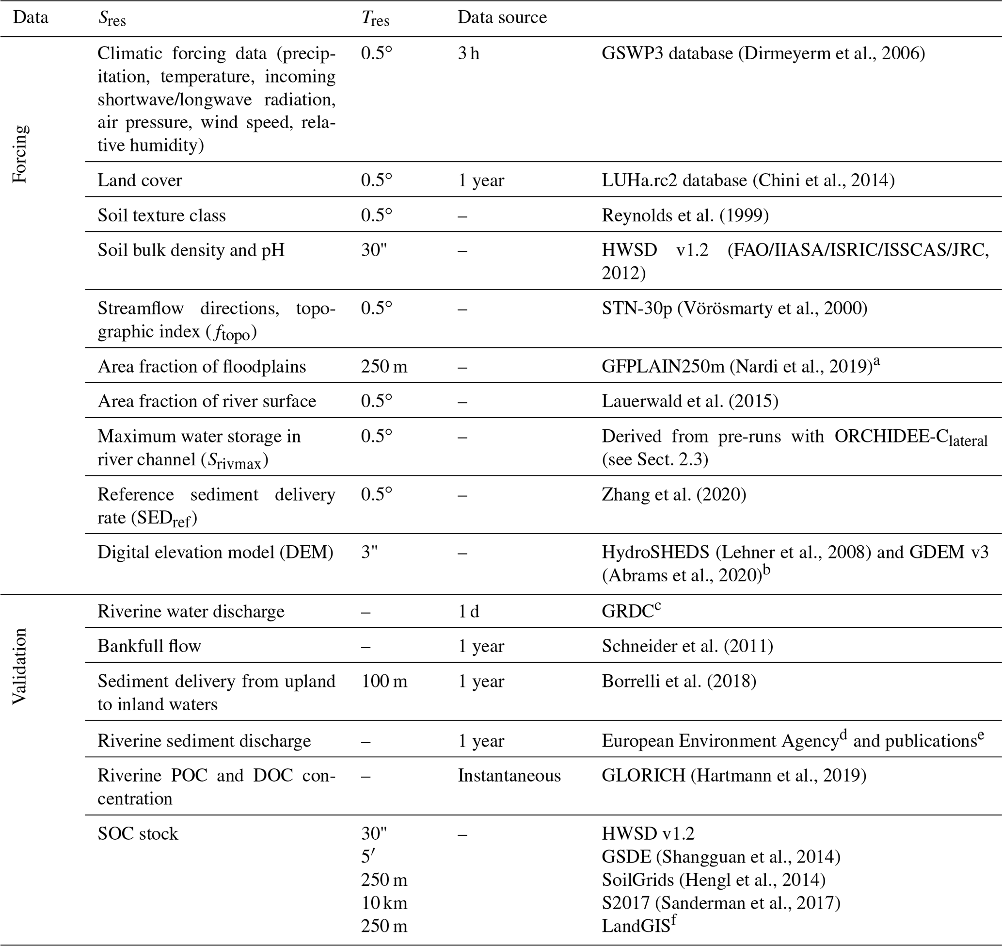
a GFPLAIN250m only covers the regions south of 60∘ N. We produced a map of floodplain distribution in regions north of the 60∘ N using the same method for producing GFPLAIN250m (Nardi et al., 2019) based on the ASTER GDEM v3 database (Abrams et al., 2020). b The DEM data from HydroSHEDS and GDEM v3 are used to extract the topographic properties (e.g., location, area, and average slope) of headwater basins in regions south and north of 60∘ N, respectively.c The Global Runoff Data Centre, 56068 Koblenz, Germany. d https://www.eea.europa.eu/data-and-maps/data/sediment-discharges (last access: 12 May 2020). e Publications including Van Dijk and Kwaad (1998), Vollmer and Goelz (2006), and reports of the DanubeSediment project (Sediment Management Measures for the Danube, http://www.interreg-danube.eu/approved-projects/danubesediment, last access: 24 June 2020). f https://zenodo.org/record/2536040#.YC-QGo9KiUm (last access: 14 October 2020).
Simulation of the lateral transfer of DOC and CO2 in river networks, i.e., the transfer of DOC and CO2 from one basin to another based on the streamflow directions obtained from a forcing file (0.5∘, Table 1), follows the routing scheme of water (Guimberteau et al., 2012). For each basin with a floodplain (defined by forcing data), bankfull flow occurs when stream volume in the river channel exceeds a threshold prescribed by the forcing file (Table 1). DOC and CO2 in flooding waters can enter into soil DOC and CO2 pools along with the flooding water infiltrated into soil. The infiltration rate of flooding water depends on soil properties and soil water content, but it does not depend on vegetation cover. On the contrary, DOC and CO2 originating from the decomposition of submerged litter and SOC in the floodplains is added to the overlying flooding waters. Note that the turnover times of litter and SOC under flooding waters are assumed to be 3 times the litter and SOC turnover times in upland soil (Reddy and Patrick, 1975; Neckles and Neill, 1994; Lauerwald et al., 2017). After removing the infiltrated and evaporated water, the amount of remaining flooding water, as well as the DOC and dissolved CO2 returning to the river channel at the end of each day, is calculated based on a time constant of flooding water (4.0 d, d'Orgeval et al., 2008) modified by a basin-specific topographic index (ftopo, unitless) (Lauerwald et al., 2017).
Decomposition of DOC in stream and flooding waters is calculated at daily time step based on the prescribed turnover times of labile (2 d) and refractory (80 d) DOC in waters (when temperature is 28 ∘C) and a temperature factor obtained from Hanson et al. (2011). CO2 evasion in inland waters is simulated using a much finer integration time step of 6 min. The CO2 partial pressures (pCO2) in the water column are first calculated based on the temperature-dependent solubility of CO2 and the concentration of dissolved CO2 (Telmer and Veizer, 1999). Then the CO2 evasion is calculated based on the gas exchange velocity, the water–air gradient in pCO2, and the surface water area available for gas exchange (Lauerwald et al., 2017). The effect of wind speed on CO2 evasion is not represented in the current version of ORCHILEAK. In addition, swamp and wetland are represented in the routing scheme of ORCHILEAK. More detailed descriptions can be found in Lauerwald et al. (2017).
2.1.2 Sediment and particulate organic carbon delivery from upland soil to river network
To give an accurate simulation of sediment delivery from uplands to the river network and maintain computational efficiency, an upscaling scheme which integrates information from high-resolution (3") topographic and soil erodibility data into a LSM forcing file at 0.5∘ spatial resolution has been introduced (see details in Zhang et al., 2020, Fig. 1). With this upscaling scheme, the erosion-induced sediment and POC delivery from upland soils to the river network, as well as the changes in SOC profiles due to soil erosion, had already been implemented in ORCHIDEE-MUSLE (Zhang et al., 2020). The sediment delivery from small headwater basins (which are basins without perennial streams and are extracted from high-resolution, e.g., 3", digital elevation model – DEM – data; Fig. 1a, d) to the river network (i.e., gross upland soil erosion – sediment deposition within headwater basins) is simulated using the Modified Universal Soil Loss Equation model (MUSLE, Williams, 1975). As introduced in Zhang et al. (2020), “the daily sediment delivery rate from each headwater basin (Si_ref, Mg d−1 basin−1) is first calculated for a given set of reference runoff and vegetation cover conditions (Fig. 1e):
where Qi_ref is the total water discharge (m3 d−1) at the outlet of headwater basin i for the daily reference runoff condition (Rref) of 10 mm d−1 (see Table S1 for the definitions of all abbreviations used in this study). In Eq. (1), qi_ref is the daily peak flow rate (m3 s−1) at the headwater basin outlet under the assumed reference runoff condition. Similar to the SWAT model (Soil and Water Assessment Tool, Neitsch et al., 2011), qi_ref was calculated from the reference maximum 30 min runoff (1 mm 30 min−1) depth and drainage area (DAi, m2) according to the following equation:
where R30_ref (=1 mm 30 min−1) is the assumed daily maximum 30 min runoff”. The coefficients a and b in Eq. (1) and c and d in Eq. (2) need to be calibrated (see Sect. 2.3 and Table 2). In Eq. (1), the term LSi is the combined dimensionless slope length and steepness factor calculated based on the DAi and the average slope steepness (extracted from a DEM) of headwater basin i (Moore and Wilson, 1992). Cref (0–1, dimensionless) in Eq. (1) represents the cover management factor, which depends on vegetation cover and storage of plant debris (see below). The value of Cref is set to 0.1 for the reference state. The soil erodibility factor Ki (Mg MJ−1 mm−1) is calculated using the method of the EPIC model (Sharpley and Williams, 1990) based on SOC and soil texture data obtained from the GSDE database (Table 1). The term Pref (0–1, dimensionless) in Eq. (1) is a factor representing erosion control practices. It was set to 1, as we did not consider the impacts of soil conservation practices in reducing soil erosion rate. Note that it does not matter which value is chosen for Rref, R30_ref, and Cref as long as they are used consistently throughout a study.
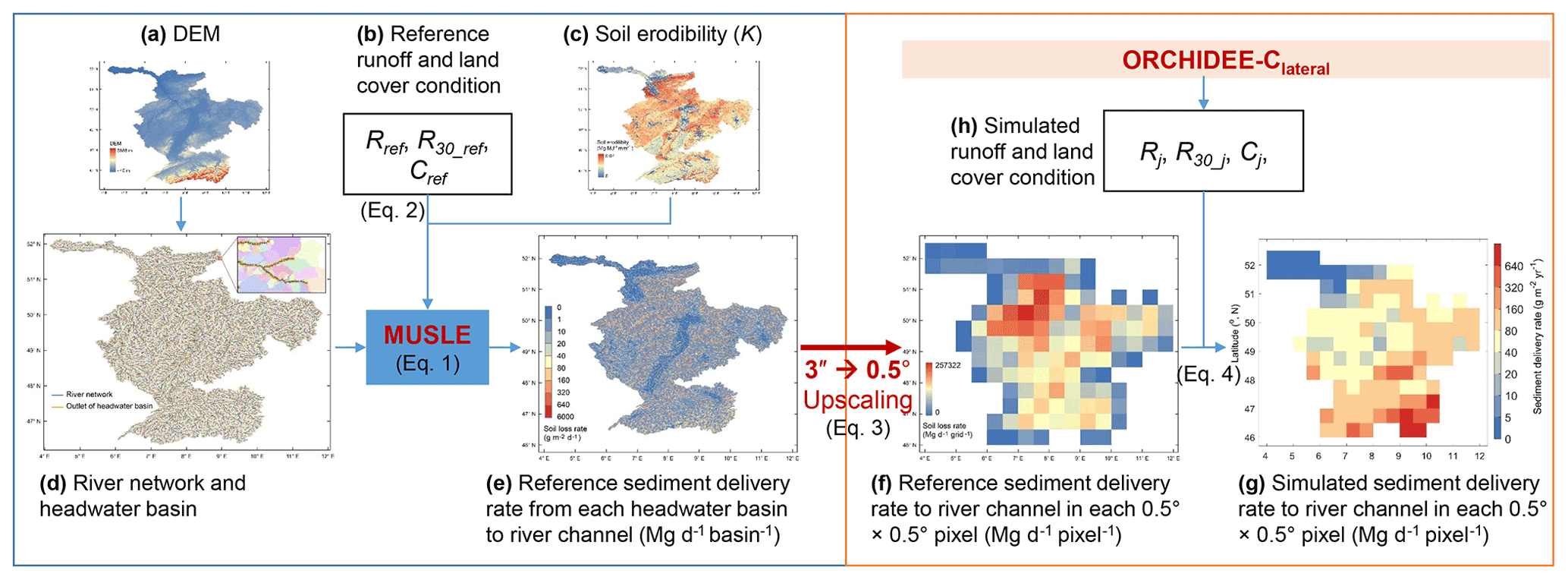
Figure 1Upscaling scheme used in ORCHIDEE-MUSLE (Zhang et al., 2020) and ORCHIDEE-Clateral for calculating the sediment delivery rate from headwater basins to river networks. MUSLE is the Modified Universal Soil Loss Equation; DEM is the digital elevation model (m); K is the soil erodibility factor (Mg MJ−1 mm−1); Rref is the assumed reference daily runoff depth (10 mm d−1); R30_ref is the assumed reference maximum 30 min runoff depth (1 mm 30 min−1); Cref (0.1, dimensionless) is the assumed reference cover management factor; Riday, R30_iday, and Ciday are the simulated daily total runoff depth, daily maximum 30 min runoff depth, and daily cover management factor, respectively. This figure is adapted from Fig. 1 in Zhang et al. (2020).
Table 2Values of the key parameters used in ORCHIDEE-Clateral to simulate the lateral transfer of sediment and carbon.
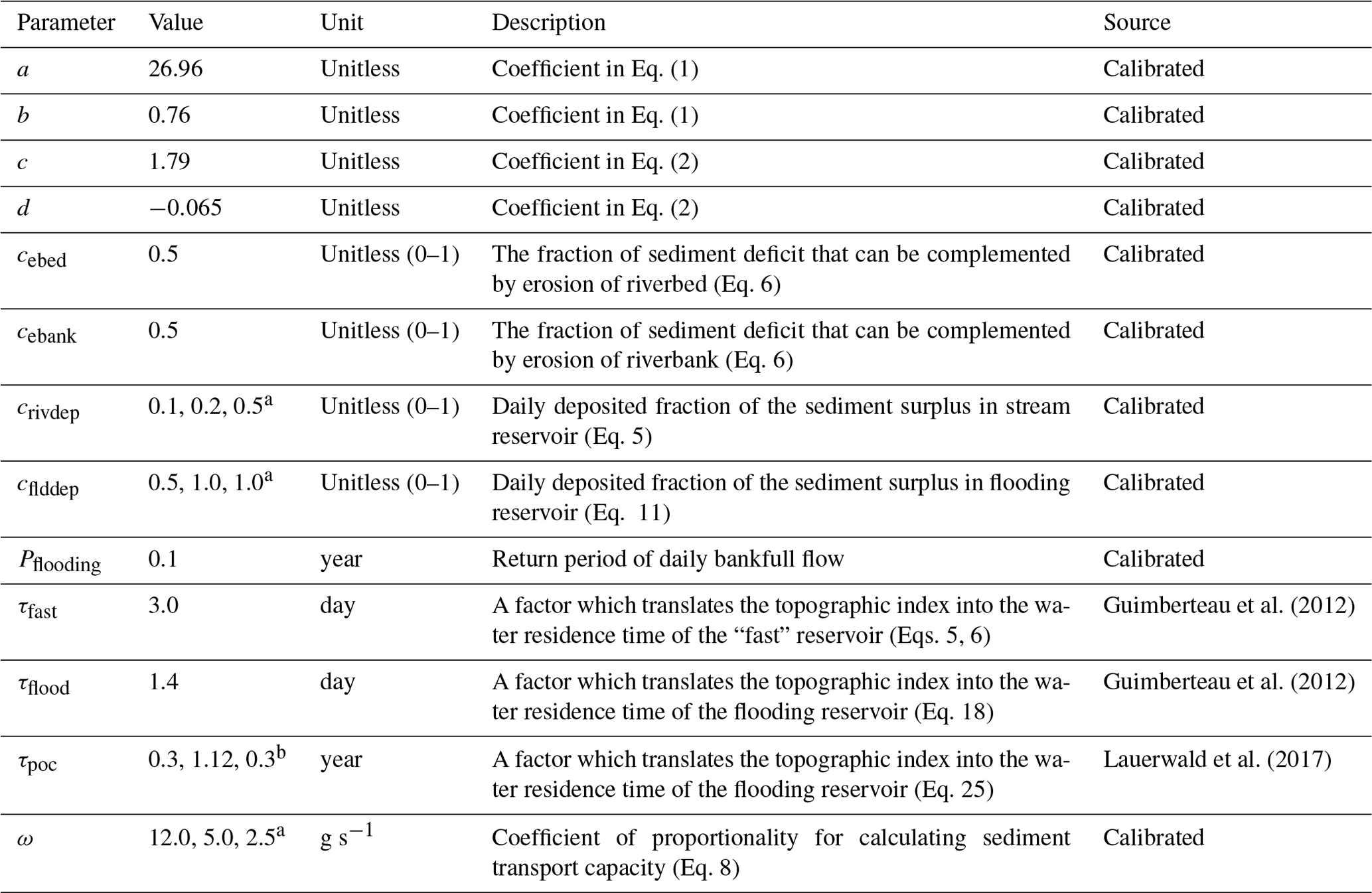
a For clay, silt, and sand sediment, respectively. b For active, slow, and passive POC, respectively.
For the use of these reference sediment delivery estimates in ORCHIDEE-Clateral, the values were first calculated for each headwater basin derived from high-resolution geodata (Fig. 1e), then aggregated to 0.5∘ grid cells (Fig. 1f) – the scale used in our simulations and required to maintain computational efficiency (also limited by the availability of climate and land cover forcing data).
This aggregated dataset is then used to force the simulation of the actual daily sediment delivery (Sj, g d−1 grid−1) in ORCHIDEE-Clateral, simply based on the estimated reference sediment delivery rates of Eq. (1) and on the ratios between actual runoff and land cover conditions as well as the assumed reference conditions used to create that forcing file (Eq. 4, Fig. 1g):
where Rj (mm d−1) is the total surface runoff on day j simulated by the hydrological module or ORCHIDEE-MUSLE at 0.5∘ spatial resolution every 30 min. R30_j (mm 30 min−1) is the maximum value of the 48 half-hour runoffs in each day. Cj (0–1, unitless) is the daily actual cover management factor calculated based on the fraction of surface vegetation cover, the amount of litter stock, and the biomass of living roots in each PFT within each grid cell. Rref, R30_ref, Cref, and Pref are the reference values used to estimate the reference sediment delivery rates as describe above.
Daily POC delivery to the river headstream in each 0.5∘ grid cell is finally simulated based on the sediment delivery rate and the average SOC concentration of surface soil layers (0–20 cm). We assumed that litter cannot be eroded and transported to the river network; however, it can affect the soil erosion rate through the cover management factor of the MUSLE model (denoted by Cj, Eq. 4). The vertical SOC profile is updated every day based on the average depth of eroded soil for each PFT in each 0.5∘ grid cell of ORCHIDEE. For a more detailed description of ORCHIDEE-MUSLE, we refer to Zhang et al. (2020).
2.2 Sediment and POC transport in inland water network
By merging the model branches ORCHILEAK and ORCHIDEE-MUSLE, the new branch ORCHIDEE-Clateral combines the novel features of both sources (DOC and POC) described above. The development of ORCHIDEE-Clateral is complemented by a representation of the sediment and POC transport through the river network that is completely novel and described below.
2.2.1 Sediment transport
Simulation of sediment transport through the river network basically follows the routing scheme of surface water and DOC of ORCHILEAK (Fig. 2). Along with surface runoff (FRO_h2o, m3 d−1), the sediment delivery (FRO_sed, g d−1) from uplands in each basin (i.e., each 0.5∘ grid cell in the case of this study) initially feeds an aboveground water reservoir (Sfast_h2o, m3) with a so-called fast water residence time. From this fast water reservoir, a delayed outflow feeds into the so-called stream reservoir (Sriv, m3, Fig. 2b). Daily water (FFout_h2o, m3 d−1) and sediment (FFout_sed, g d−1) flows from the fast water reservoir to the stream reservoir are calculated from a grid-cell-specific topographic index ftopo (unitless, Vörösmarty et al., 2000) extracted from a forcing file (Table 1) and a reservoir-specific factor τ, which translates ftopo into a water residence time of each reservoir (Eqs. 5, 6). Following Guimberteau et al. (2012), the τ of the fast water reservoir (τfast) is set to 3.0 d. As the sediment delivery calculated from MUSLE is the net soil loss from headwater basins (gross soil erosion – soil deposition within headwater basins), we assumed that there is no sediment deposition in the fast reservoir and that all of the sediment in the fast reservoir enters the stream reservoir. In addition, only the surface runoff causes soil erosion. The belowground drainage (FDR_h2o, m3 d−1) only transports DOC and dissolved CO2 to the stream reservoir (Fig. 2b).
The budget of the suspended sediment in the stream (Sriv_sed, g) is determined by Fout_sed, the upstream sediment input (Fup2riv_sed, g d−1), the sediment input by flooding water returning to the river (Ffld2riv_sed, g d−1), the re-detachment of the previously deposited sediment in the riverbed (Frero_sed, g d−1), the bank erosion (Fbero_sed, g d−1), the sediment deposition in the riverbed (Frd_sed, g d−1), and the sediment transported to downstream river stretches (Fdown2riv_sed, g d−1) and, occasionally, floodplains (Friv2fld_sed, g d−1) (Eq. 7).
Sediment transport capacity (TC, g m −3) is defined as the maximum concentration of suspended sediment that a given flow rate can carry. TC and the flow rate determine the amount of sediment that can be transported to the downstream grid cell (e.g., Fdown2riv_sed, Friv2fld_sed). Suspended sediment loads that are in excess of the maximum possible amount of transported sediment will deposit on the riverbed (Frd_sed). If sediment loads are below that maximum possible amount, erosion of the riverbed (Frero_sed) or riverbank (Fbero_sed) takes place (Arnold et al., 1995; Nearing et al., 1989; Neitsch et al., 2011).
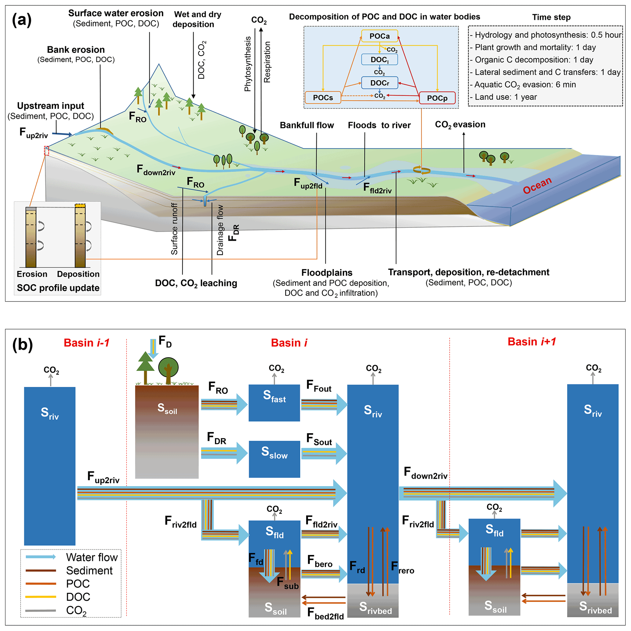
Figure 2Simulated lateral transfer processes of water, sediment, and carbon (POC, DOC, and CO2) in ORCHIDEE-Clateral (a) and a schematic plot for the reservoirs and flows of water, sediment, and carbon represented in the routing module of ORCHIDEE-Clateral (b). Ssoil is the soil pool. Srivbed is the sediment (also POC) deposited on the riverbed. Sfast, Sslow, Sriv, and Sfld are the “fast”, “slow”, stream, and flooding water reservoir, respectively. FRO and FDR are the surface runoff and belowground drainage, respectively. FFout and FSout are the flows from the fast and slow reservoir to the stream reservoir, respectively. Fup2riv and Fdown2riv are the upstream inputs and downstream outputs, respectively. Friv2fld is the output from the river stream to the flooding reservoir. Ffld2riv is the return flow from the flooding reservoir to the stream reservoir. Fbed2fld is the transformation from deposited sediment in a riverbed to floodplain soil. Fbero is bank erosion. Frd and Frero are the deposition and re-detachment of sediment and POC in a river channel, respectively. Fsub is the flux of DOC and CO2 from floodplain soil (originating from the decomposition of submerged litter and soil carbon) to the overlying flooding water. Ffd is the deposition of sediment and POC as well as the infiltration of water and DOC. FD is the wet and dry deposition of DOC from the atmosphere and plant canopy. DOCl and DOCr are the labile and refractory DOC pool, respectively. POCa, POCs, and POCp are the active, slow, and passive POC pool, respectively.
In this study, we used an empirical equation adapted from the WBMsed model, which has been proven effective in simulating the suspended sediment discharges in global large rivers (Cohen et al., 2014), to estimate the TC of suspended sediment concentration in streamflow (g m−3):
where ω is the coefficient of proportionality, qave (m3 s−1) is the long-term average streamflow rate obtained from a historical simulation by ORCHILEAK (Table 1), qj (m3 s−1) is streamflow rate on day j, e1 is an exponent depending on the upstream drainage area (DA, m2), and Fdown2riv_h20 (m3 d−1) is the daily downstream water discharge from the stream reservoir. In the stream reservoir of each basin, net deposition occurs when TC is smaller than the concentration of suspended sediment, and the daily deposited sediment (Frd_sed, g d−1) is calculated based on the surplus of the suspended sediment:
where crivdep (0–1, unitless) is the daily deposited fraction of the sediment surplus. Net erosion of the previously deposited sediment in the riverbed (Srivbed_sed, Fig. 2) or riverbank occurs when TC is larger than the concentration of suspended sediment. We assumed that the erosion of the riverbank occurs only after all of the Srivbed_sed has been eroded. Thus, the daily erosion rate (Frero_sed, g d−1) in a river channel is calculated as
where cebed (0–1, unitless) and cebank (0–1, unitless) are the fraction of sediment deficit that can be complemented by erosion of the riverbed and riverbank, respectively. After updating the Sriv_sed based on the Frd_sed or Frero_sed, the sediment discharge to the downstream basin (Fdown2riv_sed, g d−1) is calculated based on the ratio of downstream water discharge to the total stream reservoir.
In each basin, the bankfull flow occurs when Sriv_h2o exceeds the maximum water storage of the river channel (Srivmax, g), which is defined by a forcing file (Table 1). Sediment flow from the stream to the floodplain (Friv2fld_sed, g d−1) follows the flooding water, and it is calculated as
where fA_fld (0–1, unitless) and fA_riv (0–1, unitless) represent the fraction of floodplain area and river surface area in each basin, respectively. Following the routing scheme of ORCHILEAK, the bankfull flow of a specific basin is assumed to enter the floodplain in the neighboring downstream basin instead of the basin where it originates.
The sediment balance in a flooding reservoir (Sfld_sed, g) is controlled by sediment input from the upstream basins (Friv2fld_sed, g d−1), the sediment flowing back to the stream reservoir (Ffld2riv_sed, g d−1), and the sediment deposition (Ffd_sed, g d−1) (Fig. 2).
Sediment deposition in a floodplain is calculated as the sum of a natural deposition and the deposition due to evaporation (Eh2o, m3 d−1) and infiltration (Ih2o, m3 d−1) of the flooding waters:
where cflddep (0–1, unitless) is the daily deposited fraction of the suspended sediment in flooding waters. After removing the deposited sediment from Sfld_sed, Ffld2riv_sed is calculated based on the ratio of ratio of Ffld2riv_h2o to the total flooding reservoir:
where τflood is a factor which translates ftopo (Table 1) into a water residence time of the flooding reservoir. The same as ORCHILEAK, it is set to 1.4 (d m−2) in this study.
Note that as the upland soil in ORCHIDEE is composed of clay, silt, and sand particles, the dynamics of clay, silt, and sand sediment in inland waters are simulated separately. To represent the selective transport of clay, silt, and sand sediment, the model parameters ω (Eq. 8) and crivdep (Eq. 10) are set to different values when calculating the sediment transport capacity and the deposition of surplus suspended sediment for different particle sizes (Table 2). Moreover, as our model mainly aims to simulate the lateral transfer of sediment and carbon at the decadal to centennial timescale, rather than covering the past thousands of years or even longer time periods, we did not consider the evolution and diversion of river channels in our study.
2.2.2 POC transport and decomposition
Many studies described the selective transport of POC and sediment of different particle sizes. The enrichment ratio (defined as the ratios of the fraction of any given component in the transported sediment to that in the eroded soils) of POC in the transported sediment generally showed significant positive correlation with the fine sediment particles (e.g., fine silt and clay) but negative correlation with the coarse sediment particles (Galy et al., 2008; Haregeweyn et al., 2008; Nadeu et al., 2011; Nie et al., 2015). In ORCHIDEE-Clateral, the physical movements of POC in inland water systems are simply assumed to follow the flows of the finest clay sediment (Fig. 2b). For example, the fractions of riverine suspended POC, which is deposited on the riverbed (Frd_POC, g C d−1) or transported to the river channel (Fdown2riv_POC, g C d−1) or floodplain (Friv2fld_POC, g C d−1), are assumed to be equal to the corresponding fractions of clay sediment (Eqs. 19–21). Also, flows of suspended POC in flooding waters to floodplain soil (Ffd_POC, g C d−1) or back to the stream reservoir (Ffld2riv_POC, g C d−1), as well as the resuspension of POC from the riverbed (Frero_POC, g C d−1), are scaled to the simulated flows of clay sediment (Eqs. 22–24). Note that, similar to SOC, the POC in aquatic reservoirs is divided into three pools: the active (POCa), slow (POCs), and passive pool (POCp) (Fig. 2a). The eroded active, slow, and passive SOC flows into the corresponding POC pools in the “fast” water reservoir (Fig. 2b).
The representation of POC deposition and transformation in the aquatic reservoirs and bed sediment also involves decomposition, which largely follows the scheme used for SOC (Fig. 2a). However, instead of using the rate modifiers for soil temperature and moisture used in the soil carbon module, daily decomposition rates (FPOC_i, g C d−1) of each POC pool (SPOC_i, g C) are simulated to vary with water temperature based on the Arrhenius term, which is used to simulate the DOC decomposition in ORCHILEAK (Hanson et al., 2011; Lauerwald et al., 2017):
where Twater (∘C) is the temperature of water reservoirs and is calculated from local soil temperature using an empirical function (Lauerwald et al., 2017). For the POC stored in bed sediment, the temperature of the stream reservoir is used to calculate the decomposition rate. τPOC_i is the turnover time of the i (active, slow, and passive) POC pool. We assumed that the base turnover times of active (0.3 year) and slow (1.12 years) POC pools are the same as for the corresponding SOC pools. The passive SOC pool is generally regarded as the SOC associated with soil minerals or enclosed in soil aggregates (Parton et al., 1987). During the soil erosion and sediment transport processes, the aggregates break down and the passive POC loses its physical protection from decomposition (Chaplot et al., 2005; Z. Wang et al., 2014; Polyakov and Lal, 2008; X. Wang et al., 2014). To represent the acceleration of passive POC decomposition due to aggregate breakdown, we assume that the turnover time of the passive POC is the same as the active POC (0.3 year) rather than the passive SOC (462 years). Similar to the scheme used to simulate SOC decomposition in ORCHILEAK, the decomposed POC from the active, slow, and passive pools flows to other POC pools, flows to DOC pools, or is released to the atmosphere as CO2 (Fig. 2). Fractions of the decomposed POC flowing to different POC and DOC pools or to the atmosphere are set to the same values used in ORCHILEAK for simulating the fates of the decomposed SOC pools.
Changes in the vertical SOC profile of floodplain soils following sediment deposition are simulated at the end of every daily modeling time step, after physical transfers and decomposition of POC have been calculated. The sediment deposited on the floodplain becomes part of the surface soil layer, and the active, slow, and passive POC flows into the active, slow, and passive SOC pools in surface soil layer, respectively. SOC in the original surface and subsurface soil layers is sequentially transferred to the adjacent deeper soil layers. As the vertical soil profile in ORCHILEAK is described by an 11-layer discretization of a 2 m soil column, we introduce a deep (>2 m) soil pool (Sdeep) to represent the soil and carbon transferred down from the 11th soil layer following ongoing floodplain deposition. Decomposition rates of the organic carbon in this deep soil pool are assumed to be the same as those in the 11th (deepest) soil layer. Note that when the soil erosion rate of the floodplain soil is larger than the sediment deposition rate, sediment and organic carbon in Sdeep move up to replenish the stocks of the 11th soil layer.
2.3 Model application and evaluation
In this study, ORCHIDEE-Clateral was applied over Europe and parts of the Middle East (−30∘ W–70∘ E, 34–75∘ N), where extensive observation datasets are available to calibrate and evaluate our model (Table 1). The return period of daily bankfull flow (Pflooding, year), which represents the average interval between two flooding events, is used in this study to produce the forcing file of Srivmax from a pre-run of ORCHILEAK. Note that Pfloodingis generally shorter than the return period of real flooding events, as the flooding may occur on several continuous days and all the flooding waters occurring on these continuous days are generally regarded as belonging to the same flooding event (Fig. S2 in the Supplement). To our knowledge, existing observational data on Pflooding are still very limited. Therefore, following Schneider et al. (2011), we also use a constant Pflooding to simulate the bankfull flows from European rivers and the observed long-term (1961–2000) average bankfull flow rate (m3 s−1) at 66 sites obtained from Schneider et al. (2011) to calibrate Pflooding (the optimized value is 0.1 year, Table 2). To our knowledge, there are still no large-scale observation data on the sediment delivery rates from land to river networks in Europe. Therefore, following Zhang et al. (2020), the parameters a, b, c, and d in Eqs. (1) and (2) (Table 2) were calibrated for 57 European catchments (Fig. S3d) against the modeled sediment delivery data obtained from the European Soil Data Centre (ESDAC, Borrelli et al., 2018). The sediment delivery data from the ESDAC product were derived from WaTEM/SEDEM model simulations using high-resolution data for topography, soil erodibility, land cover, and rainfall. This model was calibrated and validated using observed sediment fluxes from 24 European catchments (Borrelli et al., 2018).
Parameters controlling sediment transport, deposition, and re-detachment (i.e., ω, crivdep, cflddep, cebed, and cebank, Table 2) in stream and flooding reservoirs were calibrated against the observed long-term averaged sediment discharge rate (Table 1). We also conducted an analysis to test the sensitivity of the simulated riverine sediment and carbon discharges to these parameters following the method used in Tian et al. (2015). The sensitivity of simulation results was evaluated based on the relative changes in simulated riverine sediment and carbon discharges to a 10 % increase and decrease in each parameter (Table 2). The result of the sensitivity analysis shows that the simulated riverine sediment and POC discharges are most sensitive to crivdep in Eq. (10), followed by ω in Eq. (8) (Fig. S4). Compared to crivdep and ω, the simulated riverine sediment and POC discharges are less sensitive to cflddep, cebed, and cebank. With 10 % changes in cflddep, cebed, or cebank, the changes in riverine sediment and POC discharges are generally less than 3 %. In addition, the changes in simulated riverine DOC and CO2 discharges are mostly less than 1 % with 10 % changes in ω, cflddep, cebed, and cebank. Nonetheless, a 10 % change in crivdep can lead to a change of about 5 % in the simulated riverine CO2 discharge (Fig. S4).
After parameter calibration, ORCHIDEE-Clateral was applied to simulate the lateral transfers of water, sediment. and organic carbon in European rivers over the period 1901–2014. Before this historical simulation, ORCHIDEE-Clateral was run over 10 000 years (spin-up) until the soil carbon pools reached a steady state. In the “spin-up” simulation, the PFT maps, atmospheric CO2 concentrations, and meteorological data during 1901–1910 were used repeatedly as forcing data. The final simulated water discharge rates in European rivers were evaluated using observation data at 93 gauging sites (locations see Fig. S3a) from the Global Runoff Database (GRDC, Table 1). The simulated bankfull flows were evaluated against observed long-term (1961–2000) average bankfull flows at 66 sites (Fig. S3b) from Schneider et al. (2011). The simulated riverine sediment discharge rate is evaluated using observation data from the European Environment Agency and existing publications (see Table 1) at 221 gauging sites (Fig. S3c). The riverine total organic carbon (TOC), POC, and DOC concentrations provided by the GLObal RIver Chemistry Database (GLORICH, Hartmann et al., 2019) at 346 sites (Fig. S3d) were used to evaluate the simulated riverine POC and DOC concentrations. Note that observations in the GLORICH database, which are measured at gauging sites with drainage area <1.0×10⁴ km2, were excluded from our model evaluation because these small catchments cannot be represented by the coarse river network scheme at 0.5∘ (ca. 55 km at the Equator). Among the retained 346 gauging sites, TOC concentrations were measured at 188 sites, and DOC was measured at 314 sites. POC was measured at only two sites (Bad Honnef with 51 measurements and Bimmen with 78 measurements) in the Rhine catchment and one site (Rheine, 36 measurements) in the Ems catchment (Fig. S3d).
3.1 Model evaluation
3.1.1 Stream water discharge and bankfull flow
Evaluation of our simulation results using in situ observation data from Europe rivers indicates that ORCHIDEE-Clateral reproduces the magnitude and interannual variation of water discharge rates well in major European rivers (Figs. 3a and S5). Overall, the simulated riverine water discharge rate explained 94 % (Fig. 3a) of the spatial variation of the observed long-term average water discharge rates across 93 gauging sites in Europe (Fig. S3a). Relative biases (calculated as %, as used through the paper if not otherwise stated) of the simulated average water discharge rates compared to the observations are mostly smaller than 30 % (Fig. 3a). For major European rivers, such as the Rhine, Danube, Elbe, Rhone, and Volga, ORCHIDEE-Clateral also captures the interannual variation of the water discharge rate (Fig. S5). We recognize that ORCHIDEE-Clateral may overestimate or underestimate the water discharge rate in some rivers (Fig. 3a), particularly in smaller rivers where discrepancy between the stream routing scheme (delineation of catchment boundaries) extracted from the forcing data at 0.5∘ resolution and the real river network (Fig. S6) can be substantial. An overestimation or underestimation of the catchment area by the forcing data as respectively found for the Elbe and Rhine will introduce a proportional bias in the average amount of simulated discharge from these catchments. Another problem are stream channel bifurcations, which occur in reality but are not represented in a stream network derived from a digital elevation model. For example, in the Danube river delta, a fraction of the discharge is actually exported to the sea through the Saint George Branch, in addition to the water discharge through the main river channel (Fig. S6b). This explains why the simulated water discharge rate at the outlet of the Danube catchment is larger than the observation at the Ceatal gauging station, Romania (identification number in the GRDC database is 6742900, Fig. S5m), where only the main stream discharge was measured.
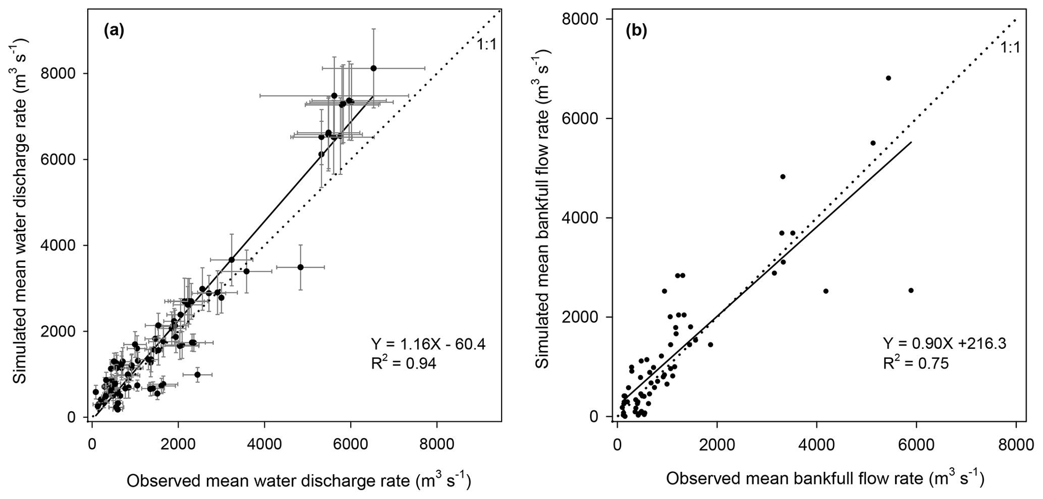
Figure 3Comparison between observed and simulated riverine water discharge rates (a) and bankfull flow rates (b). In panel (a), the error bar denotes the standard deviation of interannual variation. Sources of the observed riverine water discharge rate and bankfull flow rate can be found in Table 1.
With the calibrated return period (0.1 year) of the daily flooding rate (see Sect. 2.3), the simulated bankfull flow rates compare well to observations at the 66 sites for which data were available (Fig. 3b). Overall, the simulation result explained 75 % of the inter-site variation of the observed bankfull flow rates. Relative biases of the simulated bankfull flow rates are generally lower than 30 %, although the relative bias may be larger than 100 % at some sites.
3.1.2 Sediment transport
The simulated area-averaged sediment delivery rates from upland to the river network by ORCHIDEE-Clateral are overall comparable to those simulated by WaTEM/SEDEM for most catchments in Europe (Figs. 4a and S3d). In the two catchments in the Apennine Peninsula, ORCHIDEE-Clateral gives a drastically lower estimation of the sediment delivery rates compared to WaTEM/SEDEM. By excluding these two catchments, ORCHIDEE-Clateral reproduces 72 % of the spatial variation of the sediment delivery rates estimated by WaTEM/SEDEM (Fig. 4a). In addition, the average sediment loss rate over all catchments shown in Fig. S3d is 40.8 g m−2 yr−1, which is overall comparable to the estimate by WaTEM/SEDEM (42.5 g m−2 yr−1).
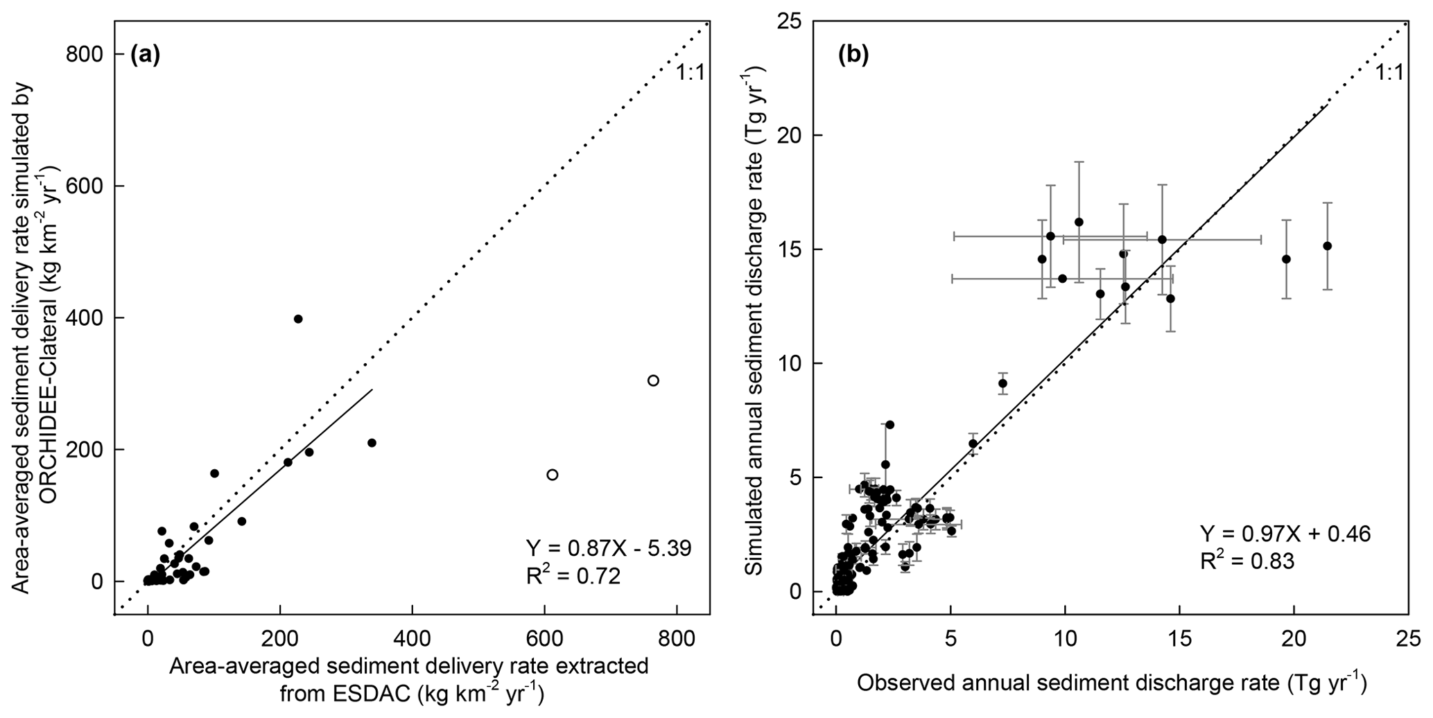
Figure 4Comparison between the simulated area-averaged sediment delivery rate from uplands to the river network from ORCHIDEE-Clateral and WaTEM/SEDEM (a), as well as the comparison between observed and simulated annual sediment discharge rates at 221 gauging sites (b). In panel (a), the two hollow dots represent the sediment delivery rates at the two catchments in the Apennine Peninsula (Fig. S3d). The regression function in panel (a) was obtained based on the values of all solid dots, excluding the two hollow dots. In panel (b), the error bar denotes the standard deviation of interannual variation. Sources of the observed annual sediment discharge rate are in Table 1.
ORCHIDEE-Clateral reproduces 83 % of the inter-site variation of the observed riverine sediment discharge rates across Europe (Fig. 4b). Simulation of the riverine sediment discharge rate at large spatial scale is still a big challenge. It generally needs detailed information on the streamflow, geomorphic properties of river channel, and the particle composition of the suspended sediment (Neitsch et al., 2011). Moreover, the parameters of existing sediment transport models usually require recalibration when they are applied to different catchments (Gassman et al., 2014; Oeurng et al., 2011; Vigiak et al., 2017). In ORCHIDEE-Clateral, the sediment processes in river networks are simulated using simple empirical functions and parameters based on a routing scheme at a spatial resolution of 0.5∘ (Sect. 2.2.1). Detailed information about the streamflow (e.g., cross-sectional area) and the geomorphic properties of river channels is not represented. Sediment discharge in all catchments was simulated using a universal parameter set. This may explain why ORCHIDEE-Clateral fails to capture the observed sediment discharge rates in some specific catchments, especially those with relatively small drainage areas (e.g., <5×10³ km2).
3.1.3 Organic carbon transport
Simulation of the riverine carbon discharge rate at large spatial scale is an even bigger challenge than simulating sediment discharge, as the riverine carbon discharge is controlled by many factors, such as upland topsoil SOC concentrations, soil erosion rate, the transport and deposition rate of the clay fraction in the river channel and on the floodplain, and the decomposition of POC in transit and in aquatic sediments. As described above, the simulated water discharge rate, bankfull flow, and sediment discharge rate are overall comparable to observations (Figs. 3 and 4). The simulated total SOC stock in the top 0–30 cm soil layer in Europe of 107 Pg C is close to the value extracted from the HWSD database (106 Pg C) but significantly lower than the values extracted from some other databases, such as GSDE (249 Pg C), SoilGrids (202 Pg C), S2017 (148 Pg C) and landGIS (226 Pg C) (Fig. S7a). We noticed that the SOC stocks extracted from these observation-based soil databases show considerable difference (vary from 106 to 249 Pg C), as they have been produced using different clusters of site-level SOC measurements and different interpolation methods to produce global gridded SOC stocks from the site-level measurements (Shangguan et al., 2014; Hengl et al., 2014; Sanderman et al., 2017). Distributions of the simulated SOC stock along the latitude gradients (30–75∘ N) are overall comparable to those extracted from the HWSD and S2017 databases (Fig. S7). But even compared to these two databases, our model still underestimated the SOC stock in southern Europe (30–41∘ N).
Comparison of the simulated concentrations of riverine organic carbon and the observations obtained from the GLORICH database (Hartmann et al., 2019) indicates that our model can basically capture the TOC and DOC concentrations in European rivers (Figs. 5, 6, S8 and S9). The simulation results explain 34 % and 32 % of the inter-site variation of the observed TOC and DOC concentrations, respectively (Fig. 5). For major European rivers, such as the Rhine, Elbe, Danube, Spree, and Weser, the simulated long-term average TOC and DOC concentrations are overall close to the observations (Figs. 6, S8, and S9). But for the Rhone river in southern France, the DOC concentrations have been systematically overestimated by more than 50 % (Figs. 6 and S9m). In addition, both simulated and observed TOC and DOC concentrations show drastic temporal (both seasonal and interannual) variations (Figs. 5, S8 and S9). Our model seems to have overestimated the temporal variation of TOC and especially DOC concentrations (Figs. S8 and S9). Nonetheless, the simulated temporal variations of TOC and DOC discharge rates are overall comparable to the observations (Figs. S10 and S11), as our model can capture the magnitude and temporal variation of riverine water discharge rates well.
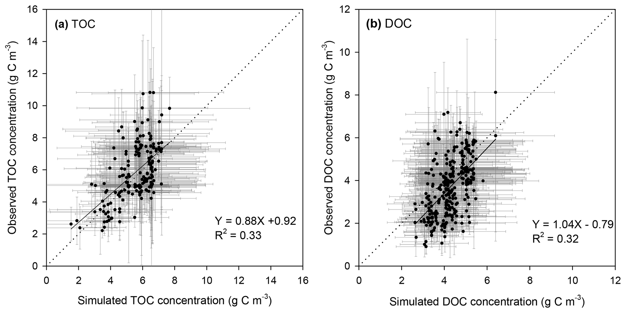
Figure 5Comparison between the observed and simulated riverine TOC (a, POC + DOC) and DOC (b) concentrations. The dot and error bar denote the mean and standard deviation at each gauging site, respectively. Note that the mean and standard deviation of the simulated concentrations at each site are calculated based on the monthly average value, but the mean and standard deviation of the observed concentrations are based on instantaneous observation.

Figure 6Comparison between the observed and simulated concentrations of total organic carbon (TOC, a) and dissolved organic carbon (DOC, b) in river flows, as well as the discharge rates of riverine TOC and DOC. The black and pink lines in each box denote the median and mean value, respectively. Box boundaries show the 25th and 75th percentiles, whiskers denote the 10th and 90th percentiles, and the dots below and above each box denote the 5th and 95th percentiles, respectively.
In Europe, the GLORICH database only provides POC concentrations measured at three gauging stations in northwestern Germany (Figs. 7, S3d). The simulated POC concentrations and discharge rates in the Ems river at Rheine are overall comparable to the observations (Fig. 7e, f). However, at the two gauging sites at the river Rhine, the POC concentrations have been significantly underestimated (Fig. 7a–d). We noticed that the stream routing scheme of the Rhine catchment at 0.5∘ obtained from the forcing data STN-30p (Vörösmarty et al., 2000) differs significantly from the stream routing scheme extracted based on the high-resolution (3") DEM (Fig. S6). Thus, besides the errors in simulated SOC stocks, soil erosion rate, stream discharge rate, and sediment transport and deposition rate, the inaccurate stream routing scheme used in this study might also be an important reason for the underestimation of POC concentration in the Rhine river.

Figure 7Comparison between observed (instantaneous measurements) and simulated (monthly average values) riverine POC concentrations and POC discharge rates at three gauging sites. The histograms and error bars denote the means and standard deviations of POC concentrations, respectively. Long-term average water discharge rates at Bad Honnef, Bimmen and Rheine during the observation periods are 2023, 2100 and 80 m3 s−1, respectively.
3.2 Lateral carbon transfers in Europe
Based on our simulation results, the average annual sediment delivery from upland to the river network caused by water erosion in Europe (−30∘ W–70∘ E, 34–75∘ N) during 1901–2014 is 2.8±0.4 Pg yr−1 (Fig. 8a). From northern to southern Europe, the sediment delivery rate from upland to the river increases from less than 1.0 g m−2 yr−1 in the Scandinavia Peninsula, which is covered by mature boreal forests (Fig. S12a), and in the Northern European Plain to more than 600 g m−2 yr−1 in the mountainous regions of the Apennine Peninsula, Balkan Peninsula, and the Middle East (Figs. 9a, S13a). In total across Europe, 63.2 % (1.8±0.2 Pg yr−1) of the sediment delivered into the river network is deposited in river channels and floodplains, and the remaining 36.8 % (1.0±0.1 Pg yr−1) is exported to the sea (Fig. 8a). Generally, large rivers, like the Danube, Volga, and Ob rivers, carry more sediment to the sea than small rivers (Fig. 9b, c). But several relatively small rivers in the Middle East and the Po river in northern Italy also carry a similarly large amount of sediment to the sea, as the upland soil erosion rates are very high (>200 g m−2 yr−1) in these catchments (Fig. 9a, c). Spatial distribution of the sediment deposition is controlled by the stream routing scheme and the spatial distribution of floodplains (Fig. 10b). In northern and central Europe, the area-averaged sediment deposition rates (i.e., calculated as the amount of annual sediment deposition in each grid cell divided by the grid cell area) in river channels and floodplains are mostly less than 100.0 g m−2 yr−1 (Fig. 9d). In the downstream part of the Danube, Po, and several rivers in the Middle East, the sediment deposition rate can exceed 800.0 g m−2 yr−1. From 1901 to the 1960s, the annual total sediment delivery from uplands to the whole river network of Europe declined significantly (p<0.01, independent sample t test) from about 3.0 Pg yr−1 to about 2.3 Pg yr−1 (Fig. S14a). From 1960 to 2014, the annual sediment delivery rate did not show a significant trend but revealed large interannual variations.

Figure 8Averaged annual lateral redistribution rate of sediment (a), POC (b), DOC (c), and CO2 (d) in Europe for the period 1901–2014. Fsub_DOC and Fsub_CO2 are the DOC and CO2 inputs from floodplain soil (originating from the decomposition of submerged litter and soil carbon) to the overlying flooding water, respectively.
Along with soil erosion and sediment transport, the average annual POC delivery from upland to the river network in the whole of Europe during 1901–2014 is 10.1±1.1 Tg C yr−1 (Fig. 8b). 41.0 % of the POC delivered into the river network is deposited in river channels and floodplains, 2.9 % is decomposed during transport, and the remaining 56.1 % is exported to the sea. Spatial patterns of the area-averaged SOC delivery rate and POC discharge rate basically follow that of sediment (Fig. 10a, c). Although the sediment discharge rates in some rivers in the Middle East can be as high as that in the Danube or Volga river (Fig. 9c), the POC delivery rates in these rivers are much smaller than in the larger ones (Fig. 10c). This is mainly due to the lower SOC stocks in the Middle East compared to those found in the Danube and Volga catchments (Fig. S7). We also note that different from the sediment delivery, the annual total POC delivery from upland to the river network in Europe did not show a significant declining trend from 1901 to the 1960s (Fig. S14b). The increase in SOC stock (Fig. S14c) may have partially offset the decline in sediment delivery rate.

Figure 9Averaged annual lateral redistribution rate of water and sediment in Europe during 1901–2014. (a) Annual sediment delivery rate from upland to the river network; (b) annual water discharge rate; (c) annual sediment discharge rate; (d) annual net sediment budget in each grid cell. In panel (d), the positive and negative values denote net gain and net loss of sediment, respectively.
Leaching results in an average annual DOC input of 13.5±1.5 Tg C yr−1 from soil to the river network in Europe, and the in situ DOC production caused by wet deposition and the decomposition of riverine POC as well as submerged litter and soil organic carbon under flooding waters amounts to 2.2±0.7 Tg C yr−1 (Fig. 8c). 28.1 % of the total riverine DOC then infiltrates the floodplain soils, 12.9 % is decomposed during riverine transport, and the remaining 59.0 % is exported to the sea. The spatial distribution of the DOC leaching rate is very different from that of POC (Fig. 10b). From northwestern Europe to southeastern Europe and the Middle East, the DOC leaching rates decrease from over 6 g C m−2 yr−1 to less than 1.0 g C m−2 yr−1. DOC discharge rates in major European rivers, such as the Rhine, Danube, Volga, Elbe, and Ob, are mostly higher than 100 Tg C yr−1 (Fig. 10d). Comparatively, the DOC discharge rates in southern Europe and the Middle East are significantly lower (<60 Tg C yr−1).

Figure 10Averaged annual lateral redistribution rate of organic carbon in Europe during 1901–2014. (a) Annual SOC delivery rate from upland to the river network; (b) annual DOC leaching rate; (c) annual POC discharge rate; (d) annual DOC discharge rate.
The average annual leaching rate of CO2 sourced from the decomposition of upland litter and soil organic carbon (incl. DOC) in the whole of Europe is 14.3±2.2 Tg C yr−1 (Fig. 8a). Decomposition of the submerged litter and organic carbon in floodplains and the decomposition of riverine POC and DOC add an in situ CO2 production amounting to 7.5±2.7 and 4.1±0.5 Tg C yr−1, respectively. Most of this CO2 (80.2 %) feeding stream waters is then released back to the atmosphere quickly, in such a way that only 15.8 % of the CO2 is exported to the sea, and 4.0 % infiltrates the floodplain soils.
3.3 Implications for the terrestrial C budget of Europe
Representing the lateral carbon transport in an LSM is helpful to estimate the terrestrial carbon cycle more accurately. From the year 1901 to 2014, soil erosion and leaching combined resulted in a 5.4 Pg loss of terrestrial carbon to the European river network, with this amount corresponding to about 5 % of the total SOC stock (106 Pg C, Fig. S7a) in the 0–30 cm soil layer. The average annual total delivery of organic carbon (POC + DOC) during the same period is 47.3±6.6 Tg C yr−1 (Fig. 8), which is about 4.7 % of the net ecosystem production (NEP at 993±255 Tg C yr−1, defined as the difference between the vegetation primary production – NPP – and the soil heterotrophic respiration – Rh – due to the decomposition of litter and soil organic matter, i.e., NEP = NPP − Rh) and 19.2 % of the net biome production (NBP at 243±189 Tg C yr−1, defined as the difference between NEP and the land carbon loss – Rd – due to additional disturbances, e.g., harvest, land cover change, and soil erosion, and leaching, i.e., NBP = NEP − Rd − DOC and POC to the river) (Fig. 11b). The annual total export of carbon to the sea surrounding Europe is 19.0±1.4 Tg C yr−1, which amounts to 1.9 % and 8.7 % of the NEE and NBP, respectively.
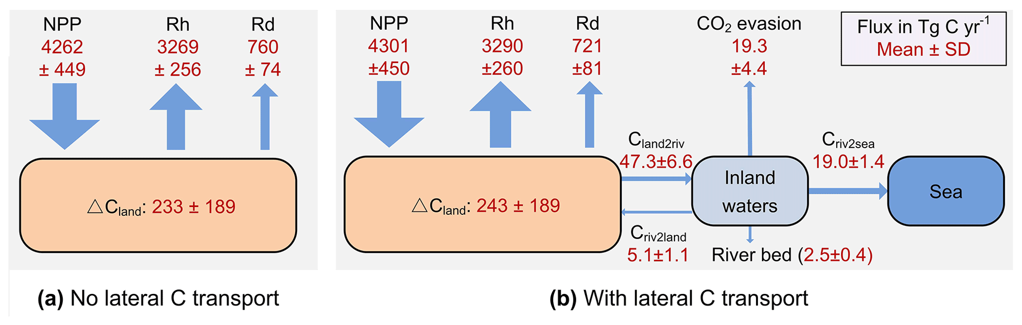
Figure 11The simulated average annual carbon budget of the terrestrial ecosystem in Europe during the 1901–2014 when the lateral carbon transport is ignored (a) and considered (b). All fluxes are presented as mean ± standard deviation. NPP is the net primary production. Rh and Rd are the heterotrophic respiration and the respiration due to disturbances like harvest and land cover change, respectively. ΔCland represents the average annual changes in the total land carbon stock. The percentage following each of these changes in blue represents the average annual relative changes in the corresponding carbon pool. Cland2riv, Criv2land, and Criv2sea are the average annual carbon fluxes from land to inland waters, from inland waters to floodplains, and from inland waters to the sea, respectively. SD is the standard deviation.
Besides direct transfers of organic carbon from soil to aquatic systems, the lateral transport of water, sediment, and carbon can also affect the land carbon budget in several indirect ways. First, the lateral redistribution of surface runoff can affect the land carbon budget by altering soil wetness. Our simulation results reveal that the lateral redistribution of runoff can significantly change local soil wetness, especially in floodplains (Fig. S13b), where the increase in soil wetness can be larger than 10 % (Fig. S16b). Soil wetness is a key controlling factor of plant photosynthesis (Knapp et al., 2001; Stocker et al., 2019; Xu et al., 2013). Benefiting from the increase in soil wetness, the NPP in many grid cells with a large area of floodplain increased by more than 5 % (Fig. 11b), although the NPP over the whole of Europe only increased by 1 % (Fig. 11). Changes in soil wetness can further alter soil temperature (Fig. S16a). As soil wetness and temperature are the two most important controlling factors of organic matter decomposition, the lateral redistribution of runoff can affect the local land carbon budget by changing the Rh. Moreover, in ORCHIDEE-Clateral, the turnover times of litter and SOC under flooding waters (assumed to experience anaerobic conditions) are set to be one-third of the litter and SOC turnover times in upland soil (Reddy and Patrick, 1975; Neckles and Neill, 1994; Lauerwald et al., 2017). Accounting for flooding thus decreases the decomposition rate of litter and SOC stored in floodplain soils.
Second, soil erosion and sediment deposition can affect the land carbon budget by altering the vertical distribution of litter and soil organic carbon. At the net erosion sites of the uplands, the loss of surface soil results in some of the belowground litter and SOC that were originally stored in deeper soil layers emerging to the surface soil layers, and it also results in a fraction of the belowground litter becoming aboveground litter. In the floodplains, the newly deposited sediment becomes part of the surface soil layer, and the belowground litter and SOC in the original surface soil layer are transferred down to the deeper soil layers. As the temperatures and fresh organic matter inputs (sourced from the aboveground litterfall and dead roots), which can impact SOC decomposition rates through the priming effect (Guenet et al., 2010, 2016), in different soil layers are different, changes in the vertical distribution of belowground litter and SOC can therefore lead to changes in the overall decomposition rate of the organic matter in the whole soil column.
Third, soil aggregates mostly break down during soil erosion and sediment transport, and the riverine POC thus loses some of its physically protection from decomposition (Hu and Kuhn, 2016; Lal, 2003). Some modeling studies have assumed that at least 20 % of the eroded SOC would be decomposed during soil erosion and transport processes (Lal, 2003, 2004; Zhang et al., 2014). However, the estimation by Smith et al. (2001) using a conceptual mass balance model suggests that only a tiny fraction of the eroded POC is decomposed and released as CO2 to the atmosphere. Using laboratory rainfall simulation experiments, van Hemelryck et al. (2011) estimated a 2 %–12 % mineralization of the eroded SOC from a loess soil, and X. Wang et al. (2014) estimated a mineralization of only 1.5 %. In ORCHIDEE-Clateral, the passive SOC pool is regarded as the SOC associated with soil minerals and protected by soil aggregates. The turnover time of the passive POC in the river stream and flooding waters is assumed to be the same as that of the active POC (0.3 year). Our simulation results suggest that the fraction of total riverine POC that is decomposed during lateral transport from uplands to the sea is 2.9 % in Europe (Fig. 8b), which is larger than the POC decomposition fraction (0.9 %) when the turnover time of the passive POC in rivers is assumed to be the same as that of the passive POC (i.e., no soil aggregates break down). The acceleration of POC decomposition rate due to the breakdown of soil aggregates can thus slightly affect the estimate of the regional land–atmosphere carbon flux. Moreover, the riverine POC and DOC can be transported over a long distance and finally settle or infiltrate floodplains or river channels (especially estuarine deltas) where the local environmental conditions might be quite different from those encountered in the uplands from where these C pools originate. These changes in environmental conditions can affect the decomposition rate of the laterally redistributed organic carbon (Abril et al., 2002).
Comparison between the simulation results from ORCHIDEE-Clateral with activated and deactivated erosion and river routing modules indicates that ignoring lateral carbon transport processes in LSMs may lead to significant biases in the simulated land carbon budget (Figs. 11 and S14). Although the omission of lateral carbon transport in ORCHIDEE-Clateral only resulted in a 1 % decrease in simulated average annual total NPP in Europe during 1901–2014 and a 1 % increase in annual total Rh, the annual total NBP (NEP–Rd–DOC and POC to the river) is overestimated by 4.5 %. Over the same period, the lateral carbon transport only induced a 0.09 % decrease in the total SOC and DOC stock in Europe (Fig. S15c), but their spatial distribution was significantly altered (Fig. 12e, f). For instance, in some mountainous regions, the soil erosion induced a reduction of the SOC stock by more than 8 %. On the contrary, the sediment and POC deposition in some floodplains led to an increase in SOC stock by more than 8 % (Fig. 12f).
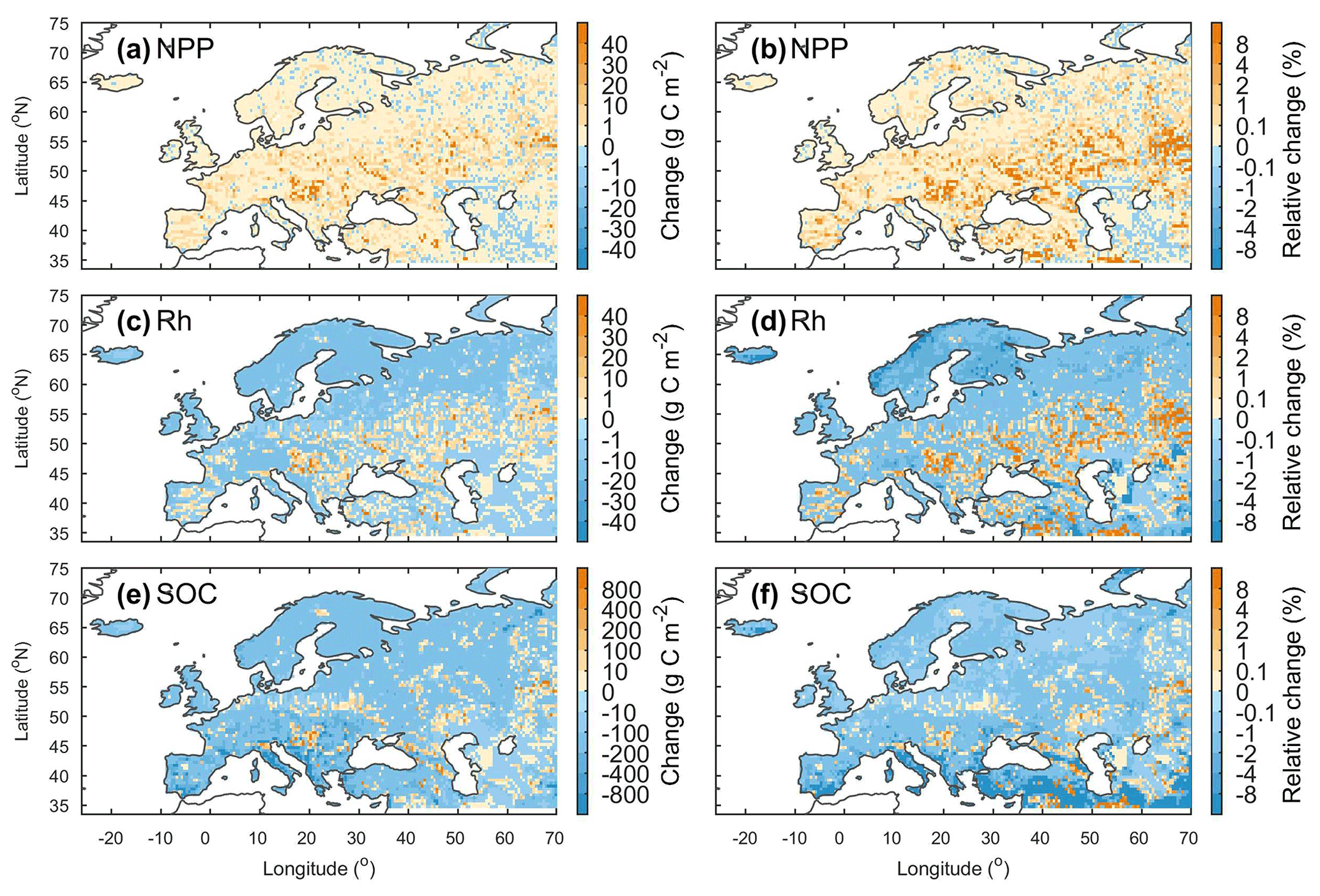
Figure 12Changes (first column) and relative changes (second column) in the net primary production (NPP), heterotrophic respiration (Rh), and total soil organic carbon (SOC, 0–2 m) in Europe due to lateral carbon transport during 1901–2014. For each variable, the change is calculated as Clat−Cnolat, where Clat and Cnolat are the carbon fluxes or stocks when lateral carbon transport is considered and ignored, respectively. The relative changes is calculated as ( %.
Consistent with previous studies (Stallard, 1998; Smith et al., 2001; Hoffmann et al., 2013), our simulation results reveal the importance of sediment deposition in floodplains for the overall SOC budget. From 1901 to 2014, erosion and leaching over Europe totally induced a loss of 3.03 Pg organic carbon (POC + DOC) from uplands to the river network, and only 0.65 Pg of this carbon was redeposited onto the floodplains. The total stock of soil organic carbon in Europe thus should have decreased by 2.38 Pg C. However, due to the decrease in decomposition rate of the buried organic carbon (including in situ and ex situ carbon) in floodplain soils, the total stock of soil organic carbon in Europe only decreased by 0.91 Pg C. Floodplains in Europe have protected a total of 2.12 (= 3.03–0.91) Pg of soil organic carbon from being transported to the sea or released to the atmosphere in forms of CO2. Although the sequestration of organic carbon in floodplains cannot make up all of the soil organic carbon (POC + DOC) loss, the increased organic carbon stock in floodplains (2.12 Pg C) is much higher than the soil POC loss (0.86 Pg C) induced by soil erosion.
3.4 Uncertainties and future work
In the present version of ORCHIDEE-Clateral, the lateral transfers of sediment and carbon are simulated using a simplified scheme due to the fragmented nature of large-scale forcing (e.g., geomorphic properties of the river channel) and validation data (e.g., continuous sediment and carbon concentration data in river streams and deposition–erosion rates in river channels). We recognize that this simplification induces significant uncertainties in model outputs, especially regarding changes in lateral sediment and particulate carbon transfers under climate change and direct human perturbations. Several physics-based algorithms have been proposed to accurately calculate the TC of streamflows (Arnold et al., 1995; Molinas and Wu, 2001; Nearing et al., 1989). These algorithms mostly require detailed information about the stream power (e.g., flow speed and depth), geomorphic properties of the river channel (e.g., slope and hydraulic radius), and the physical properties of the sediment particles (e.g., median grain size) (Neitsch et al., 2011). They are good predictors to estimate TC in rivers with detailed observation data on local stream, soil, and geomorphic properties. Unfortunately, it is not practical to implement those algorithms in ORCHIDEE-Clateral due to the lack of appropriate forcing data at large scale as well as the relatively rough representation of streamflow dynamics compared to hydrological models for small basins. For example, runoff and sediment from all headwater basins in one 0.5∘ grid cell of ORCHIDEE-Clateral are assumed to flow into one single virtual river channel. Although the total river surface area in each grid cell is represented (obtained from forcing file, Table 1, Lauerwald et al., 2015), the length, width, and depth of the river channel are unknown. Furthermore, in reality, there can be multiple river channels in the area represented by each grid cell, and these channels might flow in different directions.
We also noticed that previous studies have derived empirical functions of upstream drainage area (e.g., Luo et al., 2017) or upstream runoff (e.g., Yamazaki et al., 2011) to calculate the river width and depth, allowing simulation of the water flow in the river channel using physically based algorithms. Unfortunately, to obtain a good fit of the simulated river discharges against observations, the parameters in the empirical functions for calculating river width and depth generally need to be calibrated separately for each catchment (Luo et al., 2017), an approach that is incompatible with large-scale simulations like those performed here. Without such calibration, the simulated geometrical properties of the river channel and runoff are prone to large uncertainties, thus rendering the simulation of sediment transport at continental or global scale using physically based algorithms a more challenging task. Given the difficulty of simulating the detailed hydraulic dynamics of streamflow at large spatial scale, we thus apply a simple approach (Eq. 8) to calculate the sediment transport capacity. Overall, we encourage future studies to produce large-scale databases on the geomorphic properties of global river channels (e.g., river depth and width) and to develop large-scale sediment transport models capable of producing more realistic and accurate simulations of sediment deposition, re-detachment, and transport processes, as well as including the exchanges of water, sediment, and carbon between river streams and floodplains.
The simulation of the soil DOC dynamics and leaching in our model needs to be further improved to better simulate the seasonal variation of riverine DOC and TOC concentrations. The concentration of soil DOC and the DOC decomposition rate during the lateral transport process in the river network are the two key factors controlling DOC concentration in river flow. As only a small fraction (<20 %) of the riverine DOC is decomposed during lateral transport (Fig. 8), the overestimated (Fig. 6) seasonal amplitude in riverine DOC (and TOC) concentrations is likely caused by the uncertainties in the simulated seasonal dynamics of the leached soil DOC. The current scheme used in our model for simulating soil DOC dynamics has been calibrated against observed DOC concentrations at several sites in Europe (Camino-Serrano et al., 2018). Although the calibrated model can overall capture the average concentrations of soil DOC, it is not able to fully capture the temporal dynamics of DOC concentrations (Camino-Serrano et al., 2018). Given this, it is necessary to collect additional observation data on the seasonal dynamics of soil DOC concentration to further calibrate the soil DOC model. In addition, averaged over the various DOC and SOC pools we distinguish in the soils, DOC represents a much more reactive fraction of soil carbon (with a turnover time of several days to a few months) than SOC (with a turnover time of decades to thousands of years). Therefore, soil DOC concentrations experience large seasonal variations, while SOC concentrations generally are much more stable and show very limited seasonal dynamics. Overall, seasonal variations in riverine POC concentrations are mainly controlled by the seasonal dynamics of soil erosion rates rather than by the seasonal SOC dynamics, which explains a partial decoupling in the behavior of POC compared to that of DOC.
Although most processes related to lateral carbon transport have been represented in ORCHIDEE-Clateral, there are still omitted processes and large uncertainties in our model. For example, many studies suggest that a substantial portion of the eroded sediment and carbon is deposited downhill at adjacent lowlands as colluviums rather than being exported to the river (Berhe et al., 2007; Smith et al., 2001; Hoffmann et al., 2013; Wang et al., 2010). As the deposition of sediment and carbon within headwater basins can also significantly alter the vertical SOC profile and soil micro-environments (e.g., soil moisture, aeration, and density) (Doetterl et al., 2016; Gregorich et al., 1998; Wang et al., 2015; Zhang et al., 2016), omission of this process may result in uncertainties in the simulated vegetation production and SOC decomposition. In addition, the impact of artificial dams and reservoirs on riverine sediment and carbon fluxes is also not represented in our model. Construction of dams generally leads to increased water residence time, nutrient retention, and sediment and carbon trapping in the impounded reservoir (Habersack et al., 2016; Maavara et al., 2017), and it can also affect the downstream flooding regime and frequency (Mei et al., 2016; Timpe and Kaplan, 2017). Estimation by Maavara et al. (2017) suggests that the organic carbon trapped or mineralized in global artificial reservoirs is about 13 % of the total organic carbon carried by global rivers to the oceans. To more accurately simulate the lateral carbon transport, we plan to include the soil and carbon redistribution within headwater basins and the effects of dams and reservoirs on riverine sediment and carbon fluxes in our model in the near future.
The effects of lateral redistribution of water and sediment on vegetation productivity has not been fully represented in our model. As shown above, our model is able to represent the impacts of lateral water redistribution on vegetation productivity though modifying local soil wetness (Figs. 12 and S16). However, in addition to modifying soil wetness, many studies have indicated that soil erosion and sediment deposition can affect vegetation productivity by modifying soil nutrient (e.g., nitrogen – N and phosphorus – P) availability (Bakker et al., 2004; Borrelli et al., 2018; Quine, 2002; Quinton et al., 2010). Recently, terrestrial N and P cycles have already been incorporated into another branch of ORCHIDEE (i.e., the ORCHIDEE-CNP developed by Goll et al., 2017). By coupling our new branch and ORCHIDEE-CNP, it will be possible to develop a more comprehensive LSM that can also simulate the effects of lateral N and P redistribution on vegetation productivity.
Although soils are the major source of riverine organic carbon, domestic, agricultural, and industrial waste, as well as river-borne phytoplankton, can also make significant contributions (Abril et al., 2002; Meybeck, 1993; Hoffmann et al., 2020). Moreover, previous studies have shown that sewage generally contains highly labile POC, while most aquatic production is generally mineralized within a short time (Abril et al., 2002; Caffrey et al., 1998). Omission of organic carbon inputs from manure and sewage could potentially lead to an underestimation of CO2 evasion from the European river network. Inclusion of these additional carbon sources should thus help improve simulation of aquatic CO2 evasion.
Uncertainties in our simulation results also stem from the forcing data (Table 1) applied in our model. The routing scheme of water, sediment, and carbon is driven by a map of streamflow direction at 0.5∘ spatial resolution (Guimberteau et al., 2012). Comparison between this flow direction map and the flow direction map derived based on a high-resolution (3") DEM shows discrepancies between the two river flow networks (Fig. S6). As the flow direction directly determines the area of each catchment and the route of river flows, errors in forcing data for flow direction may thus induce uncertainties in the simulated riverine water, sediment, and carbon discharges. Land cover maps are another source of uncertainty. For instance, croplands generally experience significantly larger soil erosion rates than grasslands and forests (Borrelli et al., 2017; Nunes et al., 2011; Zhang et al., 2020). However, croplands in ORCHIDEE are only represented in a simplified way by segmenting them into C3 and C4 crops based on their photosynthesis characteristics. Therefore, our simulations based on land cover data with only two broad groups of crops might not be able to fully capture the seasonal dynamics of planting, canopy growth rate, and harvesting for all crop types. Furthermore, the effects of soil conservation practices, which would decrease erosion rates, are ignored in our model. Panagos et al. (2015) have shown that contour farming as well as stone wall and grass margin techniques have been applied in Europe to reduce the risk of soil erosion. However, these soil conservation practices only reduce the average erosion rate in the European Union by 3 %. Excluding soil conservation practices should thus have a limited impact in our simulation results.
Further model calibration, evaluation, and development are necessary for improving our model. Due to the limitation of observation data, we calibrated the parameters controlling sediment transport, deposition, and re-detachment (i.e., ω, crivdep, cflddep, cebed, and cebank in Table S1) in streams and flooding reservoirs only against the observed sediment yield. Even though our model can overall capture the lateral transfers of sediment and carbon in many rivers in central and northern Europe, more observation data are crucially needed to further evaluate the performance of our model, in particular in southern Europe. In addition, it is still unknown whether our model can satisfactorily simulate intermediate processes such as sediment deposition in river channels and floodplains, as well as the rate of river channel erosion. It is also unknown whether our model would perform satisfactorily in regions with very different climates than Europe such as the tropical region. Thus, in the future, an important aim will be to further calibrate our model against more detailed observation data (e.g., sediment deposition rate in river channels and floodplains) and extend the model application to regions of contrasting climate, vegetation, and topography. Moreover, the GLORICH database (Hartmann et al., 2019) only provides instantaneous observations of riverine organic carbon concentrations, and it is therefore difficult to evaluate the model's ability to reproduce temporal trends. Therefore, future modeling efforts should be combined with data mining efforts targeting the collection of continuous (e.g., daily) and long-term observational data on organic carbon content and fluxes in streams and rivers.
By merging ORCHILEAK (Lauerwald et al., 2017) and an upgraded version of ORCHIDEE-MUSLE (Zhang et al., 2020) for the simulation of DOC and POC from land to sea, respectively, we developed ORCHIDEE-Clateral, a new branch of the ORCHIDEE LSM. ORCHIDEE-Clateral simulates the large-scale lateral transport of water, sediment, POC, DOC, and CO2 from uplands to the sea through river networks, the deposition of sediment and POC in river channels and floodplains, the decomposition POC and DOC during fluvial transport, and the CO2 evasion to the atmosphere, as well as the changes in soil wetness and vertical SOC profiles due to the lateral redistribution of water, sediment, and carbon.
Evaluation using observation data from European rivers indicates that ORCHIDEE-Clateral can satisfactorily reproduce the observed riverine discharges of water and sediment, bankfull flows, and organic carbon concentrations in river flows. Application of ORCHIDEE-Clateral to the entire European river network from 1901 to 2014 reveals that the average annual total carbon delivery to streams and rivers amounts to 47.3±6.6 Tg C yr−1, which corresponds to about 4.7 % of total NEP and 19.2 % of the total NBP of terrestrial ecosystems in Europe. The lateral transfer of water, sediment, and carbon can affect the land carbon dynamics through several different mechanisms. Besides directly inducing a spatial redistribution of organic carbon, it can also affect the regional land carbon budget by altering vertical SOC profiles, as well as the soil wetness and soil temperature, which in turn impact vegetation production and the decomposition of soil organic carbon. Overall, omission of lateral carbon transport in ORCHIDEE potentially results in an underestimation of the annual mean NBP in Europe of 4.5 %. In regions experiencing high soil erosion or high sediment deposition rate, lateral carbon transport also changes the total SOC stock significantly, by more than 8 %.
We recognize that ORCHIDEE-Clateral still has several limitations and significant uncertainties. To address those, we plan to enhance our model with additional processes, such as sediment deposition at downhill areas or the regulation of lateral transport by dams and reservoirs. We also plan to calibrate and further evaluate our model by extending the observational dataset to regions outside Europe.
The source code of the ORCHIDEE-Clateral model developed in this study is available online (https://doi.org/10.14768/f2f5df9f-26da-4618-b69c-911f17d7e2ed, Zhang et al., 2021) from 22 July 2019. All forcing and validation data used in this study are publicly available online. The specific sources for these data can be found in Table 1.
The supplement related to this article is available online at: https://doi.org/10.5194/esd-13-1119-2022-supplement.
HZ, RL, and PR designed the study. HZ and RL conducted the model development and simulation experiments. PR, KVO, PC, VN, BG, and WY provided critical contributions to the model development and the design of simulation experiments. HZ conducted the model calibration, validation, and data analysis. RL, PR, PC, KVO, and BG provided support on collecting forcing and validation data. HZ, RL, and PR wrote the paper. All authors contributed to interpretation and discussion of results and improved the paper.
The contact author has declared that none of the authors has any competing interests.
Publisher's note: Copernicus Publications remains neutral with regard to jurisdictional claims in published maps and institutional affiliations.
Haicheng Zhang and Pierre Regnier acknowledge the “Lateral-CNP” project (no. 34823748) supported by the Fonds de la Recherche Scientifique (FNRS) and the VERIFY project that received funding from the European Union's Horizon 2020 research and innovation program under grant agreement no. 776810. Ronny Lauerwald and Philippe Ciais acknowledge funding by the French state aid managed by the ANR under the “Investissements d'avenir” program (ANR-16-CONV-0003_Cland). Pierre Regnier received funding from the European Union's Horizon 2020 research and innovation program under grant agreement no. 101003536 (ESM2025 – Earth System Models for the Future).
This research has been supported by the Fonds De La Recherche Scientifique – FNRS (grant no. 34823748), Horizon 2020 (grant no. 776810), the Agence Nationale de la Recherche (VERIFY (grant no. ANR-16-CONV-0003_Cland)), and the H2020 Environment (grant no. 101003536).
This paper was edited by Christian Reick and reviewed by Thomas Hoffmann, Fanny Langerwisch, and one anonymous referee.
Abotalib, A. Z. and Mohamed, R. S. A: Surface evidences supporting a probable new concept for the river systems evolution in Egypt: a remote sensing overview, Environ. Earth Sci., 69, 1621–1635, 2012.
Abrams, M., Crippen, R., and Fujisada, H.: ASTER Global Digital Elevation Model (GDEM) and ASTER Global Water Body 75 Dataset (ASTWBD), Remote Sens., 12, 1156, https://doi.org/10.3390/rs12071156, 2020.
Abril, G., Nogueira, M., Etcheber, H., Cabecadas, G., Lemaire, E., and Brogueira, M. J.: Behaviour of organic carbon in nine contrasting European estuaries, Estuar. Coast. Shelf S., 54, 241–262, 2002.
Arnold, J. G., Williams, J. R., and Maidment, D. R.: Continuous-time water and sediment-routing model for large basins, J. Hydraul. Eng., 121, 171–179, 1995.
Bakker, M. M., Govers, G., and Rounsevell, M. D. A.: The crop productivity–erosion relationship: an analysis based on experimental work, Catena, 57, 55–76, 2004.
Battin, T. J., Luyssaert, S., Kaplan, L. A., Aufdenkampe, A. K., Richter, A., and Tranvik, L. J.: The boundless carbon cycle, Nat. Geosci., 2, 598–600, 2009.
Berhe, A. A., Harte, J., Harden, J. W., and Torn, M. S.: The Significance of the Erosion-induced Terrestrial Carbon Sink, BioScience, 57, 337–346, 2007.
Beusen, A. H. W., Dekkers, A. L. M., Bouwman, A. F., Ludwig, W., and Harrison, J.: Estimation of global river transport of sediments and associated particulate C, N, and P., Global Biogeochem. Cy., 19, GB4S05, https://doi.org/10.1029/2005GB002453, 2005.
Borrelli, P., Robinson, D. A., Fleischer, L. R., Lugato, E., Ballabio, C., Alewell, C., Meusburger, K., Modugno, S., Schütt, B., Ferro, V., Bagarello, V., Oost, K. V., Montanarella, L., and Panagos, P.: An assessment of the global impact of 21st century land use change on soil erosion, Nat. Commun., 8, 2013, https://doi.org/10.1038/s41467-017-02142-7, 2017.
Borrelli, P., Van Oost, K., Meusburger, K., Alewell, C., Lugato, E., and Panagos, P.: A step towards a holistic assessment of soil degradation in Europe: Coupling on-site erosion with sediment transfer and carbon fluxes, Environ. Res., 161, 291–298, 2018.
Caffrey, J. M., Coloern, J. E., and Grenz, C.: Changes in production and respiration during a spring phytoplankton bloom in San Francisco Bay, California, USA: implications for net ecosystem metabolism, Mar. Ecol. Prog. Ser., 172, 1–12, 1998.
Camino-Serrano, M., Guenet, B., Luyssaert, S., Ciais, P., Bastrikov, V., De Vos, B., Gielen, B., Gleixner, G., Jornet-Puig, A., Kaiser, K., Kothawala, D., Lauerwald, R., Peñuelas, J., Schrumpf, M., Vicca, S., Vuichard, N., Walmsley, D., and Janssens, I. A.: ORCHIDEE-SOM: modeling soil organic carbon (SOC) and dissolved organic carbon (DOC) dynamics along vertical soil profiles in Europe, Geosci. Model Dev., 11, 937–957, https://doi.org/10.5194/gmd-11-937-2018, 2018.
Campoy, A., Ducharne, A., Cheruy, F., Hourdin, F., Polcher, J., and Dupont, J. C.: Response of land surface fluxes and precipitation to different soil bottom hydrological conditions in a general circulation model, J. Geophys. Res.-Atmos., 118, 10725–710739, 2013.
Castro, J. M. and Thorne, C. R.: The stream evolution triangle: Integrating geology, hydrology, and biology, River Res. Appl., 35, 315–326, 2019.
Chaplot, V. A. M., Rumpel, C., and Valentin, C.: Water erosion impact on soil and carbon redistributions within uplands of Mekong River, Global Biogeochem. Cy., 19, GB4004, https://doi.org/10.1029/2005GB002493, 2005.
Chappell, A., Baldock, J., and Sanderman, J.: The global significance of omitting soil erosion from soil organic carbon cycling schemes, Nat. Clim. Chang., 6, 187–191, 2016.
Chini, L. P., Hurtt, G. C., and Frolking, S.: Harmonized Global Land Use for Years 1500–2100, V1, Oak Ridge National Laboratory Distributed Active Archive Center [data set], Oak Ridge, Tennessee, USA, https://doi.org/10.3334/ORNLDAAC/1248, 2014.
Ciais, P., Sabine, C., Bala, G., Bopp, L., Brovkin, V., Canadell, J., Chhabra, A., DeFries, R., Galloway, J., Heimann, M., Jones, C., Le Quéré, C., Myneni, R. B., Piao, S. L., and Thornton, P.: Carbon and Other Biogeochemical Cycles, in: Climate Change 2013: The Physical Science Basis. Contribution of Working Group I to the Fifth Assessment Report of the Intergovernmental Panel on Climate Change Cambridge University Press, edited by: Stocker, T. F., Qin, D., Plattner, G.-K., Tignor, M., Allen, S. K., Boschung, J., Nauels, A., Xia, Y., Bex, V., and Midgley, P. M., Cambridge, United Kingdom and New York, NY, USA, https://doi.org/10.1017/CBO9781107415324, 2013.
Ciais, P., Yao, Y., Gasser, T., Baccini, A., Wang, Y., Lauerwald, R., Peng, S., Bastos, A., Li, W., Raymond, P. A., Canadell, J. G., Peters, G. P., Andres, R. J., Chang, J., Yue, C., Dolman, A. J., Haverd, V., Hartmann, J., Laruelle, G., Konings, A. G., King, A. W., Liu, Y., Luyssaert, S., Maignan, F., Patra, P. K., Peregon, A., Regnier, P., Pongratz, J., Poulter, B., Shvidenko, A., Valentini, R., Wang, R., Broquet, G., Yin, Y., Zscheischler, J., Guenet, B., Goll, D. S., Ballantyne, A. P., Yang, H., Qiu, C., and Zhu, D.: Empirical estimates of regional carbon budgets imply reduced global soil heterotrophic respiration, Natl. Sci. Rev., 8, nwaa145, https://doi.org/10.1093/nsr/nwaa145, 2021.
Cohen, S., Kettner, A. J., and Syvitski, J. P. M.: Global suspended sediment and water discharge dynamics between 1960 and 2010: Continental trends and intra-basin sensitivity, Glob. Planet. Change, 115, 44–58, 2014.
Cole, J. J., Prairie, Y. T., Caraco, N. F., McDowell, W. H., Tranvik, L. J., Striegl, R. G., Duarte, C. M., Kortelainen, P., Downing, J. A., Middelburg, J. J., and Melack, J.: Plumbing the Global Carbon Cycle: Integrating Inland Waters into the Terrestrial Carbon Budget, Ecosystems, 10, 172–185, 2007.
Coulthard, T. J. and Van de Wiel, M. J.: Modelling river history and evolution, Philos. T. Roy. Soc. A, 370, 2123–2142, 2012.
d'Orgeval, T., Polcher, J., and de Rosnay, P.: Sensitivity of the West African hydrological cycle in ORCHIDEE to infiltration processes, Hydrol. Earth Syst. Sci., 12, 1387–1401, https://doi.org/10.5194/hess-12-1387-2008, 2008.
Dirmeyerm, P. A., Gao, X., Zhao, M., Guo, Z., Oki, T., and Hanasaki, N.: GSWP-2: Multimodel Analysis and Implications for Our Perception of the Land Surface, B. Am. Meteorol. Soc., 87, 1381–1398, 2006.
Doetterl, S., Berhe, A. A., Nadeu, E., Wang, Z., Sommer, M., and Fiener, P.: Erosion, deposition and soil carbon: A review of process-level controls, experimental tools and models to address C cycling in dynamic landscapes, Earth Sci. Rev., 154, 102–122, 2016.
Drake, T. W., Raymond, P. A., and Spencer, R. G. M.: Terrestrial carbon inputs to inland waters: A current synthesis of estimates and uncertainty, Limn. Oceanogr. Lett., 3, 132–142, 2018.
FAO/IIASA/ISRIC/ISSCAS/JRC: Harmonized World Soil Database (version 1.2), FAO [data set], Rome, Italy, IIASA, Laxenburg, Austria, 2012.
Galy, V., France-Lanord, C., and Lartiges, B.: Loading and fate of particulate organic carbon from the Himalaya to the Ganga–Brahmaputra delta, Geochim. Cosmochim. Acta, 72, 1767–1787, 2008.
Gassman, P. W., Sadeghi, A. M., and Srinivasan, R.: Applications of the SWAT Model Special Section: Overview and Insights, J. Environ. Qual., 43, 1–8, 2014.
Goll, D. S., Vuichard, N., Maignan, F., Jornet-Puig, A., Sardans, J., Violette, A., Peng, S., Sun, Y., Kvakic, M., Guimberteau, M., Guenet, B., Zaehle, S., Penuelas, J., Janssens, I., and Ciais, P.: A representation of the phosphorus cycle for ORCHIDEE (revision 4520), Geosci. Model Dev., 10, 3745–3770, https://doi.org/10.5194/gmd-10-3745-2017, 2017.
Gregorich, E. G., Greer, K. J., Anderson, D. W., and Liang, B. C.: Carbon distribution and losses: erosion and deposition effects, Soil Tillage Res., 47, 291–302, 1998.
Guenet, B., Neill, C., Bardoux, G., and Abbadie, L.: Is there a linear relationship between priming effect intensity and the amount of organic matter input?, Appl. Soil Ecol., 46, 436–442, 2010.
Guenet, B., Moyano, F. E., Peylin, P., Ciais, P., and Janssens, I. A.: Towards a representation of priming on soil carbon decomposition in the global land biosphere model ORCHIDEE (version 1.9.5.2), Geosci. Model Dev., 9, 841–855, https://doi.org/10.5194/gmd-9-841-2016, 2016.
Guenet, B., Camino-Serrano, M., Ciais, P., Tifafi, M., Maignan, F., Soong, J. L., and Janssens, I. A.: Impact of priming on global soil carbon stocks, Glob. Change Biol., 24, 1873–1883, 2018.
Guimberteau, M., Drapeau, G., Ronchail, J., Sultan, B., Polcher, J., Martinez, J.-M., Prigent, C., Guyot, J.-L., Cochonneau, G., Espinoza, J. C., Filizola, N., Fraizy, P., Lavado, W., De Oliveira, E., Pombosa, R., Noriega, L., and Vauchel, P.: Discharge simulation in the sub-basins of the Amazon using ORCHIDEE forced by new datasets, Hydrol. Earth Syst. Sci., 16, 911–935, https://doi.org/10.5194/hess-16-911-2012, 2012.
Guimberteau, M., Zhu, D., Maignan, F., Huang, Y., Yue, C., Dantec-Nédélec, S., Ottlé, C., Jornet-Puig, A., Bastos, A., Laurent, P., Goll, D., Bowring, S., Chang, J., Guenet, B., Tifafi, M., Peng, S., Krinner, G., Ducharne, A., Wang, F., Wang, T., Wang, X., Wang, Y., Yin, Z., Lauerwald, R., Joetzjer, E., Qiu, C., Kim, H., and Ciais, P.: ORCHIDEE-MICT (v8.4.1), a land surface model for the high latitudes: model description and validation, Geosci. Model Dev., 11, 121–163, https://doi.org/10.5194/gmd-11-121-2018, 2018.
Habersack, H., Hein, T., Stanica, A., Liska, I., Mair, R., Jager, E., Hauer, C., and Bradley, C.: Challenges of river basin management: Current status of, and prospects for, the River Danube from a river engineering perspective, Sci. Total Environ., 543, 828–845, 2016.
Hanson, P. C., Hamilton, D. P., Stanley, E. H., Preston, N., Langman, O. C., and Kara, E. L.: Fate of allochthonous dissolved organic carbon in lakes: a quantitative approach, PLoS One, 6, e21884, https://doi.org/10.1371/journal.pone.0021884, 2011.
Haregeweyn, N., Poesen, J., Deckers, J., Nyssen, J., Haile, M., Govers, G., Verstraeten, G., and Moeyersons, J.: Sediment-bound nutrient export from micro-dam catchments in Northern Ethiopia, Land Degrad. Dev., 19, 136–152, 2008.
Hartmann, J., Lauerwald, R., and Moosdorf, N.: GLORICH – Global river chemistry database, PANGAEA [data set], https://doi.org/10.1594/PANGAEA.902360, 2019.
Hengl, T., de Jesus, J. M., MacMillan, R. A., Batjes, N. H., Heuvelink, G. B., Ribeiro, E., Samuel-Rosa, A., Kempen, B., Leenaars, J. G., Walsh, M. G., and Gonzalez, M. R.: SoilGrids1km – global soil information based on automated mapping, PLoS One, 9, e105992, https://doi.org/10.1371/journal.pone.0105992, 2014.
Hu, Y. and Kuhn, N. J.: Erosion-induced exposure of SOC to mineralization in aggregated sediment, Catena, 137, 517–525, 2016.
Hoffmann, T. O.: 9.20 – Carbon Sequestration on Floodplains, in: Treatise on Geomorphology (Second Edition), edited by: Shroder, J. F., Academic Press, Cambridge, Massachusetts, United States, 10, 458–477, https://doi.org/10.1016/B978-0-12-818234-5.00069-9, 2022.
Hoffmann, T. O., Baulig, Y., Fischer, H., and Blöthe, J.: Scale breaks of suspended sediment rating in large rivers in Germany induced by organic matter, Earth Surf. Dynam., 8, 661–678, https://doi.org/10.5194/esurf-8-661-2020, 2020.
Hoffmann, T., Schlummer, M., Notebaert B., Verstraeten, G., and Korup, O.: Carbon burial in soil sediments from Holocene agricultural erosion,Central Europe, Global Biogeochem. Cy., 27, 828–835, 2013.
Janssens, I. A., Freibauer, A., Ciais, P., Smith, P., Nabuurs, G. J., Folberth, G., Schlamadinger, B., Hutjes, R. W., Ceulemans, R., Schulze, E. D., Valentini, R., and Dolman, A. J.: Europe's terrestrial biosphere absorbs 7 to 12 % of European anthropogenic CO2 emissions, Science, 300, 1538–1542, 2003.
Jetten, V., Govers, G., and Hessel, R.: Erosion models: quality of spatial predictions, Hydrol. Process., 17, 887–900, 2003.
Kalbitz, K., Schmerwitz, J., Schwesig, D., and Matzner, E.: Biodegradation of soil-derived dissolved organic matter as related to its properties, Geoderma, 113, 273–291, 2003.
Kicklighter, D. W., Hayes, D. J., Mcclelland, J. W., Peterson, B. J., Mcguire, A. D., and Melillo, J. M.: Insights and issues with simulating terrestrial DOC loading of Arctic river networks, Ecol. Appl., 23, 1817–1836, 2013.
Knapp, A. K., Briggs, J. M., and Koelliker, J. K.: Frequency and Extent of Water Limitation to Primary Production in a Mesic Temperate Grassland, Ecosystems, 4, 19–28, 2001.
Krinner, G., Viovy, N., de Noblet-Ducoudré, N., Ogée, J., Polcher, J., Friedlingstein, P., Ciais, P., Sitch, S., and Prentice, I. C.: A dynamic global vegetation model for studies of the coupled atmosphere-biosphere system, Global Biogeochem. Cy., 19, GB1015, https://doi.org/10.1029/2003GB002199, 2005.
Lal, R.: Soil erosion and the global carbon budget, Environ. Int., 29, 437–450, 2003.
Lal, R.: Soil carbon sequestration impacts on global climate change and food security, Science, 304, 1623–1627, 2004.
Lauerwald, R., Laruelle, G., Hartmann, J., Ciais, P., and Regnier, P.: Spatial patterns in CO2 evasion from the global river network: Spatial patter of riverine pCO2 and FCO2, Global Biogeochem. Cy., 29, 534–554, https://doi.org/10.1002/2014GB004941, 2015.
Lauerwald, R., Regnier, P., Camino-Serrano, M., Guenet, B., Guimberteau, M., Ducharne, A., Polcher, J., and Ciais, P.: ORCHILEAK (revision 3875): a new model branch to simulate carbon transfers along the terrestrial–aquatic continuum of the Amazon basin, Geosci. Model Dev., 10, 3821–3859, https://doi.org/10.5194/gmd-10-3821-2017, 2017.
Lauerwald, R., Regnier, P., Guenet, B., Friedlingstein, P., and Ciais, P.: How Simulations of the Land Carbon Sink Are Biased by Ignoring Fluvial Carbon Transfers: A Case Study for the Amazon Basin, One Earth, 3, 226–236, 2020.
Lehner, B., Verdin, K., and Jarvis, A.: New global hydrography derived from spaceborne elevation data, Eos, Transactions, AGU, 89, 93–94, https://doi.org/10.1029/2008EO100001, 2008.
Lugato, E., Paustian, K., Panagos, P., Jones, A., and Borrelli, P.: Quantifying the erosion effect on current carbon budget of European agricultural soils at high spatial resolution, Glob. Change Biol., 22, 1976–1984, 2016.
Luo, X., Li, H.-Y., Leung, L. R., Tesfa, T. K., Getirana, A., Papa, F., and Hess, L. L.: Modeling surface water dynamics in the Amazon Basin using MOSART-Inundation v1.0: impacts of geomorphological parameters and river flow representation, Geosci. Model Dev., 10, 1233–1259, https://doi.org/10.5194/gmd-10-1233-2017, 2017.
Maavara, T., Lauerwald, R., Regnier, P., and Van Cappellen, P.: Global perturbation of organic carbon cycling by river damming, Nat. Commun., 8, 15347, https://doi.org/10.1038/ncomms15347, 2017.
Mei, X., Van Gelder, P., Dai, Z., and Tang, Z.: Impact of dams on flood occurrence of selected rivers in the United States, Front. Earth Sci., 11, 268–282, 2016.
Meybeck, M.: Riverine transport of atmospheric carbon: sources, global typology and budget, Water Air Soil Pollut., 70, 443–463, 1993.
Molinas, A. and Wu, B.: Transport of sediment in large sand-bed rivers, J. Hydraul. Res., 39, 135–146, 2001.
Moore, I. D. and Wilson, J. P.: Length-slope factors for the Revised Universal Soil Loss Equation: Simplified method of estimation, J. Soil Water Conserv., 47, 423–428, 1992.
Nadeu, E., de Vente, J., Martínez-Mena, M., and Boix-Fayos, C.: Exploring particle size distribution and organic carbon pools mobilized by different erosion processes at the catchment scale, J. Soils Sediments, 11, 667–678, 2011.
Naipal, V., Lauerwald, R., Ciais, P., Guenet, B., and Wang, Y.: CE-DYNAM (v1): a spatially explicit process-based carbon erosion scheme for use in Earth system models, Geosci. Model Dev., 13, 1201–1222, https://doi.org/10.5194/gmd-13-1201-2020, 2020.
Nakhavali, M., Lauerwald, R., Regnier, P., Guenet, B., Chadburn, S., and Friedlingstein, P.: Leaching of dissolved organic carbon from mineral soils plays a significant role in the terrestrial carbon balance, Glob. Change Biol., 27, 1083–1096, 2021.
Nardi, F., Annis, A., Di Baldassarre, G., Vivoni, E. R., and Grimaldi, S.: GFPLAIN250m, a global high-resolution dataset of Earth's floodplains, Sci. Data, 6, 180309, https://doi.org/10.1038/sdata.2018.309, 2019.
Nearing, M. A., Foster, G. R., Lane, L. J., and Finkner, S. C.: A Process-Based Soil Erosion Model for USDA-Water Erosion Prediction Project Technology, T. ASAE, 32, 1587–1593, 1989.
Neckles, H. A and Neill, C.: Hydrologic control of litter decomposition in seasonally flooded prairie marshes, Hydrobiologia, 286, 155–165, 1994.
Neitsch, S. L., Williams, J. R., Arnold, J. G., and Kiniry, J. R.: Soil and Water Assessment Tool Theoretical Documentation Version 2009, Texas Water Resources Institute, College Station, 2011.
Nie, X., Li, Z., He, J., Huang, J., Zhang, Y., Huang, B., Ma, W., Lu, Y., and Zeng, G.: Enrichment of organic carbon in sediment under field simulated rainfall experiments, Environ. Earth Sci., 74, 5417–5425, 2015.
Nodvin, S. C., Driscoll, C. T., and Likens, G. E.: Simple partitioning of anions and dissolved organic carbon in a forest soil, Soil Sci., 142, 27–35, 1986.
Nunes, A. N., de Almeida, A. C., and Coelho, C. O. A.: Impacts of land use and cover type on runoff and soil erosion in a marginal area of Portugal, Appl. Geogr., 31, 687–699, 2011.
Oeurng, C., Sauvage, S., and Sánchez-Pérez, J. M.: Assessment of hydrology, sediment and particulate organic carbon yield in a large agricultural catchment using the SWAT model, J. Hydrol., 401, 145–153, 2011.
Panagos, P., Borrelli, P., Poesen, J., Ballabio, C., Lugato, E., Meusburger, K., Montanarella, L., and Alewell, C.: The new assessment of soil loss by water erosion in Europe, Environ. Sci. Policy, 54, 438–447, 2015.
Parton, W. J., Schimel, D. S., Cole, C. V., and Ojima, D. S.: Analysis of Factors Controlling Soil Organic Matter Levels in Great Plains Grasslands, Soil Sci. Soc. Am. J., 51, 1173–1179, 1987.
Parton, W. J., Stewart, J. W. B., and Cole, C. V.: Dynamics of C, N, P and S in grassland soils: a model, Biogeochemistry, 5, 109–131, 1988.
Polyakov, V. O., and Lal, R.: Soil organic matter and CO2 emission as affected by water erosion on field runoff plots, Geoderma, 143, 216–222, 2008.
Quine, T. A.: An investigation of spatial variation in soil erosion, soil properties and crop production with an agricultural field in Devon, UK, J. Soil Water Conserv., 57, 55–65, 2002.
Quinton, J. N., Govers, G., Van Oost, K., and Bardgett, R. D.: The impact of agricultural soil erosion on biogeochemical cycling, Nat. Geosci., 3, 311–314, 2010.
Raymond, P. A., Hartmann, J., Lauerwald, R., Sobek, S., McDonald, C., Hoover, M., Butman, D., Striegl, R., Mayorga, E., Humborg, C., Kortelainen, P., Durr, H., Meybeck, M., Ciais, P., and Guth, P.: Global carbon dioxide emissions from inland waters- Nature, 503, 355–359, 2013.
Reddy, K. R. and Patrick Jr., W. H.: Effect of alternate aerobic and anaerobic conditions on redox potential, organic matter decomposition and nitrogen loss in a flooded soil, Soil Biol. Biochem., 7, 87–94, 1975.
Regnier, P., Friedlingstein, P., Ciais, P., Mackenzie, F. T., Gruber, N., Janssens, I. A., Laruelle, G. G., Lauerwald, R., Luyssaert, S., Andersson, A. J., Arndt, S., Arnosti, C., Borges, A. V., Dale, A. W., Gallego-Sala, A., Goddéris, Y., Goossens, N., Hartmann, J., Heinze, C., Ilyina, T., Joos, F., LaRowe, D. E., Leifeld, J., Meysman, F. J. R., Munhoven, G., Raymond, P. A., Spahni, R., Suntharalingam, P., and Thullner, M.: Anthropogenic perturbation of the carbon fluxes from land to ocean, Nat. Geosci., 6, 597–607, 2013.
Regnier, P., Resplandy, L., Najjar, R. G., and Ciais, P.: The land-toocean loops for the global carbon cycle, Nature, 603, 401–410, 2022.
Reynolds, C., Jackson, T., and Rawls, W.: Estimating available water content by linking the FAO soil map of the world with global soil profile databases and pedo-transfer functions, EOS, Transactions, AGU, Spring Meet. Suppl., 80, S132, https://doi.org/10.1029/2000WR900130, 1999.
Sanderman, J., Hengl, T., and Fiske, G. J.: Soil carbon debt of 12 000 years of human land use, P. Natl. Acad. Sci. USA, 114, 9575–9580, 2017.
Schneider, C., Flörke, M., Eisner, E., and Voss, F.: Large scale modelling of bankfull flow: An example for Europe, J. Hydrol., 408, 235–245, 2011.
Shangguan, W., Dai, Y., Duan, Q., Liu, B., and Yuan, H.: A global soil data set for earth system modeling, J. Adv. Model. Earth Syst., 6, 249–263, 2014.
Sharpley, A. N. and Williams, J. R.: EPIC-erosion/productivity impact calculator: 2. User manual, United States Department of Agriculture, Technical Bulletin, 4, 206–207, 1990.
Smith, S. V., Renwick, W. H., Buddemeier, R. W., and Crossland, C.J.: Budgets of soil erosion and deposition for sediments and sedimentary organic carbon across the conterminous United States, Global Biogeochem. Cy., 15, 697–707, 2001.
Stallard, R. F.: Terrestrial sedimentation and the carbon cycle: Coupling weathering and erosion to carbon burial, Global Biogeochem. Cy., 12, 231–257, 1998.
Stocker, B. D., Zscheischler, J., Keenan, T. F., Prentice, I. C., Seneviratne, S. I., and Peñuelas, J.: Drought impacts on terrestrial primary production underestimated by satellite monitoring, Nat. Geosci., 12, 264–270, 2019.
Telmer, K. and Veizer, J.: Carbon fluxes, pCO and substrate weathering in a large northern river basin, Canada: carbon isotope perspectives, Chem. Geol., 159, 61–86, 1999.
Tian, H., Yang, Q., Najjar, R. G., Ren, W., Friedrichs, M. A. M., Hopkinson, C. S., and Pan, S.: Anthropogenic and climatic influences on carbon fluxes from eastern North America to the Atlantic Ocean: A process-based modeling study, J. Geophys. Res.-Biogeo., 120, 757–772, 2015.
Timpe, K., and Kaplan, D.: The changing hydrology of a dammed Amazon, Sci. Adv., 3, e1700611, https://doi.org/10.1126/sciadv.1700611, 2017.
Van Dijk, P. and Kwaad, J. P. M.: Modelling suspended sediment supply to the River Rhine drainage network: a methodological study. Modelling Soil Erosion, Sediment Transport and Closely Related Hydrological Processes, IAHS Publication, No. 249, Amsterdam, Netherlands, 165–176, 1998.
Van Hemelryck, H., Govers, G., Van Oost, K., and Merckx, R.: Evaluating the impact of soil redistribution on the in situ mineralization of soil organic carbon, Earth Surf. Process. Landf., 36, 427–438, 2011.
Van Oost, K., Quine, T. A., Govers, G., De Gryze, S., Six, J., Harden, J. W., Ritchie, J. C., McCarty, G. W., Heckrath, G., Kosmas, C., Giraldez, J. V., da Silva, J. R., and Merckx, R.: The impact of agricultural soil erosion on the global carbon cycle, Science, 318, 626–629, 2007.
Vigiak, O., Malago, A., Bouraoui, F., Vanmaercke, M., Obreja, F., Poesen, J., Habersack, H., Feher, J., and Groselj, S.: Modelling sediment fluxes in the Danube River Basin with SWAT, Sci. Total Environ., 599–600, 992–1012, 2017.
Vollmer, S. and Goelz, E.: Sediment monitoring and sediment management in the Rhine River. Sediment Dynamics and the Hydromorphology of Fluvial Systems, IAHS Publication, No. 249, Dundee, UK, 231–240, 2006.
Vörösmarty, C. J., Fekete, B. M., Meybeck, M., and Lammers, R. B.: Geomorphometric attributesof the global system of rivers at 30-minute spatial resolution, J. Hydrol., 237, 17–39, 2000.
Wang, Z., Govers, G., Steegen, A., Clymans, W., Van den Putte, A., Langhans, C., Merckx, R., and Van Oost, K.: Catchment-scale carbon redistribution and delivery by water erosion in an intensively cultivated area, Geomorphology, 124, 65–74, 2010.
Wang, X., Cammeraat, E. L., Romeijn, P., and Kalbitz, K.: Soil organic carbon redistribution by water erosion–the role of CO2 emissions for the carbon budget, PLoS One, 9, e96299, https://doi.org/10.1371/journal.pone.0096299, 2014.
Wang, Z., Van Oost, K., Lang, A., Quine, T., Clymans, W., Merckx, R., Notebaert, B., and Govers, G.: The fate of buried organic carbon in colluvial soils: a long-term perspective, Biogeosciences, 11, 873–883, https://doi.org/10.5194/bg-11-873-2014, 2014.
Wang, Z., Van Oost, K., and Govers, G.: Predicting the long-term fate of buried organic carbon in colluvial soils, Global Biogeochem. Cy., 29, 65–79, 2015.
Wang, Z., Hoffmann, T., Six, J., Kaplan, J. O., Govers, G., Doetterl, S., and Van Oost, K.: Human-induced erosion has offset one-third of carbon emissions from land cover change, Nat. Clim. Chang., 7, 345–349, 2017.
Williams, J. R.: Sediment-yield prediction with Universal Equation using runoff energy factor, present and prospective technology for predicting sediment yield and sources, Department of Agriculture, Agricultural Research Service, ARS-S-40, Brooksville, Florida, US, 244–252, 1975.
Xu, X., Sherry, R. A., Niu, S., Li, D., and Luo, Y.: Net primary productivity and rain-use efficiency as affected by warming, altered precipitation, and clipping in a mixed-grass prairie, Glob. Change Biol., 19, 2753–2764, 2013.
Yamazaki, D., Kanae, S., Kim, H., and Oki T.: A physically based description of floodplain inundation dynamics in a global river routing model, Water Resour. Res., 47, W04501, https://doi.org/10.1029/2010WR009726, 2011.
Zhang, H., Liu, S., Yuan, W., Dong, W., Ye, A., Xie, X., Chen, Y., Liu, D., Cai, W., and Mao, Y.: Inclusion of soil carbon lateral movement alters terrestrial carbon budget in China, Sci. Rep., 4, 7247, https://doi.org/10.1038/srep07247, 2014.
Zhang, H., Liu, S., Yuan, W., Dong, W., Xia, J., Cao, Y., and Jia, Y.: Loess Plateau check dams can potentially sequester eroded soil organic carbon, J. Geophys. Res.-Biogeo., 121, https://doi.org/10.1002/2016JG003348, 2016.
Zhang, H., Lauerwald, R., Regnier, P., Ciais, P., Yuan, W., Naipal, V., Guenet, B., Van Oost, K., and Camino-Serrano, M.: Simulating Erosion-Induced Soil and Carbon Delivery From Uplands to Rivers in a Global Land Surface Model, J. Adv. Model. Earth Syst., 12, e2020MS002121, https://doi.org/10.1029/2020MS002121, 2020.
Zhang, H., Lauerwald, R., Regnier, P., Ciais, P., and Guenet, B.: Source code of ORCHIDEE-Clateral, ESPRI/IPSL [code], https://doi.org/10.14768/f2f5df9f-26da-4618-b69c-911f17d7e2ed, 2021.