the Creative Commons Attribution 4.0 License.
the Creative Commons Attribution 4.0 License.
 | 04 Jul 2022
A non-stationary extreme-value approach for climate projection ensembles: application to snow loads in the French Alps
Erwan Le Roux
Nicolas Eckert
Juliette Blanchet
Samuel Morin
Anticipating risks related to climate extremes often relies on the quantification of large return levels (values exceeded with small probability) from climate projection ensembles. Current approaches based on multi-model ensembles (MMEs) usually estimate return levels separately for each climate simulation of the MME. In contrast, using MME obtained with different combinations of general circulation model (GCM) and regional climate model (RCM), our approach estimates return levels together from the past observations and all GCM–RCM pairs, considering both historical and future periods. The proposed methodology seeks to provide estimates of projected return levels accounting for the variability of individual GCM–RCM trajectories, with a robust quantification of uncertainties. To this aim, we introduce a flexible non-stationary generalized extreme value (GEV) distribution that includes (i) piecewise linear functions to model the changes in the three GEV parameters and (ii) adjustment coefficients for the location and scale parameters to adjust the GEV distributions of the GCM–RCM pairs with respect to the GEV distribution of the past observations. Our application focuses on snow load at 1500 m elevation for the 23 massifs of the French Alps. Annual maxima are available for 20 adjusted GCM–RCM pairs from the EURO-CORDEX experiment under the scenario Representative Concentration Pathway (RCP) 8.5. Our results show with a model-as-truth experiment that at least two linear pieces should be considered for the piecewise linear functions. We also show, with a split-sample experiment, that eight massifs should consider adjustment coefficients. These two experiments help us select the GEV parameterizations for each massif. Finally, using these selected parameterizations, we find that the 50-year return level of snow load is projected to decrease in all massifs by −2.9 kN m−2 (−50 %) on average between 1986–2005 and 2080–2099 at 1500 m elevation and RCP8.5. This paper extends the recent idea to constrain climate projection ensembles using past observations to climate extremes.
- Article
(5949 KB) - Full-text XML
-
Supplement
(896 KB) - BibTeX
- EndNote


The use of climate model simulations is the main scientific paradigm to anticipate extreme climate events. In particular, multi-model general circulation model (GCM) and regional climate model (RCM) ensembles are widely used to quantify the changes in climate extremes and their uncertainties (IPCC, 2021). GCMs represent key processes of the climate system relevant at the global scale and provide input for RCMs used to downscale and refine the climate projections at the local to regional scale.
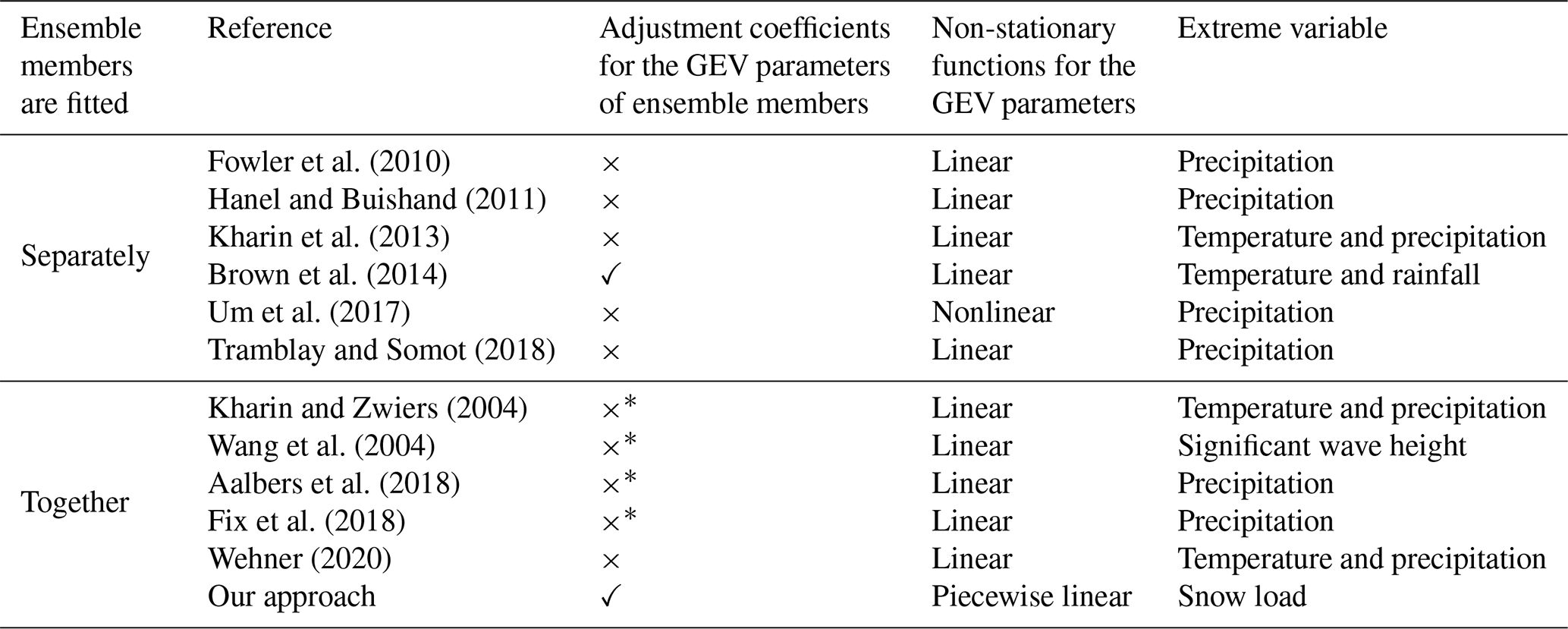
Fowler et al. (2010)Hanel and Buishand (2011)Kharin et al. (2013)Brown et al. (2014)Um et al. (2017)Tramblay and Somot (2018)Kharin and Zwiers (2004)Wang et al. (2004)Aalbers et al. (2018)Fix et al. (2018)Wehner (2020)Table 1Temporal non-stationary GEV-based approaches for GCM ensembles and GCM–RCM ensembles. An asterisk (*) indicates that the ensemble is an initial condition ensemble, i.e., each ensemble member consists of the same GCM–RCM pair with different initializations.
Climate extremes are often assessed within the statistical framework of extreme value theory (EVT) by focusing on either annual maxima or values exceeding a high threshold (Coles, 2001). EVT makes it possible to estimate return levels, i.e., extreme quantiles that occur on average once every T years, where T is the corresponding return period. Return levels play a key role in the design of structures (dams, protections, roofs) to withstand the effects of natural hazards (floods, avalanches, wildfires, snow loads); see, e.g., Rao and Hamed (2000), Eckert et al. (2008), Evin et al. (2018), and Le Roux et al. (2020).
Most approaches using EVT to study climate extremes from multi-model ensembles (MMEs) rely on stationary generalized extreme value (GEV) distributions estimated separately on each climate simulation of the MME, i.e., with each ensemble member (Kharin et al., 2007; Beniston et al., 2007). Specifically, for each ensemble member, annual maxima are assumed stationary for two time periods of 20 or 30 years: one in the historical period representing the late 20th century climate and one in the future period. For instance, Fowler et al. (2007) opted for two 30-year time periods: 1961–1990 and 2071–2100, a 30-year time window corresponding to the usual duration that is used to describe the statistical properties of a climate according to World Meteorological Organization (WMO) standards. Next, stationary 20- or 30-year return levels are estimated for each time period with a GEV distribution. Finally, average changes, i.e., differences in return levels between time periods averaged on all ensemble members, are usually reported (Kharin et al., 2013; O'Gorman, 2014). However, such approaches based on stationary GEV distributions have several drawbacks. First, the assumption of stationarity for 20 or 30 consecutive annual maxima can be debatable, and the possibility of a trend within the 20- or 30-year time periods is often not checked (Kharin and Zwiers, 2004). In addition, the choice to rely only on 20 or 30 maxima implies that the estimated GEV parameters have large uncertainties due to the small number of values used. In this case, large return levels, e.g., the 50-year (or even larger) return periods that are usually considered to design structures (see, e.g., Table 1 of Cabrera et al., 2012), can be highly uncertain.
Temporal non-stationary GEV approaches address these limitations by taking into account all the available annual maxima for each ensemble member, i.e., all the historical and future annual maxima are fitted with a single statistical model (Kharin and Zwiers, 2004). Such approaches combine a stationary random component (a fixed extreme value distribution) with non-stationary deterministic functions that map each temporal covariate (such as the years or the global mean temperatures) to the changing parameters of the distribution. Another advantage of temporal non-stationary approaches is that they allow return levels to be estimated conditionally on each temporal covariate (Kharin et al., 2013).
A majority of temporal non-stationary approaches for MMEs rely on the GEV distributions estimated separately with each climate simulation of the MME (Table 1), with some exceptions (Caires et al., 2006; Kyselý et al., 2010; Roth et al., 2014; Winter et al., 2017), and report return levels (conditionally on a given covariate) averaged on all ensemble members. We believe that such approaches are sub-optimal because they estimate one non-stationary GEV distribution with each climate simulation of the MME, i.e., with fewer than roughly 200 maxima values, which often implies a simple parameterization (linear) for the non-stationary functions (Table 1).
The present study introduces an alternative approach that relies on a temporal non-stationary GEV model fitted to all ensemble members. This approach enables us to quantify uncertainties using standard tools from non-stationary extreme value analysis. Such an approach has mainly been proposed for initial condition ensembles (Table 1), i.e., ensemble members that consist of replicates from the same GCM–RCM pair (or the same GCM for GCM ensembles) simulated with different initial conditions. For initial condition ensembles, this alternative approach estimates a single non-stationary distribution on all ensemble members by assuming that they are independent and identically distributed (iid). However, this alternative approach is inadequate for GCM–RCM ensembles with several GCMs because the iid assumption, i.e., that all GCM–RCM pairs follow the same non-stationary distribution, is unlikely to hold in all the cases. Our study fills this gap with a novel non-stationary extreme value approach inspired by the recent trend of statistical methods that constrain climate projections using past observations (Brunner et al., 2020). We propose to fit a non-stationary GEV distribution to past observations and all GCM–RCM pairs without necessarily assuming that all GCM–RCM pairs follow the same distribution. To this end, we introduce parameters (so-called adjustment coefficients) for the location and scale parameters of the GEV distribution that can account for systematic differences between the different climate trajectories. Different parameterizations of these adjustment coefficients are tested in order to describe the variability between the climate trajectories, the best parameterization being selected using split-sample tests on past observations.
Besides, non-stationary GEV-based approaches for climate projection ensembles usually consider linear functions for the non-stationary functions, with the exception of the study by Um et al. (2017) that applies nonlinear functions (Table 1). In this study, we extend these approaches by considering piecewise linear functions for the non-stationary functions.
We illustrate the proposed methodology with an application to snow load data, which corresponds to the pressure exerted by accumulated snow on the ground (proportional to the snow water equivalent). The probabilistic assessment of ground snow load is of major interest for the structural design of buildings (Croce et al., 2018), for water resource management (Marty et al., 2017), or for the prevention of large-scale environmental or infrastructure damage caused by snow storms (e.g., damage to forests, transportation networks and electricity networks). Since annual means of snow loads are expected to decrease under future climate change, it could be expected that extreme snow load would also decrease. However, in cold regions (high-elevation regions for instance) extreme snowfall is expected to increase with climate change (O'Gorman, 2014), and this increase in extreme snowfall can possibly lead to an increase in extreme snow load. This application verifies whether snow load extremes are expected to decrease in the French Alps, a quantification of these decreases being of prime interest to the study of compound extremes, e.g., extreme snow load combined with extreme wind, or to adapt structures standards, e.g., to decrease the constraints used to design new structures (Le Roux et al., 2020).
Section 2 presents our data, i.e., the 20 GCM–RCM pairs for Representative Concentration Pathway (RCP) 8.5 adjusted from EURO-CORDEX, and the S2M reanalysis set as the reference observational dataset (Vernay et al., 2019, 2022). In Sect. 3, we detail our statistical methodology. Finally, results, discussions and conclusions are introduced in Sects. 4, 5 and 6, respectively.
Our application focuses on snow loads at 1500 m elevation in the 23 massifs of the French Alps, i.e., between Lake Geneva to the north and the Mediterranean Sea to the south (Fig. 1). This region, home to the largest ski resorts in the world, is prone to snow-related hazards, such as avalanches (Favier et al., 2016; Dkengne Sielenou et al., 2021), which are heavily impacted by ongoing warming (Eckert et al., 2013; Castebrunet et al., 2014). This study estimates potential changes in snow load (i.e., the pressure exerted by the snow) hazard for a high-emission scenario (RCP8.5) as a case study, although it could also be applied to other scenarios and variables. Snow load can be defined as the gravitational acceleration (g=9.81 m s−2) times the snow water equivalent (in kg m−2) and is often expressed in units of kN m−2. Snow water equivalent corresponds to the mass of snow per unit surface area, which also corresponds to the observed depth of accumulated snow (in m) multiplied by the snow density (in kg m−3). Following the block maxima approach to estimate the hazard of snow load (Sect. 3.1), we compute annual maxima of daily snow load at 1500 m centered on the winter season, e.g., an annual maximum for the year 1959 is the maximum from 1 August 1958 to 31 July 1959 (Fig. 1).
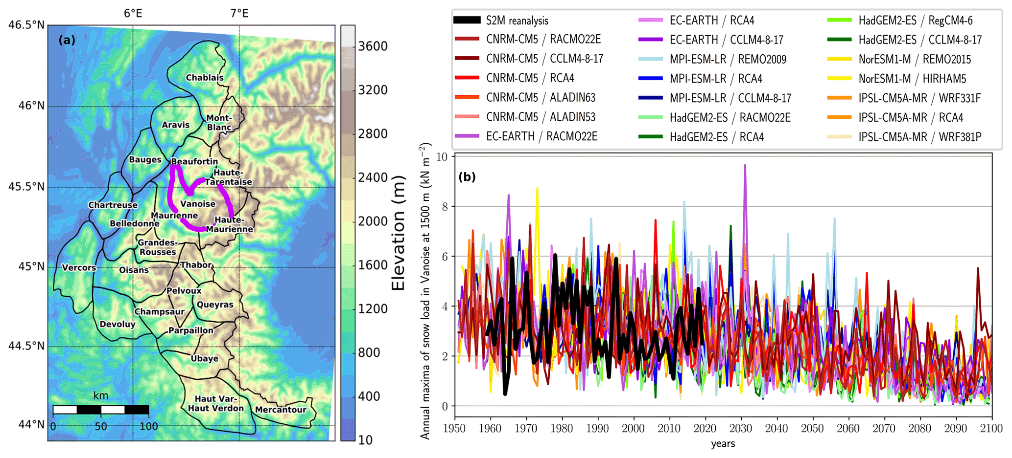
Figure 1(a) Topography and delineation for the 23 massifs of the French Alps, e.g., the Vanoise Massif corresponds to the purple region (Durand et al., 2009). (b) Time series of annual maxima of daily snow load from 1951 to 2100 for the Vanoise Massif at 1500 m elevation. Annual maxima from the S2M reanalysis (1959–2019) are displayed in black, while annual maxima from the 20 adjusted GCM–RCM pairs (1951–2100) under a historical and a high-emission scenario (RCP8.5) are displayed with brighter colors.
The S2M reanalysis (Durand et al., 2009; Vernay et al., 2019, 2022) combines large scale reanalyses and forecasts with in situ meteorological observations to provide daily values of snow load from 1959 to 2019. The S2M reanalysis has been evaluated with both in situ temperature and precipitation observations (Durand et al., 2009) and various snow depth observations (Vionnet et al., 2016; Quéno et al., 2016; Revuelto et al., 2018; Vionnet et al., 2019; Vernay et al., 2022). The S2M reanalysis focuses on the elevation dependency of meteorological conditions. Indeed, this reanalysis is not produced on a regular grid but provides data for each massif every 300 m of elevation between 600 and 3600 m.
ADAMONT (Verfaillie et al., 2017) is a bias-correction and downscaling method that aims to adjust daily climate projections from a regional climate model against a regional reanalysis of hourly meteorological conditions using quantile mapping. This method was used to adjust the EURO-CORDEX dataset (Jacob et al., 2014) against the S2M reanalysis to provide daily values of snow load that spans historical (1951–2005) and future (2006–2100) time periods. Specifically, the EURO-CORDEX dataset consists of RCMs forced over Europe by GCMs from the CMIP5 ensemble (Taylor et al., 2012) for the historical scenario and several representative concentration pathway (RCP) scenarios (Moss et al., 2010). We focus on the RCP8.5 emission scenario and consider a total of 20 GCM–RCM pairs, with 6 GCMs and 11 RCMs total (see Supplement, Table S1). Finally, adjusted EURO-CORDEX meteorological data are used as input to the snow cover model Crocus (Vionnet et al., 2012) every 300 m of elevation for each massif. This provides estimates of the time evolution of the snow cover (Verfaillie et al., 2018), enabling us to compute the maximum annual value of snow load at 1500 m elevation. For simplicity, we often refer to the S2M reanalysis as our observation reference. We note that we discard the two most southern massifs because many projected annual maxima are equal to zero.
The anomaly of global mean surface temperature (GMST) with respect to the pre-industrial period (1850–1900) is chosen as the temporal covariate for our statistical methodology. In practice, we smooth this anomaly with cubic splines to obtain a covariate that does not depend on the internal variability of GMST (Fig. 2). For each GCM–RCM pair we rely on the GMST corresponding GCM as a covariate, while we rely on GMST from HadCRUT5 (Morice et al., 2021) as a covariate for the observations. For simplicity, we refer to +1 ∘C of smoothed anomaly of GMST as +1∘ of global warming.
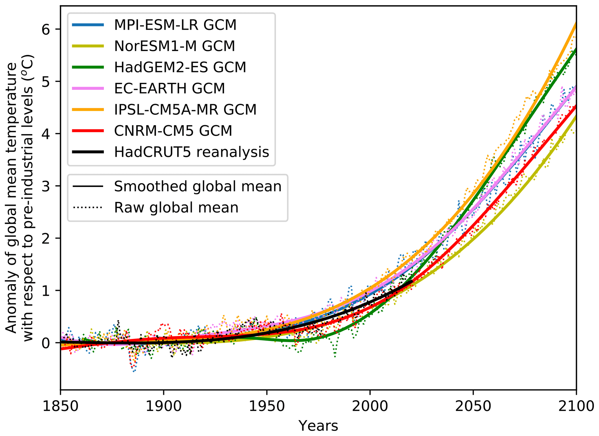
Figure 2Raw output (dotted lines) and smoothed output (plain lines) for the anomaly of global mean annual temperature with respect to industrial levels (1850–1900). For the six GCMs, we show the anomaly of global mean surface temperature using historical emissions until 2005 and projected emissions (RCP8.5). Years correspond to periods centered on each winter (August–July).
3.1 Generalized extreme value distribution
Following the block maxima approach of extreme value theory (Coles, 2001), we model annual maxima with the GEV distribution. Indeed, similarly to the central limit theorem that motivates to model means obtained from different samples using a normal distribution, the Fisher–Tippett–Gnedenko theorem (Fisher and Tippett, 1928; Gnedenko, 1943) encourages to model maxima using the GEV distribution. In practice, if Y represents an annual maximum, a natural choice to model the distribution of Y is , which implies that
where the three parameters are the location μ, the scale σ>0 and the shape ξ. Three subfamilies of distribution (reversed Weibull, Gumbel and Fréchet) can be derived depending on the sign of the shape parameter (ξ<0, ξ=0 and ξ>0), respectively.
In theory, the GEV distribution is adequate when maxima are computed over blocks of infinite size. In practice, the GEV distribution is usually applied to annual maximal values and has been shown to provide reliable estimates of return levels in many hydrometeorological applications (Coles, 2001; Katz et al., 2002; Cooley, 2012; Papalexiou and Koutsoyiannis, 2013). The T-year return level, which is defined as a daily value yp exceeded each year with probability , corresponds to the 1−p quantile of the GEV distribution In this study, we set as it corresponds to the 50-year return period that is widely used for the designed working life of buildings (Cabrera et al., 2012), specifically for the building standards regarding snow load (Croce et al., 2019).
3.2 Non-stationary distribution
Let denote an observed annual maximum for the year t between 1959 and 2019 and represent the smoothed anomaly of global mean surface temperature (GMST) from HadCRUT5 for the same year t (Sect. 2). We rely on a non-stationary distribution where each GEV parameter is a piecewise linear function of T, which is the smoothed anomaly of GMST. A log link function for the scale parameter is introduced to ease the numerical optimization.
where θ is the vector of parameters for the piecewise-linear functions , corresponds to the number of linear pieces, , and Tmin and Tmax are the minimum and maximum smoothed anomaly of GMST for the period 1951–2100 (Fig. 2). In other words, κ2, …, κL are fixed and equally spaced between Tmin and Tmax and correspond to the L−1 anomalies of smoothed GMST where the line breaks, i.e., where the slope of the piecewise linear functions changes.
For a GCM–RCM pair k between 1 and 20, let represent an annual maximum for the year t between 1951 and 2100 and represent the smoothed anomaly of GMST (Sect. 2) for the corresponding GCM.
where Θ denotes the set of parameters θ and of additional parameters and and where ξ(.) is given in Eq. (2). The parameters and correspond to different adjustment coefficients defined in Table 2. For the K=20 GCM–RCM pairs, these adjustment coefficients are considered for the location and scale parameters and aim at adjusting the distribution of GCM–RCM pairs. Following Brown et al. (2014), we assume that these adjustment coefficients are constant, i.e., the same for historical and future climates. We consider five parameterizations: zero adjustment coefficients, one adjustment coefficient for all GCM–RCM pairs, one adjustment coefficient for each GCM, one adjustment coefficient for each RCM and one adjustment coefficient for each GCM–RCM pair. Figure 3 illustrates this concept for a fictive ensemble composed of four different GCM–RCM pairs with two different GCMs and two different RCMs. The right column shows how these adjustment coefficients improve the agreement between the different climate simulations with respect to the observations by removing these first-order discrepancies. Obviously, the parameterization with one additional adjustment coefficient for each GCM–RCM pair leads to a better agreement, but this is at the cost of a much higher number of parameters.

Figure 3Illustration of the evolution of the location parameter μ(T) on the y axis as a function of the global warming T on the x axis for the different options of adjustment coefficients for a fictive ensemble composed of four different GCM–RCM pairs with two different GCMs and two different RCMs. (a) Location parameter μ(T) if the GEV model is fitted individually to each trajectory. (b) Location parameter using adjustment coefficients.
Table 2The five parameterizations of the adjustment coefficients and considered for the location and scale parameters, respectively. When there is only one coefficient for all GCM–RCM pairs k, and for any pair k. When there is one coefficient per GCM (per RCM), and ( and ), where g and r are subscripts referring to the GCM and RCM of the pair k, respectively.
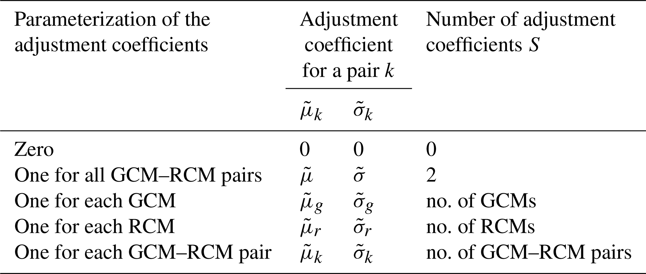
Finally, the size of the entire vector of parameters Θ is , corresponding to three parameters for the intercepts (), 3×L parameters for the piecewise linear functions describing the temporal evolution of the three GEV parameters (see Eq. 2) and S parameters corresponding to the adjustment coefficients (see Table 2).
We did not consider adjustment coefficients on the shape parameter because it sometimes leads to prediction failures. This situation can happen when ξ(T)<0, which means that the predictive distribution has an upper bound, and when some future annual maxima lies above this upper bound.
3.3 Maximum likelihood estimation
For each massif, a temporal non-stationary GEV distribution, parameterized by a vector of coefficients Θ, is estimated using the past observations and all GCM–RCM pairs. Let represent a vector with all annual maxima of a given massif, i.e., annual maxima from the observations and from the K=20 GCM–RCM pairs (Sect. 2). The maximum likelihood method provides the most likely parameters with respect to y. The maximum likelihood estimator is obtained from the past observations and all GCM–RCM pairs by maximizing the following likelihood p(y|Θ):
3.4 Evaluation experiments
Our first evaluation experiment is a model-as-truth experiment, i.e., a perfect model experiment, which evaluates long-term predictive performances using future projections (Abramowitz et al., 2019). The observations from the S2M reanalysis (Sect. 2) are discarded for this experiment. Instead, a simulation from a GCM–RCM pair is chosen as pseudo-observations. The calibration set contains the “historical” data (1959–2019) of the GCM–RCM pair chosen as pseudo-observations and the 19 remaining GCM–RCM pairs (1951–2100). The predictive performance is evaluated on an evaluation set that contains the future data (2020–2100) of the GCM–RCM pair chosen as pseudo-observations. In detail, each GCM–RCM pair is successively regarded as being pseudo-observations. Thus, a model-as-truth experiment can be roughly regarded as a leave-one-out cross-validation with respect to GCM–RCM pairs. We note that for GCM–RCM pairs with the GCM HadGEM2-ES starts in 1982, while the pairs with the RCM RCA4 starts in 1971. Therefore, we successively regard the 12 GCM–RCM pairs (out of 20) that start before 1959 as pseudo-observations, i.e., those that have annual maxima for the period 1959–2019.
Our second evaluation experiment is a split-sample experiment, i.e., a calibration–validation experiment, which enables us to estimate the short-term predictive performance of each parameterization. Specifically, for the calibration of the non-stationary GEV distribution, we rely on the oldest observations from the S2M reanalysis (Sect. 2) and all the GCM–RCM pairs. We validate the predictive performance on the most recent observations. For instance, if we choose to keep 80 % of the observations for the calibration (1959–2007), then the remaining 20 % of the observations are held-out for the evaluation (2008–2019).
In these two evaluation experiments for GCM–RCM ensembles, we calculate the mean logarithmic score () on the evaluation set (the lower the better) to assess the out-of-sample skill of a non-stationary distribution parameterized with the parameter set obtained with the calibration set. The logarithmic score is a proper score that can be used to evaluate the predictive performance of the fitted model (Gneiting et al., 2007). For N out-of-sample observations (or pseudo-observations for the model-as-truth experiment) , we have that where .
3.5 Workflow
First, for a set of past and projected annual maxima, we select one parameterization of the GEV distribution (number of linear pieces, parameterization of the adjustment coefficients) using a two-step selection method: (i) we select the number of linear pieces with a model-as-truth experiment using zero adjustment coefficients for the GEV parameters, and (ii) we then select the parameterization of the adjustment coefficients with three split-sample experiments where the calibration set is composed of 60 %, 70 % and 80 % of the observations, using the number of linear pieces selected in the model-as-truth experiment. Following this, we study trends in the 50-year return level of snow load. For each massif we rely on the parameterization of the GEV distribution selected using the two-step selection method. We report RL50, the 50-year return level that corresponds to Eq. (2), i.e., to the 50-year return level of the observations and their adjusted projections with respect to GCM–RCM pairs. In other words, if the selected parameterization has adjustment coefficients, we do not add these coefficients to compute RL50, since adding these coefficients would provide the 50-year return level of the GCM–RCM pairs. The 90 % confidence interval is computed using a semi-parametric bootstrap resampling method adapted to non-stationary extreme value distributions (Appendix A). For every anomaly of global mean temperature T, we have that the 50-year return level RL50(T) is
4.1 Selection of one parameterization of the GEV distribution for each massif
In Fig. 4a, for each massif we illustrate the selected parameterization of the GEV distribution (number of linear pieces, parameterization of the adjustment coefficients). Among the 23 massifs, Fig. 4b and c highlights the preferred parameterizations after the application of the two-step selection method.
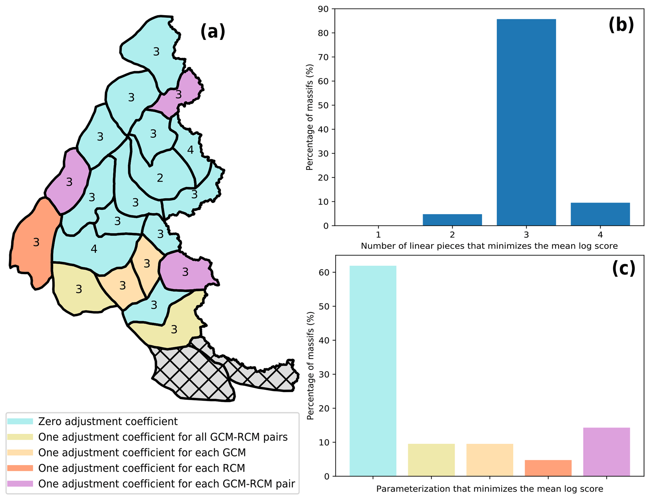
Figure 4(a) Map of the selected parameterization of the GEV distribution at 1500 m. The selected parameterizations of the adjustment coefficients are illustrated with colors, while the selected numbers of linear pieces are written on the map. (b) Distribution of the selected number of linear pieces. (c) Distribution of the selected parameterization of the adjustment coefficients.
In the first step, we select the number of linear pieces that minimizes the mean logarithmic score of a model-as-truth experiment using zero adjustment coefficients for the GEV parameters. The mean logarithmic score is averaged on the hold-out pseudo-observations (2020–2100) for each of the 12 GCM–RCM pairs (which are set as pseudo-observations; see Sect. 4.1). We find that the parameterization with three linear pieces minimizes the mean logarithmic score for 80 % of the massifs, see Fig. 4b. The parameterization with two linear pieces is selected for one massif, and the one with four linear pieces is selected for two massifs. Thus, at least two linear pieces are selected for the piecewise linear functions. In the second step, we select the parameterization of the adjustment coefficients (Table 2) that minimizes the mean logarithmic score for a split-sample experiment using the number of linear pieces selected in the model-as-truth experiment. The mean logarithmic score is averaged on the evaluation observations for three split-sample experiments, where the calibration set corresponds to 60 %, 70 % and 80 % of the observations. Indeed, we observe that the split-sample experiment is quite sensitive to the size of the calibration set. Thus, we choose to average the mean logarithmic score on three split-sample experiments to obtain more robust results. We find that the parameterization with zero adjustment coefficients minimizes the mean logarithmic score for two-thirds of the massifs; see Fig. 4c. Otherwise, the parameterization with one adjustment coefficient for all GCM–RCM pairs is selected for two massifs, the parameterization with one adjustment coefficient for each GCM is selected for two massifs, the parameterization with one adjustment coefficient for each RCM is selected for one massif and the parameterization with one adjustment coefficient for each GCM–RCM pair is selected for three massifs. Thus, for two-thirds of the massifs, adjustment coefficients do not lead to a better predictive performance on the validation periods. This is presumably due to the fact that GCM–RCM pairs have already been statistically adjusted.
A detailed analysis of the mean logarithmic scores of each parameterization for each massif is provided the Supplement.
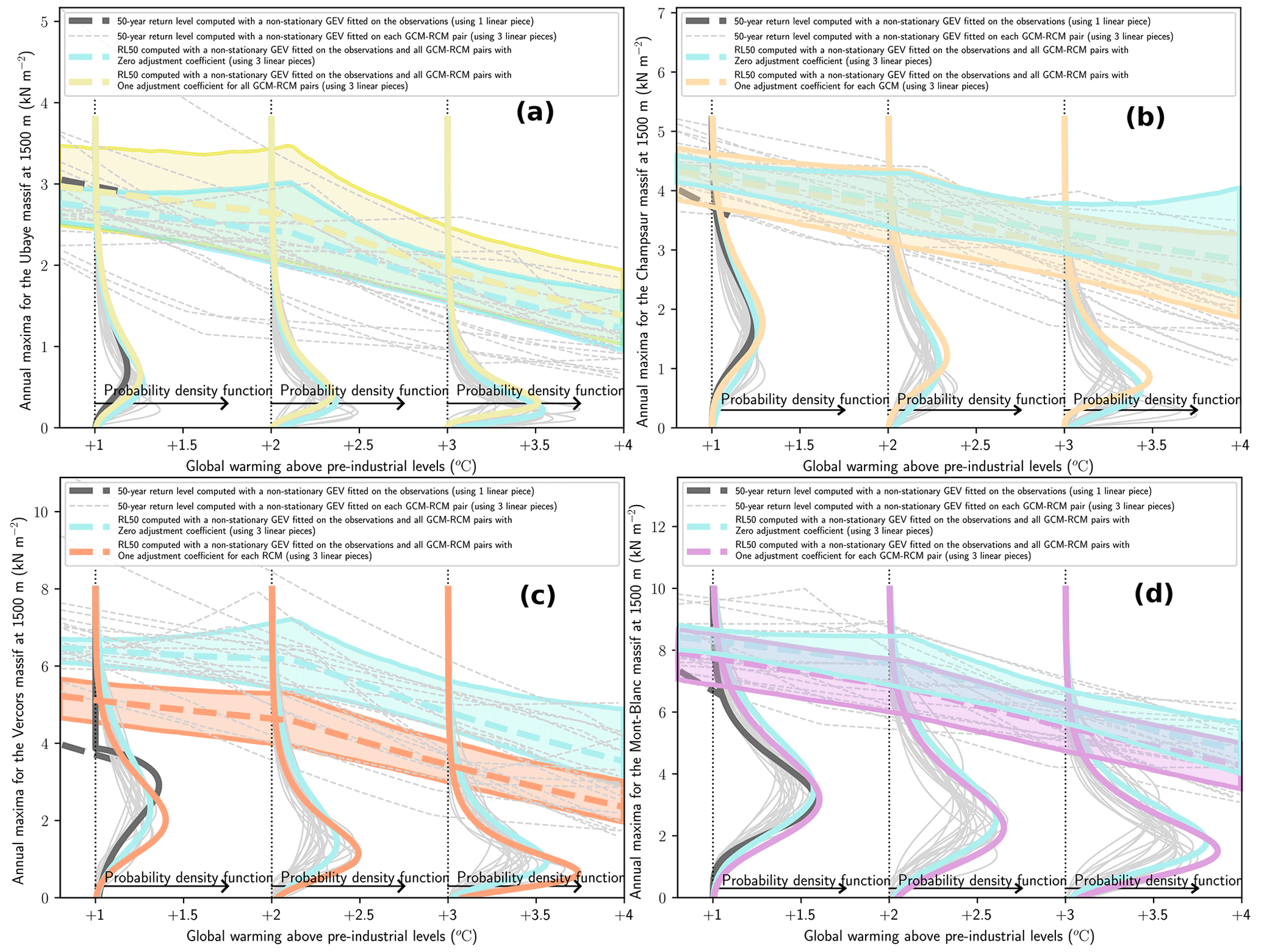
Figure 5Estimated 50-year return levels between +1 and +4 ∘C of global warming at elevation 1500 m under RCP8.5 for four massifs with different preferred parameterizations for the adjustment coefficients: (a) one coefficient for all GCM–RCM pairs, (b) one coefficient for each GCM, (c) one coefficient for each RCM and (d) one coefficient for each GCM–RCM pair. RL50 (Eq. 5) values without adjustment coefficients are shown in cyan, and those with adjustment coefficients are shown in a warm color. The 90 % confidence intervals are shaded. The 50-year return levels computed for each GCM–RCM pair (using a non-stationary GEV distribution with the selected number of linear pieces for each GCM–RCM pair) and for the observation (using a non-stationary GEV distribution with one linear piece and a constant shape parameter) are displayed with thin gray lines and thick dark lines, respectively. The probability density functions at +1, +2 and +3 ∘C exemplify how adjustment coefficients can adjust the distribution.
4.2 Trends in the 50-year return level of snow load
In this section, we rely on the parameterization of the GEV distribution selected in Sect. 4.1 for each massif. In Figure 5, we illustrate changes in the 50-year return level between +1 and +4 ∘C of global warming for four massifs where the selected parameterization is composed of three linear pieces with one adjustment coefficient for all GCM–RCM pairs (Fig. 5a), one coefficient for each GCM (Fig. 5b), one coefficient for each RCM (Fig. 5c) or one coefficient for each GCM–RCM pair (Fig. 5d). In addition, we also perform individual fitting to each GCM–RCM pair, the corresponding return levels being shown with thin gray lines. Note that these estimates are shown for illustrative purposes only, and they do not contribute to the final return level estimates indicated with warm colors.
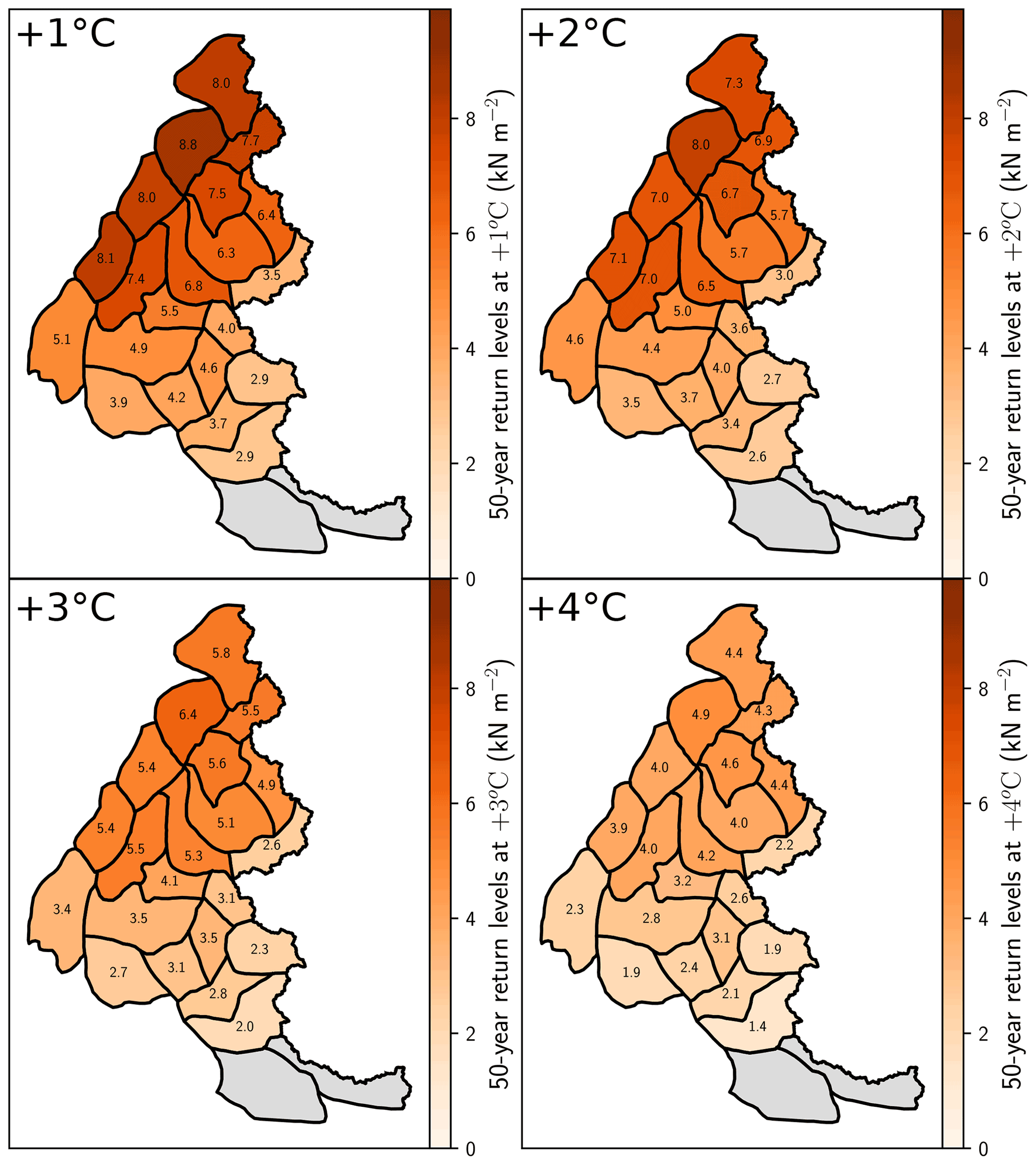
Figure 6The 50-year return levels (RL50) of snow load at 1500 m for +1, +2, +3 and +4 ∘C of global warming under RCP8.5.
All 50-year return levels (for the non-stationary GEV distribution fitted on the observations, on each GCM–RCM pair, and on the observations and all GCM–RCM pairs) are decreasing with the anomaly of global mean temperature. We observe that RL50 with adjustment coefficients (shown in a warm color) is closer to the 50-year return level of the observation (in dark gray) than RL50 without adjustment coefficients (in cyan). This figure also shows how adjustment coefficients adjust the distribution toward the distribution of the observations by illustrating the probability density functions (with and without adjustment) at +1∘ of global warming. Nevertheless, we note that adjusted distributions do not perfectly match the distributions of the observation, which means that the adjusted RL50 does not match the 50-year return levels of the observation. This is probably because we do not consider adjustment coefficients on the shape parameter. For instance, in Fig. 5c, we observe that the shape parameter is negative for the distribution of the observation (because the density has an upper bound), while the shape parameter is positive for the adjusted distribution in orange. We choose to not consider adjustment for the shape parameter because it enables us to constrain predictive distributions on the future period and to avoid prediction failures (Sect. 5.2). Besides, the 90 % confidence interval of RL50 is computed using a semi-parametric bootstrap resampling method adapted to non-stationary extreme distributions (Appendix A). We note that confidence intervals are widening at the nodes of the piecewise linear functions, i.e., at the anomaly of global temperature where the slope of the GEV parameters changes (κi in Eq. 2). This is presumably due to the fact that the variability of the three GEV parameters is more important at the nodes than between them.
Figure 6 illustrates RL50 for the 23 massifs of the French Alps at 1500 m elevation for +1, +2, +3 and +4 ∘C of global warming, i.e., of smoothed anomaly of global mean surface temperature. The return levels are larger in the northwest of the French Alps, and this pattern persists with global warming. Over the whole area of the French Alps, the average RL50 equals 5.7 kN m−2 at +1 ∘C of global warming and 3.3 kN m−2 at +4 ∘C.
Figure 7 details the relative change of RL50 for +2, +3 and +4 ∘C of global warming at 1500 m elevation with respect to +1 ∘C, which corresponds roughly to the current level of global warming above industrial levels (see Fig. 2). Over the French Alps, the average change of RL50 is equal to −0.6 kN m−2 (−10 %), −1.5 kN m−2 (−27 %) and −2.5 kN m−2 (−43 %) for +2, +3 and +4 ∘C of global warming, respectively. These relative changes are different for other elevations, a smaller relative decrease being obtained at 2100 m of elevation and a larger relative decrease at 900 m of elevation (see Supplement B). This result is consistent with the literature (Fig. 2.3 of Hock et al., 2022). At 1500 m, the relative decrease is lower in the central eastern side of the French Alps. For instance, for +4 ∘C of global warming, the relative decrease roughly ranges between −33 % and −38 % in the central eastern side, while it ranges between −40 % and −54 % in the rest of the French Alps.
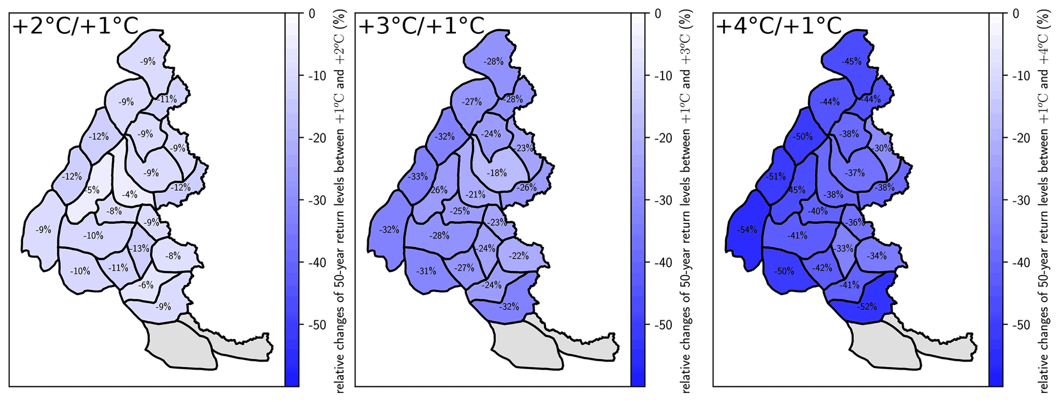
Figure 7Relative changes in 50-year return levels (RL50) of snow load at 1500 m for +2, +3 and +4 ∘C of global warming under the scenario RCP8.5 with respect to +1 ∘C of global warming.
For each massif, it is also possible to compute the average 50-year return level for several time periods: 1986–2005, 2031–2050 and 2080–2099. For instance, for the time period 1986–2005, the average return level equals the average of the return level found for the years 1986, 1987, …, 2005. In order to compute the return level of a given year, e.g., 1986, we rely on the relationship between the anomaly of global mean surface temperature (GMST) and the years (Fig. 2). Specifically, we rely on the anomaly of GMST averaged on the six GCMs to compute this relationship. Following this method, we find that on average the 50-year return level is projected to decrease by −0.8 kN m−2 (−14 %) between 1986–2005 and 2031–2050 and by −2.9 kN m−2 (−50 %) between 1986–2005 and 2080–2099 under the scenario RCP8.5. Note that this method could also provide the rate of change of other RCPs for various lead times using their corresponding global temperature values.
5.1 Comparison of our results with the projected trends at the scale of the European Alps
In Table 3, we compare our results with Fig. 2.31 of Hock et al. (2022) that provides the trends in winter mean snow water equivalent (SWE) at the scale of the European Alps between 1000 and 2000 m under the scenario RCP8.5. As detailed in Sect. 2, the snow load is proportional to the SWE, as it is equal to the SWE times the gravitational acceleration (g=9.81 m s−2).
Hock et al. (2022)Table 3Projected trends in snow water equivalent (SWE) and snow load under the scenario RCP8.5 using the EURO-CORDEX experiment. In the first four rows of the table, we specify that the result is approximated because the trend was read from the Fig. 2.3 of Hock et al. (2022).
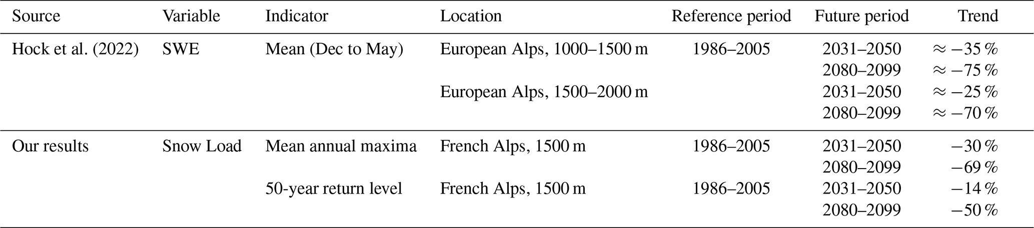
For the 23 massifs, the average return level for several time periods (1986–2005, 2031–2050, 2080–2099) can be obtained as explained in Sect. 4.2. Likewise, the mean annual maxima can be expressed with a similar methodology as the expectation of the non-stationary GEV distribution averaged for each year of the time periods. We find a decrease in mean annual maxima of snow load of −30 % and −69 % for the future periods 2031–2050 and 2080–2099, respectively, compared to the reference period 1986–2005.
Figure 2.3 of Hock et al. (2022) relies on the raw (without adjustment) EURO-CORDEX data. They also find decreasing trends. For instance, between 1500 and 2000 m elevation, the mean winter SWE (proportional to the mean winter snow load) is expected to approximately decrease by −25 % and −70 % for the periods 2031–2050 and 2080–2099, respectively (Table 3). We observe that our mean annual maxima of snow load has a decreasing rate comparable to the decreasing rate of the mean value of snow load. These comparable rates may stem from the fact that (i) both approaches rely (directly or indirectly) on the EURO-CORDEX data or that (ii) the annual maxima of snow load results from an accumulation during the winter (December to May), which implies that we can expect that the mean value will roughly decrease at the same rate as the mean annual maxima.
5.2 Methodological choices, assumptions and limitations
For the non-stationarity of the GEV parameters, we choose piecewise linear functions because they can approximate more complex functions with only a few parameters. This makes our methodology widely applicable. One limitation is that the nodes of the piecewise linear functions are fixed. However, we are confident that these functions are well estimated, owing to the large number of maxima: each of the K=20 GCM–RCM pairs provides more than 100 maxima. Otherwise, we rely on the anomaly of global mean temperature as a covariate (Sect. 2), as do the majority of references cited in Table 1. Indeed, this anomaly is often thought as a good proxy to measure the level of climate change (Fix et al., 2018), which helps strengthen the global response to this threat (Masson-Delmotte et al., 2018). We choose to focus on the scenario RCP8.5 to have the broadest spectrum of potential changes for the 50-year return level of snow load. Also, to obtain Eq. (4) we assume that all annual maxima are conditionally independent given the vector of parameters Θ, which is a classical hypothesis. Following the principle of parsimony, we assume that the adjustment coefficients are constant, i.e., the same for historical and future climates. Besides, as mentioned in Sect. 3.2, we did not consider adjustment coefficients for the shape parameter because it sometimes leads to prediction failure, i.e., the predictive distribution gives a null probability to some future annual maxima. This can happen when ξ(T)<0, which means that the predictive distribution has an upper bound, and when some future annual maxima lies above this upper bound. This illustrates the trade-off between (i) matching the distribution on the past period with respect to the available observations and (ii) having assumptions that help to constrain the predictive distribution on the future period.
For the two-step selection method, we first rely on a model-as-truth experiment to select the number of linear pieces. It assesses the optimal number of linear pieces to predict annual maxima of the pseudo-observations for the evaluation set (2020–2100), i.e., to find a good trade-off between underfitting and overfitting for the calibration set. In this first step, adjustment coefficients are not considered, such that this experiment does not depend on a specific parameterization.
Following this, the best parameterization of the adjustment coefficients is selected with a split-sample experiment. It assesses whether applying adjustment coefficients helps to predict observations of the evaluation set, i.e., whether it is reasonable to assume that the observations do not follow the same distribution as the GCM–RCM pairs. The evaluation score is average for three split-sample experiments where the evaluation set corresponds to the last 40 %, 30 % and 20 % of the observations (Sect. 4.1). Thus, evaluation sets of the three split-sample experiments contain 24, 17 12 annual maxima, respectively, which is a limited amount of information to use for the selection of the best parameterization of the adjustment coefficients. As shown in Fig. 4, it tends to favor the most parsimonious parameterization with no adjustment coefficient. Observed maxima have also a limited effect on the estimated parameters because one observed maxima has the same weight as a maxima from a climate model in the likelihood (Eq. 4). As models are fitted to 61 observed maxima and 20×150 maxima from the different climate models, the selected non-stationary models mostly represent the distribution of the maxima simulated by the climate models. However, it can also be argued that 61 years of past observations has a limited predictive power for long-term horizons where the different trajectories shown by the climate projections can possibly show a great variety of evolution after the observed period. As a comparison, the recent study by Ribes et al. (2021) relies on 170 years of past observations to constrain future climate projections at the global scale. In addition, the proposed methodology has been shown to perform well on temperature projections, but the application to other surface variables (e.g., precipitation, snowfall) needs to be demonstrated.
The 90 % confidence intervals of return levels (Fig. 5) account for both the sampling uncertainty (Appendix A) and the climate model uncertainty (distributions are fitted together from the past observations and all GCM–RCM pairs). In contrast, approaches that estimate return levels separately for each ensemble member usually do not account for the sampling uncertainty, i.e., the sampling uncertainty of return levels estimated on each ensemble, even if this uncertainty can be large because return levels are estimated with only one ensemble member. One limitation of our approach is that, contrary to the climatological expectations, the width of confidence intervals does not increase with global warming (Fig. 5). This is presumably a consequence of assuming constant adjustment coefficients.
The goodness of fit of the selected models has been tested with the application of the Anderson–Darling test (see Appendix A) to each GCM–RCM pair separately and the observations for each massif. The test is rejected for 20% of the 483 cases at a significance level of 5 % (23 massifs × 21 time series). This relatively high number seems to be mainly explained by the small values reached at the end of the century for many GCM–RCM runs. Indeed, the same tests applied at an elevation of 2700 m show a much smaller percentage of rejections (7 %) and larger p values. The inadequacy of the selected GEV models to represent these small values can be related to the high proportion of zero snow load values at the end of the century. In these cases, as annual maxima represent maxima of a limited number of positive values, the asymptotic nature of the extreme value theory might be not respected. One alternative could be to consider larger block sizes (maxima over several years). However, the smaller sample sizes would lead to more uncertain parameter estimates. The application of extreme value models to bounded variables thus remains a substantial challenge, especially in a context of climate change where this issue only affects a small part of the dataset.
5.3 Related works
First, our methodology based on adjustment coefficients can be seen as an extension of Brown et al. (2014), which estimates non-stationary GEV distribution simultaneously with both observations and a single GCM–RCM pair and introduces constant bias terms for each GEV parameter. There are also some links to a debiasing method proposed for annual maxima from GCM–RCM projections (Fontolan et al., 2019). For the location parameter, we consider additive adjustment coefficients that can be seen as bias terms, while the adjustment coefficients of the scale parameter that are multiplicative (due to the log link function) can be viewed as bias-correction factors (Hosseinzadehtalaei et al., 2021). In this paper, we choose the name “adjustment coefficients” because we introduce them to improve the statistical adjustments. Our idea to add adjustment coefficients for each GCM, RCM or GCM–RCM pair into the non-stationary extreme value distributions (Table 2) comes from the ANOVA framework, which can be applied to partition the uncertainty of GCM–RCM projections by identifying the main effects of GCMs and RCMs or GCM–RCM interactions (Hawkins and Sutton, 2009; Evin et al., 2019, 2021).
Thus, our approach based on piecewise linear functions for the non-stationarity of the GEV parameters can be viewed as using linear splines. In the literature, there are many extreme value theory approaches using splines. For instance, linear splines have been applied to model the temporal non-stationarity (Wilcox et al., 2018), while cubic splines are often considered to model spatial extremes (Chavez-Demoulin and Davison, 2005; Gaume et al., 2013).
Following statistical methods that constrain climate projections using past observations (Brunner et al., 2020; Ribes et al., 2021), we propose a novel approach for GCM–RCM ensembles that aims at fitting a single non-stationary generalized extreme value (GEV) distribution to past observations and to the ensemble of GCM–RCM projections. Specifically, we rely on a non-stationary GEV distribution with (i) piecewise linear functions to model the changes in the three GEV parameters and (ii) adjustment coefficients for the location and scale parameters in order to consider the GEV model as adequate for the climate projections and the past observations up to systematic shifts for these two GEV parameters. This wide set of GEV models aims to provide a more flexible framework. In particular, piecewise linear functions can represent many possible future changes of the GEV parameters and include linear trends as special cases.
In order to select the best parameterization of the non-stationary GEV model (number of linear pieces, parameterization of the adjustment coefficients), we design a two-step selection procedure based on two evaluation experiments for GCM–RCM ensembles: a model-as-truth experiment and a split-sample experiment. The model-as-truth experiment is first applied to select the number of nodes that are required to adequately represent the evolution of the GEV parameters. The split-sample experiment evaluates the added value provided by the adjustment coefficients for the different possible parameterizations.
In this article, as a case study the proposed approach is applied to snow load in the French Alps at 1500 m elevation using 20 GCM–RCM pairs that are statistically adjusted from the EURO-CORDEX experiment under the scenario RCP8.5. More generally, the proposed approach could also be applied to other scenarios, climate variables, and climate projection ensembles. In contrast with most applications of non-stationary GEV models in the literature (which consider linear trends), the piecewise linear functions proposed in our approach are well suited to non-monotonic trends.
Many extensions of this work could be considered. First, if adjustment coefficients are not included, our parameterization of the GEV model considers the same non-stationary GEV distribution for the different GCM–RCM pairs. Even in the case where adjustment coefficients are selected, the distributions corresponding to the GCM–RCM pairs are still constrained to have the same changes with global warming because adjustment coefficients are constant. In future work, we could imagine adjustment coefficients that vary with global warming being used to better account for different changes of distributions among the GCM–RCM pairs. A second potential extension of this work could be to improve the parameterization of the GEV distribution by adding weights for each GCM–RCM pair. In our methodology, GCM–RCM pairs are currently considered as equally plausible even though it is known that for each application some of them can have a better agreement with the past observations. Following the intuition of weighting schemes for climate ensemble (Knutti et al., 2017), we could design a parameterization of the GEV distribution that assigns more weight, i.e., more confidence, to climate models that agree more with the observations.
Finally, further work is needed to obtain a better agreement between the non-stationary GEV model representing the ensemble of maxima from climate projections and past observed maxima. Indeed, observed maxima are mainly used to identify and correct strong disagreements between the observed and simulated maxima using adjustment coefficients, and the fitted non-stationary GEV model is not really constrained to represent observed maxima. A Bayesian approach representing the predictive distribution of climate projections conditional on historical observations (Robin and Ribes, 2020; Ribes et al., 2021) could be a possible approach to better constrain a GEV model. However, it requires a long series of past observations to identify the relationships between the forced climate responses to greenhouse gases obtained from the climate models and from the observations.
We estimate the uncertainties resulting from in-sample variability with a semi-parametric bootstrap resampling method adapted to non-stationary extreme distributions (Efron and Tibshirani, 1993; Kharin and Zwiers, 2004). This method relies on a transformation fGEV→standard Gumbel to the standard Gumbel distribution. Indeed, if , then . Let denote a vector of annual maxima, with S the size of the vector. The transformed variates are computed as , using for μ(x), σ(x), ξ(x).
We generate B=1000 bootstrap samples with a four-step procedure. First, we compute the vector . Then, for each bootstrap sample i, from these transformed variates we draw with replacement a sample of size S denoted as , …, . Further, we transform these bootstrapped variates into bootstrapped annual maxima as follows: ∀m, . Finally, we estimate the GEV parameter with the bootstrapped annual maxima . To sum up, this bootstrap procedure provides a set of B GEV parameters that represents the in-sample variability.
In addition to the sampling uncertainty, we also assess the goodness of fit of the fitted GEV models with the Anderson–Darling statistical test (Abidin et al., 2012). If the non-stationary GEV model is adequate, this test assumes that the transformed variates ϵ are drawn from a standard Gumbel distribution. Let Femp and Fgum denote the cumulative distribution functions of the empirical and standard Gumbel distributions, respectively. The Anderson–Darling test is based on the following distance:
where w(x) assigns more weight on the tail of the standard Gumbel distribution (see Abidin et al., 2012, for more details).
The code is publicly available at the following link: https://doi.org/10.5281/zenodo.6769830 (Evin, 2022).
The full S2M reanalysis on which this study is based is freely available from AERIS (Vernay et al., 2019). For each GCM, the global mean surface temperature can be computed from https://climexp.knmi.nl/CMIP5/Tglobal/index.cgi (KNMI, 2022). For the observations, the global mean surface temperature from HadCRUT5 can be downloaded from the following web page: https://www.metoffice.gov.uk/hadobs/hadcrut5/ (last access: 28 June 2022) (Morice et al., 2021).
The supplement related to this article is available online at: https://doi.org/10.5194/esd-13-1059-2022-supplement.
ELR, GE and NE designed the research. ELR performed the analysis and drafted the first version of the manuscript. All authors discussed the results and edited the manuscript.
The contact author has declared that neither they nor their co-authors have any competing interests.
Publisher's note: Copernicus Publications remains neutral with regard to jurisdictional claims in published maps and institutional affiliations.
We are grateful to Ben Youngman for his “evgam” R package. INRAE, CNRM and IGE are members of Labex OSUG. We are indebted to Raphaëlle Samacoïts from Météo France for providing us the latest version of the climate projection data. The authors also thank the editor, Tamas Bodai, Antonio Speranza and an anonymous referee, who provided constructive and useful comments.
This research has been supported by the Institut National de Recherche en Sciences et Technologies pour l'Environnement et l'Agriculture, IRSTEA, which became INRAE in 2020 (PhD grant).
This paper was edited by Valerio Lucarini and reviewed by Tamas Bodai, Antonio Speranza, and one anonymous referee.
Aalbers, E. E., Lenderink, G., van Meijgaard, E., and van den Hurk, B. J.: Local-scale changes in mean and heavy precipitation in Western Europe, climate change or internal variability?, Clim. Dynam., 50, 4745–4766, https://doi.org/10.1007/s00382-017-3901-9, 2018. a
Abidin, N. Z., Adam, M. B., and Midi, H.: The Goodness-of-fit Test for Gumbel Distribution: A Comparative Study, Matematika, 28, 35–48, https://doi.org/10.11113/matematika.v28.n.313, 2012. a, b
Abramowitz, G., Herger, N., Gutmann, E., Hammerling, D., Knutti, R., Leduc, M., Lorenz, R., Pincus, R., and Schmidt, G. A.: ESD Reviews: Model dependence in multi-model climate ensembles: weighting, sub-selection and out-of-sample testing, Earth Syst. Dynam., 10, 91–105, https://doi.org/10.5194/esd-10-91-2019, 2019. a
Beniston, M., Stephenson, D. B., Christensen, O. B., Ferro, C. A., Frei, C., Goyette, S., Halsnaes, K., Holt, T., Jylhä, K., Koffi, B., Palutikof, J., Schöll, R., Semmler, T., and Woth, K.: Future extreme events in European climate: An exploration of regional climate model projections, Climatic Change, 81, 71–95, https://doi.org/10.1007/s10584-006-9226-z, 2007. a
Brown, S. J., Murphy, J. M., Sexton, D. M., and Harris, G. R.: Climate projections of future extreme events accounting for modelling uncertainties and historical simulation biases, Clim. Dynam., 43, 2681–2705, https://doi.org/10.1007/s00382-014-2080-1, 2014. a, b, c
Brunner, L., McSweeney, C., Ballinger, A. P., Befort, D. J., Benassi, M., Booth, B., Coppola, E., de Vries, H., Harris, G., Hegerl, G. C., Knutti, R., Lenderink, G., Lowe, J., Nogherotto, R., O’Reilly, C., Qasmi, S., Ribes, A., Stocchi, P., and Undorf, S.: Comparing Methods to Constrain Future European Climate Projections Using a Consistent Framework, J. Climate, 33, 8671–8692, https://doi.org/10.1175/jcli-d-19-0953.1, 2020. a, b
Cabrera, A. T., Heras, M. D., Cabrera, C., and Heras, A. M. D.: The Time Variable in the Calculation of Building Structures. How to extend the working life until the 100 years?, in: 2nd International Conference on Construction and Building Research, 1–6, http://oa.upm.es/22914/1/INVE_MEM_2012_152534.pdf (last access: 26 June 2022), 2012. a, b
Caires, S., Swail, V. R., and Wang, X. L.: Projection and analysis of extreme wave climate, J. Climate, 19, 5581–5605, https://doi.org/10.1175/JCLI3918.1, 2006. a
Castebrunet, H., Eckert, N., Giraud, G., Durand, Y., and Morin, S.: Projected changes of snow conditions and avalanche activity in a warming climate: The French Alps over the 2020–2050 and 2070–2100 periods, The Cryosphere, 8, 1673–1697, https://doi.org/10.5194/tc-8-1673-2014, 2014. a
Chavez-Demoulin, V. and Davison, A. C.: Generalized additive modelling of sample extremes, J. Roy. Stat. Soc. Ser. C, 54, 207–222, https://doi.org/10.1111/j.1467-9876.2005.00479.x, 2005. a
Coles, S. G.: An introduction to Statistical Modeling of Extreme Values, in: vol. 208, Springer, London, https://doi.org/10.1007/978-1-4471-3675-0, 2001. a, b, c
Cooley, D.: Return Periods and Return Levels Under Climate Change, in: Extremes in a Changing Climate – Detection, Analysis & Uncertainty, Springer Science & Business Media, 97–114, https://doi.org/10.1007/978-94-007-4479-0, 2012. a
Croce, P., Formichi, P., Landi, F., and Marsili, F.: Climate change: Impact on snow loads on structures, Cold Reg. Sci. Technol., 150, 35–50, https://doi.org/10.1016/J.COLDREGIONS.2017.10.009, 2018. a
Croce, P., Formichi, P., Landi, F., and Marsili, F.: Harmonized European ground snow load map: Analysis and comparison of national provisions, Cold Reg. Sci. Technol., 168, 102875, https://doi.org/10.1016/j.coldregions.2019.102875, 2019. a
Dkengne Sielenou, P., Viallon-Galinier, L., Hagenmuller, P., Naveau, P., Morin, S., Dumont, M., Verfaillie, D., and Eckert, N.: Combining random forests and class-balancing to discriminate between three classes of avalanche activity in the French Alps, Cold Reg. Sci. Technol., 187, 103276, https://doi.org/10.1016/j.coldregions.2021.103276, 2021. a
Durand, Y., Laternser, M., Giraud, G., Etchevers, P., Lesaffre, B., and Mérindol, L.: Reanalysis of 44 yr of climate in the French Alps (1958–2002): Methodology, model validation, climatology, and trends for air temperature and precipitation, J. Appl. Meteorol. Clim., 48, 429–449, https://doi.org/10.1175/2008JAMC1808.1, 2009. a, b, c
Eckert, N., Parent, E., Naaim, M., and Richard, D.: Bayesian stochastic modelling for avalanche predetermination: From a general system framework to return period computations, Stoch. Environ. Res. Risk Assess., 22, 185–206, https://doi.org/10.1007/s00477-007-0107-4, 2008. a
Eckert, N., Keylock, C. J., Castebrunet, H., Lavigne, A., and Naaim, M.: Temporal trends in avalanche activity in the French Alps and subregions: From occurrences and runout altitudes to unsteady return periods, J. Glaciol., 59, 93–114, https://doi.org/10.3189/2013JoG12J091, 2013. a
Efron, B. and Tibshirani, R. J.: An introduction to the bootstrap, Chapman and Hall, https://doi.org/10.1201/9780203217252.ch1, 1993. a
Evin, G.: guillaumeevin/pynonstationarygev: pynonstationarygev (v1.0.0), Zenodo [code], https://doi.org/10.5281/zenodo.6769830, 2022. a
Evin, G., Curt, T., and Eckert, N.: Has fire policy decreased the return period of the largest wildfire events in France? A Bayesian assessment based on extreme value theory, Nat. Hazards Earth Syst. Sci., 18, 2641–2651, https://doi.org/10.5194/nhess-18-2641-2018, 2018. a
Evin, G., Hingray, B., Blanchet, J., Eckert, N., Morin, S., and Verfaillie, D.: Partitioning Uncertainty Components of an Incomplete Ensemble of Climate Projections Using Data Augmentation, J. Climate, 32, 2423–2440, https://doi.org/10.1175/JCLI-D-18-0606.1, 2019. a
Evin, G., Somot, S., and Hingray, B.: Balanced estimate and uncertainty assessment of European climate change using the large EURO-CORDEX regional climate model ensemble, Earth Syst. Dynam., 12, 1543–1569, https://doi.org/10.5194/esd-12-1543-2021, 2021. a
Favier, P., Eckert, N., Faug, T., Bertrand, D., and Naaim, M.: Avalanche risk evaluation and protective dam optimal design using extreme value statistics, J. Glaciol., 62, 725–749, https://doi.org/10.1017/jog.2016.64, 2016. a
Fisher, R. A. and Tippett, L. H. C.: Limiting forms of the frequency distribution of the largest or smallest member of a sample, Math. Proc. Cambridge Philos. Soc., 24, 180–190, https://doi.org/10.1017/S0305004100015681, 1928. a
Fix, M. J., Cooley, D., Sain, S. R., and Tebaldi, C.: A comparison of U.S. precipitation extremes under RCP8.5 and RCP4.5 with an application of pattern scaling, Climatic Change, 146, 335–347, https://doi.org/10.1007/s10584-016-1656-7, 2018. a, b
Fontolan, M., Xavier, A. C. F., Pereira, H. R., and Blain, G. C.: Using climate change models to assess the probability of weather extremes events: A local scale study based on the generalized extreme value distribution, Bragantia, 78, 146–157, https://doi.org/10.1590/1678-4499.2018144, 2019. a
Fowler, H. J., Ekström, M., Blenkinsop, S., and Smith, A. P.: Estimating change in extreme European precipitation using a multimodel ensemble, J. Geophys. Res.-Atmos., 112, D18104, https://doi.org/10.1029/2007JD008619, 2007. a
Fowler, H. J., Cooley, D., Sain, S. R., and Thurston, M.: Detecting change in UK extreme precipitation using results from the climateprediction.net BBC climate change experiment, Extremes, 13, 241–267, https://doi.org/10.1007/s10687-010-0101-y, 2010. a
Gaume, J., Eckert, N., Chambon, G., Naaim, M., and Bel, L.: Mapping extreme snowfalls in the French Alps using max-stable processes, Water Resour. Res., 49, 1079–1098, https://doi.org/10.1002/wrcr.20083, 2013. a
Gnedenko, B.: Sur la distribution limite du terme maximum d'une série aléatoire, Ann. Math., 44, 423–453, https://doi.org/10.2307/1968974, 1943. a
Gneiting, T., Balabdaoui, F., and Raftery, A. E.: Probabilistic forecasts, calibration and sharpness, J. Roy. Stat. Soc. Ser. B, 69, 243–268, 2007. a
Hanel, M. and Buishand, T. A.: Analysis of precipitation extremes in an ensemble of transient regional climate model simulations for the Rhine basin, Clim. Dynam., 36, 1135–1153, https://doi.org/10.1007/s00382-010-0822-2, 2011. a
Hawkins, E. and Sutton, R.: The potential to narrow uncertainty in regional climate predictions, B. Am. Meteorol. Soc., 90, 1095–1107, https://doi.org/10.1175/2009BAMS2607.1, 2009. a
Hock, R., Rasul, G., Adler, C., Cáceres, B., Gruber, S., Hirabayashi, Y., Jackson, M., Kääb, A., Kang, S., Kutuzov, S., Milner, A., Molau, U., Morin, S., Orlove, B., and Steltzer, H.: High Mountain Areas, in: IPCC Special Report on the Ocean and Cryosphere in a Changing Climate, edited by: Pörtner, H.-O., Roberts, D. C., Masson-Delmotte, V., Zhai, P., Tignor, M., Poloczanska, E., Mintenbeck, K., Alegría, A., Nicolai, M., Okem, A., Petzold, J., Rama, B., and Weyer, N. M., Cambridge University Press, Cambridge, UK and New York, NY, USA, 131–202, https://doi.org/10.1017/9781009157964.004, 2022. a, b, c, d, e
Hosseinzadehtalaei, P., Ishadi, N. K., Tabari, H., and Willems, P.: Climate change impact assessment on pluvial flooding using a distribution-based bias correction of regional climate model simulations, J. Hydrol., 598, 126239, https://doi.org/10.1016/j.jhydrol.2021.126239, 2021. a
IPCC: Climate Change 2021: The Physical Science Basis, in: Contribution of Working Group I to the Sixth Assessment Report of the Intergovernmental Panel on Climate Change, edited by: Masson-Delmotte, V., Zhai, P., Pirani, A., Connors, S. L., Péan, C., Berger, S., Caud, N., Chen, Y., Goldfarb, L., Gomis, M. I., Huang, M., Leitzell, K., Lonnoy, E., Matthews, J. B. R., Maycock, T. K., Waterfield, T., Yelekçi, O., Yu, R., and Zhou, B., Cambridge University Press, https://www.ipcc.ch/report/sixth-assessment-report-working-group-i/ (last access: 24 June 2022), 2021. a
Jacob, D., Petersen, J., Eggert, B., Alias, A., Christensen, O. B., Bouwer, L. M., Braun, A., Colette, A., Déqué, M., Georgievski, G., Georgopoulou, E., Gobiet, A., Menut, L., Nikulin, G., Haensler, A., Hempelmann, N., Jones, C., Keuler, K., Kovats, S., Kröner, N., Kotlarski, S., Kriegsmann, A., Martin, E., van Meijgaard, E., Moseley, C., Pfeifer, S., Preuschmann, S., Radermacher, C., Radtke, K., Rechid, D., Rounsevell, M., Samuelsson, P., Somot, S., Soussana, J. F., Teichmann, C., Valentini, R., Vautard, R., Weber, B., and Yiou, P.: EURO-CORDEX: New high-resolution climate change projections for European impact research, Reg. Environ. Change, 14, 563–578, https://doi.org/10.1007/s10113-013-0499-2, 2014. a
Katz, R. W., Parlange, M. B., and Naveau, P.: Statistics of extremes in hydrology, Adv. Water Resour., 25, 1287–1304, https://doi.org/10.1016/S0309-1708(02)00056-8, 2002. a
Kharin, V. V. and Zwiers, F. W.: Estimating extremes in transient climate change simulations, J. Climate, 18, 1156–1173, https://doi.org/10.1175/JCLI3320.1, 2004. a, b, c, d
Kharin, V. V., Zwiers, F. W., Zhang, X., and Hegerl, G. C.: Changes in temperature and precipitation extremes in the IPCC ensemble of global coupled model simulations, J. Climate, 20, 1419–1444, https://doi.org/10.1175/JCLI4066.1, 2007. a
Kharin, V. V., Zwiers, F. W., Zhang, X., and Wehner, M.: Changes in temperature and precipitation extremes in the CMIP5 ensemble, Climatic Change, 119, 345–357, https://doi.org/10.1007/s10584-013-0705-8, 2013. a, b, c
KNMI: 2013 Global mean temperature of CMIP5 monthly historical and RCP experiments, KNMI [data set], https://climexp.knmi.nl/CMIP5/Tglobal/index.cgi, last access: 24 June 2022. a
Knutti, R., Sedláček, J., Sanderson, B. M., Lorenz, R., Fischer, E. M., and Eyring, V.: A climate model projection weighting scheme accounting for performance and interdependence, Geophys. Res. Lett., 44, 1909–1918, https://doi.org/10.1002/2016GL072012, 2017. a
Kyselý, J., Picek, J., and Beranová, R.: Estimating extremes in climate change simulations using the peaks-over-threshold method with a non-stationary threshold, Global Planet. Change, 72, 55–68, https://doi.org/10.1016/j.gloplacha.2010.03.006, 2010. a
Le Roux, E., Evin, G., Eckert, N., Blanchet, J., and Morin, S.: Non-stationary extreme value analysis of ground snow loads in the French Alps: a comparison with building standards, Nat. Hazards Earth Syst. Sci., 20, 2961–2977, https://doi.org/10.5194/nhess-20-2961-2020, 2020. a, b
Marty, C., Tilg, A.-M., Jonas, T., Marty, C., Tilg, A.-M., and Jonas, T.: Recent Evidence of Large-Scale Receding Snow Water Equivalents in the European Alps, J. Hydrometeorol., 18, 1021–1031, https://doi.org/10.1175/JHM-D-16-0188.1, 2017. a
Masson-Delmotte, V., Zhai, P., Pörtner, H.-O., Roberts, D., Skea, J., Shukla, P. R., Pirani, A., Moufouma-Okia, W., Péan, C., Pidcock, R., Connors, S., Matthews, J. B. R., Chen, Y., Zhou, X., Gomis, M. I., Lonnoy, E., Maycock, T., Tignor, M., and Waterfield, T.: An IPCC Special Report on the impacts of global warming of 1.5, Cambridge University Press, https://doi.org/10.1017/CBO9781107415324, 2018. a
Morice, C. P., Kennedy, J. J., Rayner, N. A., Winn, J. P., Hogan, E., Killick, R. E., Dunn, R. J., Osborn, T. J., Jones, P. D., and Simpson, I. R.: An Updated Assessment of Near-Surface Temperature Change From 1850: The HadCRUT5 Data Set, J. Geophys. Res.-Atmos., 126, e2019JD032361, https://doi.org/10.1029/2019JD032361, 2021. a, b
Moss, R. H., Edmonds, J. A., Hibbard, K. A., Manning, M. R., Rose, S. K., Van Vuuren, D. P., Carter, T. R., Emori, S., Kainuma, M., Kram, T., Meehl, G. A., Mitchell, J. F., Nakicenovic, N., Riahi, K., Smith, S. J., Stouffer, R. J., Thomson, A. M., Weyant, J. P., and Wilbanks, T. J.: The next generation of scenarios for climate change research and assessment, Nature, 463, 747–756, https://doi.org/10.1038/nature08823, 2010. a
O'Gorman, P. A.: Contrasting responses of mean and extreme snowfall to climate change, Nature, 512, 416–418, https://doi.org/10.1038/nature13625, 2014. a, b
Papalexiou, S. M. and Koutsoyiannis, D.: Battle of extreme value distributions: A global survey on extreme daily rainfall, Water Resour. Res., 49, 187–201, https://doi.org/10.1029/2012WR012557, 2013. a
Quéno, L., Vionnet, V., Dombrowski-Etchevers, I., Lafaysse, M., Dumont, M., and Karbou, F.: Snowpack modelling in the Pyrenees driven by kilometric-resolution meteorological forecasts, The Cryosphere, 10, 1571–1589, https://doi.org/10.5194/tc-10-1571-2016, 2016. a
Rao, A. R. and Hamed, K. H.: Flood Frequency Analysis, CRC Press, https://doi.org/10.1201/9780429128813, 2000. a
Revuelto, J., Lecourt, G., Lafaysse, M., Zin, I., Charrois, L., Vionnet, V., Dumont, M., Rabatel, A., Six, D., Condom, T., Morin, S., Viani, A., and Sirguey, P.: Multi-criteria evaluation of snowpack simulations in complex alpine terrain using satellite and in situ observations, Remote Sens., 10, 1–32, https://doi.org/10.3390/rs10081171, 2018. a
Ribes, A., Qasmi, S., and Gillett, N. P.: Making climate projections conditional on historical observations, Sci. Adv. 7, 1–10, https://doi.org/10.1126/sciadv.abc0671, 2021. a, b, c
Robin, Y. and Ribes, A.: Nonstationary extreme value analysis for event attribution combining climate models and observations, Adv. Stat. Climatol. Meteorol. Oceanogr., 6, 205–221, https://doi.org/10.5194/ascmo-6-205-2020, 2020. a
Roth, M., Buishand, T. A., Jongbloed, G., Klein Tank, A. M., and van Zanten, J. H.: Projections of precipitation extremes based on a regional, non-stationary peaks-over-threshold approach: A case study for the Netherlands and north-western Germany, Weather Clim. Extrem., 4, 1–10, https://doi.org/10.1016/j.wace.2014.01.001, 2014. a
Taylor, K. E., Stouffer, R. J., and Meehl, G. A.: An overview of CMIP5 and the experiment design, B. Am. Meteorol. Soc., 93, 485–498, https://doi.org/10.1175/BAMS-D-11-00094.1, 2012. a
Tramblay, Y. and Somot, S.: Future evolution of extreme precipitation in the Mediterranean, Climatic Change, 151, 289–302, https://doi.org/10.1007/s10584-018-2300-5, 2018. a
Um, M. J., Kim, Y., Markus, M., and Wuebbles, D. J.: Modeling nonstationary extreme value distributions with nonlinear functions: An application using multiple precipitation projections for U.S. cities, J. Hydrol., 552, 396–406, https://doi.org/10.1016/j.jhydrol.2017.07.007, 2017. a, b
Verfaillie, D., Déqué, M., Morin, S., and Lafaysse, M.: The method ADAMONT v1.0 for statistical adjustment of climate projections applicable to energy balance land surface models, Geosci. Model Dev., 10, 4257–4283, https://doi.org/10.5194/gmd-10-4257-2017, 2017. a
Verfaillie, D., Lafaysse, M., Déqué, M., Eckert, N., Lejeune, Y., and Morin, S.: Multi-component ensembles of future meteorological and natural snow conditions for 1500 m altitude in the Chartreuse mountain range, Northern French Alps, The Cryosphere, 12, 1249–1271, https://doi.org/10.5194/tc-12-1249-2018, 2018. a
Vernay, M., Lafaysse, M., Hagenmuller, P., Nheili, R., Verfaillie, D., and Morin, S.: The S2M meteorological and snow cover reanalysis in the French mountainous areas (1958–present), AERIS [data set], https://doi.org/10.25326/37, 2019. a, b, c
Vernay, M., Lafaysse, M., Monteiro, D., Hagenmuller, P., Nheili, R., Samacoïts, R., Verfaillie, D., and Morin, S.: The S2M meteorological and snow cover reanalysis over the French mountainous areas: description and evaluation (1958–2021), Earth Syst. Sci. Data, 14, 1707–1733, https://doi.org/10.5194/essd-14-1707-2022, 2022. a, b, c
Vionnet, V., Brun, E., Morin, S., Boone, A., Faroux, S., Le Moigne, P., Martin, E., and Willemet, J.-M.: The detailed snowpack scheme Crocus and its implementation in SURFEX v7.2, Geosci. Model Dev., 5, 773–791, https://doi.org/10.5194/gmd-5-773-2012, 2012. a
Vionnet, V., Dombrowski-Etchevers, I., Lafaysse, M., Quéno, L., Seity, Y., and Bazile, E.: Numerical weather forecasts at kilometer scale in the French Alps: Evaluation and application for snowpack modeling, J. Hydrometeorol., 17, 2591–2614, https://doi.org/10.1175/JHM-D-15-0241.1, 2016. a
Vionnet, V., Six, D., Auger, L., Dumont, M., Lafaysse, M., Quéno, L., Réveillet, M., Dombrowski-Etchevers, I., Thibert, E., and Vincent, C.: Sub-kilometer Precipitation Datasets for Snowpack and Glacier Modeling in Alpine Terrain, Front. Earth Sci., 7, 1–21, https://doi.org/10.3389/feart.2019.00182, 2019. a
Wang, X. L., Zwiers, F. W., and Swail, V. R.: North Atlantic ocean wave climate change scenarios for the twenty-first century, J. Climate, 17, 2368–2383, https://doi.org/10.1175/1520-0442(2004)017<2368:NAOWCC>2.0.CO;2, 2004. a
Wehner, M. F.: Characterization of long period return values of extreme daily temperature and precipitation in the CMIP6 models: Part 2, projections of future change, Weather Clim. Extrem., 30, 100284, https://doi.org/10.1016/j.wace.2020.100284, 2020. a
Wilcox, C., Vischel, T., Panthou, G., Bodian, A., Blanchet, J., Descroix, L., Quantin, G., Cassé, C., Tanimoun, B., and Kone, S.: Trends in hydrological extremes in the Senegal and Niger Rivers, J. Hydrol., 566, 531–545, https://doi.org/10.1016/J.JHYDROL.2018.07.063, 2018. a
Winter, H.nC., Brown, S. J., and Tawn, J. A.: Characterising the changing behaviour of heatwaves with climate change, Dynam. Stat. Clima. Syst., 1, dzw006, https://doi.org/10.1093/climsys/dzw006, 2017. a
https://www.ipcc.ch/srocc/chapter/chapter-2/2-1introduction/ipcc-srocc-ch_2_3/ (last access: 23 June 2022).
- Abstract
- Introduction
- Data
- Statistical methodology
- Results
- Discussion
- Conclusions and outlook
- Appendix A: Uncertainty assessment and goodness-of-fit test
- Code availability
- Data availability
- Author contributions
- Competing interests
- Disclaimer
- Acknowledgements
- Financial support
- Review statement
- References
- Supplement