the Creative Commons Attribution 4.0 License.
the Creative Commons Attribution 4.0 License.
 | 16 Sep 2021
Coupled regional Earth system modeling in the Baltic Sea region
Matthias Gröger
Christian Dieterich
Jari Haapala
Ha Thi Minh Ho-Hagemann
Stefan Hagemann
Jaromir Jakacki
Wilhelm May
H. E. Markus Meier
Paul A. Miller
Anna Rutgersson
Lichuan Wu
Nonlinear responses to externally forced climate change are known to dampen or amplify the local climate impact due to complex cross-compartmental feedback loops in the Earth system. These feedbacks are less well represented in the traditional stand-alone atmosphere and ocean models on which many of today's regional climate assessments rely (e.g., EURO-CORDEX, NOSCCA and BACC II). This has promoted the development of regional climate models for the Baltic Sea region by coupling different compartments of the Earth system into more comprehensive models. Coupled models more realistically represent feedback loops than the information imposed on the region by prescribed boundary conditions and, thus, permit more degrees of freedom. In the past, several coupled model systems have been developed for Europe and the Baltic Sea region. This article reviews recent progress on model systems that allow two-way communication between atmosphere and ocean models; models for the land surface, including the terrestrial biosphere; and wave models at the air–sea interface and hydrology models for water cycle closure. However, several processes that have mostly been realized by one-way coupling to date, such as marine biogeochemistry, nutrient cycling and atmospheric chemistry (e.g., aerosols), are not considered here.
In contrast to uncoupled stand-alone models, coupled Earth system models can modify mean near-surface air temperatures locally by up to several degrees compared with their stand-alone atmospheric counterparts using prescribed surface boundary conditions. The representation of small-scale oceanic processes, such as vertical mixing and sea-ice dynamics, appears essential to accurately resolve the air–sea heat exchange over the Baltic Sea, and these parameters can only be provided by online coupled high-resolution ocean models. In addition, the coupling of wave models at the ocean–atmosphere interface allows for a more explicit formulation of small-scale to microphysical processes with local feedbacks to water temperature and large-scale processes such as oceanic upwelling. Over land, important climate feedbacks arise from dynamical terrestrial vegetation changes as well as the implementation of land-use scenarios and afforestation/deforestation that further alter surface albedo, roughness length and evapotranspiration. Furthermore, a good representation of surface temperatures and roughness length over open sea and land areas is critical for the representation of climatic extremes such as heavy precipitation, storms, or tropical nights (defined as nights where the daily minimum temperature does not fall below 20 ∘C), and these parameters appear to be sensitive to coupling.
For the present-day climate, many coupled atmosphere–ocean and atmosphere–land surface models have demonstrated the added value of single climate variables, in particular when low-quality boundary data were used in the respective stand-alone model. This makes coupled models a prospective tool for downscaling climate change scenarios from global climate models because these models often have large biases on the regional scale. However, the coupling of hydrology models to close the water cycle remains problematic, as the accuracy of precipitation provided by atmosphere models is, in most cases, insufficient to realistically simulate the runoff to the Baltic Sea without bias adjustments.
Many regional stand-alone ocean and atmosphere models are tuned to suitably represent present-day climatologies rather than to accurately simulate climate change. Therefore, more research is required into how the regional climate sensitivity (e.g., the models' response to a given change in global mean temperature) is affected by coupling and how the spread is altered in multi-model and multi-scenario ensembles of coupled models compared with uncoupled ones.
- Article
(2890 KB) - Full-text XML
- BibTeX
- EndNote


During the preparation of this paper, shortly before acceptance, Christian Dieterich passed away (1964–2021). This sad event marked the end of the life of a distinguished oceanographer and climate scientist who made important contributions to the climate modeling of the Baltic Sea, North Sea and North Atlantic regions.
Climatic and environmental changes on regional scales are traditionally investigated using stand-alone models that resolve processes specific to only one single environmental compartment (e.g., the terrestrial and marine biospheres, the hydrosphere, the atmosphere, the ocean and the cryosphere). Many projections that served as a basis for the recent climate change assessments for the North Sea (NOSCCA; May et al., 2016; Schrum et al., 2016) and Baltic Sea (Bøssing-Christensen et al., 2015, 2021) or the EURO-CORDEX region (Jacob et al., 2014) fall into the category of stand-alone ocean models or stand-alone atmosphere models, whereas fewer assessments have been based on coupled systems (Meier et al., 2015, 2021). However, as environmental compartments interact with each other via mass, momentum and energy exchange, the interfaces and boundary layers between the compartments are of great importance.
The use of Earth system models (ESMs) that interactively couple atmospheric, marine and terrestrial energy, water and biogeochemical dynamics is becoming increasingly common practice in global climate assessments (e.g., IPCC 2013) and international coordinated protocols for climate simulations (e.g., the emission-driven CMIP6-C4MIP; Eyring et al., 2016; Jones et al., 2016). Their employment in regional climate change and impact studies (e.g., Döscher and Meier, 2004; Somot et al., 2008; Wramneby et al., 2010; Meier et al., 2011; Cabos et al., 2020; Sein et al., 2020, Zhang et al., 2018; Soto-Navarro et al., 2020; Dieterich et al., 2019a; Gröger et al., 2019, 2021) is, however, still rare.
Climate change on regional scales can be much stronger than one would expect from external forcing such as greenhouse gases or solar radiation alone (e.g., Vogel et al., 2017; Stuecker et al., 2018). This is because the direct forcing can be strongly modulated by feedback processes that act to amplify or dampen the change in climate variables. Biophysical (e.g., albedo- and evapotranspiration-mediated) feedbacks may significantly affect the interactions between the Earth system compartments at the regional scale. Moreover, these feedbacks are affected by small-scale physiographic features, such as mountain ranges and coastline features, which are poorly captured by global ESMs when they are run at typically coarse grid resolution. Recognizing these issues, there is an emerging demand for regional Earth system models (RESMs) that are suitable for application at higher grid resolutions over a regional domain and that account for biophysical coupling between the atmosphere and surface. National (e.g., MERGE; http://www.merge.lu.se/about-merge (10 September 2021) and international strategic program are now stepping up their efforts to meet this demand. The Baltic Earth program (https://www.baltic-earth.eu/, 10 September 2021), which brings together climate and environmental scientists around the Baltic Sea, emphasizes the importance of realistic coupled modeling to achieve an improved Earth system understanding of the Baltic Sea region, with “Multiple drivers for regional Earth system changes” being one of the “Grand Challenges” addressed by the program (Reckermann et al., 2021).
1.1 Study area
Compared with other continents, Europe and the adjacent European marine sectors are extremely diverse on especially small scales. Classifications based on precipitation, temperature distributions (Köppen, 1923) and other environmental factors (Metzger et al., 2005) distinguish between 5 and 18 different climate types ranging from polar climates in high mountainous areas and Iceland to temperate regions of humid or even dry nature (Fig. 1; e.g., Kottek et al., 2006; Beck et al., 2018). By contrast, vast areas of comparably uniform environmental conditions that can be found on the world's bigger cratonic continents are absent. Climatologically, the western part of Europe is influenced by the oceanic climate (i.e., linked to the large heat content of the North Atlantic), whereas the eastern part is of continental character with increased seasonality. Likewise, Europe is positioned between the fully polar climate in the north and subtropical climates to the south. On the whole, this makes Europe's climate fairly variable on small spatial scales and sensitive to perturbations in the large-scale atmospheric circulation patterns as reflected in, for example, the strong impact of the North Atlantic Oscillation (NAO; Hurrel, 1995; Scaife et al., 2008; Rousi et al., 2020). Thus, the demand for modeling Europe's climate includes high resolution as well as a comprehensive process description by the respective coupled model components. This makes this region a challenging test case for high-resolution Earth system modeling.
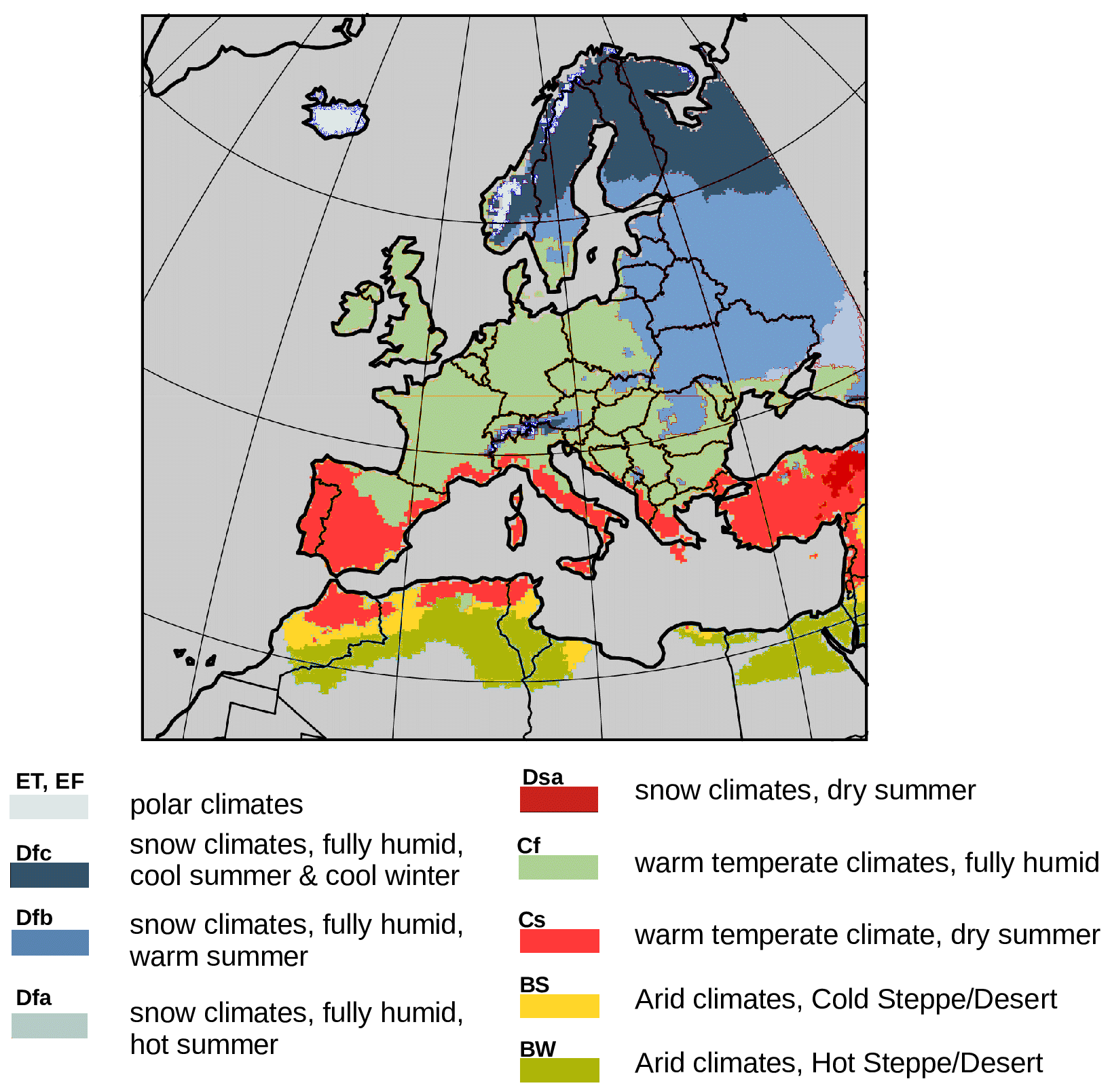
Figure 1Climate classification based on E-OBS monthly mean temperature and precipitation (Cornes et al., 2018). Classes are defined after Köppen (1923).
The Baltic Sea climate is influenced by a temperate, humid climate in the southwest and a snow climate in the north and east (Fig. 1), with an enhanced seasonal cycle giving rise to highly variable meteorological conditions related to predominant weather regimes over the region (Hertig and Jacobeit, 2014) ranging from severe storms, summer heat waves and winter cold-air outbreaks (Smith and Sheridan, 2020) to prolonged dry periods in the southern part. Many of these phenomena are directly subject to local and regional thermal feedbacks between the atmosphere, the land and the ocean and, thus, require a realistic exchange of mass and energy as realized by interactively coupled regional Earth system models.
1.2 Towards Earth system modeling of the Baltic Sea region
From a theoretical point of view, the coupling of two or more interacting models to create a more comprehensive system implies that boundary processes formerly prescribed, parameterized or even neglected are explicitly simulated. This removes observational constraints and/or empirically derived relationships on the model solutions and, thus, increases the model's degrees of freedom. Consequently, coupled models can drift from observed conditions; this makes their tuning more difficult but allows for a more realistic interaction between models. Therefore, in their hindcast modes, stand-alone models can be expected to be closer to observations once prescribed boundary conditions are of good quality.
From the climate perspective, which envisages simulations over several decades or even centuries, the model should ideally be drift-free to integrate over several million model time steps. Furthermore, with respect to future climate simulations, the model boundary conditions, such as temperature, are basically unknown and have to be derived from the output of available global climate models in the stand-alone case. Although advanced methods exist to make this data usable for high-resolution models (e.g., Hay et al., 2000; Chen et al., 2013), there is evidence that the solution of the ocean models is too tightly controlled by the global model in uncoupled ocean simulations (Mathis et al., 2018).
Hence, Earth system models are the prime tool for simulating cross-compartment feedback loops (Claussen, 2001; Giorgi and Gao, 2018; Heinze et al., 2019). In turn, such feedbacks play an important role in mediating the response of the Earth climate to a given external forcing or perturbation. Consequently, the ability of ESMs to simulate such feedbacks is essential. However, the capability of coupled models to better represent cross-compartment feedbacks and more realistically model dynamical processes is often not adequately accounted for during model validation. By contrast, model validation usually aims to demonstrate the models' ability to represent mean climate. By their nature, climate models are tools to iteratively solve the change in a variable from one given time step to the next rather than to predict the variable at a given time. From this, it follows that the capability of a model to reproduce transient behavior, such as interannual variability or long-term trends, is essential to estimate if a climate model can yield reliable answers to how changes in climate forcing will likely impact on climate variables. However, regional models are often validated more by how well they reproduce a given climatology of the present-day climate rather than by how well they reproduce trends derived from the historical past (Kerr, 2013). As every compartment model has its own spectrum of internal spatial scales and timescales, the inertia of the system increases when including slower components. This can become important, especially when a decision about the size of the ocean model domain has to be made. A larger extension to the open Atlantic or Arctic Ocean substantially increases the memory of the system, which has consequences for the model spin-up and the economical operation of the model system.
Over the past few decades, several advancements in coupled modeling have led to a growing number of different regional climate models on the way to a fully comprehensive description of the Earth system for many regions of the world, such as the east coast of the US (COAWST – Coupled Ocean–Atmosphere–Wave–Sediment Transport model; Warner et al., 2008, 2020). Recent reviews of global and regional Earth system modeling have elaborated past and recent trends and summarized future challenges for further development (Schrum, 2017; Giorgi and Gao, 2018; Giorgi 2019; Heinze et al., 2019; Jacob et al., 2020). Realized stepping stones on the road map towards coupled Earth system modeling for the Baltic Sea region include coupled ocean–sea-ice–atmosphere models, coupled ocean–wave and atmosphere–wave models, coupled vegetation–atmosphere models, and coupled ocean–atmosphere–hydrology models. This article aims at reviewing the latest developments, and describes the problems and benefits of using coupled models, with a focus on the specific demands of the Baltic Sea region within Europe. Thus, the emphasis is mainly set on the main physical feedbacks as they emerge in two-way coupled Earth system components. Therefore, this article does not aim to be comprehensive, as some important components are not considered, including biogeochemical nutrient cycling on land and in the Baltic Sea or atmospheric chemistry (e.g., the effect of aerosols).
2.1 Land surface–atmosphere coupling and modeling
2.1.1 Biophysical mechanisms
The Baltic Sea region's land surface and terrestrial ecosystems couple strongly to local climate, and biophysical interactions determine the exchanges of momentum, heat and water between the land and the atmosphere as well as the spatiotemporal dynamics of the atmospheric boundary layer (ABL), including the wind speed, surface and air temperature, humidity and precipitation, and the atmospheric radiative balance.
Changes in the properties of the land surface and ecosystems, whether natural or anthropogenic, will lead to climate change through a number of well-established biogeochemical and biophysical feedback mechanisms (IPCC 2019). The biogeochemical mechanisms include the release or uptake of greenhouse gases (primarily CO2, although CH4 and N2O are of considerable importance in the Baltic Sea region; Gao et al., 2014) and the emissions of black carbon, aerosol precursors (e.g., biogenic volatile organic compounds – BVOCs) and organic carbon aerosols that can alter the atmospheric composition, including cloud condensation nuclei and the fraction of diffuse and global radiation (e.g., Kulmala et al., 2014).
Important properties of the land surface include its albedo, its roughness, the species composition, the properties and phenology of green vegetation (e.g., leaf area index – LAI) and plant physiology (e.g., leaf stomatal and canopy conductance). Local climate is altered as a result of changes to the shortwave and longwave radiation, the turbulent fluxes of sensible and latent heat (i.e., evapotranspiration – ET) and momentum (e.g., Bonan 2008; Anderson et al., 2011; Pielke et al., 2011; Mahmood et al., 2014; Ellison et al., 2017; IPCC, 2019).
Forests typically have a lower surface albedo than grassland, pastures and cropland. Thus, deforestation tends to increase the albedo, whereas reforestation and afforestation have the opposite effect. Furthermore, coniferous forest albedo (0.05–0.15) is lower than deciduous forest albedo (0.15–0.20) (Anderson et al., 2011; Bonan 2008). Hence, the species composition determines the net albedo in a given region. As snow albedo ranges from 0.45 to 0.95 depending on age, history and mechanical disturbance, the albedo of the land surface in the Baltic Sea region is particularly sensitive to the duration and extent of snow cover as well as to the underlying vegetation type (Anderson et al., 2011). Reforestation or afforestation leads to a lower albedo in periods of snow cover, with greater net radiation at the land surface, stronger sensible heat fluxes and a warming over the forested area as a result (Anderson et al., 2011).
Since trees are taller than grasses and crops, forested regions in the Baltic Sea region have greater roughness lengths and tend to couple more strongly to the atmosphere, creating more turbulence than grass-covered regions or cropland, with higher sensible and latent heat fluxes. An increase in the surface roughness in association with reforestation or afforestation, increased rates of tree growth or altered forest management practices can lead to stronger turbulent fluxes and strong turbulent mixing (Winckler et al., 2019).
Trees transpire more water than grass or crops as a result of their larger leaf area and deeper roots. Thus, forests have higher evapotranspiration rates and latent heat fluxes than grasslands, although irrigated croplands can also have high ET rates. Higher latent heat fluxes cool the surface and moisten the ABL. A decrease in the latent heat fluxes associated with deforestation tends to warm the surface and leads to higher sensible heat fluxes and a warming of the ABL. The ABL is also drier, which can lead to a reduction in precipitation.
2.1.2 Biophysical effects of land-use and land-cover changes on climate in the Baltic Sea region
A number of modeling studies have examined the influence of land-use and land-cover change (LULCC) on climate variables in northern European domains, including the Baltic Sea region. The standard approach (Gálos et al., 2012; Strandberg et al., 2014; Strandberg and Kjellström, 2019) is to alter the static land-cover input to the coupled model and to compare simulations with an unchanged, control simulation. This approach does not permit two-way coupling in which local climate changes resulting from the perturbation subsequently alter land surface properties and vegetation characteristics.
Perugini et al. (2017; see also IPCC, 2019) reviewed the published literature on the biophysical effects of anthropogenic land-cover change on temperature and precipitation in boreal, temperate and tropical regions. A total of 28 studies were included in their review, including 3 based on observations and 25 that were based on idealized regional and global climate model simulations designed to estimate the regional and global biophysical effects of complete deforestation or afforestation. To effect deforestation in their simulations, some authors replaced forest with grassland, whereas other authors replaced forest with bare soil. Modeled deforestation in boreal regions resulted in local cooling consistent with observations but with a less consistent, slight cooling modeled in temperate regions in contrast to observations that indicate a slight warming in those zones.
Goa et al. (2014) used the REMO regional climate model (RCM) to investigate the biophysical effects of extensive peatland drainage and afforestation in Finland during the 20th century. Simulations were made for a model domain centered on Finland but covering a large part of the Baltic Sea region. The model grid had a horizontal resolution of 18 km with 27 vertical levels up to 25 km in the atmosphere.
Maps from the Finnish National Forest Inventory (FNFI) were used to compute changes to the fractional coverage of REMO's 10 land-cover classes in Finland from the 1920s, when peatland drainage and forestation began, to the 2000s. Over this period, coniferous forest replaced large regions previously covered by peat bogs and mixed forest. Two 18-year (1979–1996) simulations were then made to compare the effect of the land-cover change, driven with 6-hourly lateral boundary conditions from the ERA-Interim reanalysis data and identical land cover outside of Finland.
Goa et al. (2014) found that the reduction in albedo associated with prescribed peatland forestation resulted in an increase of up to 0.43 K in the 2 m air temperature in April, with the highest values being found over the most intensively forested areas. In contrast, there was a slight cooling (<0.1 K) during the growing season (May–October), associated with greater ET from coniferous forests.
Strandberg and Kjellström (2019) used the Rossby Centre RCM RCA4 (Strandberg et al., 2015; Kjellström et al., 2016), a successor to RCA3 (Samuelsson et al., 2011), to investigate and attribute the climate impacts of maximum potential afforestation or deforestation in Europe (see also the study by Gálos et al., 2012, using the REMO RCM). Horizontal grid spacing in RCA4 is approximately 50 km over the EURO-CORDEX domain covering Europe, and the model has 24 vertical levels in the atmosphere. For their study, Strandberg and Kjellström (2019) applied lateral boundary forcing (pressure, humidity, temperature and wind) every 6 h from ERA-Interim reanalysis data. Sea surface temperature and sea-ice extent were prescribed according to observations.
Three simulations, which only differed with respect to the land-cover map used, were performed for the 30-year period from 1981 to 2010. The control simulation used the standard, present-day land-cover map from RCA4 defined in the ECOCLIMAP (Champeaux et al., 2005) product. This map reflects the considerable agricultural activity in Europe, showing large areas with low forest cover in central, western and southern Europe. To effect maximum afforestation, Strandberg and Kjellström (2019) used the LPJ-GUESS dynamic vegetation model (Smith et al., 2001; see below) to produce a map of potential natural forest cover for Europe in equilibrium with present-day climate. Finally, maximum deforestation was implemented by converting forest fractions according to the potential forest cover to grassland in the control simulation.
In their analysis, Strandberg and Kjellström (2019) focused on winter (December–January–February, DJF) and summer (June–July–August, JJA) seasonal mean temperatures and precipitation as well as daily minimum and maximum temperatures. Afforestation decreased albedo in both seasons, especially in regions in eastern Europe with long snow cover and little forest cover. In contrast, deforestation increased albedo throughout the region, especially in the northern Baltic Sea region in winter.
Afforestation in Europe generally resulted in increased ET, as trees have a larger leaf area and deeper roots. This leads to colder near-surface temperatures in JJA. Deforestation gave the opposite effects, with warmer near-surface temperatures due to decreased ET in summer. In the Baltic Sea region, deforestation-induced reductions in ET coincide with the largest differences in the fraction of forest (e.g., a reduction of 20 %–35 % in Scandinavia). Interestingly, ET increases by 20 % over the Baltic Sea in JJA. Strandberg and Kjellström (2019) attribute this to a land–ocean coupling, whereby warmer and drier air from the surroundings (due to reduced ET over land) favors increased ET over the Baltic Sea when it comes into contact with the sea.
Afforestation in winter resulted in a decrease in temperature in central and southern Europe that can not be explained by albedo changes, as this is reduced during these months. As ET is also low during winter, the changes were attributed to atmospheric circulation changes resulting from increased roughness.
The winter low-pressure systems simulated by RCA4 lose their energy earlier because of increased friction over afforested areas due to their greater roughness, and afforestation generally leads to a simulated winter climate with less cyclonic activity in central Europe. Associated with this, the mean geopotential height at 500 hPa increased by 100 m in the Baltic Sea region.
Strandberg and Kjellström (2019) also found that the biophysical effects of afforestation or deforestation in Europe on daily minimum and maximum temperatures were stronger than the impacts on mean near-surface temperatures. In the case of afforestation, although DJF mean temperatures were reduced throughout most of Europe, there was a particularly strong warming of daily minimum temperatures (up to 2–6 ∘C in Germany) that could be attributed to increased cloud cover and reductions in outgoing longwave radiation. During summer, on the other hand, the marked changes in mean temperatures were mainly caused by respective changes in daily maximum temperatures (i.e., decreases in the case of afforestation and increases in the case of deforestation). Finally, by rerunning the simulations and confining the applied deforestation and afforestation changes to the western and/or eastern parts of the model domain, the authors also showed that the climatic effects of afforestation or deforestation in Europe were mainly local.
Belušić et al. (2019) followed up on the study of Strandberg and Kjellström (2019) and used a cyclone-tracking algorithm to study how the same idealized deforestation and afforestation scenarios affected the number and intensity of cyclones as well as how they affected precipitation extremes. Consistent with the results of Strandberg and Kjellström (2019), Belušić et al. (2019) found that the larger surface roughness after afforestation reduced the number of cyclones over Europe compared with the deforestation and control simulations: differences were 20 %–80 % near the Baltic Sea region, 10 % in regions near the western European coast and they increased towards the east to reach 80 %. This resulted in a reduction in winter precipitation extremes of up to 25 % across the domain.
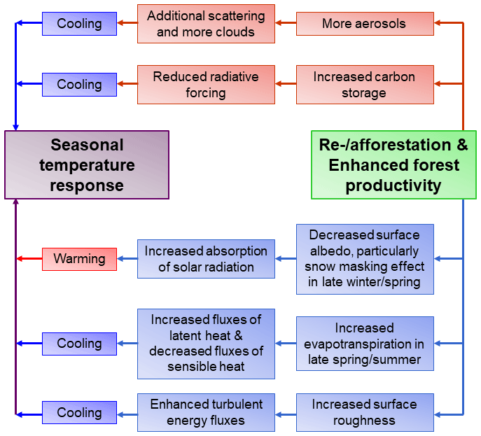
Figure 2Outline of the biogeochemical (upper part in brown) and the biophysical (lower part in blue) influence of reforestation/afforestation or enhanced forest productivity in the Baltic Sea region on near-surface temperatures. The overall effect on near-surface temperatures varies by season and region, depending, for instance, on snow cover and incoming solar radiation (adapted from May et al., 2020).
Figure 2 summarizes the various biophysical and biogeochemical influences of reforestation and afforestation or enhanced forest productivity on near-surface temperatures in the Baltic Sea region. According to the figure, the decrease in surface albedo (resulting in increased absorption of incoming solar radiation at the land surface) is the only effect that leads to a warming of near-surface temperatures, while all the other effects lead to a cooling. The biogeochemical effects shown in Fig. 2 are increased carbon (C) storage, which weakens the radiative forcing, and more aerosols, which reduce the solar radiation reaching the land surface due to additional scattering from particles and more clouds. The biophysical effects shown are increased roughness length, which enhances the turbulent fluxes of energy and momentum, and increased evapotranspiration in late spring and summer, which strengthens the fluxes of latent heat and weakens the fluxes of sensible heat. The magnitude of the overall cooling in the Baltic Sea region associated with reforestation and afforestation or enhanced forest productivity depends on the significance of the warming effect compared with the cooling from the other biophysical and biogeochemical effects.
Following up on their earlier, theoretical and observation-based studies in which changes in land management were shown to affect surface temperature to a degree similar to changes in land-cover type (Luyssaert et al., 2014), Luyssaert et al. (2018) used the ORCHIDEE-CAN land surface model (further developed to explicitly take the biogeochemical and biophysical effects of land-use change and management into account) coupled to the LMDZ atmospheric circulation model to investigate the trade-offs associated with using European forests to meet the climate objectives of the Paris Agreement. Their analyses clearly demonstrate that the biophysical effects of forest management must be taken into account in any assessment of climate mitigation strategies, with consequences for policy and forestry in the Baltic Sea region and beyond (e.g., in relation to the optimal balance of coniferous and deciduous forest in the region). Similarly, Kumkar et al. (2020) used offline simulations with the CLM4.5 land surface model to quantify the sensitivity of turbulent fluxes and land surface temperatures in Fennoscandia to scenarios of changes to forest composition and structure relative to their present-day values. They found that replacing conifers with deciduous forests could cool the surface by 0.16 K annually and by 0.3 K is summer months, mainly as a result of their higher albedo, and they identified important differences between developed and underdeveloped forests, with the latter having lower evaporation rates as a result of their lower LAI and canopy height.
2.1.3 Dynamic global vegetation models applied to the Baltic Sea region
Dynamic global vegetation models (DGVMs) are numerical models of terrestrial ecosystems that simulate the properties, dynamics and functioning of potential, natural and managed vegetation and their associated biogeochemical and hydrological cycles as a response to climate and environmental change. Prentice et al. (2007) summarize their historical development, design and construction principles as well as the processes typically included, their evaluation and examples of their application. DGVMs incorporate research and knowledge from different disciplines, including plant geography; plant physiography; biogeochemistry, including soil biogeochemistry; vegetation dynamics and demography; biophysics; agriculture; and forest management. DGVMs have been used to study the observed and expected impacts on terrestrial ecosystems in the Baltic Sea region resulting from climate and environmental change. An understanding of these impacts is a necessary first step to comprehending the dynamics in coupled RESMs, where ecosystem change is allowed to influence local and regional climate through the biophysical feedback mechanisms outlined above.
Recent works have shown that in order to realistically simulate ecosystem carbon balance, climate responses, and ecosystem recovery following disturbances due to land-use change, management interventions, and natural disturbance processes such as fires and storms (Fisher et al., 2018; Pugh et al., 2019), it is important to incorporate the size- and age-structure and demography of vegetation and ecosystems explicitly, and to account for the competitive interactions of growing vegetation stands comprising individuals or cohorts of different plant functional types. A number of DGVMs and land surface models (LSMs) are now moving in this direction, away from a traditional tiled or area-based (Smith et al., 2001) land surface representation, including the CLM4.5(ED) LSM (Moorcroft et al., 2001; Fisher et al., 2015, 2018) and the Functionally Assembled Terrestrial Ecosystem Simulator (FATES) vegetation demography submodel (Koven et al., 2020), the POP (Population Orders Physiology) module for woody demography in the CABLE LSM (Haverd et al., 2013, 2014, 2018), the RED module in the JULES LSM (Argles et al., 2020) and the SEIB-DGVM (Sato et al., 2007). To date, however, no demographic model has been applied to study the Baltic Sea region specifically (see Kumkar et al., 2020, for an application using CLM4.5) apart from the LPJ-GUESS DGVM (Smith et al., 2001, 2014). LPJ-GUESS explicitly represents the size, age structure, spatial heterogeneity and temporal dynamics of co-occurring cohorts of plant functional types (PFTs), i.e., classifications of plants according to their physical, phylogenetic and phenological characteristics (e.g., boreal or temperate, evergreen or deciduous, and broadleaf or needleleaf trees in the Baltic Sea region, and herbaceous species; Prentice et al., 2007) or species (Hickler et al., 2012) that compete in natural and managed stands (forestry, crops and pasture), in response to climate, atmospheric CO2 and nitrogen (N) availability. As the stand structure evolves in response to environmental change and impacts the availability of key resources, the growth, survival and the outcome of competition are affected.
LPJ-GUESS represents different land use and management in separate stands (Lindeskog et al., 2013). The fraction of the grid cell covered by each stand (e.g., forest, natural and cropland) type can change in time, following external land-use datasets (e.g., Hurtt et al., 2020). LPJ-GUESS also allows for detailed management interventions for representative crops (represented as crop functional types – CFTs), grassland grazing, mowing and fertilization (Olin et al., 2015a, b) as well as clear-cut and continuous-cover forest management (Lagergren and Jönsson, 2017). Disturbances due to management actions such as forest clearing, prognostic wildfires and a stochastic generic disturbance regime induce biomass loss and reset vegetation succession (Smith et al., 2001). N-cycle-induced limitations on natural vegetation and crop growth, C–N dynamics in soil biogeochemistry and N trace gas emissions are included (e.g., Smith et al., 2014; Olin et al., 2015a, b) as well as BVOC (isoprene and monoterpene) emissions (Hantson et al., 2017).
LPJ-GUESS output variables describe the vegetation state (PFT/species composition, LAI, vegetation height, biomass, tree density, and burned area), variables relating to the state and functioning of the soil (water content, C and N content, temperature, runoff, N leaching, and loss of dissolved organic C and N), and climatically important fluxes to and from each simulated stand (evapotranspiration, gross and net primary productivity, autotrophic and heterotrophic respiration, fluxes from wildfires, CH4 and N trace gases, BVOCs, and net ecosystem carbon exchange).
2.1.4 Modeling terrestrial ecosystems in the Baltic Sea region
LPJ-GUESS has been applied in many studies to simulate terrestrial ecosystems in the Baltic Sea region, under current, future, and historic and preindustrial climate conditions. Koca et al. (2006) simulated the impacts of climate change on natural ecosystems in Sweden in response to different regional climate change scenarios. In all of the climate scenarios considered, the authors observed an increase in plant productivity and LAI, and a northward and upward advance of the boreal forest tree line by the end of the 21st century. The current dominance of Norway spruce and to a lesser extent Scots pine was found to be reduced in favor of deciduous broadleaf tree species in future scenarios across the boreal and boreo-nemoral zones. These changes are consistent with earlier studies (Miller et al., 2008) of the effects of climate and biotic drivers on Holocene vegetation in Sweden and Finland, where observed changes to the northern distribution limits of temperate trees and species at the tree line were attributed to millennial variations in summer and winter temperatures.
Hickler et al. (2012) reparameterized the most common European tree species in LPJ-GUESS and forced the model with an atmosphere–ocean general circulation model (AOGCM) climate scenario output, downscaled to a spatial resolution of 10 arcmin×10 arcmin. Climate change and CO2 increase resulted in large-scale successional shifts, with 31 %–42 % of the total area of Europe projected to be covered by a different vegetation type by the year 2085 depending on the scenario used. Consistent with the earlier results of Koca et al. (2006), trees replace tundra in arctic and alpine ecosystems, and temperate broadleaf forest replaces boreal conifer forest in the Baltic Sea region.
2.1.5 Regional Earth system modeling with interactive vegetation dynamics in the Baltic Sea region
Coupled regional Earth system models (RESMs) extend RCMs to include the terrestrial biosphere as an integral dynamic component interacting in a two-way coupling with the atmosphere, with representations of both vegetation dynamics and terrestrial biogeochemistry. Such a framework allows for modeled natural and managed ecosystems to respond to climate and environmental change and to influence local and regional climate through the biophysical feedback mechanisms outlined above.
RCA-GUESS was the first published and evaluated RESM (Smith et al., 2011) to include the terrestrial biosphere as an integral dynamic component, and it couples LPJ-GUESS to the RCA3 RCM (Samuelsson et al., 2011). In its RCA-GUESS configuration, LPJ-GUESS is driven by the daily mean temperature, soil water content, precipitation and downward shortwave radiation simulated by RCA3, and the CO2 concentration is read from the same source used to force RCA.
In its uncoupled configuration, the land surface scheme of RCA3 uses ECOCLIMAP to specify the cover fractions of two vegetated land surface tiles, one representing the type of forest (broadleaf or needleleaf) and the other open land (including crops, pasture and grassland) for each grid cell in its domain.
In RCA-GUESS, LPJ-GUESS replaces the static ECOCLIMAP land-cover description and aggregates its vegetation fields to update the tile fractions, their type and their associated LAI. The specific forest PFTs simulated by LPJ-GUESS are aggregated into needleleaf and broadleaf trees before providing the information to RCA, while open land includes a varying coverage of herbaceous vegetation.
By changing the relative fractions and types in RCA, the LPJ-GUESS fields dynamically determine and update the surface albedo, LAI, surface roughness and conductance in RCA grid cells. For example, albedo is calculated in RCA using a weighted average of prescribed albedo values for needle leaved and broadleaf trees, open land vegetation, snow and bare soil. Similarly, the fluxes of sensible and latent heat are calculated as weighted averages of the individual tiles.
Terrestrial CO2 exchange is simulated by LPJ-GUESS, enabling biogeochemical ecosystem responses to be assessed consistently with the biophysical land–atmosphere interactions (Zhang et al., 2014). However, the atmospheric CO2 concentrations are not updated over the limited domain covered by RCA. Thus, although biophysical feedback loops are closed in RCA-GUESS, biogeochemical feedback loops are open.
Wramneby et al. (2010) used RCA-GUESS to identify hot spots of biophysical vegetation–climate feedbacks for future climate conditions in Europe. Two simulations – feedback and non-feedback – were run over Europe for 1961–2100 to isolate the effect of feedbacks from vegetation dynamics. In the feedback simulation, RCA and LPJ-GUESS were coupled throughout the entire simulation period. In the non-feedback simulation, land cover in RCA was prescribed and fixed over the full simulation period from the long-term means from LPJ-GUESS output in the coupled simulation for 1961–1990. The difference between the climate change signal (2071–2100 minus 1961–1990) from the feedback simulation and the corresponding signal from the non-feedback simulation was used to calculate the additional contribution of the vegetation–climate feedback to the background climate changes simulated by RCA3, driven by lateral AOGCM forcing.
Wramneby et al. (2010) showed that the snow-masking effect of forest expansion and greater LAI in the Scandinavian mountains as well as the consequent reductions in albedo enhanced the winter warming trend. In central Europe, the stimulation of photosynthesis and plant growth caused by the increased CO2 concentration, longer growing seasons and warming mitigated the future warming through a negative feedback due to enhanced ET associated with the increased vegetation cover and LAI.
Zhang et al. (2014, 2018) applied RCA-GUESS over the Arctic domain of the Coordinated Regional Climate Downscaling Experiment (CORDEX-Arctic) – which includes the northern part of Baltic Sea region – to investigate the role of the biophysical feedbacks from vegetation in the Arctic region under three different climate scenarios (RCP2.6, RCP4.5 and RCP8.5, where RCP stands for Representative Concentration Pathway). Zhang et al. (2018) found that warming and CO2 increases promote productivity increases, LAI increases and tree line advance into the Arctic tundra, with the consequence that two biophysical effects have the potential to alter the spatiotemporal signal of future climate change in the Arctic region: interactive vegetation results in albedo-mediated warming in early spring and ET-mediated cooling in summer, amplifying or modulating local warming and enhancing summer precipitation over land.
2.2 Ocean–atmosphere coupling
The treatment of ocean–atmosphere exchange of momentum, heat and mass substantially differs between coupled and uncoupled models. Basically, in the coupled mode, the ocean is driven by fluxes and sea level pressure calculated in the atmosphere model (e.g., Fig. 3) and is used to drive the coupled ocean model which, in turn, communicates simulated fields of sea ice and surface water temperature (SST) to the atmosphere model. By contrast, uncoupled ocean models use atmospheric forcing fields (passively coupled ocean, PCO) to calculate air–sea fluxes with a bulk formula. Stand-alone atmosphere models usually read prescribed fields of sea ice and SST from reanalysis datasets or model data to calculate fluxes.

Figure 3Mass, momentum and heat exchange as realized in the atmosphere–ocean model RCA4-NEMO. The abbreviations used in the figure are as follows: ICA – interactively coupled atmosphere, PCA – passively coupled atmosphere, ICO – interactively coupled ocean and PCO – passively coupled ocean. Source: Gröger et al. (2015).
2.2.1 Impact on mean climate
One of the main questions addressed so far is if an interactively coupled atmosphere–ocean model would significantly change the long-term climate compared with their stand-alone atmosphere and ocean modules. This has been investigated in a number of studies (e.g., van Pham et al., 2014; Tian et al., 2013; Gröger et al., 2015, 2021; Primo et al., 2019; Kelemen et al., 2019; Akhtar et al., 2019; Cabos et al., 2020). Van Pham et al. (2014) developed a regional atmosphere–ocean general circulation model (RAOGCM) built upon the ocean model NEMO coupled to the atmosphere model COSMO-CLM (the COSMO model in Climate Mode, hereafter denoted as CCLM) for the EURO-CORDEX domain. The coupling domain encompassed the Baltic Sea and the North Sea until 59∘ N and 4∘ W. As forcing as well as at the lateral model boundaries, the authors applied ERA-Interim reanalysis data. It is noteworthy that the coupled system showed a systematically lower long-term mean 2 m air temperature (T2m) in the Baltic Sea and North Sea compared with the uncoupled atmosphere model. Consequently, interactive coupling reduced the model's mean bias in T2m compared with the E-OBS observational dataset as a reference. Interestingly, the authors found most significant changes between coupled and uncoupled runs over continental areas of central and eastern Europe (i.e., at a distance from the coupled areas). Analysis of the modeled wind field indicated that these areas were situated downwind from the coupled domain in the North Sea and Baltic Sea, implying a more complex pattern of atmospheric advection of temperature anomalies which was not further investigated.
However, similar experiments by Gröger et al. (2015), using nearly the same ocean model NEMO but coupled to the regional atmosphere model RCA4, were somewhat contradictory. In their setup forced by ERA40 reanalysis data with lateral boundaries prescribed by ORAS4 (Balsameda et al., 2013), the coupled system showed generally warmer near-surface air temperatures over the Baltic Sea compared with the uncoupled RCA4 model. Furthermore, no significant differences were found in air temperatures over land between coupled and uncoupled simulations. With respect to sea surface temperatures, Gröger et al. (2015) found the strongest differences in the Baltic Sea, where SSTs in both the coupled and uncoupled system were too cold in winter compared with satellite products. However, winter SSTs were significantly higher in the coupled model (thereby reducing the bias) due to seasonally varying feedback loops controlling the ocean–atmosphere heat exchange. Figure 4 sketches the main mechanisms comprising the atmosphere–ocean feedbacks during summer and winter that control the SST in the Baltic Sea.
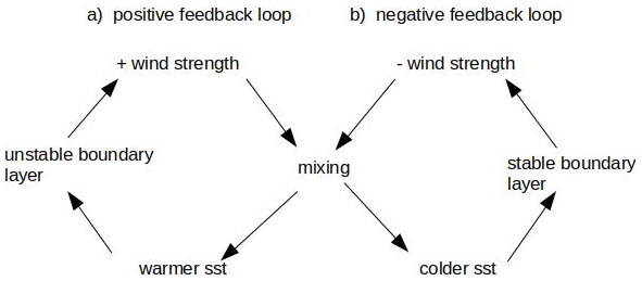
Figure 4Side (a) of the figure shows a positive winter feedback loop, and side (b) shows a negative summer short-circuit. Drawn after Gröger et al. (2015).
Winter thermal–wind mixing positive feedback
During winter, the Baltic Sea is usually warmer than the atmosphere, supporting a net heat flux out of the ocean.
During ocean offline simulations, in which the ocean model was forced with ERA40 atmospheric reanalysis data, simulated winter SSTs in the Baltic Sea showed a strong bias compared with observed SSTs. This was mainly caused by a cold bias of the ERA40 dataset over Europe. In the coupled mode and driven by the same dataset at the lateral boundaries, the bias nearly vanished due to a thermal feedback loop between the ocean and the atmosphere which resulted in stronger vertical mixing and increased transport of warmer deep waters to the surface (thereby reducing the cold bias at the surface compared with the uncoupled simulation). This is shown in Fig. 4a. In the coupled model, the atmospheric boundary layer is disturbed by warm anomalies generated in the Baltic Sea. This promotes stronger winds that, in turn, feed back to the ocean with stronger vertical mixing, thereby increasing heat exchange with warmer, deeper water layers. As a result, the ocean model's cold bias decreases in the Baltic Sea compared with the ocean stand-alone model which uses prescribed atmospheric boundary conditions that can not respond to SST anomalies (Gröger et al., 2015).
Summer thermal short-circuit
During summer, the above feedback loop is bypassed by the inverse thermal air–sea contrast. As the atmosphere is generally warmer than the ocean in summer, any wind-induced upward mixing of cold, deep water will tend to stabilize the atmospheric boundary layer with a negative effect on wind strength (Fig. 4b). This was demonstrated at stations in stratified areas of the Baltic Sea and in the North Sea using lead correlation analysis between the 10 m wind velocity and SST after a short-term event of strengthened winds (Gröger et. al., 2015). During the first 70 h after the event, the wind and SST were negatively correlated (with a peak r=0.7 at around 30 h), implying decreasing SST with stronger wind mixing with colder deep waters. After 70 h, the correlation turned to positive values with a peak (r=0.7) around 130 h as the colder water surface stabilized the atmospheric boundary layer and, thus, promoted lower wind speeds. Following this, wind mixing ceased again giving rise to heat gain from the warmer atmosphere Gröger et al. (2015).
These results highlight the importance of thermal air–sea coupling in midlatitude marginal seas and are supported by a number of different studies. Tian et al. (2013) drove a coupled ocean–atmosphere model with ERA-Interim reanalysis data (ERA-I). Similar to Gröger et al. (2015), the abovementioned authors also found overly cold SSTs in winter but with a substantial lower bias in the coupled model. No detailed feedback analysis was carried out, but it is likely that the positive winter feedback was also present in the model of Tian et al. (2013). Moreover, Keleman et al. (2019) applied a model that couples an atmosphere model for the EURO-CORDEX region to regional ocean models for the Mediterranean, the North Sea and the Baltic Sea. They found a significant improvement in winter precipitation patterns over eastern Europe through the altered representation of SSTs. However, the SSTs themselves were not validated; thus, a general conclusion on the performance of the whole system can not be drawn. Primo et al. (2019) used the same model and showed that air–sea coupling can improve the representation of heat and cold waves but concluded that a general judgment regarding the whole system is difficult to draw and depends on the variable considered.
Impact on climate indices
Apart from the thermal coupling effect on mean climate, we now consider temperature-related climate indices often used in regional climate assessments such as CORDEX (e.g., Jacob et al., 2014; Teichmann et al., 2018; Kjellström et al., 2018; Gröger et al., 2021). The indices are strongly related to the ocean heat content and are, therefore, sensitive to the coupling. In particular, we focus on three indices with importance for human health, agriculture and the Baltic Sea ecosystem: (1) the number of tropical nights, which are defined as nights when the daily minimum temperature does not fall below 20 ∘C (e.g., Fischer and Schär, 2010; Teichmann et al., 2018; Meier et al., 2019a; Gröger et al., 2021); (2) the number of frost days, which are defined as days when the daily minimum temperature falls below 0 ∘C; and (3) the number of warm periods, defined as at least 3 consecutive days on which the daily maximum temperature reaches 20 ∘C. For our analysis, we take available data from hindcast runs, as described in Gröger et al. (2015). All indices are derived from the 1970–1999 reference period from both the coupled and the uncoupled simulations. Both runs are driven with ERA40 atmospheric reanalysis data at the lateral model domain boundaries. Lateral boundary conditions were set according to the ocean reanalysis ORAS4 (Balsameda et al., 2013). For details about the coupling, we refer the reader to Gröger et al. (2015) and Dieterich et al. (2019b).
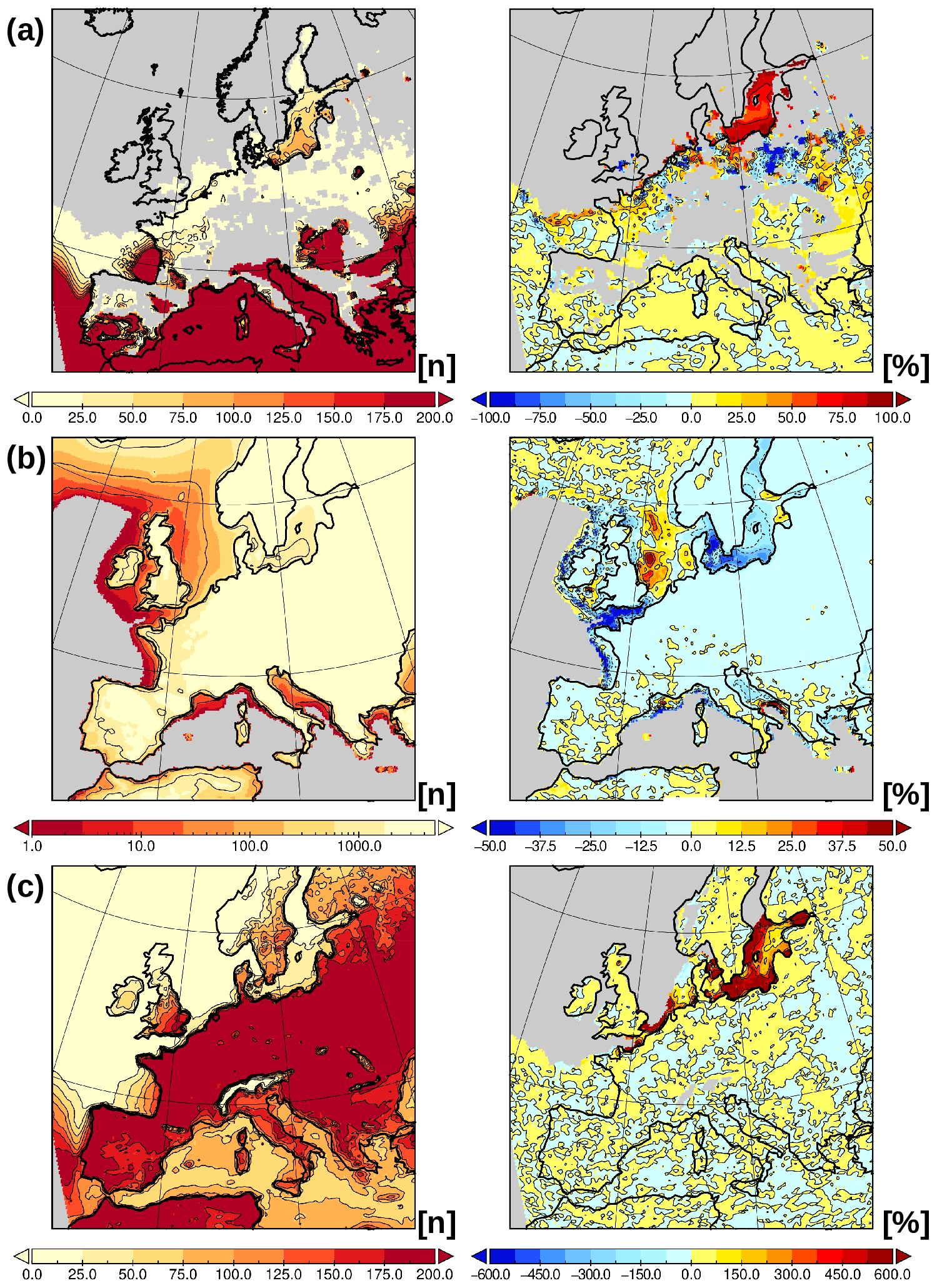
Figure 5The left panel of (a) shows the number of tropical nights diagnosed from the coupled regional ocean–atmosphere model during the 1970–1999 reference period. The right panel of (a) displays the difference (%) of the coupled minus the uncoupled model. The panels in (b) are the same as those in (a) but for the number of frost days. The left panel of (c) shows the number of periods of at least 3 consecutive warm days (days when the daily maximum temperature exceeds 20 ∘C). The right panel of (c) displays the difference (%) of the coupled minus the uncoupled model.
Figure 5a displays the number of tropical nights simulated with the coupled ocean–atmosphere model RCA4-NEMO (Wang et al., 2015; Dieterich et al., 2019b; Gröger et al., 2019, 2021). A clear land–sea pattern is seen with only sporadic occurrences over land with the exception of the southern part of the Iberian Peninsula and the Pannonian Basin south of the Carpathians. The higher effective heat capacity of the ocean is responsible for the frequent occurrences over the Mediterranean and over the southern North Atlantic sector, which also includes the Bay of Biscay. The thermal effect of the Baltic Sea water body is obvious. Unlike the North Sea, which receives colder waters from the North Atlantic, the Baltic Sea has very limited exchange of waters with the adjacent North Sea. In addition, a strong seasonal thermocline during summer also limits the exchange with colder waters from deeper layers. These two processes support a strong warming of the Baltic Sea during summer. Consequently, this prevents the air temperature from falling below 20 ∘C during warm periods in the second half of the summer. As a result, the Baltic Sea displays a range of tropical nights that matches the range found further to the south, such as north of the Black Sea or in parts of the western Atlantic off northern Iberia (Fig. 5a, left). Figure 5a (right) demonstrates that the abovementioned thermal effect over the Baltic Sea is much more pronounced in the coupled model including the dynamic ocean model. As a result, the number of detected tropical nights within the reference period increases by between 50 % and 100 % over the southern Baltic Sea in the coupled model compared with the stand-alone atmosphere model.
Figure 5b (left) shows the number of frost days during the reference period. A clear land–sea pattern is seen with strongly diminished occurrences over the open-ocean areas in the north, whereas they are completely absent over the southern Mediterranean and the southern part of the Atlantic. Again, the different thermal behavior between the North Sea and the Baltic Sea is obvious. With respect to its thermal behavior, the Baltic Sea is similar to the continents and supports a large number of frost days. This is related to the strong winter halocline that hampers wind-forced mixing and convective mixing with deep waters. Consequently, the upper-layer water body of the Baltic Sea can rapidly cool during winter. In contrast, the adjacent North Sea effectively damps the occurrence of frost days. However, a pronounced east–west gradient is visible with fewer occurrences in the west. Here, warmer waters from the Atlantic enter the North Sea and spread southward. The eastern part of the North Sea is influenced by low-salinity waters derived from the Baltic Sea. These waters flow northward along the Norwegian coast and impose a haline stratification there. This results in similar thermal behavior to that discussed for the Baltic Sea. The southern part of the eastern North Sea, namely the German Bight, is shallow and supports rapid cooling. Altogether, this creates the east–west gradient seen in Fig. 5b (left). Generally, these thermally forced processes are represented in both the coupled and uncoupled model versions, but in the coupled model, the number of frost days is significantly decreased over almost the entire Baltic Sea (Fig. 5b, right). Here, the aforementioned winter mixing feedback loop operates (i.e., stronger mixing in the coupled model increases the winter sea surface temperature with a positive feedback on wind speed, resulting in a significantly higher sea surface temperature and reducing the number of frost days). Over the North Sea, coupling generates a positive anomaly along a band between the 2–4∘ E meridian. It is likely that this reflects shifts in the gradients caused by slightly altered flow paths of the water masses derived from the Baltic Sea and the North Sea.
Finally, the coupling effect of warm periods is displayed in Fig. 5c. In the Baltic Sea, such periods are an important precondition for the occurrence of cyanobacteria blooms during summer. Moreover, the southern Baltic Sea is found be a hot spot with respect to the effect of interactive air–sea thermal coupling, as the number of such periods in the coupled model exceeds the corresponding number in the stand-alone atmosphere model by several orders of magnitude. Here, the effect of the aforementioned summer thermal short-circuit is seen. Enhanced mixing by winds brings cooler waters from the depths to the surface. The cooler surface water also lowers the air temperatures; this imposes a stabilizing effect on the atmospheric boundary layer over sea, thereby further damping wind strength (see Gröger et al., 2015, for details). This facilitates the development of longer-lasting warm periods in summer.
So far, we have discussed the thermal effects of damping (in the case of frost days) and amplifying (warm days and tropical nights). The associated feedback loops are more realistically represented in the fully coupled model, as previously explained. However, effects outside of the active coupling area over land seem to be rather weak. On the other hand, we note that the interactive coupling area must be considered small compared with the whole domain. Thus, extending the area of interactive coupling by, for example, also including the Mediterranean or larger parts of the North Atlantic may result in more intense effects when using coupled models (Primo et al., 2019; Keleman et al., 2019; Akhtar et al., 2019; Cabos et al., 2020).
2.2.2 Impact on extreme events
Apart from the representation of mean climate, many air–sea coupling processes are important in generating hazardous events such as extreme precipitation, storm track paths or flooding (see also Rutgersson et al., 2021). Often these events are generated remotely over the open ocean and, thus, require a realistic representation of the ocean's surface. Therefore, when no high-resolution ocean model is coupled to the regional atmosphere model, the sea surface has to be represented by available products for sea surface temperatures (SSTs) and sea ice. These products are often limited in quality and frequency. For example, the ERA40 SSTs, which are often used in uncoupled atmosphere simulations, are based on a weekly or even monthly frequency (Fiorino, 2004; Uppala et al., 2005). Consequently, many studies have compared coupled and uncoupled models with respect to the representation of extreme events in hindcast simulation. More recent products such as ERA5 may improve the situation by providing higher spatial and temporal resolution data.
Jeworrek et al. (2017) diagnosed a better representation of atmospheric conditions favorable for the occurrence of convective snow bands. The authors attributed this improvement to a more accurate simulation of SSTs and subsequent air–sea heat and moisture fluxes in a case where the atmosphere model RCA4 was coupled to the ocean model NEMO setup for the North Sea and Baltic Sea. The importance of accurate SSTs for the representation of snow bands was recognized early by Gustafsson et al. (1998).
Comparing two regional ocean–atmosphere models in coupled and uncoupled mode, Ho-Hagemann (2015, 2017) found that interactive air–sea coupling can alter extreme precipitation over land. The abovementioned authors pointed out that the coupled model COSTRICE improved the low-level large-scale moisture convergence over the North Atlantic and the moisture transport towards central Europe. As a result, the simulated summer heavy rainfall improved compared with the stand-alone atmospheric model CCLM. This was demonstrated for several flood events in central Europe. A diagram displaying the cause and effects as well as feedbacks between the Earth system components is shown in Fig. 6 in order to explain the physical mechanism behind the improved representation of heavy rainfall. The main effect is an altered SST in the coupled model which further influences wind speed and evaporation – the so called wind–evaporation–SST (WES) feedback (Xie and Philander, 1994). When the wind speed increases over an area, evaporation increases and the latent heat flux is subsequently enhanced, which often leads to ocean cooling over the area in question. The lowered SST generates a horizontal SST gradient on the sea surface and also increases the land–sea heat contrast which, in turn, supports increasing wind speed. Stronger wind over the North Sea then generates a larger latent heat flux from the ocean to the atmosphere and intensifies the low over central Europe and the North Sea, which both support the large-scale moisture convergence from the North Sea to central Europe. A review of the influence of atmosphere–ocean interactions on heavy rainfall over Europe is available in Ho-Hagemann and Rockel (2018).
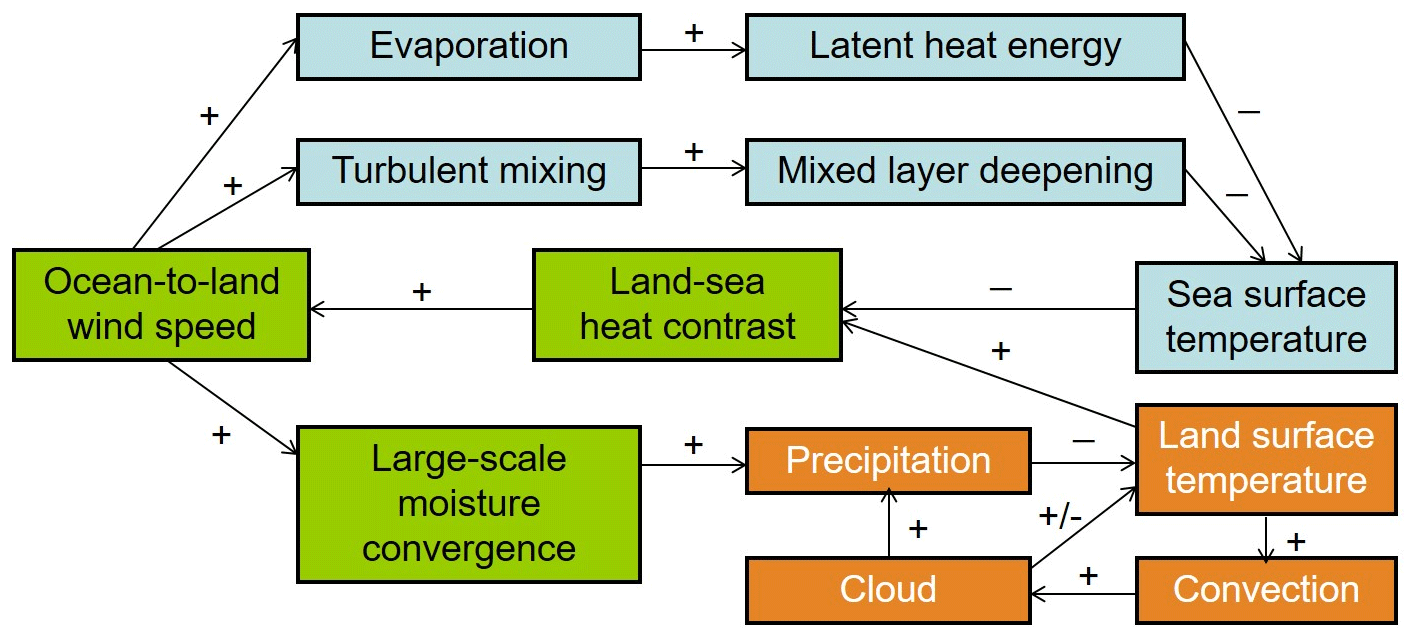
Figure 6An air–sea feedback and interaction diagram. For each arrow, the initial status indicates that the source quantity is increasing, and the sign (− or +) indicates the changing tendency of the target quantity. Colors denote the group of changes or states over sea (blue), land (brown) and the land–sea interactions (green). Source: Ho-Hagemann et al. (2017).
An improved representation of extreme and mean temperatures in the CCLM atmosphere models is also reported in Primo et al. (2019) and Kelemen et al. (2019) when coupled to regional high-resolution ocean models for the North Sea, the Baltic Sea and the Mediterranean. Akhtar et al. (2014) analyzed 11 historical medicane events simulated by the atmosphere-only model CCLM and the coupled model CCLM-NEMOMED12 with different horizontal atmospheric grid spacings of 0.44, 0.22 and 0.08∘. In this analysis, the coupled simulations improved significantly compared with atmosphere-only simulations at higher atmospheric grid resolution (0.08). The characteristic features of medicanes, such as warm cores and high wind speeds, are more intense in coupled simulations compared with atmosphere-only simulations. Akhtar et al. (2019) also demonstrated improved simulations of cyclones over the Mediterranean in the coupled system model of CCLM and two ocean models, NEMO-Nordic and NEMOMED12, compared with the atmosphere-only model with prescribed SSTs.
The impact of air–sea coupling on simulations of midlatitude cyclones was recently investigated by Ho-Hagemann et al. (2020) using an ensemble approach. The coupled model GCOAST-AHOI reduces the large spread of wind speed, mean sea level pressure, surface temperature, cloud cover and radiation fluxes amongst ensemble members of the atmospheric model during Cyclone Christian, which occurred in northern Europe between 27 and 29 October 2013.
2.2.3 Influence of the size of the coupling area
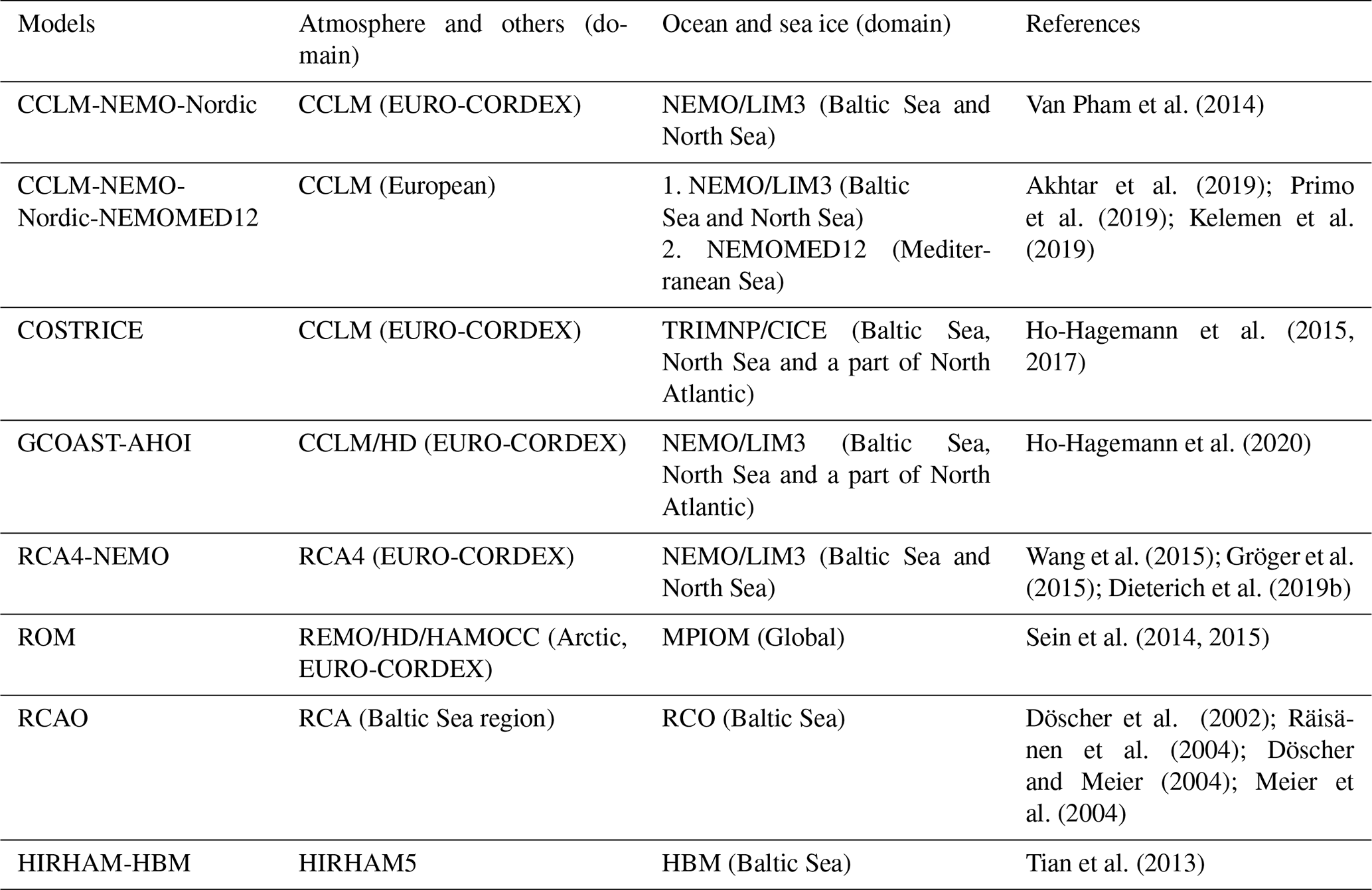
As outlined above, the size of the air–sea coupling area will influence how strong the coupling effect will be and how far it may propagate further over land. Table 1 lists several RAOGCMs applied for the Baltic region that have been developed for various areas within the recent decade. In these regional coupled system models (RCSMs), the atmospheric models cover different domains, such as the EURO-CORDEX domain, the European domain or the Arctic. The domain of the ocean model can be global with increased resolution over the North Sea and Baltic Sea as in MPIOM (Sein et al., 2015), or regional as in the other RCSM setups. For example, in a common NEMO setup used by several RAOGCMs (e.g., Van Pham et al., 2014; Gröger et al., 2015; Wang et al., 2015; Dieterich et al., 2019b; Akhtar et al., 2019; Primo et al., 2019), the Baltic Sea and North Sea regions are considered. In other coupled systems, such as Ho-Hagemann et al. (2015, 2017, 2020), the ocean model domain extends from the Baltic Sea and North Sea region into a part of the North Atlantic. Moreover, one atmospheric model can be coupled to more than one ocean model as in Akhtar et al. (2019) and Primo et al. (2019).
Table 1Regional coupled climate models and their air–sea coupling domains.
A recent assessment of regional coupled modeling (Schrum, 2017) emphasized that the location and extension of the coupled region (Sein et al., 2014), the coupling frequency (Fang et al., 2009), and the quality of initialization and boundary forcing (Wei et al., 2014) are critical. In the following, we focus on the size of the coupling area and consider its potential impact on climate simulations. We will also elaborate on options with respect to suitable sizes for the coupling area.
Sein et al. (2014) pointed out that the choice of the coupled model domain based on simple geographical arguments is not sufficient, and decisions should be made based on the fundamental understanding of oceanographic and atmospheric processes and their feedbacks. Mikolajewicz et al. (2005) discussed the challenges regarding the global mass and energy balance arising from coupling between a global model and a regional model. Inconsistencies can occur when the inflow to the coupled region is calculated based on the global forcing while outflow is calculated based on the regionally coupled model solution. On the one hand, using a larger domain for the ocean model gives the ocean more degrees of freedom (Mikolajewicz et al., 2005) by putting the boundary conditions in the deep ocean in the North Atlantic and not in the North Sea; on the other hand, more air–sea coupling effects over the North Atlantic on the simulated climate over Europe can be taken into account.
In studies where the coupling domain covers a relatively large area inside the entire integration domain and commonly comprises multiple seas with a large heat inventory, the air–sea coupling effect is often found to extend far inland (e.g., Somot et al., 2008; Ratnam et al., 2009; Ho-Hagemann et al., 2015, 2017). Gröger et al. (2021) hypothesize that SST anomalies must have a critical extension and be linked to a sufficiently large heat content of the underlying ocean to impose a significant effect on large-scale atmospheric circulation. Otherwise, the fast transport (relative to the ocean) within moving air masses supports a rapid dispersion of temperature anomalies in the atmosphere. Li (2006) indicated that varying the SST over the Mediterranean Sea could initiate atmospheric teleconnections, which can influence precipitation over remote regions such as the Atlantic–European region.
A known problem for many atmospheric models (Vidale et al., 2003) is a dry bias over large areas of midlatitude continents. Sensitivity experiments with different regional models and different resolutions showed that interactive coupling can reduce this bias in those models that include parts of the North Atlantic in the coupled domain (Ho-Hagemann et al., 2017). A large part of precipitation over Europe is linked to moisture originating from the North Atlantic. Thus, a realistic moisture convergence over the North Atlantic–European region is essential to obtain good precipitation patterns. The authors concluded that, in the presence of precipitation biases in atmosphere models, the realistic simulation of air–sea feedbacks enhances the large-scale wind and evaporation via alteration of the sea surface temperature and the land–sea heat contrast and, therefore, reduces the dry bias.
2.2.4 Atmosphere–sea-ice–ocean modeling
The Baltic Sea is seasonally covered by sea ice, and the importance of this ice's influence on the general state of the Baltic Sea is unquestionable. Ice cover creates a barrier between the atmosphere and the sea that results in a direct impact on the exchange of mass, energy and momentum. Ice significantly modifies or even eliminates the interaction between the atmosphere and the sea. Furthermore, ice and snow can reflect up to 90 % of incoming solar radiation instead of the high absorption of this radiation by the sea surface. This albedo-related positive feedback effect is the main reason behind the amplification of climate change in the polar regions.
In a coupled modeling system, the most important prognostic sea-ice parameters are ice/snow surface temperature, albedo, ice concentration, growth rate of ice, and surface and bottom roughness, as these factors control radiation, heat, moisture and momentum fluxes at the atmosphere–ice–ocean interface. The growth rate and temperature of sea ice impact the salt flux between the ice and ocean. However, due to the low salinity of the northern Baltic, which experiences annual ice cover, this mechanism does not have a significant effect.
The theoretical frameworks of presently used sea-ice models in climate applications were established in the 1970s. The thermodynamical evolution of ice and snow is based on the classical heat conduction law, which was first numerically resolved by Maykut and Untersteiner (1971). The model resolves the vertical temperature and salinity structure and the surface temperature iteratively. The present community sea-ice models LIM-3/SI3 (Rousset et al., 2015; Vancoppenolle et al., 2009) and CICE (Hunke and Dukowitc, 1997) apply this classical framework but include detailed parametrization of snow, flooding, snow–ice formations, melt ponds, albedo and brines. For climate applications, the vertical structure is usually resolved for one to three layers. The one-layer model assumes a linear temperature profile on ice. This is a valid approximation for the Baltic Sea, where thermodynamically grown sea ice rarely exceeds 1 m.
The momentum balance equation of sea ice includes wind stress, bottom stress due to the ocean current, sea surface tilt, internal stress of the ice pack and the Coriolis force. The main uncertain term is the internal stress of sea ice. In the Baltic, this term can be dominant due to the large effect of the coastline and islands. In present coupled models, two rheological solutions are commonly used: the Hibler (1979) viscous-plastic rheology (VP) implies that the bulk and shear viscosities are constant and the model produces linear viscous behavior under very low strain rates; otherwise, the viscosities are calculated according to the plastic flow rule. VP rheology resolves the nonlinear behavior of Baltic sea-ice dynamics well (Leppäranta et al., 1998). The LIM-3/SI3 model applies VP rheology, and it is a rheological choice of the NEMO-Nordic model (Pemberton et al., 2017; Hordoir et al., 2019). However, as VP rheology is computationally demanding, numerically more feasible elasto-viscous-plastic rheology (EVP; Hunke and Dukovich, 1997) is used in the CICE model. It also widely used in Baltic Sea applications (Meier, 2002b; Jakacki and Meler, 2018; Janecki et al., 2018).
The third element of the sea-ice models is the resolution of ice thickness distribution g(h) (Thorndike et al., 1975). In the classical Hibler (1979) model, g(h) is approximated with two ice thickness categories: thin ice, interpreted as open water, and thick ice. The choice of the minimum ice thickness has an impact on the modeled ice edge. Ridging of ice is taken into account, as ice thickness can freely increase during the convergent ice motion, although the ice concentration is constrained to be 1.0 at maximum. To solve g(h) numerically, several ice categories are needed (Hibler, 1980; Flato and Hibler, 1995). An alternative approach is to solve the ice concentration and mass for each ice category or ice type in a Lagrangian ice thickness space (Bitz et al., 2001). Multi-category sea-ice models apply redistribution functions to describe an average evolution of the pack ice deformation processes. Several deformation processes, such as compacting, rafting and ridging, are possible during a single time step (Haapala et al., 2005). This mimics the real behavior of the pack ice on a continuum scale.
These three governing equations are strongly coupled. Firstly, sea-ice mobility is nonlinearly related to the ice thickness and concentration. Thin or low-concentration pack ice is drifting at approximately free drift speed; however, even if the ice is 0.5m thick, solid ice cover can be stationary under the action of strong winds in the Bay of Bothnia. In turn, ice motion generates fractures and leads on the ice pack which enhance mobility and, more importantly, increase the sea-ice mean thickness owing to new ice growth in leads and the formation of pressure ridges in compression. Due to ice dynamics, the mean ice thickness in the coastal boundary zone is thicker than in landfast ice regions (Oikkonen et al., 2017; Ronkainen et al., 2018). The mobility of pack ice has large consequences regarding the formation of coastal leads, which are local sources of heat and moisture.
In the Baltic Sea, the correct modeling of landfast ice, which can extend several kilometers from shore, is essential. In the CICE, the landfast ice regime is parameterized by introducing basal stress due to grounded ridges (Lemieux et al., 2016). A simplified approach is to assume that the landfast ice regime is dependent on sea depth (Palosuo, 1963). This approach has been used in several applications and was implemented in NEMO-Nordic (Pemberton et al., 2017 ).
A study of Baltic Sea climate variability based on the Hibler model type coupled with the Bryan–Semtner–Cox, z-coordinate baroclinic ocean model (the Rossby Centre Ocean, RCO, model), developed by Markus Meier (Meier 2002a, b; Döscher et al., 2002), was performed in the early 2000s. The RCO and the University of Helsinki sea-ice (HIM) models were later used for the analysis of the future ice conditions of the Baltic Sea region (Haapala et al., 2001). Based on these models, the authors carried out two 10-year simulations representing preindustrial and future scenarios of Baltic Sea ice conditions. On a global scale, both models delivered similar results; however, on a regional scale, there was large variation between model results. The abovementioned studies showed dramatic decreases in ice extent, and the calculated ice thickness was also lower in the scenario simulation; it is expected, based on this simulation, that the Archipelago Sea and Quark will not be covered by ice in the future. The influence of greenhouse gas emissions (the A2 and B2 IPCC scenarios that represent the climate of the late 21st century, 2071–2100) on ice conditions was examined using four RCOA (RCOA is a coupled RCO with the atmosphere model) model simulations. Each analyzed scenario was made using the same model but with different boundaries created by two different climate models. Results showed that the mean annual ice volume will decrease by about 80 % or more, which amounts to a reduction in the annual maximum ice thickness of up to 60 % and a decrease in ice days of over 90 %. All of the results are location dependent. These studies also concluded that total ice area depends on the air temperature, with less influence from other physical factors.
Recently two present-day coupled ice–ocean models have been developed for the Baltic Sea region: the ice part (LIM3.6) was evaluated in the NEMO-Nordic model (Pemberton et al., 2017), which covers the Baltic and North seas, and B-CESM (Jakacki and Meler, 2018), which only covers the Baltic Sea area, and the model is based on the Community Earth System Model, where sea ice is represented by CICE; and the oceanic part is the Parallel Ocean Program. Both are working well as present-day climate models.
2.2.5 Coupling strategies and pitfalls in comparing coupled and uncoupled models
In recent years, two different coupling architectures have been used and actively developed. On the one hand, there is a single executable concept that uses the coupler as a driver to call different Earth system components and handle the communication between them. Examples of this concept include the Earth System Modeling Framework (ESMF; Hill et al., 2004), CPL7 (Craig et al., 2017) or C-Coupler1 (Liu et al., 2014). This approach might require a substantial degree of adaptation of existing code to fit into the coupling framework. With respect to the performance of coupled systems, single executable design (CPL7) has been shown to be superior to multiple executable design (CPL6) for today's configuration of coupled GCMs (Craig et al., 2017). On the other hand, there is the concept of the OASIS and YAC coupler (Valcke et al., 2015; Hanke et al., 2016) that orchestrates the individual executables of the Earth system components via a communication library. This approach is less invasive for existing codes and requires only the insertion of communication calls without the need to fit into a common framework. The initial performance bottleneck in OASIS3 (Valcke et al., 2015) has been relaxed with the inclusion of the Model Coupling Toolkit (MCT; Larson et al., 2005; Jacob et al., 2005) in the OASIS3-MCT coupler (Valcke et al., 2015; Craig et al., 2017). MCT parallelizes the regridding between different Earth system components and the necessary communication.
The hierarchical approach with individual models as entities of a framework is typical for ESMs where the different components are developed within one institution. With MOSSCO (Lemmen et al., 2018), there is also an example of coupled model development in the Baltic Sea region that uses the ESMF to build a regional ESM with a focus on coastal processes in the North Sea and the Baltic Sea. The Modular Earth Submodel System (MESSy; Jöckel et al., 2010) originated from the need for atmospheric chemistry to be coupled to atmospheric dynamics and has evolved into a system with a coupled regional atmosphere component – COSMO (Kerkweg et al., 2018).
Most other efforts in coupled atmosphere–ocean modeling in the Baltic Sea region are based on the use of community models that are coupled with the community OASIS coupler (Table 1). The advantage is that specific development tasks can be distributed to different communities, and individual groups benefit from each other's expertise.
Traditionally, sequential coupling has been used and has the advantage that component models update the variables and fluxes with the most recent information from other coupled components. On the other hand, a sequential coupling is less efficient, as other components need to wait until the active component has updated its state. Nowadays, concurrent coupling is preferred where all coupled components run concurrently with state variables and fluxes that have been updated commonly during the last coupling time step. This implies that the coupling time step between coupled components needs to resolve the important processes that lead to feedbacks between, for example, atmosphere and ocean. A typical example would be the moisture flux in a RCM to investigate monsoon dynamics (Yang et al., 2019), the generation of medicanes (Akhtar et al., 2014) or coastal upwelling (Perlin et al., 2007).
A long known issue with coupled modeling is the mismatch of land–sea masks between atmosphere and ocean components of a coupled system (Jones, 1999). The Baltic Sea region is especially prone to this issue due to its complex coastlines and the currently relatively low resolution of 0.11–0.22∘ in the atmosphere models and –∘ in the ocean models. With the higher resolution of convection-permitting regional climate models (CPRCMs) approaching the resolution of Baltic Sea models (Belusic et al., 2019), the effects might become less prominent, but the conceptual issue remains. One way to deal with the ambiguous assignment of grid cells is remapping, which can be carried out on an exchange grid that is the joint set of grid cells between two participating grids (Balaji et al., 2006; Bauer et al., 2020). The exchange grid also addresses the vertical flux between different model components but has not been used in RCMs of the Baltic Sea region to date.
Comparing coupled and uncoupled ocean model runs usually involves simulations that use different bulk formulae to calculate air–sea fluxes in the atmospheric boundary layer in the coupled and uncoupled modes, respectively (e.g., Dieterich et al., 2019a). To separate the effect of coupling from other differences between coupled and uncoupled models, this needs to be addressed in more detail in future efforts. Nevertheless, many studies have aimed at demonstrating improvements in simulating aspects of the present-day climate. However, a general statement about model performance of coupled versus stand-alone models can not be drawn, as many studies have shown the added value of coupling especially in cases when the uncoupled model was driven by low-quality forcing data (Tian et al., 2013; Gröger et al., 2015; Ho-Hagemann, 2017). Furthermore, the uncoupled models often had a lower resolution at the air–sea boundary. In turn, this implies that the application of coupled models, in particular in future climate projections as global climate models, can have large biases and that the constraints of the governing model that drive the uncoupled model may be too tight (Mathis et al., 2018).
2.3 Ocean–wave–atmosphere coupling
One major characteristic of the atmosphere–ocean interface is the presence of surface gravity waves – the surface changes as a direct response to the atmospheric forcing. Surface gravity waves (hereafter referred to as waves) are mainly generated by the wind; thus, the wave field is strongly dependent on the wind field. For coastal areas, the over-water fetch is one additional aspect. Waves are characterized by a variety of properties (e.g., wave height, wave age and wave steepness). The transport of momentum is the key property of air–sea interactions affected by waves, but waves also influence the exchange of heat and mass as well as the turbulence of the lower atmosphere and the upper ocean. Indirectly, wave influences can affect the whole boundary layer/mixed layer in the atmosphere as well as the ocean.
As a buffer role at the air–sea interface, waves can be divided into growing waves (young waves) and decaying waves (swell) with very different impacts on the atmosphere and the ocean. Waves extract energy from the air-side stress when waves are growing. By contrast, they release momentum to the ocean in the presence of decaying waves. When considering the role of waves, the stress balance at the air–sea interface is expressed as follows (ECMWF, 2017):
where τa is the air-side stress, τoc is the ocean-side stress, τw is the wave-induced stress and τds is the momentum flux from the wave field to mean currents. In traditional stand-alone or atmosphere–ocean coupled models, τa is identical to τoc without considering the role of waves. It has, however, been shown that the normalized ocean-side stress, , can be larger (smaller) than 1.5 (0.85) in the Baltic and the North seas (Alari et al., 2016; Wu et al., 2019b; Qiao et al., 2021).
For high-wind-speed conditions, sea spray and airflow separation caused by breaking waves are important aspects. This causes the drag coefficient to level off under extreme winds (about 25–30 m s−1 for the mean wind speed at 10 m). For swell conditions, the air–wave interaction is more complex, and waves influence the momentum flux, the turbulence of the atmosphere and the mixing (Nilsson et al., 2012; Wu et al., 2017a).
Wave breaking can transfer a significant amount of energy flux into the ocean (Melville et al., 2002), which mainly affects down to few significant wave height depths from the ocean surface (D'Asaro, 2014). The breaking-wave-induced energy flux is commonly parameterized as an additional input of turbulent kinetic energy (TKE), αCBu3, in the surface boundary (Craig and Banner, 1994), where u is the ocean-side friction velocity, and αCB is a wave-related parameter that is usually treated as a constant (e.g., 100) without considering the impact of wave status.
Due to their periodic motion, waves induce a net drift in the wave propagation direction: , which is the difference between the Eulerian velocity, u, and the Lagrangian velocity, uL, defined as Stokes drift (Stokes, 1880). The Stokes drift can impact the wave-averaged momentum equation through the Coriolis–Stokes force (CSF), the vortex force and a Stokes-corrected pressure (e.g., Suzuki and Fox-Kemper, 2016):
The CSF can alter the ocean Ekman transport, which is indicated by numerical simulations (Polton et al., 2005). The Langmuir turbulence (LT) induced by the vortex force is one of the most important wave-related processes, which can indirectly affect the whole mixed layer through the turbulent transport of the wave-induced turbulence (Belcher et al., 2012). Many turbulent closure schemes have been modified in order to implement the LT influences (Ali et al., 2019), such as the K-profile parameterization turbulence scheme (McWilliams and Sullivan, 2000) and the k−ϵ turbulence model (Axell, 2002). The Stokes-corrected pressure is small in the order of the Rossby number and can be neglected in coarse-resolution models. In addition, the Stokes drift can also affect the mass and tracer transport through the divergence of the sea surface height and tracer advection, respectively (McWilliams and Sullivan, 2000; Wu et al., 2019b).
Non-breaking-wave-induced ocean mixing proposed by Qiao et al. (2004) and Babanin and Haus (2009) is a direct stirring function in the ocean by waves. In coastal areas, the wave-induced bottom stress can also affect the circulation and sea water level (Davies and Lawrence, 1995).
In marginal ice zones, short waves are attenuated rapidly by ice, and long waves can propagate much further into the ice areas. Wave radiation stress on the ice is a term usually neglected in the ice model. The mechanism of the wave–ice interaction is complex; for a more detailed description of the wave–ice interaction as well as its parameterization in models, the reader is referred to Zhao et al. (2015) and Squire (2018).
2.3.1 Effects on the coupled system when introducing waves
To capture the wave–current and wave–atmosphere interaction, several models coupled with a wave model have been developed in the Baltic Sea and the North Sea region. The wave model has been coupled to regional climate models, i.e., RCA-WAM (Rutgersson et al., 2012; Wu et al., 2015) and COSMO-WAM (Wahle et al., 2017), and weather prediction models, i.e., WRF-WAM (Wu et al., 2017b) and WRF-SWAN (Larsén et al., 2019). On the ocean side, several wave–ocean coupled models have been tested: one-way coupled models, such as NEMO-WAM (Alari et al., 2016; Wu et al., 2019b; Staneva et al., 2017), and two-way coupled models, such as GETM-WAM (Staneva et al., 2016). Recently, a three-way coupled atmosphere–wave–ocean system (Uppsala University-Coupled Model, UU-CM) was developed and tested in the Baltic Sea region (Wu et al., 2019a).
Storm simulations
The wave feedback on the atmospheric simulation is significant for young waves, as they extract more momentum for their growth (Janssen and Viterbo, 1996). Accordingly, wave coupling is more important under extreme conditions (when young waves are dominant). Based on the simulation of 23-year storms using the WRF-SWAN model with a domain covering the North and Baltic seas, Larsén et al. (2019) found that the wave influence improves the model performance compared with the uncoupled model (mainly under a high-wind range).
Sea spray under high winds can significantly impact the momentum and heat flux at the air–sea interface. An effective roughness length parameterization considering sea spray influences was developed by Wu et al. (2015) based on the studies of Kudryavtsev and Makin (2011) and Zhao et al. (2006). Along with the heat flux parameterization considering sea spray (Andreas et al., 2015), the parameterizations were implemented into the RCA-WAM coupled model for storm simulations (Wu et al., 2015). The results showed that the sea spray impact on the wind stress can significantly improve the wind simulation during storms; in addition, the sea spray impact on the heat flux improves the temperature simulation.
The storm-induced surge has been investigated using ocean–wave coupled systems. Wave–current interaction processes were implemented in the GETM-WAM model, which included radiation stress, Stokes drift, bottom friction modification and turbulent kinetic energy due to wave friction (Staneva et al., 2016). Staneva et al. (2016) found that the coupled system did not have a significant influence over the open North Sea; however, it significantly improved the simulation in the coastal areas in terms of significant wave height, water level and current. In the recent study by Staneva et al. (2017), the CSF, sea-state-dependent momentum and energy flux were implemented in the NEMO model with external wave forcing data. The simulation of two storms in the North Sea indicated that wave-related processes improve the storm surge simulation under extreme conditions. Compared with the other wave-related processes investigated in their study, the sea-state-dependent momentum flux played a dominant role, which agrees with the results of Wu et al. (2019b).
Mesoscale features
Coastal upwelling occurs frequently in the Baltic Sea during the summer months and is mainly induced by the divergence (convergence) of the wind stress (Lehmann and Myrberg, 2008). Ocean waves affect the coastal upwelling by altering the ocean-side stress (Eq. 1) and upper-ocean mixing (mainly through CSF and the breaking-wave-induced energy flux). Based on an offline wave–ocean coupled model, Alari et al. (2016) found that the ocean model better captures the distribution of the sea surface cold water induced by a coastal upwelling event on the eastern coast of the Baltic Proper. In their study, three wave-related processes were implemented in the ocean model: CSF, sea-state-dependent energy and momentum flux. With a similar ocean model set up in the Baltic Sea and the North Sea area, Wu et al. (2019b) investigated the wave impact on the Baltic Sea coastal upwelling in terms of intensity and frequency from June to September in 2015. In addition to the three processes investigated in Alari et al. (2016), the Stokes drift impact on the mass and tracer advection was also included in their model. They found that the Stokes drift impact on the mass and tracer advection largely canceled the influence of the CSF on the coastal upwelling simulation. Compared with the control experiment (without wave-related processes), the simulation including the four wave-related processes changes the upwelling frequency by up to 10 %, although this varies with location (Fig. 7). Furthermore, the combined effect of these wave-related processes increases the weak upwelling frequency ( ∘C) but decreases the strong upwelling frequency ( ∘C); here, ΔT is the SST difference from the zonal mean temperature (Wu et al., 2019b).

Figure 7Panels (a)–(d) show the upwelling frequency during the period from June to September 2015, and panels (e)–(h) show the difference between the simulation considering wave influence and the control experiment. (This figure is adapted from Wu et al., 2019b.)
Two convective snow band cases in the Baltic Sea region were investigated using the RCA-WAM model by Jeworrek et al. (2017). Due to the wave feedback on the atmosphere through changing the sea surface roughness length, the RCA-WAM model processes a time shift of several hours in the maximum 10 m wind simulation. In the simulation of the two convective snow cases, the wave coupling has less influence than that from the ocean coupling (see above).
Climate simulations
The swell impact on the atmospheric mixing was introduced into the RCA-WAM regional climate model by adding an extra wave-age-dependent coefficient to the mixing length (Rutgersson et al., 2012). Simulations show that the swell impact on the atmospheric mixing can alter the mean surface wind by up to 0.3 m s−1 in the Baltic Sea and the North Sea (Rutgersson et al., 2012; Wu et al., 2016). The magnitude and direction of the change depend on the wave field and environmental conditions (Rutgersson et al., 2012; Wu et al., 2016).
Based on a 3-summer-month simulation, Alari et al. (2016) found that the wave-related processes (sea-state-dependent momentum flux, TKE induced by wave breaking, and Stokes–Coriolis forcing) can change the sea surface temperature by up to 1∘ in the Baltic Sea; here, the sea-state-dependent momentum and TKE flux play a warming role, but the Stokes–Coriolis forcing plays a cooling role along coastlines. Similar to the sea surface temperature, the Stokes–Coriolis forcing dominates the bottom temperature cooling along coastlines where the water depth is relatively shallow. However, in their study, the LT influence was not included in the model.
Recently, Wu et al. (2019a) developed a fully coupled atmosphere–wave–ocean model with an improved representation of the air–wave–sea interaction processes. Based on a 2-month-long (January and July 2015) simulation, they found that the coupling has a significant impact on coastal areas in the Baltic Sea. The wave–current interaction has a larger influence in the summer months than in the winter months (Wu et al., 2019a) because the wind speed is higher in winter, and the sea-state-dependent momentum/energy flux and the Stokes-drift-related processes are more important for upper-ocean mixing.
2.4 Hydrological coupling – closing the water cycle
In coupled system modeling, hydrological coupling usually refers to the closure of the water cycle between land and ocean via the interactive simulation of river runoff. River runoff is an important component of global and regional water cycles, especially in the Baltic Sea catchment where it comprises about half of the precipitation over land areas (Lind and Kjellström, 2009) and about 2 times the precipitation over sea areas (Jacob, 2001; Leppäranta and Myrberg, 2009). Freshwater inflows from runoff and precipitation affect the thermohaline circulation (Knudsen, 1900; Placke et al., 2021). Decadal variations in Baltic Sea salinity are largely caused by the accumulated runoff to the water body (Meier and Kauker, 2003; Väli et al., 2013; Radtke et al., 2020). On the one hand, the thermohaline circulation of the Baltic Sea is also influenced by inflows of highly saline water from the North Sea (that itself may be strongly impacted by precipitation and river runoff; Lehmann and Hinrichsen, 2000). On the other hand, river runoff into and net precipitation over the Baltic Sea mainly induce its outflow into the North Sea where it is an important source of stratification in the northwestern European shelf (Hordoir and Meier, 2010).
In addition, river runoff and the associated nutrient loads substantially influence the functioning of the marine ecosystem. These inflows from land, carrying fresh, nutrient-rich water, determine coastal physical conditions and the nutrient concentration. Therefore, they dominantly influence primary production and affect the variability of the whole ecosystem (e.g., Gustafsson et al., 2012; Daewel and Schrum, 2017). In the Baltic Sea, this becomes even more relevant, as the water body is almost decoupled from the open ocean so that terrestrial nutrients significantly contribute to determining ecosystem productivity (Thurow, 1997; Österblom et al., 2007).
Consequently, river runoff is also an important component for coupled system modeling over the Baltic Sea region. Hagemann et al. (2020) provide an overview of the current state of high-resolution modeling of river runoff (or discharge) within the framework of regional coupled system models (RCSMs). Note that Sect. 2.4 of this paper comprises excerpts and, hence, some overlap with the introduction section of Hagemann et al. (2020), as the associated information is relevant to the present review. In addition to traditional regional climate models (RCMs), RCSMs have recently been developed to conduct climate change studies at high spatial and temporal resolutions. In order to adequately represent biogeochemical cycles, a proper description of the transport of chemical species, such as nitrogen, phosphorus, carbon and silicon, into the ocean requires a very detailed representation of stream characteristics (such as flow paths, lakes, ponds, reservoirs, wetlands and floodplains) because the smallest water bodies may exhibit large parts of the retention on land (Bouwman et al., 2013). Therefore, RCSMs require a high-resolution discharge component to couple their atmosphere/land components to the ocean component and to adequately resolve smaller catchments and the day-to-day variability of discharge.
2.4.1 Coupling to coarse-resolution discharge models
The current discharge models applied in coupled (or Earth system) models for global or regional climate simulations usually do not fulfill this requirement. In global ESMs, discharge (or routing) models are frequently part of the coupled system (often as part of the land surface scheme), but their spatial resolution is usually 0.5∘ (Roeckner et al., 2003; Guimberteau et al., 2012) or coarser (Lawrence et al., 2011; Milly et al., 2014; Best et al., 2011).
Instead of using hydrological coupling, many RCSMs use prescribed runoff, taken from climatology, observations or model data. For example, Gröger et al. (2015) coupled the Rossby Centre regional Atmospheric climate model RCA4 on a 24 km European domain with the NEMO ocean model over the Baltic Sea and North Sea, but river runoff was prescribed as a daily climatology of an E-HYPE ERA-Interim hindcast (Donnelly et al., 2016). To reflect the projected increase in precipitation in the northern part of the Baltic Sea (e.g., Donnelly et al., 2016), a linearly increasing discharge to +10 % in 2100 is used in the Bothnian Sea and Bothnian Bay. Thus, only a few RCSM setups exist where a discharge model is included, but its resolution is rarely higher than 0.5∘; examples of such setups are the Hydrological Discharge (HD) model (Hagemann and Dümenil, 1998) at 0.5∘ (Sein et al., 2015; Sitz et al., 2017; Elizalde, 2011), TRIP (Oki and Sud, 1998) at 0.5∘ (Dell'Aquila et al., 2012; Sevault et al., 2014) and LARSIM (Bremicker, 2000) at ∘ over northern Europe (Lorenz and Jacob, 2014).
The latter model is part of the fully coupled RCSM BALTIMOS for the Baltic Sea and links the atmospheric RCM REMO to the Baltic ocean/sea-ice model BSIOM. Lorenz and Jacob (2014) introduced the BALTIMOS system and showed first results from a simulation driven by analysis data from the European Centre for Medium Range Weather Forecast (ECMWF). Sein et al. (2015, 2020) introduced the RCSM ROM in which the global ocean–sea-ice–marine biogeochemistry model MPIOM/HAMOCC with regionally high horizontal resolution is coupled to the atmospheric RCM REMO and the global HD model (see above) via the OASIS coupler. They used forcing from the NCEP/NCAR reanalysis and ECHAM5/MPIOM (Roeckner et al., 2003; Jungclaus et al., 2006) historical simulations and evaluated their results for the North Atlantic and North European region, where they also specifically addressed the Baltic Sea catchment.
2.4.2 Coupling to high-resolution discharge models
Several studies exist where a RCM was coupled to a very high-resolution regional hydrology model that covers the full range of processes at the land surface. As such coupled systems are often limited by computational effort, these studies currently only cover short periods or relatively small catchments/areas (e.g., Mauser and Bach, 2009; Senatore et al., 2015; Shrestha et al., 2014). Larsen et al. (2014) presented results from a full two-way coupling of the HIRHAM RCM over a 4000 km×2800 km domain at 11 km resolution and the combined MIKE SHE-SWET hydrology and land surface models over the Danish Skjern River catchment (area of 2500 km2).
Over Korea, the discharge model TRIP has been coupled to a RCM at 0.5, 0.25 and 0.125∘ in preparation for future RCSM studies (Lee et al., 2015). Nguyen-Quang et al. (2018) used a high-resolution (1 km) river network to define hydrological transport units within the grid boxes of the ORCHIDEE land surface model and applied this over the Mediterranean region using forcing data at 0.5 and 0.25∘ resolution. To our knowledge, none of the hydrological models used in the studies listed above or in the study of Hagemann et al. (2020) have been used in a fully coupled RCSM setup that can be applied for climate timescales and large-scale areas.
Very recently, Hagemann et al. (2020) developed a high-resolution version of the HD model that is globally applicable at a 5 min resolution (HD5 model). In their study, offline HD5 model results were evaluated over Europe and the Baltic Sea catchment. In order to prepare high-resolution scenario simulations over Europe and the Baltic Sea, the HD5 model has already been coupled within GCOAST (Geesthacht Coupled cOAstal model SysTem), which is the RCSM developed at Helmholtz-Zentrum Hereon, Geesthacht. This coupling is necessary to ensure that the simulated discharge and other hydrological variables are consistent with the climate variables so that interactions between the different compartments of the regional Earth system can be considered. Ho-Hagemann et al. (2020) introduced a GCOAST subset in which OASIS3-MCT couples the atmospheric RCM CCLM over the 0.11∘ EURO-CORDEX domain, the HD5 model over Europe, and the ocean–sea-ice model NEMO-LIM3 over the Baltic Sea, North Sea and parts of the North Atlantic. Using this GCOAST-AHOI subset, they investigated the effects of air–sea coupling on internal variability of the regional atmospheric model.
2.4.3 Hydrology models in future climate scenarios
The aforementioned sensitivity of the Baltic Sea to yearly freshwater input implies that any coupled hydrology model needs to be very accurate in simulating the total yearly discharge over the catchment area. Consequently, the use of regionally coupled hydrology models in future climate scenarios is challenging because the water cycle in coupled general circulation models (GCMs) is often not closed (Liepert and Lo, 2013). Moreover, GCMs and RCMs suffer from substantial biases, especially with respect to precipitation and the hydrological cycle (Flato et al., 2013; Kotlarski et al., 2014), which affect the simulated discharge. An example of this is the regionally coupled atmosphere–ocean–sea-ice–marine biogeochemistry model ROM (Sein et al., 2015) which overestimates catchment precipitation by 11 %–14 %, translating into a 23 %–34 % overestimation in discharge when driven with different reanalysis datasets. Thus, current studies using future scenarios for the Baltic Sea mostly rely on rough estimates of a 10 % increase in discharge in Bothnian Bay and the Bothnian Sea by 2100 (Dieterich et al., 2019b; Gröger et al., 2019), or they use discharge data from uncoupled hydrology models (Saraiva et al., 2019a, b; Meier et al., 2018, 2019a, b). By contrast, the use of the online-coupled HD component is physically more consistent, as the water cycle is closed but may transfer biases from the atmosphere/land components into the ocean, leading, for example, to an extraordinarily strong freshening in future scenarios (Sein et al., 2020).
3.1 Land–atmosphere
Previous works have shown the potential for substantial land–atmosphere coupling in the Baltic Sea region via land-use change, natural vegetation dynamics and land management. RESMs that downscale CMIP6 (Coupled Model Intercomparison Project Phase 6) outputs to the Baltic Sea region should, as a first step, use land-use/management scenarios consistent with CMIP6 protocols, i.e., from the LUH2 dataset (Hurtt et al., 2020). Simulations with RCA-GUESS, RCAO-GUESS (Zhang et al., 2020) and other RESMs have shown the importance of and potential for land–atmosphere–ocean interactions in the Baltic Sea region. Coupling new Earth system components is expected to further advance our understanding of climate and environmental change in the Baltic Sea region. These include land–ocean/freshwater interactions, including the leaching of carbon and nutrients from land, the use of simulated BVOCs (Kulmala et al., 2014; Hantson et al., 2017) and aerosols precursors from natural and managed vegetation and wildfires, and CH4 and N2O emissions from wetlands and agriculture.
3.2 Atmosphere–ocean–sea ice
With respect to coupled atmosphere–ocean modeling, the choice of the size of the coupled domain always has to be carefully considered, and in most cases, the economical cost of driving the model sets an upper limit. When the atmosphere domain covers several seas, as it does in the EURO-CORDEX domain, it might be feasible to coupled only a few of them to save on computational costs (e.g., Tian et al., 2013; Gröger et al., 2015). However, with respect to regional ocean studies, it appears reasonable to avoid lateral boundaries too close to the shelf break: important small-scale processes take place in this region that determine the shelf–open-ocean exchange, as demonstrated for the North Sea (Gröger et al., 2013), and benefit from high resolution. On the other hand, including slower components with longer internal timescales like parts of the open North Atlantic will allow the regional model to generate its own long time internal variability, which is likely out of phase with the decadal variation of the driving global model. One example is provided by Sein et al. (2014), who used simulations for the Arctic Ocean to emphasize that the inclusion of the North Pacific in coupled domain destroys the interannual correlation with reanalysis data. Hence, special nudging techniques might be necessary to adapt the regional ocean model large-scale circulation to that of the driving global ocean model, as this is practiced for atmospheric regional models (von Storch et al., 2000).
Along the coastal zone, small-scale oceanic processes like upwelling can create strong SST gradients along the coasts, further influencing land–sea–atmosphere dynamics. However, SST patterns are still strongly smoothed while communicated to the atmosphere, as the SST field is interpolated onto the atmosphere grid. Thus, more advancements in coastal zone dynamics can be expected from higher-resolution atmosphere models (up to a few kilometers) and the transition to convection-permitting models instead of hydrostatic models. With respect to future scenario climate simulations, more research is necessary to assess whether or not the coupled and uncoupled models reveal different climate change signals in scenario simulations in both the hydrographic and atmospheric properties of the Baltic Sea region. First attempts to address this question have already been made (e.g., Gröger et al., 2021, Bøssing Christensen et al., 2021; Meier et al., 2021).
3.3 Waves
Adding surface waves to a coupled system is becoming more important with increasing resolution, in particular, when detailed information is required in complex areas (such as for offshore wind energy applications in the coastal zone). It has also been shown that wave information improves the description of ocean mixing. There is, however, still limited knowledge concerning the impact of waves on the exchange of heat and mass. The interaction between waves and ice is also not well described in present models, which induces uncertainties in the freezing of ice as well as the wave properties in the marginal ice zone. This is important in polar regions but also potentially in the northern Baltic Sea.
For extreme events (often linked to local–mesoscale systems), high-resolution models are crucial, and the introduction of Earth system information that is as accurate as possible is essential. For this, coupling to other high-resolution models is a prerequisite. This primarily includes atmosphere, ocean and waves, but it can be expected to also be beneficial with submodels for parameters such as ice and aerosols. Thus, improvements from including wave models into regional Earth system models can be expected, in particular for features like convective precipitation, cold-air outbreaks, lake snowfall, polar lows and midlatitude storms.
3.4 Hydrology
Socioeconomic development is a major driver for nutrient loads into the Baltic Sea (Arheimer et al., 2012; Bartosova et al., 2019) that contribute to eutrophication and hypoxic conditions (e.g., Saraiva et al., 2019a, b). So far, only a few hydrological models include nutrient cycling to provide explicit estimates of nutrient inputs to the sea (Hundecha et al., 2016). This needs to be addressed in more detail in future model development. Hence, a major challenge is to include/combine (1) land-use change, (2) terrestrial carbon and nutrient cycling from fertilizers, (3) dynamic vegetation modeling and (4) long-term storage of nutrients in the soils.
The potential increase in weather extremes will have an effect on soil erosion and nutrient loads, which is a topic that has not yet been implemented in hydrological models. This is especially important in the context of future climate change, as some extreme conditions may become more frequent (e.g., Jacob et al., 2014). For the adequate representation of biogeochemical cycles, the hydrological model must not only consider the respective lateral transports, but it must also include detailed biogeochemical process descriptions (e.g., Tang et al., 2018).
However, even with a coupled hydrological component, human impacts and their future developments are currently not regarded in coupled models of the Baltic Sea region. Here, many rivers are strongly affected by human impacts (e.g., water abstraction for irrigation) and regulation (e.g., dams). Consequently, for the modeling of rivers and watersheds that are highly influenced by human activities, related processes need to be implemented into the respective hydrological model component. As pointed out by Hagemann et al. (2020), this includes the implementation of existing and planned dams and reservoirs (based on available global databases), their management of river flow regulations and modules to simulate water withdrawals (e.g., for irrigation). Apart from prescribed scenarios, the future development of these impacts might be realized with simple economical modules.
3.5 Internal variability
Hydrodynamical Earth system components (i.e., ocean and atmosphere primitive equation models) are characterized by the fact that they generate noise as a result of turbulent dynamics (e.g., Weisse et al., 2000; Penduff et al., 2018; Wiese et al., 2020; Geyer et al., 2021). In climate applications, where long-term averages and statistics are usually considered, this is no problem, provided that the averaging period largely exceeds the frequencies of the internal variability of the system. It is also not problematic if short-term events are analyzed, provided that the statistics of these events are only interpreted over an appropriately long period. Contrary to this, i.e., when single events are analyzed, such as the timing of certain storms (e.g., Ho-Hagemann et al., 2017, 2020) or wind-induced coastal upwelling events in the Baltic Sea, the model solution can be substantially modulated by internal variability, and the comparison of coupled versus uncoupled systems may be misleading. Thus, this requires a profound estimation of the robustness of the model solution with respect to the initialization, boundary conditions (Wiese et al., 2020; Ho-Hagemann et al., 2020) and even the computing platform (Geyer et al., 2021). For this, different methods have been developed that are mainly based upon the generation of large ensembles with the consideration of small perturbations in the initialization (e.g., Giorgi et al., 2000; Weisse et al., 2000, 2003; Sieck and Jacob, 2016).
Comparing ensembles of coupled and uncoupled regional ocean–atmosphere models, Ho-Hagemann et al. (2020) recently demonstrated that interactive air–sea coupling can substantially reduce internal model variability compared with uncoupled atmosphere models. In case of Cyclone Christian, which occurred between 27 and 29 October 2013 in northern Europe, the authors found that the larger uncertainty in the atmosphere-only simulation was caused by a combination of two factors: (1) uncertainty in the parameterization of the cloud–radiation interaction in the atmospheric model and (2) the lack of an active two-way air–sea interaction.
Using a similar approach to Ho-Hagemann et al. (2020), Wiese et al. (2020) also found a reduction in the internal model variability in ensembles of an interactive atmosphere–wave coupled model compared with those of a stand-alone atmospheric model. The role of internal variability has still not been sufficiently investigated in more complex coupled systems involving more components such as fully coupled ocean–wave–atmosphere models, as pointed out by Wiese et al. (2020), or coupled ocean–atmosphere–land vegetation models.
3.6 Other components
For the current generation of RCMs, a substantially lower projected 21st century warming has been demonstrated compared with their driving global models, and the neglection of scenarios for time-varying aerosols has been identified as a key process (Boé et al., 2020). However, the use of explicit atmospheric chemistry and transport models as interactive parts within global Earth system models is still not common and is mostly parameterized in CMIP6 models (Stevens et al., 2017; Fiedler et al., 2019). Thus, the representation of aerosols is a major challenge in RCMs and has been recognized within the CORDEX Flagship Pilot Studies (FPS-Aerosol https://www.hymex.org/cordexfps-aerosol/wiki/doku.php?id=start, last access: 10 September 2021).
Despite the advancements in including the biophysical feedback from the land vegetation (as outlined in Sect. 2.1), analogous feedbacks from the marine biogeochemical cycles on the physics are currently not implemented in RCSMs. The main feedback is due to the altered penetration of solar insolation by marine biota that further influences heat absorption and, thus, the vertical distribution of heat (Lengaigne et al., 2009). Regional studies for the Arctic (Lengaigne et al., 2009) and for the Indian Ocean (Sein et al., 2021) suggest that intense phytoplankton blooms strongly influence vertical mixing and thermocline dynamics. The latter two processes are essential for the Baltic Sea, especially in the context of projected increases in cyanobacteria blooms under a future warmer climate (e.g., Saraiva et al., 2019a, b; Meier et al., 2019a, b).
For the Baltic Sea region, previous research has identified a number of important feedback loops between Earth system compartments that alter both the mean climate and extreme event statistics such as heavy precipitation, storms and flooding. Regional Earth system modeling is the only way to represent feedbacks between different Earth environmental compartments in an adequate way (Heinze et al., 2019).
The coupling of atmosphere models to dynamical components for the ocean and land constitutes a major step towards Earth system modeling of the Baltic Sea region. Climate projections for the Baltic Sea region up to the end of the century reveal that the feedback of vegetation changes on climate warming is mostly negative in northern and central Europe, whereas an amplification of warming of up to 1 K is obtained for southern Europe (Wramneby et al., 2010). Likewise, the implementation of scenarios for land management in the Baltic Sea region can alter the temperature locally by up to a few kelvin (Strandberg and Kjellström, 2019). The alterations emerge from a number of coupled land–atmosphere processes involving biophysical feedbacks such as changes in albedo and roughness length, and evapotranspiration and related changes in the LAI and vegetation-type as well as biochemical feedbacks from high carbon dioxide concentrations.
Unlike the land surface where evaporation also depends on precipitation with a further effect on heat exchange, freshwater supply to the ocean (via runoff and precipitation) has no direct influence on evaporation over sea. Accordingly, coupled atmosphere–ocean model studies have mainly identified thermal air–sea coupling as most significant (e.g., Kjellström et al., 2005; Gröger et al., 2015, 2021; Ho-Hagemann, 2017), with the predominant impact on simulated SSTs. For the Baltic Sea, deviations between prescribed SST and sea-ice fields and their modeled quantities can add up to a few kelvin (Tian et al., 2013; Gröger et al., 2015). In turn, high-quality SST fields appear to be a prerequisite for the representation of extreme events over land, such as convective snow bands, heavy precipitation, or flooding due to the influence of SST and the presence/absence of sea ice on the large-scale atmospheric circulation. Many studies have demonstrated the importance of interactive wave coupling in mediating the atmosphere–ocean exchange of heat, momentum and mass which enables one to more reliably resolve processes such as the effect of breaking waves otherwise parameterized in either ocean or atmosphere models.
The first fully coupled atmosphere–ocean–hydrology models for the Baltic Sea region have been accomplished (Sein et al., 2015, 2020; Hagemann et al., 2020) and are an important step towards the closure of the water cycle. However, they also elucidate common problems related to strong biases in input precipitation/evaporation. Without bias correction, this leads to unrealistic river runoff to the Baltic Sea (Sein et al., 2020). This is particularly problematic for the Baltic Sea, as runoff constitutes a major contribution to the halocline structure and the freshwater budget of this water body.
Many studies have aimed at demonstrating the added value of interactive coupling by direct comparisons of single variables between coupled and uncoupled models. However, this may be misleading, as these improvements simply reflect the poor quality of prescribed boundaries used in the stand-alone model in many cases (see, e.g., Gröger et al., 2015). This has implications for downscaling the effect of future climate changes because global models can be strongly biased on the regional scale and, thus, provide low-quality input data (the so called “rubbish in rubbish out problem”, e.g., Hall, 2014). Here, the more complex regional coupled models can develop more independently from the biased parent global model by generating their own climate, as demonstrated by Mathis et al. (2018).
Finally, coupled models can be computationally highly demanding, especially when multiple components are included. For hindcast simulations of the historical climate, the more economical stand-alone models are a good tool, provided that forcing and boundary data are of good quality. For future climate simulations where this is not the case, coupled models will be the first choice. The higher costs of coupled climate simulations will require a reduction in the size of individual ensemble simulations, which hampers robust assessment uncertainties due to global models and scenarios. However, advanced techniques for reducing the ensemble size by conserving the model ensemble spread are currently under development (e.g., Wilcke and Bärring, 2016).
This review paper refers exclusively to published data. We refer the reader the cited literature for access to the data.
WH and PM wrote the section on land–biosphere coupling; HTMHH, HEMM, CD and MG wrote the section on ocean–atmosphere coupling; AR and LW wrote the section on atmosphere–ocean–wave coupling; SH and CD wrote the section on hydrology coupling; and JH and JJ wrote the section on atmosphere–ice–ocean coupling. The sections outlining the conclusions, uncertainties and gaps represent a joint effort from all authors. The final paper was compiled by MG.
The authors declare that they have no conflict of interest.
Publisher's note: Copernicus Publications remains neutral with regard to jurisdictional claims in published maps and institutional affiliations.
This article is part of the special issue “The Baltic Earth Assessment Reports (BEAR)”. It is not associated with a conference.
Paul A. Miller and Wilhelm May acknowledge support from the strategic research areas MERGE (http://www.merge.lu.se, last access: 1 February 2021) and BECC (http://www.becc.lu.se, last access: 1 February 2021), both hosted by the Centre for Environmental and Climate Science (http://www.cec.lu.se, last access: 1 February 2021) at Lund University, Sweden.
This research has been supported by the Svenska Forskningsrådet Formas (grant nos. 2017-01895 (Wilhelm May and Paul A. Miller), 2017-01949, 2019-00829, 2017-00516 and 2018-01784).
This paper was edited by Joakim Langner and reviewed by two anonymous referees.
Akhtar, N., Brauch, J., Dobler, A., Béranger, K., and Ahrens, B.: Medicanes in an ocean–atmosphere coupled regional climate model, Nat. Hazards Earth Syst. Sci., 14, 2189–2201, https://doi.org/10.5194/nhess-14-2189-2014, 2014.
Akhtar, N., Krug, A., Brauch, J., A., T., D., and Christian, A., B.: European Marginal Seas in a regional atmosphere–ocean coupled model and their impact on Vb-cyclones and associated precipitation, Clim. Dynam., 53, 5967–5984, https://doi.org/10.1007/s00382-019-04906-x, 2019.
Alari, V., Staneva, J., Breivik, Ø., Bidlot, J. R., Mogensen, K., and Janssen, P.,: Surface wave effects on water temperature in the baltic sea: simulations with the coupled nemo–wam model, Ocean Dynam., 66, 917–930, 2016.
Ali, A., Christensen, K. H., Breivik, Ø., Malila, M., Raj, R. P., Bertino, L., Chassignet, E. P., and Bakhoday-Paskyabi, M.: A comparison of langmuir turbulence parameterizations and key wave effects in a numerical model of the north atlantic and arctic oceans, Ocean Model., 137, 76–97, 2019.
Anderson, R. G., Canadell, J. G., Randerson, J. T., Jackson, R. B., Hungate, B. A., Baldocchi, D. D., Ban-Weiss, G. A., Bonan, G. B., Caldeira, K., Cao, L., Diffenbaugh, N. S., Gurney, K. R., Kueppers, L. M., Law, B. E., Luyssaert, S., and O'Halloran, T. L.: Biophysical considerations in forestry for climate protection, Front. Ecol. Environ., 9, 174–182, 2011.
Andreas, E. L., Mahrt, L., and Vickers, D.: An improved bulk air–sea surface flux algorithm, including spray-mediated transfer, Q. J. Roy. Meteor. Soc., 141, 642–654, 2015.
Argles, A. P. K., Moore, J. R., Huntingford, C., Wiltshire, A. J., Harper, A. B., Jones, C. D., and Cox, P. M.: Robust Ecosystem Demography (RED version 1.0): a parsimonious approach to modelling vegetation dynamics in Earth system models, Geosci. Model Dev., 13, 4067–4089, https://doi.org/10.5194/gmd-13-4067-2020, 2020.
Arheimer, B., Dahné, J., and Donnelly, C.: Climate change impact on riverine nutrient load and land-based remedial measures of the Baltic Sea Action Plan, Ambio, 41, 600–612, https://doi.org/10.1007/s13280-012-0323-0, 2012.
Axell, L. B.: Wind-driven internal waves and Langmuir circulations in a numerical ocean model of the southern Baltic Sea, J. Geophys. Res., 107, 3204, https://doi.org/10.1029/2001JC000922, 2002.
Babanin, A. V. and Haus, B. K.: On the existence of water turbulence induced by nonbreaking surface waves, J. Phys. Oceanogr., 39, 2675–2679, 2009.
Balaji, V., Anderson, J., Held, I., Winton, M., Durachta, J., Malyshev, S., and Stouffer, R. J.: The Exchange Grid: A mechanism for data exchange between Earth System components on independent grids, in: Parallel Computational Fluid Dynamics 2005, Elsevier, 179–186, https://doi.org/10.1016/B978-044452206-1/50021-5, 2006.
Balmaseda, M. A., Mogensen, K., and Weaver, A. T.: Evaluation of the ECMWF ocean reanalysis system ORAS4, Q. J. Roy. Meteor. Soc., 139, 1132–1161, https://doi.org/10.1002/qj.2063, 2013.
Bartosova A, Capell R., Olesen J. E., Jabloun M., Refsgaard J. C., Donnelly C., Hyytiäinen K., Pihlainen S., Zandersen M., and Arheimer B.: Future socioeconomic conditions may have larger impact on nutrient loads to the Baltic Sea than climate change, Ambio, 48, 1325, https://doi.org/10.1007/s13280-019-01243-5, 2019.
Bauer, T. P., Holtermann, P., Heinold, B., Radtke, H., Knoth, O., and Klingbeil, K.: ICONGETM v1.0 – flexible NUOPC-driven two-way coupling via ESMF exchange grids between the unstructured-grid atmosphere model ICON and the structured-grid coastal ocean model GETM, Geosci. Model Dev., 14, 4843–4863, https://doi.org/10.5194/gmd-14-4843-2021, 2021.
Beck, H., Zimmermann, N., McVicar, T., Hylke, E., Beck, H. E., Zimmermann, N., McVicar, T. R., Vergopolan, N., Berg, A., and Wood, E. F.: Present and future Köppen-Geiger climate classification maps at 1 km resolution, Sci. Data, 5, 180214, https://doi.org/10.1038/sdata.2018.214, 2018.
Belcher, S. E., Grant, A. L., Hanley, K. E., Fox-Kemper, B., Van Roekel, L., Sullivan, P. P., Large, W. G., Brown, A., Hines, A., Calvert, D., Rutgersson, A., Petersson, H., Bidlot, J.-R.,Janssen, P. A. E. M., and Polton, J. A.: A global perspective on langmuir turbulence in the ocean surface boundary layer, Geophys. Res. Lett., 39, https://doi.org/10.1029/2012GL052932, 2012.
Belušić, D., Fuentes-Franco, R., Strandberg, G., and Jukimenko, A.: Afforestation reduces cyclone intensity and precipitation extremes over Europé, Environ. Res. Lett., 14 074009, 2019.
Best, M. J., Pryor, M., Clark, D. B., Rooney, G. G., Essery, R. L. H., Ménard, C. B., Edwards, J. M., Hendry, M. A., Porson, A., Gedney, N., Mercado, L. M., Sitch, S., Blyth, E., Boucher, O., Cox, P. M., Grimmond, C. S. B., and Harding, R. J.: The Joint UK Land Environment Simulator (JULES), model description – Part 1: Energy and water fluxes, Geosci. Model Dev., 4, 677–699, https://doi.org/10.5194/gmd-4-677-2011, 2011.
Bitz, C. M., Holland, M. M., Weaver, A. J., and Eby, M.: Simulating the ice-thickness distribution in a coupled climate model, J. Geophys. Res., 106, 2441–2463, https://doi.org/10.1029/1999JC000113, 2001.
Christensen, O. B., Kjellström, E., and Zorita, E.: Projected Change – Atmosphere, in: Second Assessment of Climate Change for the Baltic Sea Basin. Regional Climate Studies, edited by: The BACC II Author Team, Springer, Cham, https://doi.org/10.1007/978-3-319-16006-1_11, 2015.
Christensen, O. B., Kjellström, E., Dieterich, C., Gröger, M., and Meier, H. E. M.: Atmospheric regional climate projections for the Baltic Sea Region until 2100, Earth Syst. Dynam. Discuss. [preprint], https://doi.org/10.5194/esd-2021-51, in review, 2021.
Boé, J., Somot, S., Corre, L., and Nabat, P.:. Large discrepancies in summer climate change over Europe as projected by global and regional climate models: causes and consequences, Clim. Dynam., 54, 2981–3002, https://doi.org/10.1007/s00382-020-05153-1, 2020.
Bonan, G. B.: Forests and climate change: Forcings, feedbacks, and the climate benefits of forests, Science, 320, 1444–1449, https://doi.org/10.1126/science.1155121, 2008.
Bouwman, A. F., Bierkens, M. F. P., Griffioen, J., Hefting, M. M., Middelburg, J. J., Middelkoop, H., and Slomp, C. P.: Nutrient dynamics, transfer and retention along the aquatic continuum from land to ocean: towards integration of ecological and biogeochemical models, Biogeosciences, 10, 1–22, https://doi.org/10.5194/bg-10-1-2013, 2013.
Bremicker, M.: Das Wasserhaushaltsmodell LARSIM – Modellgrundlagen und Anwendungsbeispiele, Freiburger Schriften zur Hydrologie, 11, Universität Freiburg im Breisgau, Freiburg im Breisgau, available at: https://www.hydrology.uni-freiburg.de/publika/FSH-Bd11-Bremicker.pdf (last access: 10 September 2021), 2000.
Cabos, W., de la Vara, A., Álvarez-García, F. J. Sanchez, E., Siek, K., Perez-Sanz, J. I., Limareva, N., and Sein, D. V.: Impact of ocean-atmosphere coupling on regional climate: the Iberian Peninsula case, Clim. Dynam., 54, 4441–4467, https://doi.org/10.1007/s00382-020-05238-x, 2020.
Champeaux, J. L., Masson, V., and Chauvin, F.: ECOCLIMAP: A global database of land surface parameters at 1 km resolution. Meteorol. Appl., 12, 29–32, https://doi.org/10.1017/S1350482705001519, 2005.
Chen, J., Brissette, F. P., Chaumont, D., and Braun, M.: Finding appropriate bias correction methods in downscaling precipitation for hydrologic impact studies over North America, Water Resour. Res., 49, 4187–4205, https://doi.org/10.1002/wrcr.20331, 2013.
Claussen, M.: Earth System Models, in: Understanding the Earth System, edited by: Ehlers, E. and Krafft, T., Springer, Berlin, Heidelberg, https://doi.org/10.1007/978-3-642-56843-5_10, 2001.
Cornes, R. C., van der Schrier, G., van den Besselaar, E. J. M., and Jones, P. D.: An ensemble version of the E-OBS temperature and precipitation data sets, J. Geophys. Res.-Atmos., 123, 9391–9409, https://doi.org/10.1029/2017JD028200, 2018.
Craig, A., Valcke, S., and Coquart, L.: Development and performance of a new version of the OASIS coupler, OASIS3-MCT_3.0, Geosci. Model Dev., 10, 3297–3308, https://doi.org/10.5194/gmd-10-3297-2017, 2017.
Craig, P. D. and Banner, M. L.: Modeling wave-enhanced turbulence in the ocean surface layer, J. Phys. Oceanogr., 24, 2546–2559, 1994.
Daewel, U. and Schrum, C.: Low-frequency variability in North Sea and Baltic Sea identified through simulations with the 3-D coupled physical–biogeochemical model ECOSMO, Earth Syst. Dynam., 8, 801–815, https://doi.org/10.5194/esd-8-801-2017, 2017.
D'Asaro, E. A.: Turbulence in the upper-ocean mixed layer, Annu. Rev. Mar. Sci., 6, 101–115, 2014.
Davies, A. M. and Lawrence, J.: Modeling the effect of wave–current interaction on the three-dimensional wind-driven circulation of the eastern irish sea, J. Phys. Oceanogr., 25, 29–45, 1995.
Dell'Aquila, A., Calmanti, S., Ruti, P., Struglia, M. V., Pisacane, G., Carillo, A., and Sannino, G.: Effects of seasonal cycle fluctuations in an A1B scenario over the Euro-Mediterranean region. Clim. Res., 52, 135–157, https://doi.org/10.3354/cr01037, 2012.
Dieterich, C., Gröger, M., Arneborg, L., and Andersson, H. C.: Extreme sea levels in the Baltic Sea under climate change scenarios – Part 1: Model validation and sensitivity, Ocean Sci., 15, 1399–1418, https://doi.org/10.5194/os-15-1399-2019, 2019a.
Dieterich, C., Wang, S., Schimanke, S., Gröger, M., Klein, B., Hordoir, R., Samuelsson, P., Liu, Y., Axell, L., Höglund, A., and Meier, H. E. M.: Surface heat budget over the North Sea in climate change simulations, Atmosphere, 10, 272, https://doi.org/10.3390/atmos10050272, 2019b.
Donnelly, C., Andersson, J. C. M., and Arheimer, B.: Using flow signatures and catchment similarities to evaluate the e-hype multi-basin model across europe, Hydrol. Sci. J., 61, 255–273, https://doi.org/10.1080/02626667.2015.1027710, 2016.
Döscher, R. and Meier, H. E. M.: Simulated sea surface temperature and heat fluxes in different climates of the Baltic Sea, Ambio, 33, 242–248, 2004.
Döscher, R., Willen, U., Jones, C., Rutgersson, A., Meier, H. E. M., Hansson, U., and Graham, P.: The development of the regional coupled ocean-atmosphere model RCAO, Boreal Environ. Res., 7, 183–192, 2002.
ECMWF: IFS Documentation CY43r1, Part VII: ECMWF Wave Model, ECMWF Model Documentation, European Centre for Medium-Range Weather Forecasts, https://doi.org/10.21957/18mel2ooj, 2017.
Elizalde, A.: The water cycle in the Mediterranean region and the impacts of climate change, PhD thesis, Berichte zur Erdsystemforschung, 103, MPI for Meteorology, Hamburg, Germany, https://doi.org/10.17617/2.1216556, 2011.
Ellison, D., Morris, C. E., Locatelli, B., Sheil, D., Cohen, J., Murdiyarso, D., Gutierrez, V., van Noordwijk, M., Creed, I. F., Pokorny, J., Gaveau, D., Spracklen, D. V., Bargués Tobella, A., Ilstedt, U., Teuling, A. J., Gebreyohannis Gebrehiwot, S., Sands, D. C., Muys, B., Verbist, B., Springgay, E., Sugandi, Y., and Sullivan, C. A.: Trees, forests and water: cool insights for a hot world, Glob Environ. Chang., 43, 51–61, https://doi.org/10.1016/j.gloenvcha.2017.01.002, 2017.
Eyring, V., Bony, S., Meehl, G. A., Senior, C. A., Stevens, B., Stouffer, R. J., and Taylor, K. E.: Overview of the Coupled Model Intercomparison Project Phase 6 (CMIP6) experimental design and organization, Geosci. Model Dev., 9, 1937–1958, https://doi.org/10.5194/gmd-9-1937-2016, 2016.
Fang, Y., Zhang, Y., Tang, J., and Ren, X.: A regional air–sea coupled model and its application over East Asia in the summer of 2000, Adv. Atmos. Sci., 27, 583–593, https://doi.org/10.1007/s00376-009-8203-7, 2009.
Fiedler, S., Stevens, B., Gidden, M., Smith, S. J., Riahi, K., and van Vuuren, D.: First forcing estimates from the future CMIP6 scenarios of anthropogenic aerosol optical properties and an associated Twomey effect, Geosci. Model Dev., 12, 989–1007, https://doi.org/10.5194/gmd-12-989-2019, 2019.
Fiorino, M.: A multi-decadal daily sea-surface temperature and sea-ice con- centration data set for the ERA-40 reanalysis, ECMWF ERA-40 Project Report Series, 12, European Centre for Medium-Range Weather Forecasts, Shinfield, Reading, UK, available at: https://www.ecmwf.int/node/9396 (last access: 10 September 1021), 2004.
Fischer, E. and Schär, C.: Consistent geographical patterns of changes in high-impact European heatwaves, Nat. Geosci., 3, 398–403, https://doi.org/10.1038/ngeo866, 2010.
Fisher, R. A., Muszala, S., Verteinstein, M., Lawrence, P., Xu, C., McDowell, N. G., Knox, R. G., Koven, C., Holm, J., Rogers, B. M., Spessa, A., Lawrence, D., and Bonan, G.: Taking off the training wheels: the properties of a dynamic vegetation model without climate envelopes, CLM4.5(ED), Geosci. Model Dev., 8, 3593–3619, https://doi.org/10.5194/gmd-8-3593-2015, 2015.
Fisher, R. A., Koven, C. D., Anderegg, W. R. L., Christoffersen, B. O., Dietze, M. C., Farrior, C. E., Holm, J. A., Hurtt, G. C., Knox, R. G., Lawrence, P. J., Lichstein, J. W., Longo, M., Matheny, A. M., Medvigy, D., Muller-Landau, H. C., Powell, T. L., Serbin, S. P., Sato, H., Shuman, J. K., Smith, B., Trugman, A. T., Viskari, T., Verbeeck, H., Weng, E., Xu, C., Xu, X., Zhang, T., and Moorcroft, P. R.: Vegetation demographics in Earth System Models: A review of progress and priorities, Glob. Change Biol., 24, 35–54, https://doi.org/10.1111/gcb.13910, 2018.
Flato, G., Marotzke, J., Abiodun, B., Braconnot, P., Chou, S. C., Collins, W., Cox, P., Driouech, F., Emori, S., Eyring, V., Forest, C., Gleckler, P., Guilyardi, E., Jakob, C., Kattsov, V., Reason, C., and Rummukainen, M.: Evaluation of climate models, in: Climate Change 2013: The Physical Science Basis. Contribution of Working Group I to the Fifth Assessment Report of the Intergovernmental Panel on Climate Change, edited by: Stocker, T., Qin, D., Plattner, G.-K., Tignor, M., Allen, S., Boschung, J., Nauels, A., Xia, Y., Bex, V., and Midgley, P., Cambridge University Press, Cambridge, United Kingdom and New York, NY, USA, 741–866, 2013.
Flato, G. M. and Hibler III., W. D.: Ridging and strength in modeling the thickness distribution of Arctic sea ice, J. Geophys. Res., 100, 18611–18626, 1995.
Gálos, B., Hänsler, A., Kindermann, G., Rechid, D., Sieck, K., and Jacob, D.: The role of forests in mitigating climate change – A case study for Europe, Acta Silv. Lign. Hung., 8, 87–102, http://pure.iiasa.ac.at/id/eprint/9930/1/The%20Role%20of%20 Forests%20in%20Mitigating%20Climate%20Change.pdf (last access: 14 January 2021), 2012.
Gao, Y., Markkanen, T., Backman, L., Henttonen, H. M., Pietikäinen, J.-P., Mäkelä, H. M., and Laaksonen, A.: Biogeophysical impacts of peatland forestation on regional climate changes in Finland, Biogeosciences, 11, 7251–7267, https://doi.org/10.5194/bg-11-7251-2014, 2014.
Geyer, B., Ludwig, T. and von Storch, H: Limits of reproducibility and hydrodynamic noise in atmospheric regional modelling, Communications Earth and Environment, 2, 17, https://doi.org/10.1038/s43247-020-00085-4, 2021.
Giorgi, F.: Thirty years of regional climate modeling: Where are we and where are we going next?, J. Geophys. Res.-Atmos., 124, 5696–5723, https://doi.org/10.1029/2018JD030094, 2019.
Giorgi, F. and Bi, X.: A study of internal variability of a regional climate model, J. Geophys. Res., 105, 29503–29521, https://doi.org/10.1029/2000JD900269, 2000.
Giorgi, F. and Gao, X. J.: Regional earth system modeling: review and future direction, Atmospheric and Oceanic Science Letters, 11, 1674–2834, https://doi.org/10.1080/16742834.2018.1452520, 2018.
Gröger, M., Maier-Reimer, E., Mikolajewicz, U., Moll, A., and Sein, D.: NW European shelf under climate warming: implications for open ocean – shelf exchange, primary production, and carbon absorption, Biogeosciences, 10, 3767–3792, https://doi.org/10.5194/bg-10-3767-2013, 2013.
Gröger, M., Dieterich, C., Meier, H. E. M., and Schimanke, S.: Thermal air–sea coupling in hindcast simulations for the North Sea and Baltic Sea on the NW European shelf, Tellus A, 67, 1, https://doi.org/10.3402/tellusa.v67.26911, 2015.
Gröger, M., Arneborg, L., Dieterich, C., Höglund, A., and Meier, H. E. M.: Summer hydrographic changes in the Baltic Sea, Kattegat and Skagerrak projected in an ensemble of climate scenarios downscaled with a coupled regional ocean–sea ice–atmosphere model, Clim. Dynam., 53, 5945–5966 https://doi.org/10.1007/s00382-019-04908-9, 2019.
Gröger, M., Dieterich, C., and Meier, H. E. M.: Is interactive air sea coupling relevant for simulating the future climate of Europe?, Clim. Dynam., 56, 491–514, https://doi.org/10.1007/s00382-020-05489-8, 2021.
Guimberteau, M., Drapeau, G., Ronchail, J., Sultan, B., Polcher, J., Martinez, J.-M., Prigent, C., Guyot, J.-L., Cochonneau, G., Espinoza, J. C., Filizola, N., Fraizy, P., Lavado, W., De Oliveira, E., Pombosa, R., Noriega, L., and Vauchel, P.: Discharge simulation in the sub-basins of the Amazon using ORCHIDEE forced by new datasets, Hydrol. Earth Syst. Sci., 16, 911–935, https://doi.org/10.5194/hess-16-911-2012, 2012.
Gustafsson, B. G., Schenk, F., Blenckner, T., Eilola, K., Meier, H. E. M., Müller-Karulis, B., Neumann, T., Ruoho-Airola, T., Savchuk, O. P., and Zorita, E.: Reconstructing the development of Baltic Sea eutrophication 1850–2006, Ambio, 41, 534–548, https://doi.org/10.1007/s13280-012-0317-y, 2012.
Gustafsson, N., Nyberg, L., and Omstedt, A.: Coupling of a High-Resolution Atmospheric Model and an Ocean Model for the Baltic Sea, Mon. Weather Rev., 126, 2822–2846, 1998.
Haapala, J., Meier, H. E. M., and Rinne, J.: Numerical Investigations of Future Ice Conditions in the Baltic Sea, Ambio, 30, 237–2004, 2001.
Haapala, J., Lönnroth, N., and Stössel, A.: A numerical study of open water formation in sea ice, J. Geophys. Res., 110, C09011, https://doi.org/10.1029/2003JC002200, 2005.
Hagemann, S. and Dümenil, L.: A parametrization of the lateral waterflow for the global scale, Clim. Dynam., 14, 17–31, https://doi.org/10.1007/s003820050205, 1998.
Hagemann, S., Stacke, T., and Ho-Hagemann, H. T. M.: High resolution discharge simulations over Europe and the Baltic Sea catchment, Front. Earth Sci., 8, https://doi.org/10.3389/feart.2020.00012, 2020.
Hall, A.: Projecting regional change, Science, 346, 1461–1462, https://doi.org/10.1126/science.aaa0629, 2014.
Hanke, M., Redler, R., Holfeld, T., and Yastremsky, M.: YAC 1.2.0: new aspects for coupling software in Earth system modelling, Geosci. Model Dev., 9, 2755–2769, https://doi.org/10.5194/gmd-9-2755-2016, 2016.
Hantson, S., Knorr, W., Schurgers, G., Pugh, T. A. M., and Arneth, A.: Global isoprene and monoterpene emissions under changing climate, vegetation, CO2 and land use, Atmos. Environ., 155, 35–45, https://doi.org/10.1016/j.atmosenv.2017.02.010, 2017.
Haverd, V., Smith, B., Cook, G. D., Briggs, P. R., Nieradzik, L., Roxburgh, S. H., Liedloff, A., Meyer, C. P., and Canadell, J. G.: A stand-alone tree demography and landscape structure module for Earth system models, Geophys. Res. Lett., 40, 5234–5239, 2013.
Haverd, V., Smith, B., Nieradzik, L. P., and Briggs, P. R.: A stand-alone tree demography and landscape structure module for Earth system models: integration with inventory data from temperate and boreal forests, Biogeosciences, 11, 4039–4055, https://doi.org/10.5194/bg-11-4039-2014, 2014.
Haverd, V., Smith, B., Nieradzik, L., Briggs, P. R., Woodgate, W., Trudinger, C. M., Canadell, J. G., and Cuntz, M.: A new version of the CABLE land surface model (Subversion revision r4601) incorporating land use and land cover change, woody vegetation demography, and a novel optimisation-based approach to plant coordination of photosynthesis, Geosci. Model Dev., 11, 2995–3026, https://doi.org/10.5194/gmd-11-2995-2018, 2018.
Hay, L. E., Wilby, R. L., and Leavesley, G. H.: A Comparison of delta change and downscaled GCM sceanrios for three mountainous basins in the United States, J. Am. Water Resour. As., 36, 387–397, https://doi.org/10.1111/j.1752-1688.2000.tb04276.x, 2000.
Heinze, C., Eyring, V., Friedlingstein, P., Jones, C., Balkanski, Y., Collins, W., Fichefet, T., Gao, S., Hall, A., Ivanova, D., Knorr, W., Knutti, R., Löw, A., Ponater, M., Schultz, M. G., Schulz, M., Siebesma, P., Teixeira, J., Tselioudis, G., and Vancoppenolle, M.: ESD Reviews: Climate feedbacks in the Earth system and prospects for their evaluation, Earth Syst. Dynam., 10, 379–452, https://doi.org/10.5194/esd-10-379-2019, 2019.
Heinze, R., Dipankar, A., Henken, C. C., Moseley, C., Sourdeval, O., Trömel, S., Xie, X., Adamidis, P., Ament, F., Baars, H., Barthlott, C., Behrendt, A., Blahak, U., Bley, S., Brdar, S., Brueck, M., Crewell, S., Deneke, H., Di Girolamo, P., Evaristo, R., Fischer, J., Frank, C., Friederichs, P., Göcke, T., Gorges, K., Hande, L., Hanke, M., Hansen, A., Hege, H.-C., Hoose, C., Jahns, T., Kalthoff, N., Klocke, D., Kneifel, S., Knippertz, P., Kuhn, A., van Laar, T., Macke, A., Maurer, V., Mayer, B., Meyer, C. I., Muppa, S. K., Neggers, R. A. J., Orlandi, E., Pantillon, F., Pospichal, B., Röber, N., Scheck, L., Seifert, A., Seifert, P., Senf, F., Siligam, P., Simmer, C., Steinke, S., Stevens, B., Wapler, K., Weniger, M., Wulfmeyer, V., Zängl, G., Zhang, D., and Quaas, J.:, Large-eddy simulations over Germany using ICON: a comprehensive evaluation, Q. J. Roy. Meteor. Soc., 143, 69–100, https://doi.org/10.1002/qj.2947, 2017.
Hertig, E. and Jacobeit, J.: Variability of weather regimes in the North Atlantic-European area: past and future, Atmos. Sci. Lett., 15, 314–320, https://doi.org/10.1002/asl2.505, 2014.
Hibler, W. D.: A dynamic thermodynamic sea ice model, J. Phys. Oceanogr., 9, 815–846, 1979.
Hibler, W. D.: Modeling a variable thickness ice cover, Mon. Weather Rev., 108, 1943–1973, 1980.
Hickler, T., Vohland, K., Feehan, J., Miller, P. A., Smith, B., Costa, L., Giesecke, T., Fronzek, S., Carter, T. R., Cramer, W., Kühn, I., and Sykes, M. T.: Projecting the future distribution of European potential natural vegetation zones with a generalized, tree species-based dynamic vegetation model, Global Ecol. Biogeogr., 21, 50–63, https://doi.org/10.1111/j.1466-8238.2010.00613.x, 2012.
Hill, C., DeLuca, C., Balaji, V., Suarez, M., and da Silva, A.: Archi- tecture of the Earth System Modeling Framework, Comput. Sci. Eng., 6, 18–28, 2004.
Ho-Hagemann, H. T. M. and Rockel, B.: Einfluß von Atmosphäre-Ozean Wechselwirkungen auf Starkniederschläge über Europ, in: Warnsignal Klima: Extremereignisse, edited by: Lozìn, J. L., Breckle, S.-W., Graßl, H., Kasang, D., and Weisse, R., 161–168, available at: https://www.klima-warnsignale.uni-hamburg.de/wp-content/uploads/pdf/de/extremereignisse/warnsignal_klima-extremereignisse-kapitel-4_2.pdf (last access: 13 September 2021), 2018.
Ho-Hagemann, H. T. M., Hagemann, S., and Rockel, B.: On the role of soil moisture in the generation of heavy rainfall during the Oder flood event in July 1997, Tellus A, 67, 28661, https://doi.org/10.3402/tellusa.v67.28661, 2015.
Ho-Hagemann, H. T. M., Gröger, M., Rockel, B., Zahn, M., Geyer, B., and Meier, H. E. M.: Effects of air–sea coupling over the North Sea and the Baltic Sea on simulated summer precipitation over Central Europe, Clim. Dynam., 49, 3851–3876, https://doi.org/10.1007/s00382-017-3546-8, 2017.
Ho-Hagemann, H. T. M., Hagemann, S., Grayek, S., Petrik, R., Rockel, B., Staneva, J., Feser, F., and Schrum, C.: Internal model variability in the regional coupled system model GCOAST-AHOI, Atmosphere, 11, 227, https://doi.org/10.3390/atmos11030227, 2020.
Holt, J., Schrum, C., Cannaby, H., Daewel, U., Allen, J. I., Artioli, Y., Bopp, L., Butenschon, M., Fach, B. A., Harle, J., Pushpadas, D., Salihoglu, B., and Wakelin, S.: Potential impacts of climate change on the primary production of regional seas: a comparative analysis of five European seas, Prog. Oceanogr., 140, 91–115, https://doi.org/10.1016/j.pocean.2015.11.004, 2016.
Hordoir, R. and Meier, H. E. M.: Freshwater fluxes in the Baltic Sea: A model study, J. Geophys. Res., 115, C08028, https://doi.org/10.1029/2009jc005604, 2010.
Hordoir, R., Axell, L., Höglund, A., Dieterich, C., Fransner, F., Gröger, M., Liu, Y., Pemberton, P., Schimanke, S., Andersson, H., Ljungemyr, P., Nygren, P., Falahat, S., Nord, A., Jönsson, A., Lake, I., Döös, K., Hieronymus, M., Dietze, H., Löptien, U., Kuznetsov, I., Westerlund, A., Tuomi, L., and Haapala, J.: Nemo-Nordic 1.0: a NEMO-based ocean model for the Baltic and North seas – research and operational applications, Geosci. Model Dev., 12, 363–386, https://doi.org/10.5194/gmd-12-363-2019, 2019.
Hundecha, Y., Arheimer, B., Donnelly, C., and Pechlivanidis, I.: A regional parameter estimation scheme for a pan-European multi-basin model, J. Hydrol., 6, 90–111, https://doi.org/10.1016/j.ejrh.2016.04.002, 2016.
Hunke, E. C. and J. K. Dukowicz: An elastic-viscous-plastic model for sea ice dynamics, J. Phys. Oceanogr., 27, 1849–1867, 1997.
Hurrell, J. W.: Decadal trends in the North Atlantic Oscillation: Regional temperatures and precipitation, Science, 269, 676–679, https://doi.org/10.1126/science.269.5224.676, 1995.
Hurtt, G. C., Chini, L., Sahajpal, R., Frolking, S., Bodirsky, B. L., Calvin, K., Doelman, J. C., Fisk, J., Fujimori, S., Klein Goldewijk, K., Hasegawa, T., Havlik, P., Heinimann, A., Humpenöder, F., Jungclaus, J., Kaplan, J. O., Kennedy, J., Krisztin, T., Lawrence, D., Lawrence, P., Ma, L., Mertz, O., Pongratz, J., Popp, A., Poulter, B., Riahi, K., Shevliakova, E., Stehfest, E., Thornton, P., Tubiello, F. N., van Vuuren, D. P., and Zhang, X.: Harmonization of global land use change and management for the period 850–2100 (LUH2) for CMIP6, Geosci. Model Dev., 13, 5425–5464, https://doi.org/10.5194/gmd-13-5425-2020, 2020.
IPCC: Climate Change 2013: The Physical Science Basis, Contribution of Working Group I to the Fifth Assessment Report of the Intergovernmental Panel on Climate Change, edited by: Stocker, T. F., Qin, D., Plattner, G.-K., Tignor, M., Allen, S. K., Boschung, J., Nauels, A., Xia, Y., Bex, V., and Midgley, P. M., Cambridge University Press, Cambridge, United Kingdom and New York, NY, USA, 1535 pp., 2013.
IPCC: Summary for Policymakers, in: Climate Change and Land: an IPCC special report on climate change, desertification, land degradation, sustainable land management, food security, and greenhouse gas fluxes in terrestrial ecosystems, edited by: Shukla, P. R., Skea, J., Calvo Buendia, E., Masson-Delmotte, V., Pörtner, H.-O., Roberts, D. C., Zhai, P., Slade, R., Connors, S., van Diemen, R., Ferrat, M., Haughey, E., Luz, S., Neogi, S., Pathak, M., Petzold, J., Portugal Pereira, J., Vyas, P., Huntley, E., Kissick, K., Belkacemi, M., Malley, J., available at: https://www.ipcc.ch/site/assets/uploads/sites/4/2020/02/SPM_Updated-Jan20.pdf (last access: 10 September 2021), 2019.
Jacob, D.: A note to the simulation of the annual and inter-annual variability of the water budget over the Baltic Sea drainage basin, Meteorol. Atmos. Phys., 77, 61–73, https://doi.org/10.1007/s007030170017, 2001.
Jacob, D., Petersen, J., Eggert, B., Alias, A., Christensen, O. B., Bouwer, L. M., Braun, A., Colette, A., Déqué, M., Georgievski, G., Georgopoulou, E., Gobiet, A., Menut, L., Nikulin, G., Haensler, A., Hempelmann, N., Jones, C., Keuler, K., Kovats, S., Kröner, N., Kotlarski, S., Kriegsmann, A., Martin, E., van Meijgaard, E., Moseley, C., Pfeifer, S., Preuschmann, S., Radermacher, C., Radtke, K., Rechid, D., Rounsevell, M., Samuelsson, P., Somot, S., Soussana, J.-F., Teichmann, C., Valentini, R., Vautard, R., Weber, B., and Yiou, P.: EURO-CORDEX: new high-resolution climate change projections for European impact research, Reg. Environ. Change, 14, 563–578, https://doi.org/10.1007/s10113-013-0499-2, 2014.
Jacob, D., Teichmann, C., Sobolowski, S., Katragkou, E., Anders, I., Belda, M., Benestad, R., Boberg, F., Buonomo, E., Cardoso, R. M., Casanueva, A., Christensen, O. B., Christensen, J. H., Coppola, E., De Cruz, L., Davin, E. L., Dobler, A., Domínguez, M., Fealy, R., Fernandez, J., Gaertner, M. A., García-Díez, M., Giorgi, F., Gobiet, A., Goergen, K., Gómez-Navarro, J. J., Alemán, J. J. G., Gutiérrez, C., Gutiérrez, J. M., Güttler, I., Haensler, A., Halenka, T., Jerez, S., Jiménez-Guerrero, P., Jones, R. G., Keuler, K., Kjellström, E., Knist, S., Kotlarski, S., Maraun, D., van Meijgaard, E., Mercogliano, P., Montávez, J. P., Navarra, A., Nikulin, G., de Noblet-Ducoudré, N., Panitz, H.-J., Pfeifer, S., Piazza, M., Pichelli, E., Pietikäinen, J.-P., Prein, A. F.,Preuschmann, S., Rechid, D., Rockel, B., Romera, R., Sánchez, E., Sieck, K., Soares, P. M. M., Somot, S., Srnec, L., Sørland, S. L., Termonia, P., Truhetz, H., Vautard, R., Warrach-Sagi, K., and Wulfmeyer, V.: Regional climate downscaling over Europe: perspectives from the EURO-CORDEX community, Reg. Environ. Change, 20, 51, https://doi.org/10.1007/s10113-020-01606-9, 2020.
Jacob, R., Larson, J., and Ong, E.: MxN Communication and Parallel Interpolation in CCSM3 Using the Model Coupling Toolkit, Int. J. High Perf. Comp. App., 19, 293–307, https://doi.org/10.1177/1094342005056116, 2005.
Jakacki, J. and Meler, S.: An evaluation and implementation of the regional coupled ice-ocean model of the Baltic Sea, Ocean Dynam., 69, 1–19, https://doi.org/10.1007/s10236-018-1219-8, 2018.
Janecki, M., Nowicki, A., Kańska, A., Golenko, M., and Dzierzbicka-Głowacka, L.: Numerical simulations of sea-ice conditions in the Baltic Sea for 2010–2016 winters using the 3D CEMBS model, Pol. Marit. Res., 25, 35–43, https://doi.org/10.2478/pomr-2018-0094, 2018.
Janssen, P. A. and Viterbo, P.: Ocean waves and the atmospheric climate, J. Climate, 9, 1269–1287, 1996.
Jeworrek, J., Wu, L., Dieterich, C., and Rutgersson, A.: Characteristics of convective snow bands along the Swedish east coast, Earth Syst. Dynam., 8, 163–175, https://doi.org/10.5194/esd-8-163-2017, 2017.
Jöckel, P., Kerkweg, A., Pozzer, A., Sander, R., Tost, H., Riede, H., Baumgaertner, A., Gromov, S., and Kern, B.: Development cycle 2 of the Modular Earth Submodel System (MESSy2), Geosci. Model Dev., 3, 717–752, https://doi.org/10.5194/gmd-3-717-2010, 2010.
Jones, C. D., Arora, V., Friedlingstein, P., Bopp, L., Brovkin, V., Dunne, J., Graven, H., Hoffman, F., Ilyina, T., John, J. G., Jung, M., Kawamiya, M., Koven, C., Pongratz, J., Raddatz, T., Randerson, J. T., and Zaehle, S.: C4MIP – The Coupled Climate–Carbon Cycle Model Intercomparison Project: experimental protocol for CMIP6, Geosci. Model Dev., 9, 2853–2880, https://doi.org/10.5194/gmd-9-2853-2016, 2016.
Jones, P. W.: First- and Second-Order Conservative Remapping Schemes for Grids in Spherical Coordinates, Mon. Weather Rev., 127, 2204–2210, 1999.
Jungclaus, J. H., Keenlyside, N., Botzet, M., Haak, H., Luo, J.-J., Latif, M., Marotzke, J., Mikolajewicz, U., and Roeckner, E.: Ocean circulation and tropical variability in the coupled model ECHAM5/MPI-OM, J. Climate, 19, 3952, https://doi.org/10.1175/JCLI3827.1, 2006.
Kelemen, F. D., Primo, C., Feldmann, H., and Ahrens, B.: Added Value of atmosphere–ocean Coupling in a Century-Long Regional Climate Simulation, Atmosphere, 10, 537, https://doi.org/10.3390/atmos10090537, 2019.
Kerkweg, A., Hofmann, C., Jöckel, P., Mertens, M., and Pante, G.: The on-line coupled atmospheric chemistry model system MECO(n) – Part 5: Expanding the Multi-Model-Driver (MMD v2.0) for 2-way data exchange including data interpolation via GRID (v1.0), Geosci. Model Dev., 11, 1059–1076, https://doi.org/10.5194/gmd-11-1059-2018, 2018.
Kerr, R.: Forecasting Regional Climate Change Flunks Its First Test, Science, 339, 6120, https://doi.org/10.1126/science.339.6120.638, 2013.
Kjellström, E., Döscher, R., and Meier, H. E. M.: Atmospheric response to different sea surface temperatures in the Baltic Sea: coupled versus uncoupled regional climate model experiments, Hydrol. Res., 36, 397–409, https://doi.org/10.2166/nh.2005.0030, 2005.
Kjellström, E., Bärring, L., Nikulin, G., Nilsson, C., Persson, G., and Strandberg, G.: Production and use of regional climate model projections – a Swedish perspective on building climate services, Climate Services, 2–3, 15–29, 2016.
Kjellström, E., Nikulin, G., Strandberg, G., Christensen, O. B., Jacob, D., Keuler, K., Lenderink, G., van Meijgaard, E., Schär, C., Somot, S., Sørland, S. L., Teichmann, C., and Vautard, R.: European climate change at global mean temperature increases of 1.5 and 2 ∘C above pre-industrial conditions as simulated by the EURO-CORDEX regional climate models, Earth Syst. Dynam., 9, 459–478, https://doi.org/10.5194/esd-9-459-2018, 2018.
Knudsen, M.:. Ein hydrographischer Lehrsatz, Annalen der Hydrographie und Maritimen Meteorologie, 28, 316–320, 1900.
Koca, D., Smith, B., and Sykes, M. T.: Modelling regional climate change effects on potential natural ecosystems in Sweden, Climate Change, 78, 381–406, https://doi.org/10.1007/s10584-005-9030-1, 2006.
Köppen, W.: Die Klimate der Erde, Walter de Gruyter, Berlin, available at: http://koeppen-geiger.vu-wien.ac.at/pdf/Koppen_1936.pdf (last access: 10 September 2021), 1923.
Kotlarski, S., Keuler, K., Christensen, O. B., Colette, A., Déqué, M., Gobiet, A., Goergen, K., Jacob, D., Lüthi, D., van Meijgaard, E., Nikulin, G., Schär, C., Teichmann, C., Vautard, R., Warrach-Sagi, K., and Wulfmeyer, V.: Regional climate modeling on European scales: a joint standard evaluation of the EURO-CORDEX RCM ensemble, Geosci. Model Dev., 7, 1297–1333, https://doi.org/10.5194/gmd-7-1297-2014, 2014.
Kottek, M., Grieser, J., Beck, C., Rudolf, B., and Rubel, F.: World Map of the Köppen-Geiger, climate classification updated, Meteorol. Z., 15, 259–263, https://doi.org/10.1127/0941-2948/2006/0130, 2006.
Koven, C. D., Knox, R. G., Fisher, R. A., Chambers, J. Q., Christoffersen, B. O., Davies, S. J., Detto, M., Dietze, M. C., Faybishenko, B., Holm, J., Huang, M., Kovenock, M., Kueppers, L. M., Lemieux, G., Massoud, E., McDowell, N. G., Muller-Landau, H. C., Needham, J. F., Norby, R. J., Powell, T., Rogers, A., Serbin, S. P., Shuman, J. K., Swann, A. L. S., Varadharajan, C., Walker, A. P., Wright, S. J., and Xu, C.: Benchmarking and parameter sensitivity of physiological and vegetation dynamics using the Functionally Assembled Terrestrial Ecosystem Simulator (FATES) at Barro Colorado Island, Panama, Biogeosciences, 17, 3017–3044, https://doi.org/10.5194/bg-17-3017-2020, 2020.
Kudryavtsev, V. N. and Makin, V. K.: Impact of ocean spray on the dynamics of the marine atmospheric boundary layer, Bound.-Lay. Meteorol., 140, 383–410, 2011.
Kulmala, M., Nieminen, T., Nikandrova, A., Lehtipalo, K., Manninen, H. E., Kajos, M. K., Kolari, P., Lauri, A., Petaja, T., Krejci, R., Hansson, H.-C., Swietlicki, E., Lindroth, A., Christensen, T., Arneth, A., Hari, P., Back, J., Vesala, T., and Kerminen, V.-M.: CO2-induced terrestrial climate feedback mechanism: From carbon sink to aerosol source and back, Boreal Environ. Res., 19, 122–131, 2014.
Kumkar, Y., Astrup, R., Stordal, F., and Bright, R. M.: Quantifying Regional Surface Energy Responses to Forest Structural Change in Nordic Fennoscandia, J. Geophys. Res.-Atmos., 125, 17, https://doi.org/10.1029/2019jd032092, 2020.
Lagergren, F. and Jönsson, A. M.: Ecosystem model analysis of multi-use forestry in a changing climate, Ecosyst. Serv., 26, 209–224, https://doi.org/10.1016/j.ecoser.2017.06.007, 2017.
Larsen, M. A. D., Refsgaard, J. C., Drews, M., Butts, M. B., Jensen, K. H., Christensen, J. H., and Christensen, O. B.: Results from a full coupling of the HIRHAM regional climate model and the MIKE SHE hydrological model for a Danish catchment, Hydrol. Earth Syst. Sci., 18, 4733–4749, https://doi.org/10.5194/hess-18-4733-2014, 2014.
Larsén, X. G., Du, J., Bolaños, R., Imberger, M., Kelly, M. C., Badger, M., and Larsen, S.: Estimation of offshore extreme wind from wind-wave coupled modeling, Wind Energy, https://doi.org/10.1002/we.2339, 2019.
Larson, J., Jacob, R., and Ong, E.: The Model Coupling Toolkit: A New Fortran90 Toolkit for Building Multiphysics Parallel Coupled Models, Int. J. High Perf. Comp. App., 19, 277–292, https://doi.org/10.1177/1094342005056116, 2005.
Lawrence, D. M., Oleson, K. W., Flanner, M. G., Thornton, P. E., Swenson, S. C., Lawrence, P. J., Zeng, X., Yang, Z.-L., Levis, S., Sakaguchi, K., Bonan, G. B., and Slater, A. G.: Parameterization improvements and functional and structural advances in version 4 of the community land model, J. Adv. Model. Earth Sy., 3, M03001, https://doi.org/10.1029/2011MS00045, 2011.
Lee, J.-W., Hong, S.-Y., Kim, J.-E. E., Yoshimura, K., Ham, S., and Joh, M.: Development and implementation of river-routing process module in a regional climate model and its evaluation in korean river basins, J. Geophys. Res.-Atmos., 120, 4613–4629, https://doi.org/10.1002/2014JD022698, 2015.
Lehmann, A. and Hinrichsen, H.-H.: On the thermohaline variability of the Baltic Sea, J. Marine Syst., 25, 333–357, https://doi.org/10.1016/s0924-7963(00)00026-9, 2000.
Lehmann, A. and Myrberg, K.: Upwelling in the baltic sea review, J. Marine Syst., 74, S3–S12, 2008.
Lemieux J. F., Dupont, F., Blaine, P., Roy, F., Smith, G. C., and Flato, G. M.: Improving the simulation of landfast ice by combining tensile strength and a parameterization for grounded ridges, J. Geophys. Res.-Oceans, 121, 7354–7368, 2016.
Lemmen, C., Hofmeister, R., Klingbeil, K., Nasermoaddeli, M. H., Kerimoglu, O., Burchard, H., Kösters, F., and Wirtz, K. W.: Modular System for Shelves and Coasts (MOSSCO v1.0) – a flexible and multi-component framework for coupled coastal ocean ecosystem modelling, Geosci. Model Dev., 11, 915–935, https://doi.org/10.5194/gmd-11-915-2018, 2018.
Lengaigne, M., Madec, G., Bopp, L., Menkes, C., Aumont, O., and Cadule, P.: Bio-physical feedbacks in the Arctic Ocean using an Earth system model, Geophys. Res. Lett., 36, L21602, https://doi.org/10.1029/2009GL040145, 2009.
Leppäranta, M. and Myrberg, K.: Physical Oceanography of the Baltic Sea, Geophysical Sciences, Springer-Verlag, Berlin, Heidelberg, 378 pp., https://doi.org/10.1007/978-3-540-79703-6, 2009.
Leppäranta, M., Sun, Y., and Haapala, J.: Comparisons of Sea-Ice Velocity Fields from ERS-1 SAR and a dynamic model, J. Glaciol., 44, 248–262, https://doi.org/10.3189/S0022143000002598, 1998.
Li, L. Z. X.: Atmospheric GCM response to an idealized anomaly of the Mediterranean sea surface temperature, Clim. Dynam., 27, 543–552, https://doi.org/10.1007/s00382-006-0152-6, 2006.
Liepert, B. G. and Lo, F.: CMIP5 update of “Inter-model variability and biases of the global water cycle in CMIP3 coupled climate models”, Environ. Res. Lett., 8, 029401, https://doi.org/10.1088/1748-9326/8/2/029401, 2013.
Lind, P. and Kjellström, E.: Water budget in the Baltic Sea drainage basin: Evaluation of simulated fluxes in a regional climate model, Boreal Environ. Res., 14, 56–67, 2008.
Lindeskog, M., Arneth, A., Bondeau, A., Waha, K., Seaquist, J., Olin, S., and Smith, B.: Implications of accounting for land use in simulations of ecosystem carbon cycling in Africa, Earth Syst. Dynam., 4, 385–407, https://doi.org/10.5194/esd-4-385-2013, 2013.
Liu, L., Yang, G., Wang, B., Zhang, C., Li, R., Zhang, Z., Ji, Y., and Wang, L.: C-Coupler1: a Chinese community coupler for Earth system modeling, Geosci. Model Dev., 7, 2281–2302, https://doi.org/10.5194/gmd-7-2281-2014, 2014.
Lorenz, P. and Jacob, D.: BALTIMOS – a coupled modelling system for the Baltic Sea and its drainage basin, Theor. Appl. Climatol., 118, 715, https://doi.org/10.1007/s00704-014-1276-y, 2014.
Luyssaert, S., Jammet, M., Stoy, P. C., Estel, S., Pongratz, J., Ceschia, E., Churkina, G., Don, A., Erb, K.-H., Ferlicoq, M., Gielen, B., Grünwald, T., Houghton, R. A., Klumpp, K., Knohl, A., Kolb, T., Kuemmerle, T., Laurila, T., Lohila, A., Loustau, D., McGrath, M. J., Meyfroidt, P., Moors, E. J., Naudts, K., Novick, K., Otto, J., Pilegaard, K., Pio, C. A., Rambal, S., Rebmann, C., Ryder, J., Suyker, A. E., Varlagin, A., Wattenbach, M., and Dolman, A. J.: Land management and land-cover change have impacts of similar magnitude on surface temperature, Nat. Clim. Change, 4, 389–393, https://doi.org/10.1038/nclimate2196, 2014.
Luyssaert, S., Marie, G., Valade, A., Chen, Y.-Y., Djomo, S. N., Ryder, J., Otto, J., Naudts, K., Lansø, A. S., Ghattas, J., and McGrath, M. J.: Trade-offs in using European forests to meet climate objectives, Nature, 562, 259–262, https://doi.org/10.1038/s41586-018-0577-1, 2018.
Mahmood, R., Pielke Sr., R. A.,, Hubbard, K. G., Niyogi, D., Dirmeyer, P. A., McAlpine, C., Carleton, A. M., Hale, R., Gameda, S., Beltrán-Przekurat, A., Baker, B., McNider, R., Legates, D. R., Shepherd, M., Du, J., Blanken, P. D., Frauenfeld, O. W., Nair, U., and Fall, S.: Land cover changes and their biogeophysical effects on climate, Int. J. Climatol., 34, 929–953, https://doi.org/10.1002/joc.3736, 2014.
Mathis, M., Elizalde, A., and Mikolajewicz, U.: Which complexity of regional climate system models is essential for downscaling anthropogenic climate change in the Northwest European Shelf?, Clim. Dynam., 50, 2637–2659, https://doi.org/10.1007/s00382-017-3761-3, 2018.
Mauser, W. and Bach, H.: PROMET – Large scale distributed hydrological modelling to study the impact of climate change on the water flows of mountain watersheds, J. Hydrol., 376, 362–377, https://doi.org/10.1016/j.jhydrol.2009.07.046, 2009.
May, W., Ganske, A., Leckebusch, G. C., Rockel, B., Tinz, B., and Ulbrich, U.: Projected Change – Atmosphere, North Sea Region Climate Change Assessment, Part of the series Regional Climate Studies, Springer, Berlin Heidelberg, 149–173, https://doi.org/10.1007/978-3-319-39745-0_5, 2016.
May, W., Miller, P. A., and Smith, B.: The importance of land–atmosphere biophysical interactions for regional climate and terrestrial ecosystem change: Improved understanding to inform Swedish national climate action, CEC Synthesis Report no. 5, Centre for Environmental and Climate Research, Lund University, 152, available at: https://www.cec.lu.se/sv/sites/cec.lu.se.sv/files/2020-12/CEC{%}20synthesis{%}20no{%}205%202020_TG2%20%28tillg{%}C3%A4nglighetsanpassad{%}20pdf{%}29.pdf (last access: 22 February 2021), 2020.
Maykut, G. A. and Untersteiner, N.: Some results from a time-dependent thermodynamic model of sea ice, J. Geophys. Res., 76, 1550–1575, https://doi.org/10.1029/JC076i006p01550, 1971.
McWilliams, J. C. and Sullivan, P. P.: Vertical mixing by langmuir circulations, Spill Sci. Technol. B., 6, 225–237, 2008.
Meier, H. E. M.: Regional ocean climate simulations with a 3D ice-ocean model for the Baltic Sea: 1. Model experiments and results for temperature and salinity, Clim. Dynam., 19, 237–253, 2002a.
Meier, H. E. M.: Regional ocean climate simulations with a 3D ice-ocean model for the Baltic Sea: 2. Results for sea ice, Clim. Dynam., 19, 255–266, https://doi.org/10.1007/s00382-001-0225-5, 2002b.
Meier, H. E. M.: Projected change – Marine Physics, Second Assessment of Climate Change for the Baltic Sea Basin, Part of the series Regional Climate Studies, 243–252, https://doi.org/10.1007/978-3-319-16006-1_13, 2015.
Meier, H. E. M. and Döscher, R.: Simulated water and heat cycles of the Baltic Sea using a 3D coupled atmosphere-ice-ocean model, Boreal Environ. Res., 7, 327–334, 2002.
Meier, H. E. M. and Kauker, F.: Modeling decadal variability of the Baltic Sea: 2. Role of freshwater inflow and large-scale atmospheric circulation for salinity, J. Geophys. Res., 108, 3368, https://doi.org/10.1029/2003JC001799, 2003.
Meier, H. E. M., Döscher, R., and Halkka, A.: Simulated distributions of Baltic seaice in warming climate and consequences for the winter habitat of the Baltic ringed seal, Ambio, 33, 249–256, 2004.
Meier, H. E. M., Höglund, A., Döscher, R., Andersson, A., Löptien, U., and Kjellström, E.: Quality assessment of atmospheric surface fields over the Baltic Sea of an ensemble of regional climate model simulations with respect to ocean dynamics, Oceanologia, 53, 193–227, 2011.
Meier, H. E. M., Edman, M., Eilola, K., Placke, M., Neumann, T., Andersson, H., Brunnabend, S.-E., Dieterich, C., Frauen, C., Friedland, R., Gröger, M., Gustafsson, B., Gustafsson, E., Isaev, A., Kniebusch, M., Kuznetsov, I., Müller-Karulis, B., Omstedt, A., Ryabchenko, V., Saraiva, S., and Savchuk, O. P.: Assessment of eutrophication abatement scenarios for the Baltic Sea by multi-model ensemble simulations, Frontiers in Marine Science, 5, 440, https://doi.org/10.3389/fmars.2018.00440, 2018.
Meier, H. E. M., Dieterich, C., Eilola, K. Gröger, M., Höglund, A., Radtke, H., Saraiva, S., and Wåhlström, I.: Future projections of record-breaking sea surface temperature and cyanobacteria bloom events in the Baltic Sea, Ambio, 48, 1362–1376, https://doi.org/10.1007/s13280-019-01235-5, 2019a.
Meier, H. E. M., Edman, M., Eilola, K., Placke, M., Neumann, T., Andersson, H., Brunnabend, S., Dieterich, C., Frauen, C., Friedland, R., Gröger, M.,Gustafsson, B., Gustafsson, E., Isaev, A., Kniebusch, M., Kuznetsov, I., Müller-Karulis, B., Naumann, M., Omstedt, A., Ryabchenko, V., Saraiva, S., and Savchuk, O.: Assessment of uncertainties in scenario simulations of biogeochemical cycles in the Baltic Sea, Frontiers in Marine Science, 6, 46, https://doi.org/10.3389/fmars.2019.00046, 2019b.
Meier, H. E. M., Dieterich, C., Gröger, M., Dutheil, C., Börgel, F., Safonova, K., Christensen, O. B., and Kjellström, E.: Oceanographic regional climate projections for the Baltic Sea until 2100, Earth Syst. Dynam. Discuss. [preprint], https://doi.org/10.5194/esd-2021-68, in review, 2021.
Melville, W. K., Veron, F., and White, C. J.: The velocity field under breaking waves: coherent structures and turbulence, J. Fluid Mech., 454, 203–233, 2002.
Metzger, M. J., Bunce, R. G. H., Jongman, R. H. G., Mücher, C. A., and Watkins, J. W.: A climatic stratification of the environment of Europe, Glob. Ecol. Biogeogr., 14, 549–563, https://doi.org/10.1111/j.1466-822X.2005.00190.x, 2005.
Mikolajewicz, U., Sein, D. V., Jacob, D., Konigk, T., Podzun, R., and Semmler, T.: Simulating Arctic sea ice variability with a coupled regional atmosphere–ocean–sea ice model, Meteorol. Z., 14, 793–800, https://doi.org/10.1127/0941-2948/2005/0083, 2005.
Miller, P. A., Giesecke, T., Hickler, T., Bradshaw, R. H. W., Smith, B., Seppä, H., Valdes, P. J., and Sykes, M. T.: Exploring climatic and biotic controls on Holocene vegetation change in Fennoscandia, J. Ecol., 96, 247–259, https://doi.org/10.1111/j.1365-2745.2007.01342.x, 2008.
Milly, P. C. D., Malyshev, S. L., Shevliakova, E., Dunne, K. A., Findell, K. L., Gleeson, T., Liang, Z., Phillipps, P., Stouffer, R. J., and Svenson, S: An enhanced model of land water and energy for global hydrologic and earth-system studies, J. Hydrometeorol., 15, 1739–1761, https://doi.org/10.1175/jhm-d-13-0162.1, 2014.
Moorcroft, P. R., Hurtt, G. C., and Pacala. S. W.: A method for scaling vegetation dynamics: the ecosystem demography model ED, Ecol. Monogr., 71, 557–586, https://doi.org/10.1890/0012-9615(2001)071[0557:AMFSVD]2.0.CO;2, 2001.
Nguyen-Quang, T., Polcher, J., Ducharne, A., Arsouze, T., Zhou, X., Schneider, A., and Fita, L.: ORCHIDEE-ROUTING: revising the river routing scheme using a high-resolution hydrological database, Geosci. Model Dev., 11, 4965–4985, https://doi.org/10.5194/gmd-11-4965-2018, 2018.
Nilsson, E. O., Rutgersson, A., Smedman, A. S., and Sullivan, P. P.: Convective boundary-layer structure in the presence of wind-following swell, Q. J. Roy. Meteor. Soc., 138, 1476–1489, https://doi.org/10.1002/qj.1898, 2012.
Oikkonen, A., Haapala, J., Lensu, M., Karvonen, J., and Itkin, P.: Small-scale sea ice deformation during N-ICE2015: From compact pack ice to marginal ice zone, J. Geophys. Res.-Oceans, 122, 5105–5120, https://doi.org/10.1002/2016JC012387, 2017.
Oki, T. and Sud, Y. C.: Design of total runoff integrating pathways (TRIP) – A global river channel network, Earth Interact., 2, 1–37, https://doi.org/10.1175/1087-3562(1998)002<0001:dotrip>2.3.co;2, 1998.
Olin, S., Lindeskog, M., Pugh, T. A. M., Schurgers, G., Wårlind, D., Mishurov, M., Zaehle, S., Stocker, B. D., Smith, B., and Arneth, A.: Soil carbon management in large-scale Earth system modelling: implications for crop yields and nitrogen leaching, Earth Syst. Dynam., 6, 745–768, https://doi.org/10.5194/esd-6-745-2015, 2015a.
Olin, S., Schurgers, G., Lindeskog, M., Wårlind, D., Smith, B., Bodin, P., Holmér, J., and Arneth, A.: Modelling the response of yields and tissue C:N to changes in atmospheric CO2 and N management in the main wheat regions of western Europe, Biogeosciences, 12, 2489–2515, https://doi.org/10.5194/bg-12-2489-2015, 2015b.
Österblom, H., Hansson, S., Larsson, U., Hjerne, O., Wulff, F., Elmgren, R., and Folke, C.: Human-induced trophic cascades and ecological regime shifts in the Baltic Sea, Ecosystems, 10, 877–889, https://doi.org/10.1007/s10021-007-9069-0, 2007.
Palosuo, E.: The Gulf of Bothnia in winter. II. Freezing and ice forms, Merentutkimuslaitoksen Julkaisu/Havsforskningsinstitutets Skrift, 208, Finnish Institute of Marine Research, Helsinki, 1963.
Pemberton, P., Löptien, U., Hordoir, R., Höglund, A., Schimanke, S., Axell, L., and Haapala, J.: Sea-ice evaluation of NEMO-Nordic 1.0: a NEMO–LIM3.6-based ocean–sea-ice model setup for the North Sea and Baltic Sea, Geosci. Model Dev., 10, 3105–3123, https://doi.org/gmd-10-3105-2017, 2017.
Penduff, T., Sérazin, G., Leroux, S., Close, S.,Molines, J.-M., Barnier, B., Bessières, L., Terray, L., and Maze, G.: Chaotic variability of ocean heat content: climate-relevant features and observational implications, Oceanography, 31, 63–71, 2018.
Perlin, N., Skyllingstad, E. D., Samelson, R. M., and Barbour, P. L.: Numerical simulation of Air –Sea Coupling during Coastal Upwelling, Am. Met. Soc., 37, 2081–2093, 2007.
Perugini, L., Caporaso, L., Marconi, S., Cescatti, A., Quesada, B., de Noblet-Ducoudré, N., House, J. I., and Arneth, A.: Biophysical effects on temperature and precipitation due to land cover change, Environ. Res. Lett., 12, 053002, https://doi.org/10.1088/1748-9326/aa6b3f, 2017.
Pielke Sr., R. A., Pitman, A., Niyogi, D., Mahmood, R., McAlpine, C., Hossain, F., Goldewijk, K. K., Nair, U., Betts, R., Fall, S., Reichstein, M., Kabat, P., and de Noblet, N.: Land use/land cover changes and climate: modeling analysis and observational evidence, WiRes Clim. Change, 2, 828–850, https://doi.org/10.1002/wcc.144, 2011.
Placke, M., Meier, H. E. M., and Neumann, T.: Sensitivity of the Baltic Sea overturning circulation to long-term atmospheric and hydrological changes, J. Geophys. Res.-Oceans, 126, e2020JC016079, https://doi.org/10.1029/2020JC016079, 2021.
Polton, J. A., Lewis, D. M., and Belcher, S. E.: The role of wave-induced coriolis–stokes forcing on the wind-driven mixed layer, J. Phys. Oceanogr., 35, 444–457, https://doi.org/10.1175/JPO2701.1, 2005.
Prentice, I. C., Bondeau, A., Cramer, W., Harrison, S. P., Hickler, T., Lucht, W., Sitch, S., Smith, B., and Sykes, M. T.: Dynamic global vegetation modelling: quantifying terrestrial ecosystem responses to large-scale environmental change, in: Terrestrial Ecosystems in a Changing World, edited by: Canadell, J. G., Pataki, D. E., and Pitelka, L. F., 175–192, Springer, Heidelberg, https://doi.org/10.1007/978-3-540-32730-1_15, 2007.
Primo, C., Kelemen, F. D., Feldmann, H., Akhtar, N., and Ahrens, B.: A regional atmosphere–ocean climate system model (CCLMv5.0clm7-NEMOv3.3-NEMOv3.6) over Europe including three marginal seas: on its stability and performance, Geosci. Model Dev., 12, 5077–5095, https://doi.org/10.5194/gmd-12-5077-2019, 2019.
Pugh, T. A. M., Lindeskog, M., Smith, B., Poulter, B., Arneth, A., Haverd, V., and Calle, L.: Role of forest regrowth in global carbon sink dynamics, P. Natl. Acad. Sci. USA, 116, 4382–4387, https://doi.org/10.1073/pnas.1810512116, 2019.
Qiao, F., Yuan, Y., Yang, Y., Zheng, Q., Xia, C., and Ma, J.: Wave-induced mixing in the upper ocean: Distribution and application to a global ocean circulation model, Geophys. Res. Lett., 31, L11303, https://doi.org/10.1029/2004GL019824, 2004.
Qiao, W., Wu, L., Song, J., Li, X., Qiao, F., and Rutgersson, A.: Momentum flux balance at the air–sea interface, J. Geophys. Res.-Oceans, 126, e2020JC016563, https://doi.org/10.1029/2020JC016563, 2021.
Radtke, H., Brunnabend, S.-E., Gräwe, U., and Meier, H. E. M.: Investigating interdecadal salinity changes in the Baltic Sea in a 1850–2008 hindcast simulation, Clim. Past, 16, 1617–1642, https://doi.org/10.5194/cp-16-1617-2020, 2020.
Räisänen, J. Hansson, U., Ullerstig, A., Döscher, R., Graham, L., Jones, C., Meier, H. E. M., Samuelsson, P., and Willén, U.: European climate in the late twenty-first century: Regional simulations with two driving global models and two forcing scenarios, Clim. Dynam., 22, 13–31, https://doi.org/10.1007/s00382-003-0365-x, 2004.
Ratnam, J. V., Giorgi, F., Kaginalkar, A. S., and Cozzini, S.: Simulation of the Indian monsoon using the RegCM3-ROMS regional coupled model, Clim. Dynam., 33, 119–139, 2009.
Reckermann, M., Omstedt, A., Soomere, T., Aigars, J., Akhtar, N., Bełdowska, M., Bełdowski, J., Cronin, T., Czub, M., Eero, M., Hyytiäinen, K. P., Jalkanen, J.-P., Kiessling, A., Kjellström, E., Kuliński, K., Larsén, X. G., McCrackin, M., Meier, H. E. M., Oberbeckmann, S., Parnell, K., Pons-Seres de Brauwer, C., Poska, A., Saarinen, J., Szymczycha, B., Undeman, E., Wörman, A., and Zorita, E.: Human impacts and their interactions in the Baltic Sea region, Earth Syst. Dynam. Discuss. [preprint], https://doi.org/10.5194/esd-2021-54, in review, 2021.
Roeckner, E., Bäuml, G., Bonaventura, L., Brokopf, R., Esch, M., Giorgetta, M., Hagemann, S., Kirchner, I., Kornblueh, L., Manzini, E., and Schulzweida, U.: The atmospheric general circulation model ECHAM 5. PART I: Model description. Max Planck Institute for Meteor. Rep. 349, MPI for Meteorology, Hamburg, Germany, available at: http://hdl.handle.net/11858/00-001M-0000-0012-0144-5 (last access: 10 Sptember 2021), 2003.
Ronkainen, I., Lehtiranta, J., Lensu, M., Rinne, E., Haapala, J., and Haas, C.: Interannual sea ice thickness variability in the Bay of Bothnia, The Cryosphere, 12, 3459–3476, https://doi.org/10.5194/tc-12-3459-2018, 2018.
Rousi, E., Rust, H. W., Ulbrich, U., and Anagnostopoulou, C.: Implications of Winter NAO Flavors on Present and Future European Climate, Climate, 8, 13, https://doi.org/10.3390/cli8010013, 2020.
Rousset, C., Vancoppenolle, M., Madec, G., Fichefet, T., Flavoni, S., Barthélemy, A., Benshila, R., Chanut, J., Levy, C., Masson, S., and Vivier, F.: The Louvain-La-Neuve sea ice model LIM3.6: global and regional capabilities, Geosci. Model Dev., 8, 2991–3005, https://doi.org/10.5194/gmd-8-2991-2015, 2015.
Rutgersson, A., Nilsson, E., and Kumar, R.: Introducing surface waves in a coupled wave-atmosphere regional climate model: Impact on atmospheric mixing length, J. Geophys. Res.-Oceans, 117, C00J15, https://doi.org/10.1029/2012JC007940, 2012.
Rutgersson, A., Kjellström, E., Haapala, J., Stendel, M., Danilovich, I., Drews, M., Jylhä, K., Kujala, P., Guo Larsén, X., Halsnæs, K., Lehtonen, I., Luomaranta, A., Nilsson, E., Olsson, T., Särkkä, J., Tuomi, L., and Wasmund, N.: Natural Hazards and Extreme Events in the Baltic Sea region, Earth Syst. Dynam. Discuss. [preprint], https://doi.org/10.5194/esd-2021-13, in review, 2021.
Samuelsson, P., Jones, C. G., Willen, U., Ullerstig, A., Gollvik, S., Hansson, U., Jansson, Kjellström, C., Nikulin, G., and Wyser, K.: The Rossby Centre Regional Climate model RCA3: model description and performance, Tellus A, 63, 4–23, https://doi.org/10.1111/j.1600-0870.2010.00478.x, 2011.
Saraiva, S., Meier, H. E. M., Andersson, H., Höglund, A., Dieterich, C., Hordoir, R., and Eilola, K.: Baltic Sea ecosystem response to various nutrient load scenarios in present and future climates, Clim. Dynam., 52, 3369, https://doi.org/10.1007/s00382-018-4330-0, 2019a.
Saraiva, S., Meier, H. E. M., Andersson, H. C., Höglund, A., Dieterich, C., Gröger, M., Hordoir, R., and Eilola, K.: Uncertainties in projections of the Baltic Sea ecosystem driven by an ensemble of global climate models, Front. Earth Sci., 6, 244, https://doi.org/10.3389/feart.2018.00244, 2019b.
Sato, H., Itoh, A., and Kohyama, T.: SEIB-DGVM: A new Dynamic Global Vegetation Model using a spatially explicit individual-based approach, Ecol. Model., 200, 279–307, 2007.
Scaife, A. A., Folland, C. K., Alexander, L. V., Moberg, A., and Knight, J. R.: European climate extremes and the North Atlantic Oscillation, J. Climate, 21, 72–83, https://doi.org/10.1175/2007JCLI1631.1, 2008.
Schrum, C.: Regional climate modeling and air–sea coupling, Climate Science: Oxford Research Encyclopedias, https://doi.org/10.1093/acrefore/9780190228620.013.3, 2017.
Sein, D. V., Koldunov, N. V., Pinto, J. G., and Cabos, W: Sensitivity of simulated regional Arctic climate to the choice of coupled model domain, Tellus A, 66, 23966, https://doi.org/10.3402/tellusa.v66.23966, 2014.
Sein, D. V., Mikolajewicz, U., Gröger, M., Fast, I., Cabos, W., Pinto, J. G., Hagemann S., Semmler T., Izquierdo A, and Jacob D.: Regionally coupled atmosphere–ocean–sea ice–marine biogeochemistry model ROM: 1. description and validation, J. Adv. Model. Earth Sy., 7, 268–304, https://doi.org/10.1002/2014ms000357, 2015.
Sein, D. V., Gröger, M., Cabos, W., Alvarez, F., Hagemann, S., de la Vara, A., Pinto, J. G., Izquierdo, A., Koldunov, N. V., Dvornikov, A. Y., Limareva, N., Martinez, B., and Jacob, D.: Regionally coupled atmosphere–ocean–marine biogeochemistry model ROM: 2. Studying the climate change signal in the North Atlantic and Europe, J. Adv. Model. Earth Sy., 12, e2019MS001646, https://doi.org/10.1029/2019MS001646, 2020.
Sein, D. V., Dvornikov, A. Y., Martyanov, S. D., Cabos, W., Ryabchenko, V. A., Gröger, M., Jacob, D., Kumar Mishra, A., and Kumar, P.: Indian ocean marine biogeochemical variability and its feedback on simulated South Asia climate, Earth Syst. Dynam. Discuss. [preprint], https://doi.org/10.5194/esd-2021-64, in review, 2021.
Senatore, A., Mendicino, G., Gochis, D. J., Yu, W., Yates, D. N., and Kunstmann, H.: Fully coupled atmosphere-hydrology simulations for the central Mediterranean: Impact of enhanced hydrological parameterization for short and long time scales, J. Adv. Model. Earth Sy., 7, 1693–1715, https://doi.org/10.1002/2015ms000510, 2015.
Sevault, F., Somot, S., Alias, A., Dubois, C., Lebeaupin-Brossier, C., Nabat, P., Adloff, F., Deque, M., and Decharmes, B.: A fully coupled Mediterranean regional climate system model: design and evaluation of the ocean component for the 1980–2012 period, Tellus A, 66, 23967, https://doi.org/10.3402/tellusa.v66.23967, 2014.
Shrestha, P., Sulis, M., Masbou, M., Kollet, S., and Simmer, C.: A scale-consistent terrestrial systems modeling platform based on COSMO, CLM, and ParFlow, Mon. Weather Rev., 142, 3466–3483, https://doi.org/10.1175/mwr-d-14-00029.1, 2014.
Sieck, K. and Jacob, D.: Influence of the boundary forcing on the internal variability of a regional climate model, American Journal of Climate Change, 5, 373–382, https://doi.org/10.4236/ajcc.2016.53028, 2016.
Sitz, L. E., Sante, F. D., Farneti, R., Fuentes-Franco, R., Coppola, E., Mariotti, L., Reale, M., Sannino, G., Barreiro, M., Nogherotto, R., Giuliani, G., Graffino, G., Solidoro, C., Cossarini, G., and Giorgi, F.: Description and evaluation of the earth system regional climate model (Reg CM-ES), J. Adv. Model. Earth Sy., 9, 1863–1886, https://doi.org/10.1002/2017ms000933, 2017.
Smith, B., Prentice, I. C., and Sykes M. T.: Representation of vegetation dynamics in the modelling of terrestrial ecosystems: comparing two contrasting approaches within European climate space, Global Ecol. Biogeogr., 10, 621–637, 2001.
Smith, B., Samulelsson, P., Wramneby, A., and Rummukainen, M.: A model of the coupled dynamics of climate, vegetation and terrestrial ecosystem biogeochemistry for regional applications, Tellus A, 63, 87–106, https://doi.org/10.1111/j.1600-0870.2010.00477.x, 2011.
Smith, B., Wårlind, D., Arneth, A., Hickler, T., Leadley, P., Siltberg, J., and Zaehle, S.: Implications of incorporating N cycling and N limitations on primary production in an individual-based dynamic vegetation model, Biogeosciences, 11, 2027–2054, https://doi.org/10.5194/bg-11-2027-2014, 2014.
Smith, E. T. and Sheridan, S. C.: Where do cold air outbreaks occur, and how have they changed over time? Geophys. Res. Lett., 47, e2020GL086983, https://doi.org/10.1029/2020GL086983, 2020.
Somot, S., Sevault, F., Déque, M., and Crépon, M.: 21st century climate change scenario for the Mediterranean using a coupled atmosphere ocean regional climate model, Global Planet. Change, 63, 112–126, https://doi.org/10.1016/j.gloplacha.2007.10.003, 2008.
Soto-Navarro, J., Jordá, G., Amores, A. W. Cabos, W., Somot, S., Sevault, F., Macías, D., Djurdjevic, V., Sannino, G., Li, L., and Sein, D.: Evolution of Mediterranean Sea water properties under climate change scenarios in the Med-CORDEX ensemble, Clim. Dynam., 54, 2135–2165, https://doi.org/10.1007/s00382-019-05105-4, 2020.
Squire, V. A.: A fresh look at how ocean waves and sea ice interact, Philos. T. R. Soc. A, 376, https://doi.org/10.1098/rsta.2017.0342, 2018.
Staneva, J., Wahle, K., Günther, H., and Stanev, E.: Coupling of wave and circulation models in coastal–ocean predicting systems: a case study for the German Bight, Ocean Sci., 12, 797–806, https://doi.org/10.5194/os-12-797-2016, 2016.
Staneva, J., Alari, V., Breivik, Ø., Bidlot, J. R., and Mogensen, K.: Effects of wave-induced forcing on a circulation model of the North Sea, Ocean Dynam., 67, 81–101, https://doi.org/10.3390/w13040415, 2017.
Stevens, B., Fiedler, S., Kinne, S., Peters, K., Rast, S., Müsse, J., Smith, S. J., and Mauritsen, T.: MACv2-SP: a parameterization of anthropogenic aerosol optical properties and an associated Twomey effect for use in CMIP6, Geosci. Model Dev., 10, 433–452, https://doi.org/10.5194/gmd-10-433-2017, 2017.
Stokes, G. G.: On the theory of oscillatory waves, Transactions of the Cambridge Philosophical Society, 1880.
Strandberg, G. and Kjellström, E.: Climate impacts from afforestation and deforestation in Europe, Earth Interact. 23, 1–27, https://doi.org/10.1175/EI-D-17-0033.1, 2019.
Strandberg, G., Kjellström, E., Poska, A., Wagner, S., Gaillard, M.-J., Trondman, A.-K., Mauri, A., Davis, B. A. S., Kaplan, J. O., Birks, H. J. B., Bjune, A. E., Fyfe, R., Giesecke, T., Kalnina, L., Kangur, M., van der Knaap, W. O., Kokfelt, U., Kuneš, P., Latałowa, M., Marquer, L., Mazier, F., Nielsen, A. B., Smith, B., Seppä, H., and Sugita, S.: Regional climate model simulations for Europe at 6 and 0.2 k BP: sensitivity to changes in anthropogenic deforestation, Clim. Past, 10, 661–680, https://doi.org/10.5194/cp-10-661-2014, 2014.
Strandberg, G., Bärring, L., Hansson, U., Jansson, C., Jones, C., Kjellström, E., Kolax, M., Kupiainen, M., Nikulin, G., Samuelsson, P., Ullerstig A., and Wang, S.: CORDEX scenarios for Europe from the Rossby Centre regional climate model RCA4, SMHI Meteorology and Climatology Rep., 116, 84, 2015.
Stuecker, M. F., Bitz, C. M., Armour, K. C., Proistosescu, C., Kang, S. M., Xie, S. P., Kim, D., McGregor, S., Zhang, W., Sen Zhao, Cai, W., Dong Y., and Jin, F. F.: Polar amplification dominated by local forcing and feedbacks, Nat. Clim. Change, 8, 1076–1081, https://doi.org/10.1038/s41558-018-0339-y, 2018.
Suzuki, N. and Fox-Kemper, B.: Understanding stokes forces in the wave-averaged equations, J. Geophys. Res.-Oceans, 121, 3579–3596, 2016.
Tang, J., Yurova, A. Y., Schurgers, G., Miller, P. A., Olin, S.,Smith, B., Siewert, M. B., Olefeldt, D., Pilesjö, P., and Poska, A.: Drivers of dissolved organic carbon export in a subarctic catchment: Importance of microbial decomposition, sorption-desorption, peatland and lateral flow, Sci. Total Environ., 622–623, 260–274, https://doi.org/10.1016/j.scitotenv.2017.11.252, 2018.
Teichmann, C., Bülow, K., Otto, J., Pfeifer, S., Rechid, D., Sieck, K., and Jacob, D.: Avoiding Extremes: Benefits of Staying below +1.5 ∘C Compared to +2.0 ∘C and +3.0 ∘C Global Warming, Atmosphere, 9, 115, https://doi.org/10.3390/atmos9040115, 2018.
Thorndike, A. S., Rothrock, D. A., Maykut, G. A., and Colony, R.: The thickness distribution of sea ice, J. Geophys. Res., 80, 4501–4513, https://doi.org/10.1029/JC080i033p04501, 1975.
Thurow, F.: Estimation of the total fish biomass in the Baltic Sea during the 20th century, ICES J. Mar. Sci., 54, 444–461, https://doi.org/10.1006/jmsc.1996.0195, 1997.
Tian, T., Boberg, F., Christensen, O. B., Hesselbjerg Christensen, J., She, J., and Vihma, T.: Resolved complex coastlines and land–sea contrasts in a high-resolution regional climate model: a comparative study using prescribed and modelled SSTs, Tellus A, 65, 19951, https://doi.org/10.3402/tellusa.v65i0.19951, 2013.
Uppala, S. M., KÅllberg, P. W., Simmons, A. J., Andrae, U., Bechtold, V. D. C., Fiorino, M., Gibson, J. K., Haseler, J., Hernandez, A., Kelly, G. A., Li, X., Onogi, K., Saarinen, S., Sokka, N., Allan, R. P., Andersson, E., Arpe, K., Balmaseda, M. A., Beljaars, A. C. M., Berg, L. V. D., Bidlot, J., Bormann, N., Caires, S., Chevallier, F., Dethof, A., Dragosavac, M., Fisher, M., Fuentes, M., Hagemann, S., Hólm, E., Hoskins, B. J., Isaksen, L., Janssen, P. A. E. M., Jenne, R., Mcnally, A. P., Mahfouf, J.-F., Morcrette, J.-J., Rayner, N. A., Saunders, R. W., Simon, P., Sterl, A., Trenberth, K. E., Untch, A., Vasiljevic, D., Viterbo, P., and Woollen, J.: The ERA-40 re-analysis, Q. J. Roy. Meteor. Soc., 131, 2961–3012, https://doi.org/10.1256/qj.04.176, 2005.
Valcke, S., Craig, T., and Coquart, L.: OASIS3-MCT User Guide, OASIS3-MCT 3.0, Tech. Rep., 1875, CERFACS/CNRS SUCURA, Toulouse, France, available at: https://www.cerfacs.fr/oa4web/oasis3-mct_3.0/oasis3mct_UserGuide.pdf (last access: 10 September 2021), 2015.
Väli, G., Meier, H. E. M., and Elken, J.: Simulated halocline variability in the Baltic Sea and its impact on hypoxia during 1961–2007, J. Geophys. Res.-Oceans, 118, 6982–7000, https://doi.org/10.1002/2013jc009192, 2013.
Vancoppenolle, M., Fichefet, T., Goosse, H., Bouillon, S., Madec, G., and Maqueda, M. A.: Simulating the mass balance and salinity of Arctic and Antarctic sea ice: I. Model description and val-idation, Ocean Model., 27, 33–53, https://doi.org/10.1016/j.ocemod.2008.10.005, 2009.
Van Pham, T., Brauch, J., Dieterich, C., Früh, B., and Ahrens, B.: New coupled atmosphere–ocean-ice system COSMO-CLM/NEMO: Assessing air temperature sensitivity over the North and Baltic Seas, Oceanologia, 56, 167–189, https://doi.org/10.5697/oc.56-2.167, 2014.
Vidale, P. L., Lüthi, D., Frei, C., Seneviratne, S. I., and Schär, C.: Predictability and uncertainty in a regional climate model, J. Geophys. Res., 108, 4586, https://doi.org/10.1029/2002JD002810, 2003.
Vogel, M. M., Orth, R., Cheruy, F., Hagemann, S., Lorenz, R., van den Hurk, B. J. J. M., and Seneviratne, S. I.: Regional amplification of projected changes in extreme temperatures strongly controlled by soil moisture-temperature feedbacks, Geophys. Res. Lett., 44, 1511– 1519, https://doi.org/10.1002/2016GL071235, 2017.
von Storch, H., Langenberg, H., and Feser, F.: A Spectral Nudging Technique for Dynamical Downscaling Purposes, Mon. Weather Rev., 128, 3664–3673, https://doi.org/10.1175/1520-0493(2000)128<3664:ASNTFD>2.0.CO;2, 2000.
Wahle, K., Staneva, J., Koch, W., Fenoglio-Marc, L., Ho-Hagemann, H., and Stanev, E. V.: An atmosphere–wave regional coupled model: improving predictions of wave heights and surface winds in the southern north sea, Ocean Sci., 13, 289–301, 2017.
Wang, S., Dieterich, C., Döscher, R., Höglund, A., Hordoir, R., Meier, H. E. M., Samuelsson, P., and Schimanke, S.: Development and evaluation of a new regional coupled atmosphere–ocean model in the North Sea and Baltic Sea, Tellus A, 67, 1, https://doi.org/10.3402/tellusa.v67.24284, 2015.
Warner, J. C., Sherwood, C. R., Signell, R. P., Harris, C. K., and Arango, H. G.: Development of a three-dimensional, regional, coupled wave, current, and sediment-transport model, Comput. Geosci., 34, 1284–1306, 2008.
Warner, J. C., Ganju, N. K., Sherwood, C. R., Tarandeep, K., Aretxabaleta, A., He, R., Zambon, J., and Kumar, N.: Coupled-Ocean-Atmosphere-Wave-Sediment Transport (COAWST) Modeling System: US Geological Survey Software Release, https://doi.org/10.5066/P9NQUAOW, 2020.
Wei, J., Malanotte-Rizzoli, P., Eltahir, E. A. B., Xue, P., and Xu, D.: Coupling of a regional atmospheric model (RegCM3) and a regional oceanic model (FVCOM) over the maritime continent, Clim. Dynam., 43, 1575–1594, 2014.
Weisse, R. and Feser, F.:, Evaluation of a method to reduce uncertainty in wind hindcasts performed with regional atmosphere models, Coast. Eng., 48, 211–225, https://doi.org/10.1016/S0378-3839(03)00027-9, 2003.
Weisse, R., Heyen, H., and von Storch, H.: Sensitivity of a regional atmospheric model to a sea statedependent roughness and the need for ensemble calculations, Mon. Weather Rev., 128, 3631–3642, 2000.
Wiese, A., Staneva, J., Ho-Hagemann, H. T. M., Grayek, S., Koch, W., and Schrum, C.: Internal Model Variability of Ensemble Simulations With a Regional Coupled Wave-Atmosphere Model GCOAST, Frontiers in Marine Science, 7, 596843, https://doi.org/10.3389/fmars.2020.596843, 2020.
Wilcke, R. A. I. and Bärring, L.: Selecting regional climate scenarios for impact modelling studies, Environ. Modell. Softw., 78, 191–201 https://doi.org/10.1016/j.envsoft.2016.01.002, 2016.
Winckler J., Reick C. H., Bright R. M., and Pongratz J.: Importance of surface roughness for the local biogeophysical effects of deforestation, J. Geophys. Res., 124, 8605–8616, https://doi.org/10.1029/2018JD030127, 2019.
Wramneby, A., Smith, B., and Samuelsson, P.: Hot spots of vegetation-climate feedbacks under future greenhouse forcing in Europe, J. Geophys. Res., 115, D21119, https://doi.org/10.1029/2010JD014307, 2010.
Wu, L., Rutgersson, A., Sahlée, E., and Larsén, X. G.: The impact of waves and sea spray on modelling storm track and development, Tellus A, 67, 27967, https://doi.org/10.3402/tellusa.v67.27967, 2015.
Wu, L., Rutgersson, A., Sahlée, E., and Guo Larsén, X.: Swell impact on wind stress and atmospheric mixing in a regional coupled atmosphere-wave model, J. Geophys. Res.-Oceans, 121, 4633–4648, 2016.
Wu, L., Rutgersson, A., and Nilsson, E.: Atmospheric boundary layer turbulence closure scheme for wind-following swell conditions, J. Atmos. Sci. 74, 2363–2382, 2017a.
Wu, L., Sproson, D., Sahlée, E., and Rutgersson, A.: Surface wave impact when simulating midlatitude storm development, J. Atmos. Ocean. Tech. 34, 233–248, 2017b.
Wu, L., Breivik, Ø., and Rutgersson, A.: Ocean-wave-atmosphere interaction processes in a fully coupled modelling system, J. Adv. Model. Earth Sy., 11, 3852–3874, https://doi.org/10.1029/2019MS001761, 2019a.
Wu, L., Staneva, J., Breivik, Ø., Rutgersson, A., Nurser, A. G., Clementi, E., and Madec, G.: Wave effects on coastal upwelling and water level, Ocean Model., 140, 101405, https://doi.org/10.1016/j.ocemod.2019.101405, 2019b.
Xie, S. P. and Philander, S. G. H.: A coupled ocean-atmosphere model of relevance to the ITCZ in the eastern Pacific, Tellus A, 46, 340–350, 1994.
Yang, B., Zhang, Y., Qian, Y, Song, F., Leung, L. R., Wu, P., Guo, Z., and Huang, A.: Better monsoon precipitation in coupled climate models due to bias compensation, Clim. Atmos. Sci., 2, 43, https://doi.org/10.1038/s41612-019-0100-x, 2019.
Zhang, W., Jansson, C., Miller, P. A., Smith, B., and Samuelsson, P.: Biogeophysical feedbacks enhance the Arctic terrestrial carbon sink in regional Earth system dynamics, Biogeosciences, 11, 5503–5519, https://doi.org/10.5194/bg-11-5503-2014, 2014.
Zhang, W., Miller, P. A., Jansson, C., Samuelsson, P., Mao, J., and Smith, B.: Self-amplifying feedbacks accelerate greening and warming of the Arctic, Geophys. Res. Lett., 45, 7102–7111, https://doi.org/10.1029/2018GL077830, 2018.
Zhang, W., Döscher, R., Koenigk, T., Miller, P. A., Jansson, C., Samuelsson, P., Wu, M., and Smith, B.: The Interplay of Recent Vegetation and Sea Ice Dynamics – Results From a Regional Earth System Model Over the Arctic, Geophys. Res. Lett., 47, e2019GL085982, https://doi.org/10.1029/2019GL085982, 2020.
Zhao, D., Toba, Y., Sugioka, K.i., and Komori, S.: New sea spray generation function for spume droplets, J. Geophys. Res.-Oceans, 111, C02007, https://doi.org/10.1029/2005JC002960, 2006.
Zhao, X., Shen, H. H., and Cheng, S.: Modeling ocean wave propagation under sea ice covers, Acta Mech. Sinica, 31, 1–15, https://doi.org/10.1007/s10409-015-0017-5, 2015.