the Creative Commons Attribution 4.0 License.
the Creative Commons Attribution 4.0 License.
 | 21 Jun 2021
Climate-controlled root zone parameters show potential to improve water flux simulations by land surface models
Fransje van Oorschot
Ruud J. van der Ent
Markus Hrachowitz
Andrea Alessandri
The root zone storage capacity (Sr) is the maximum volume of water in the subsurface that can potentially be accessed by vegetation for transpiration. It influences the seasonality of transpiration as well as fast and slow runoff processes. Many studies have shown that Sr is heterogeneous as controlled by local climate conditions, which affect vegetation strategies in sizing their root system able to support plant growth and to prevent water shortages. Root zone parameterization in most land surface models does not account for this climate control on root development and is based on lookup tables that prescribe the same root zone parameters worldwide for each vegetation class. These lookup tables are obtained from measurements of rooting structure that are scarce and hardly representative of the ecosystem scale. The objective of this research is to quantify and evaluate the effects of a climate-controlled representation of Sr on the water fluxes modeled by the Hydrology Tiled ECMWF Scheme for Surface Exchanges over Land (HTESSEL) land surface model. Climate-controlled Sr is estimated here with the “memory method” (MM) in which Sr is derived from the vegetation's memory of past root zone water storage deficits. Sr,MM is estimated for 15 river catchments over Australia across three contrasting climate regions: tropical, temperate and Mediterranean. Suitable representations of Sr,MM are implemented in an improved version of HTESSEL (Moisture Depth – MD) by accordingly modifying the soil depths to obtain a model Sr,MD that matches Sr,MM in the 15 catchments. In the control version of HTESSEL (CTR), Sr,CTR is larger than Sr,MM in 14 out of 15 catchments. Furthermore, the variability among the individual catchments of Sr,MM (117–722 mm) is considerably larger than of Sr,CTR (491–725 mm). The climate-controlled representation of Sr in the MD version results in a significant and consistent improvement of the modeled monthly seasonal climatology (1975–2010) and interannual anomalies of river discharge compared with observations. However, the effects on biases in long-term annual mean river discharge are small and mixed. The modeled monthly seasonal climatology of the catchment discharge improved in MD compared to CTR: the correlation with observations increased significantly from 0.84 to 0.90 in tropical catchments, from 0.74 to 0.86 in temperate catchments and from 0.86 to 0.96 in Mediterranean catchments. Correspondingly, the correlations of the interannual discharge anomalies improve significantly in MD from 0.74 to 0.78 in tropical catchments, from 0.80 to 0.85 in temperate catchments and from 0.71 to 0.79 in Mediterranean catchments. The results indicate that the use of climate-controlled Sr,MM can significantly improve the timing of modeled discharge and, by extension, also evaporation fluxes in land surface models. On the other hand, the method has not been shown to significantly reduce long-term climatological model biases over the catchments considered for this study.
- Article
(4655 KB) - Full-text XML
-
Supplement
(11184 KB) - BibTeX
- EndNote


Vegetation controls the partitioning of precipitation into evaporation and runoff by transporting water through its roots to the atmosphere and is thereby key in the representation of land surface–atmosphere interactions (Milly, 1994; Seneviratne et al., 2010). The moisture flow from the land surface to the atmosphere through vegetation root water uptake is defined as transpiration and is globally the largest water flux from terrestrial ecosystems (Schlesinger and Jasechko, 2014). The contribution of transpiration to total land evaporation is regulated by the interplay between the atmospheric water demand and the soil moisture within the reach of vegetation's roots. The root zone is defined as the part of the subsurface where vegetation has developed roots and can be characterized by parameters such as root depth and root density. The importance of the root zone in land surface and climate modeling is widely acknowledged, and multiple studies emphasize the climate sensitivity to changes in the vegetation's root zone (Mahfouf et al., 1996; Desborough, 1997; Zeng et al., 1998; de Rosnay and Polcher, 1998; Norby and Jackson, 2000; Feddes et al., 2001; Teuling et al., 2006). However, the parameterization of the root zone in state-of-the-art land surface models (LSMs) is a possible cause for the large uncertainties in water flux representations in these models (Gharari et al., 2019), which is particularly true for land evaporation simulations (Pitman, 2003; Seneviratne et al., 2006; Wartenburger et al., 2018).
The hydrologically relevant magnitude of the vegetation's root zone can be described by the root zone water storage capacity, Sr, that represents the maximum subsurface moisture volume that can be accessed by the vegetation's roots. The size of Sr controls the variability and timing of water fluxes and specifically the ability of vegetation to maintain transpiration during the dry season when there is little to no recharge (Milly, 1994). It is important to note that Sr is not necessarily proportional to the depth of roots. While root depth only describes the vertical root profile, Sr also accounts for lateral root extent and root density. For example, an ecosystem covered by deep-rooting vegetation with roots with low density likely has a smaller Sr than one covered by vegetation with shallow, high-density roots (Singh et al., 2020).
However, most global LSMs do not have the explicit objective to estimate Sr and rather aim for a description of root zone parameters (e.g., root depth, root density and root distribution) for different vegetation classes combined with soil type information and a model-dependent fixed soil depth. The generally shallow (<2 m) (Pan et al., 2020) fixed soil depth limits the size of Sr and, as a consequence, also the moisture extraction by roots from deep soil layers (Kleidon and Heimann, 1998; Sakschewski et al., 2020). LSMs use lookup tables that prescribe the same root zone parameters worldwide for each combination of vegetation and soil class as obtained from a very limited number of point-scale observations of rooting structure (Canadell et al., 1996; Jackson et al., 1996; Zeng et al., 1998; Schenk and Jackson, 2002a, b). The spatial distribution of the root zone parameterization in LSMs is obtained by combining these lookup table values with maps of vegetation cover and soil texture. The limitations of this approach are as follows: the root observations (1) are uncertain due to the fact that they mostly vertically extrapolate root measurements while excavating only the first meter or less (Schenk and Jackson, 2002a, b); (2) do not adequately represent global distributions of root structures because observations are extremely scarce – e.g., the Schenk and Jackson (2002b) dataset includes 475 root profiles in 209 geographical locations; (3) are observations of individual plants that do not represent spatial variations in ecosystem composition at larger scales than the plot scale; and (4) are snapshots in time and therefore do not represent their evolution over time due to continuous adaptation of ecosystems to changing environmental conditions.
An alternative to the lookup tables based on point-scale root observations for describing the vegetation's root zone is a climate-controlled approach. The only LSM to our knowledge in which climate-controlled root zone parameters are used is the JSBACH3.2 model (Hagemann and Stacke, 2015) in which rooting depths are based on the optimization model of net primary production from Kleidon (2004). Yet, there is generally strong evidence that climate is the dominant control of root development in many environments, as vegetation tends to optimize its aboveground and belowground carbon investment in order to optimally function by avoiding water shortages and maintaining transpiration and productivity (Collins and Bras, 2007; Guswa, 2008; Sivandran and Bras, 2013). For example, it is likely that trees in a dry climate will develop a larger Sr than trees in a wet climate because trees in a dry climate need to invest more in growing roots to sustain their water demand (Gentine et al., 2012; Gao et al., 2014).
A widely applied climate-controlled approach in catchment hydrological studies to describe Sr is the “memory method”. In this method Sr is derived from water storage deficit calculations in the root zone at the catchment scale, assuming vegetation is able to keep memory of past deficit conditions to size roots in such a way to guarantee continuous access to water (hereinafter Sr,MM) (Gentine et al., 2012; Gao et al., 2014). Recent studies have demonstrated that this method provides plausible catchment-scale estimates of Sr (e.g., Gao et al., 2014; Nijzink et al., 2016; Wang-Erlandsson et al., 2016; Hrachowitz et al., 2020) that result in improvements in modeling catchment discharge compared to soil-derived Sr estimates (De Boer-Euser et al., 2016). However, climate-controlled root zone parameters have not yet been widely incorporated in LSMs.
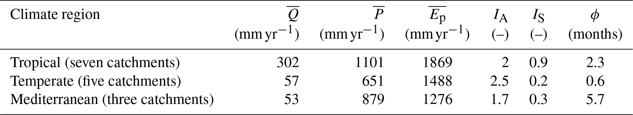
Table 1Average hydrological characteristics of the catchments in the three climate regions for the time period 1973–2010 with long-term mean annual discharge , long-term mean annual precipitation , long-term mean annual potential evaporation , aridity index , and the seasonality index of precipitation , where is the annual mean precipitation and the monthly mean precipitation in month m (Gao et al., 2014); ϕ is the time lag between long-term mean maximum monthly precipitation (P) and potential evaporation (Ep). Values for all individual catchments are provided in Table S2.
The objective of this study is to quantify and evaluate the effects of a climate-controlled representation of Sr on the water fluxes modeled by the Hydrology Tiled ECMWF Scheme for Surface Exchanges over Land (HTESSEL) land surface model. Specifically, we will test the hypothesis that implementing Sr,MM in HTESSEL can improve the modeled magnitude and timing of catchment discharge and evaporation fluxes. By applying the memory method for estimating ecosystem-scale Sr for use in LSMs, the first three limitations of using sparse root observations mentioned above can be overcome, but it should be acknowledged that, although the memory method in principle allows for adaptively updating Sr, in this work we use a fixed value in time. In this study, Sr,MM values representative for the 1973–2010 time period are estimated for 15 Australian catchments across different climate regions (Sect. 2.3 and Appendix A). The Sr,MM estimates are then used to constrain the Sr in HTESSEL (Sect. 2.5). Section 3 evaluates the effects on discharge and evaporation in HTESSEL by performing offline simulations with and without the improved representation of Sr. Finally, in Sects. 4 and 5 the potential for a wider application of climate-controlled root zone parameters is discussed.
2.1 Study area
Australia is characterized by large spatial differences in precipitation (Fig. 1), vegetation coverage and temperatures, varying from hot and dry deserts in the interior to tropical forests with a monsoon season in the north. We have selected 15 Australian river catchments with station observations of river discharge at the outlet of the catchment to estimate Sr by applying the memory method (Fig. 1; Table S1 in the Supplement) (Australian Government Bureau of Meteorology, 2019). The catchments are selected based on available discharge data (at least 30 years of station observations), size (at least one-third of the land surface model grid cell area of approximately 5500 km2 in order to spatially extrapolate catchment characteristics to grid cells) and differences in climate (spatial spread of the catchments across Australia for the analysis of different climate zones). The catchments are classified in three climate regions based on their hydrological characteristics (Table 1; Fig. 2; Table S2). The tropical catchments are characterized by pronounced seasonality of rainfall with a seasonality index of precipitation (IS) of 0.7 or higher, while temperate and Mediterranean catchments have year-round rainfall (IS<0.7). The Mediterranean catchments are characterized by a time lag ϕ between long-term mean maximum monthly potential evaporation Ep and precipitation P of 5 or 6 months, while in tropical and temperate catchments mean maximum monthly Ep and P occur within 3 months.
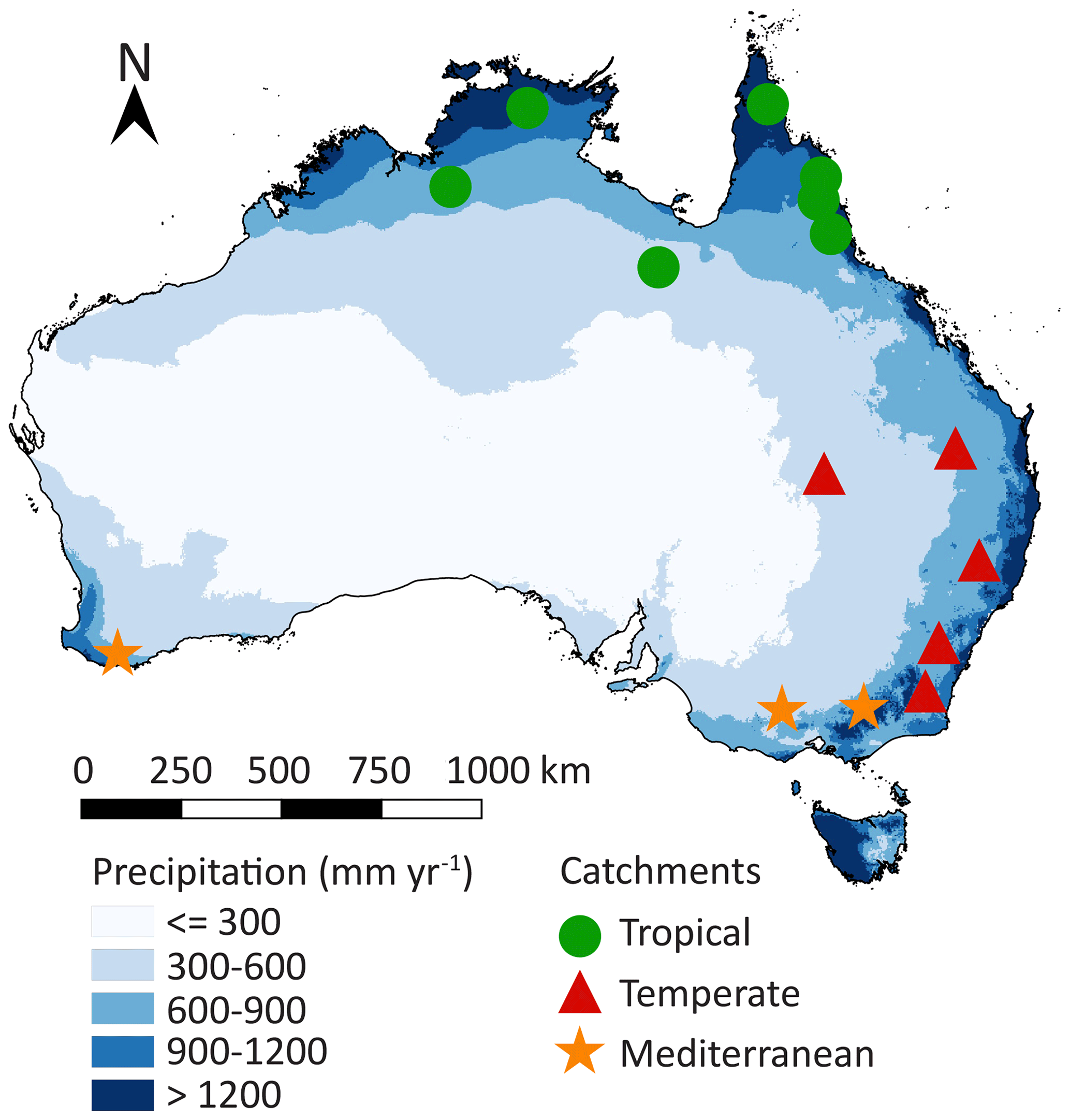
Figure 1Location of the 15 study catchments within Australia. The green, red and orange markers indicate the climate region, and the blue shades indicate long-term mean annual precipitation (Australian Government Bureau of Meteorology, 2019). A list of the catchments and their characteristics is provided in Table S1.
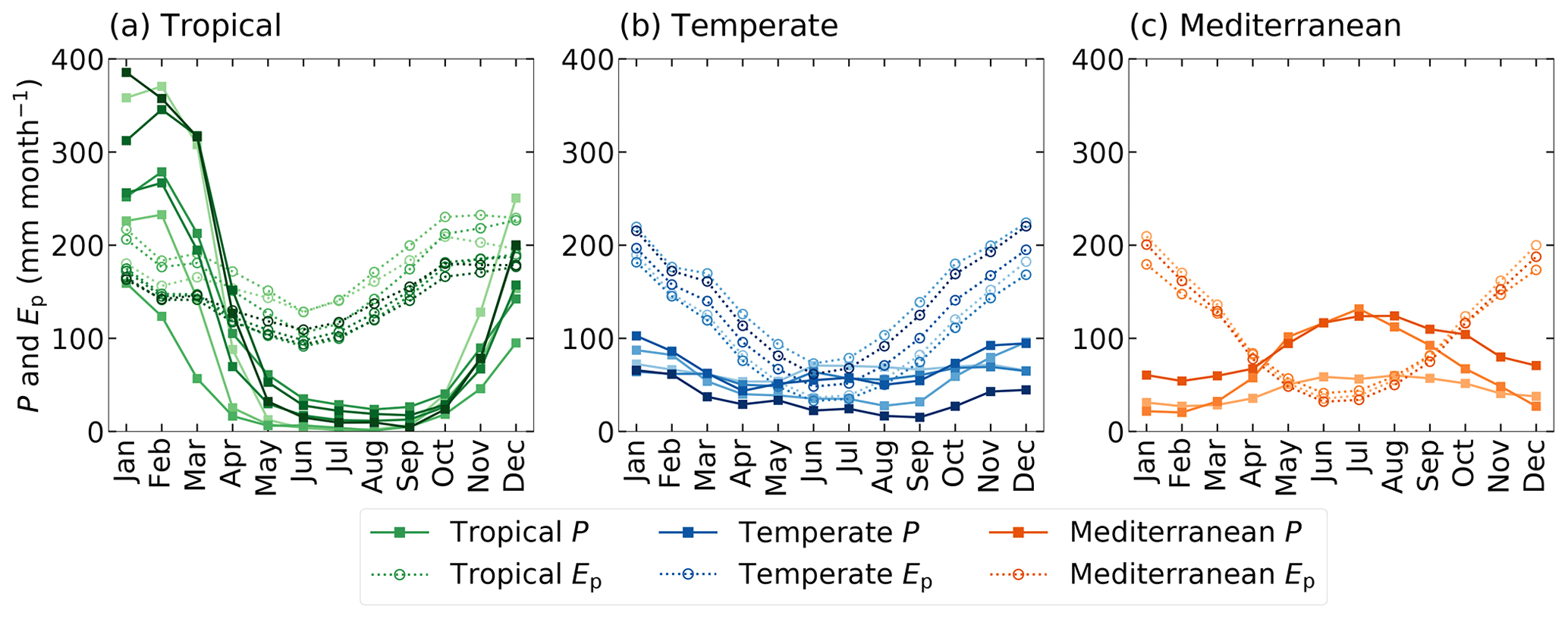
Figure 2Monthly seasonal climatology of precipitation (P) and potential evaporation (Ep) for the (a) tropical, (b) temperate and (c) Mediterranean catchments, with the solid lines representing P and the dashed lines Ep, for the time series 1973–2010. The different shades indicate the 15 individual study catchments.
2.2 Data
For this study we use daily discharge data from station observations in the catchments for the time period 1973–2010 (Australian Government Bureau of Meteorology, 2019). For the same time period we use daily precipitation and daily mean temperature data from the GSWP-3 dataset on a regular 0.5∘grid (Kim, 2017). Daily Ep is calculated by applying the Hargreaves and Samani formulation based on temperature and radiation (Hargreaves and Samani, 1982; Mines ParisTech solar radiation data, 2016). The FLUXCOM RS + METEO dataset is used as a reference dataset to benchmark modeled actual evaporation. FLUXCOM provides a gridded product of interpolated monthly evaporation as a fusion of FLUXNET eddy covariance towers, satellite observations and meteorological data (GSWP-3) for the time period 1975–2010 (Jung et al., 2019). This dataset has shown plausible estimates of mean annual and seasonal evaporation and is generally considered a suitable tool for global land model evaluations (Jung et al., 2019; Ma et al., 2020). However, we found considerable differences between the long-term annual mean evaporation and derived from the catchment water balance () based on observed Q and GSWP-3 P () (Fig. 3). Figure 3 clearly illustrates that the is consistently lower than , with an average difference of 150 mm yr−1, which is equivalent to about 20 % of the long-term water balances. is likely to be more reliable than because provides an integrated catchment-scale estimate as it is derived from observations of Q assuming that the catchments are large enough to neglect deep groundwater drainage to or from other catchments (Bouaziz et al., 2018; Condon et al., 2020). In addition, is based on point-scale estimates of FLUXNET stations that do not coincide with and are mostly located far from the study catchments (Pastorello et al., 2020). The discrepancy between the FLUXCOM and catchment water balance is addressed by scaling the monthly FLUXCOM evaporation:
with EFLUXCOM-WB as the monthly reference evaporation representative for the catchment scale, EFLUXCOM from Jung et al. (2019) in the catchment corresponding grid cells and the catchment-specific scaling factor.
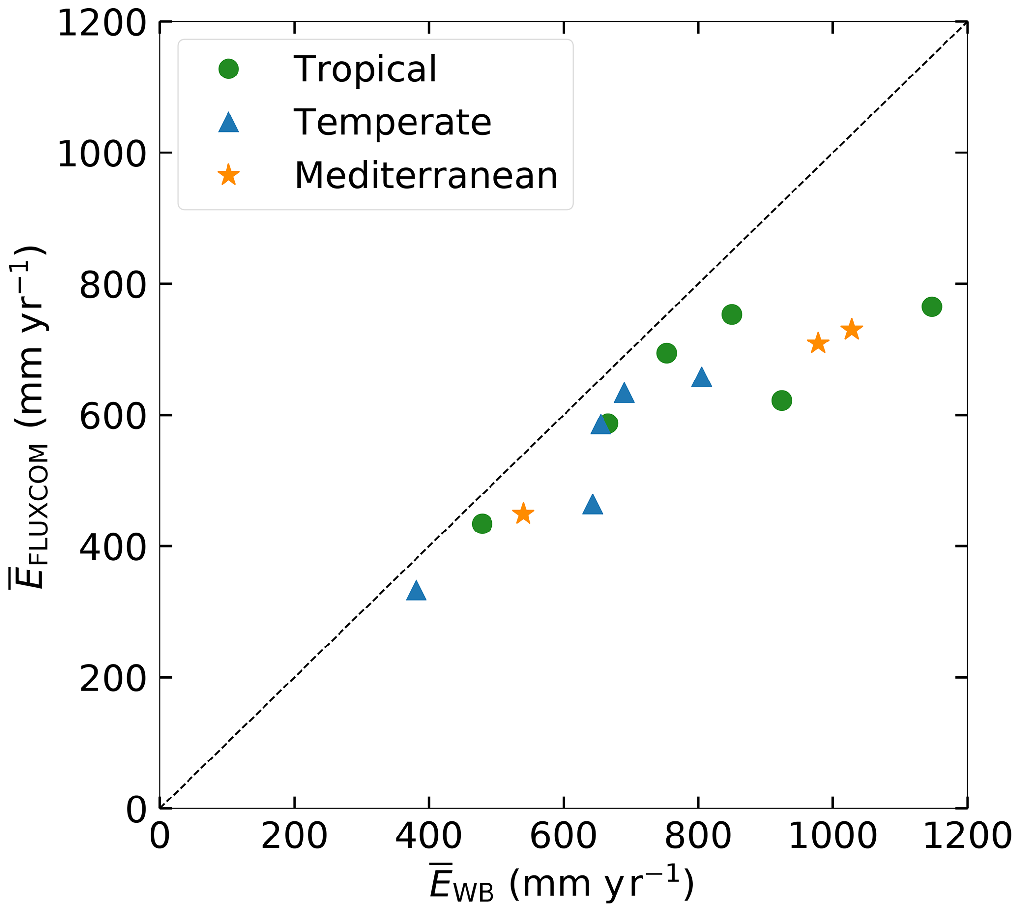
Figure 3Long-term mean annual evaporation () as estimated from long-term water balance data () compared to the FLUXCOM dataset () for the 1975–2010 period.
We use gridded data on vegetation type and coverage derived from the GLCC1.2 (ECMWF, 2016) and soil texture data from the FAO/UNESCO Digital Soil Map of the World (FAO, 2003). Characteristics of the different soil textures are based on the Van Genuchten soil parameters (Van Genuchten, 1980). These data are needed as input to the HTESSEL model and for the estimation of Sr.
2.3 Memory method for estimating root zone storage capacity
Sr,MM is estimated based on catchment hydrometeorological data according to the methodology described in the studies of De Boer-Euser et al. (2016), Nijzink et al. (2016) and Wang-Erlandsson et al. (2016). Sr,MM is based on an extreme value analysis of the annual maximum water storage deficits in the vegetation's root zone (Sd). Sd maximizes during dry periods, and therefore Sr represents an upper limit of root zone storage assuming that vegetation has sufficient access to water to overcome these dry periods. The cumulative water storage deficit Sd (mm) in the root zone is based on daily time series of effective precipitation Pe (mm d−1) and transpiration Et (mm d−1) for the time period 1973–2010 and is described by
with an integration from t0 that corresponds to the first day in the hydrological year 1973 to τ that corresponds to the daily time steps ending on the last day of the hydrological year 2010. Pe (mm d−1) is derived from the water balance of the interception storage Si:
with P representing the precipitation (mm d−1) and Ei the interception evaporation (mm d−1). Equation (3) can be solved by Eqs. (4)–(6). Herein, for the sum of fluxes between two time steps the following notation is used: , where F is either P, Ei, Pe or Ep (potential evaporation, mm d−1). The numerical solution was then thus obtained as follows using daily time steps.
Here, Si,max is the maximum interception storage (mm) that depends on the land cover and is estimated between 2–8 mm for a tropical forest (Herwitz, 1985) and between 0–3 mm for a temperate forest (Gerrits et al., 2010). However, De Boer-Euser et al. (2016) found that the sensitivity of Sr to the value of Si,max is small, and therefore a value of 2.5 mm is used here in all catchments for simplicity.
Daily Et (mm d−1) in Eq. (2) was calculated by
where c (−) is a coefficient that represents the ratio between transpiration and potential evaporation . (mm yr−1) is the long-term mean transpiration derived from the water balance () and (mm yr−1) the long-term mean potential evaporation. Et considered here includes both transpiration and soil evaporation, but as the latter is much smaller, we use the term transpiration for simplicity. The subtle interactions between atmospheric water demand and vegetation-available water supply can lead to interannual variability in c. The above-described approach that provided constant estimates of c is therefore extended by an iterative procedure to estimate annually varying values of the coefficient c as described in Appendix A.
Catchment Sr,MM (mm) is estimated based on the assumption that a catchment's ecosystem designs its rooting system while keeping memory of water stress events with certain return periods. Previous studies provide evidence that these return periods are likely to be longer for high vegetation (e.g., forest) than for low vegetation (e.g., grass). Based on the results of Gao et al. (2014), De Boer-Euser et al. (2016) and Wang-Erlandsson et al. (2016) drought return periods (RP) for high and low vegetation are set to 40 and 2 years, respectively. The Sr,MM corresponding to these drought return periods is calculated by applying the Gumbel extreme value distribution (Gumbel, 1935) to annual maximum storage deficits. Theoretically we could treat Sr separately for high and low vegetation in HTESSEL. However, this would require changing the root distributions (see Sect. 2.4), which we decided not to do as we did not want to change multiple parameters at the same time. Therefore, for the implementation of Sr,MM in HTESSEL, catchment Sr,MM is estimated as a weighted sum of the high and low vegetation Sr based on the coverage fraction of high (CH) and low (CL) vegetation in the corresponding grid cell of that specific catchment, described by
2.4 HTESSEL model description
In this study we use the Hydrology Tiled ECMWF Scheme for Surface Exchanges over Land (HTESSEL) land surface model (Balsamo et al., 2009). This section presents the model parameterization of vegetated areas in the HTESSEL control model version (hereinafter CTR) based on the IFS documentation of cycle CY43R1 and the model code itself (ECMWF, 2016). The core structure of this model is described by van den Hurk et al. (2000), and major changes in the hydrology parameterization were made by Balsamo et al. (2009) with the implementation of a global soil texture map instead of a single soil type and a runoff scheme accounting for sub-grid variability, which resulted in improvements in global water budget simulations (Balsamo et al., 2011).
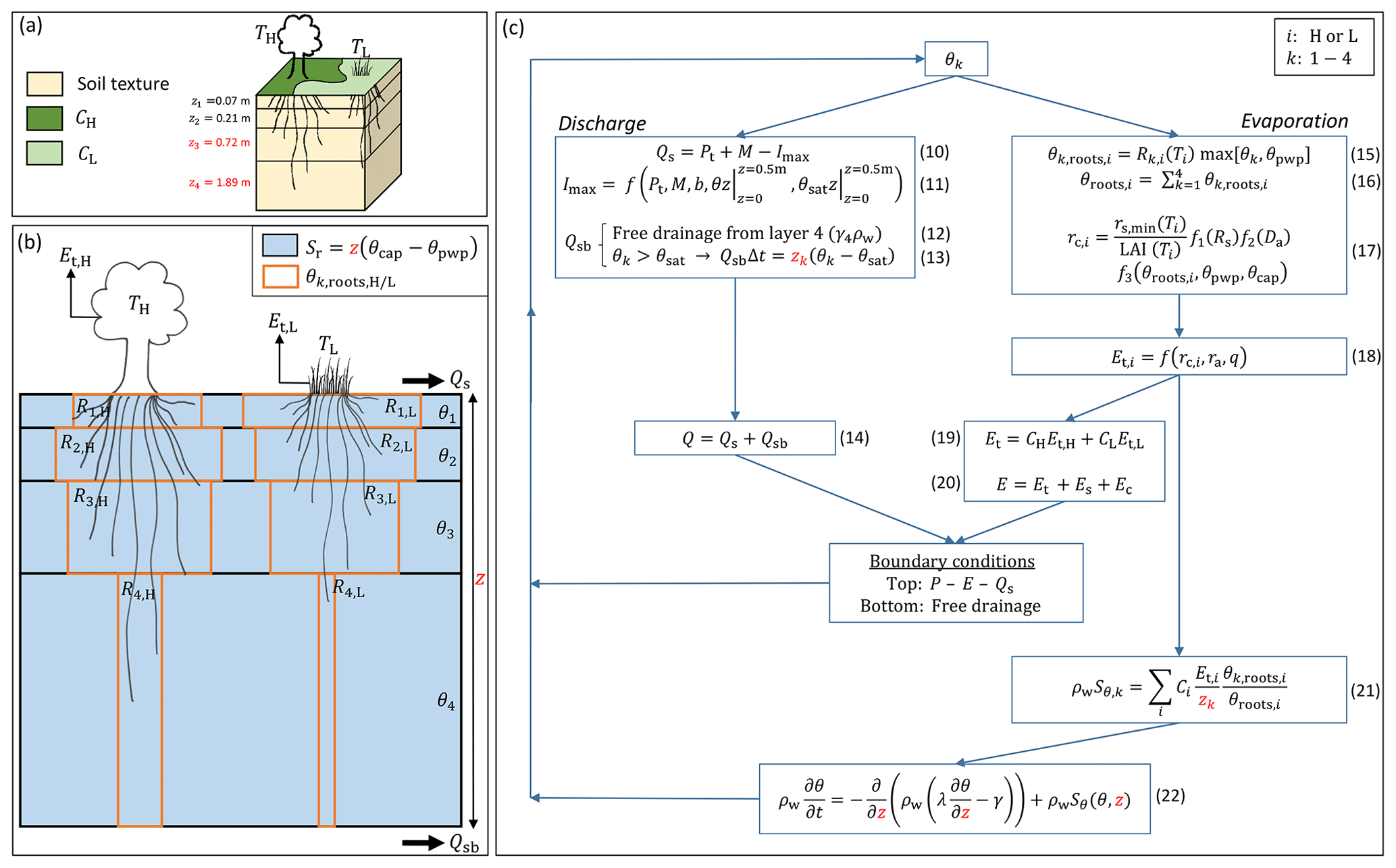
Figure 4Root zone parameterization in the HTESSEL CTR version with the directly changed parameters in the HTESSEL MD version highlighted in red. (a) 3D overview of a single grid cell. (b) Schematic image of the four-layer subsurface. (c) Scheme of equations for the calculation of soil moisture, discharge and evaporation. The symbols in this figure are as follows, with i representing high (H) and low (L) vegetation and k layers 1–4: C (−) vegetation coverage, T dominant vegetation type, z (m) layer depth, P (m s−1) precipitation, Pt (m s−1) precipitation through-fall, M (m s−1) snowmelt, Q (m s−1) total discharge, Qs (m s−1) surface runoff, Qsb (m s−1) subsurface runoff, Imax (m s−1) maximum infiltration rate, b (−) variable representing sub-grid orography, E (m s−1) total evaporation, Et (m s−1) transpiration, Es (m s−1) soil evaporation, Ec (m s−1) canopy evaporation, R (%) root distribution, θ (m3 m−3) unfrozen soil moisture, θpwp (m3 m−3) soil moisture at permanent wilting point, θcap (m3 m−3) soil moisture at field capacity, θsat (m3 m−3) soil moisture at saturation, Sr (m) the root zone storage capacity, θroots (m3 m−3) the root extraction efficiency, rc (s m−1) canopy resistance, ra (s m−1) atmospheric resistance, Rs (W m−2) downward shortwave radiation, Da (hPa) atmospheric water vapor deficit, q specific humidity (kg kg−1), rs,min (s m−1) minimum canopy resistance, LAI (−) leaf area index, Sθ () root extraction rate, γ (m s−1) hydraulic conductivity, λ (m2 s−1) hydraulic diffusivity and ρw (kg m−3) density of water.
Figure 4a represents a simplified 3D view of a single grid cell. The HTESSEL model describes eight different surface fractions within a grid cell (ECMWF, 2016), but we only considered the vegetation-covered fractions (high and low vegetation) because of the presence of roots. Considering exclusively vegetated areas, the grid cell surface is subdivided into high and low vegetation-covered area (CH and CL) with a dominant type of vegetation (TH and TL) based on the GLCC1.2 vegetation database. This database distinguishes 18 different vegetation types (e.g., evergreen broadleaf, tall grass, crops), each described with vegetation-specific parameters based on experiments and literature (e.g., minimum canopy resistance, root distribution). The subsurface has a single soil texture based on FAO (2003) and is subdivided into four model layers with a total depth z of 2.89 m that is kept uniformly constant in the global domain.
Figure 4b presents the connection of the subsurface with the surface through roots and transpiration fluxes (Et) in more detail. Sr is not explicitly described in the model parameterization, and therefore it is formulated based on our own understanding of its relation to the HTESSEL vegetation and root zone parameterizations (Eq. 9). Vegetation has roots in all four model soil layers (except for the vegetation types desert and tundra that can only access the upper layer and the upper three layers, respectively; ECMWF, 2016). There is a variable root distribution across the layers that is different for each vegetation type. The vegetation-specific root distribution (Rk) describes the root fraction with respect to the total amount of roots in each model soil layer. At a single time step, the capability of roots to extract soil moisture (θk,roots, represented by the brown boxes in 4b) is a function of Rk and the layer of unfrozen soil moisture content (θk). Thus, the more roots we have in a soil layer, the more moisture can be extracted at each time step. In the long term, however, the vegetation is able to extract all the plant-available soil moisture in the layers where roots are present. Therefore, Sr,CTR, represented in blue in Fig. 4b, is described by
with z representing the hydrologically active depth, which corresponds to the combined depth of all soil layers with roots (z=2.89 m is a default value in HTESSEL for all vegetation types except for desert and tundra), and θcap−θpwp the plant-available moisture, which is constant over the four soil layers. The plant-available moisture is bounded by the soil-texture-specific moisture contents at field capacity (θcap), above which soil moisture drains by gravity, and at the wilting point (θpwp), below which soil moisture is not accessible to roots. It should be noted that we aimed for a physical definition of Sr,CTR but that the effective water used by vegetation may be different. We come back to this point more elaborately in the Discussion section (Sect. 4.3).
Figure 4c presents the equation scheme of HTESSEL for calculating soil moisture as well as discharge and evaporation fluxes, with i representing high (H) or low vegetation cover (L) and k the four soil layers. The relative soil moisture content θ controls the calculations of discharge and evaporation fluxes. The surface runoff (Qs) is defined by the precipitation through-fall (Pt), snowmelt (M) and maximum infiltration rate (Imax) (Eq. 10). Imax is a function of Pt, M, a spatially variable parameter (b) that is defined by the standard deviation in sub-grid orography, and the vertically integrated (top 0.5 m) soil moisture (θ) and saturation soil moisture (θsat) (Eq. 11) (Dümenil and Todini, 1992; van den Hurk and Viterbo, 2003). The subsurface runoff (Qsb) consists of two components: free drainage from layer 4, which is a function of hydraulic conductivity in this layer (γ4) and water density (ρw) (Eq. 12), and the excess absolute soil moisture when θk>θsat (Eq. 13). Total discharge (Q) is the sum of Qs and Qsb (Eq. 14), and as typical in-stream travel times through the catchments are about 1 d at most, we did not consider routing to be important at the monthly timescale for which we analyze the results. The average root extraction efficiency in all layers (θroots) is described by Eqs. (15) and (16) as the weighted sum of the vegetation-specific Rk and θk. The canopy resistance (rc) (Eq. 17) describes the resistance of vegetation to transpiration and is a function of vegetation-specific values for minimum canopy resistance (rs,min) and LAI, a function of shortwave radiation (f1(Rs)), a function of atmospheric water vapor deficit (f2(Da)) and a function of the root extraction efficiency (). The canopy resistance defines Et,i together with specific humidity (q) and an atmospheric resistance term (ra) (Eq. 18). Total Et is a weighted sum of the separate transpiration products based on the sub-grid coverage CL and CH (Eq. 19), and total evaporation (E) is a sum of transpiration (Et), soil evaporation (Es) and canopy evaporation (Ec) fluxes (Eq. 20). The detailed formulations of the latter two fluxes are not relevant in this study and are therefore not included in this model description. Et,i is attributed to the different soil layers in the calculation of the root extraction (Sθ) based on the layer depth (zk) and θk,roots (Eq. 21). The change in soil moisture over time () is calculated by applying the Darcy–Richards equation with γ and λ representing hydraulic conductivity and diffusivity (Eq. 22). This equation is solved with a top soil boundary condition of and a bottom soil boundary condition of free drainage.
2.5 Implementation of memory method root zone storage capacity estimates in HTESSEL
Here we develop an approach to implement the climate-controlled Sr,MM (results in Sect. 3.1) in HTESSEL, while maintaining the modeling framework of the CTR model described in Sect. 2.4. We found that Sr,CTR is exclusively defined by the soil type and the hydrologically active model soil depth (z) (Eq. 9). In our modified version of HTESSEL, hereafter referred to as the Moisture Depth (MD) model, the soil depth for moisture calculations is changed to satisfy the following equation:
with zMD as the total soil depth in the MD model modified to satisfy Sr,MD=Sr,MM. This depth change is achieved by changing model layer 4, except in the case that this would cause the model depth of layer 4 to approach zero (z4≈0). In this case a minimum threshold (0.2 m) is set for z4, and the depth of layer 3 is further changed to obtain Sr,MD=Sr,MM as required in Eq. (23). This is necessary because z4≈0 in the moisture calculation would cause inconsistencies in the thermal diffusion calculations as the layer soil temperature is a function of the layer soil moisture. The layer depths for thermal diffusion calculations are not modified in the MD model, and we found that the soil layer temperatures are insensitive to depth changes in MD. The directly changed parameters in MD are highlighted in red in Fig. 4. Also, the root distribution is not modified in MD because we aimed for a physical representation of Sr (Eq. 23) and we did not want to change multiple model parameters at the same time. Furthermore, we would like to reiterate that the soil depth in the model should be interpreted neither as actual soil depth nor rooting depth, but merely as a way to represent the plant-accessible water volume.
2.6 Model simulations
Simulations are performed in a stand-alone version of HTESSEL (Balsamo et al., 2009) as it was implemented in the framework of version 3 of the EC-EARTH Earth system model (http://www.ec-earth.org, last access: August 2020) for both the CTR (Sect. 2.4) and MD (Sect. 2.5) model versions. The model is forced with 3-hourly GSWP-3 atmospheric boundary conditions (Kim, 2017) for the historical time series 1970–2010, with the first 5 years used for spin-up. The spatial resolution of the HTESSEL model is a reduced Gaussian grid (N128), with the grid cells over Australia being approximately 5500 km2.
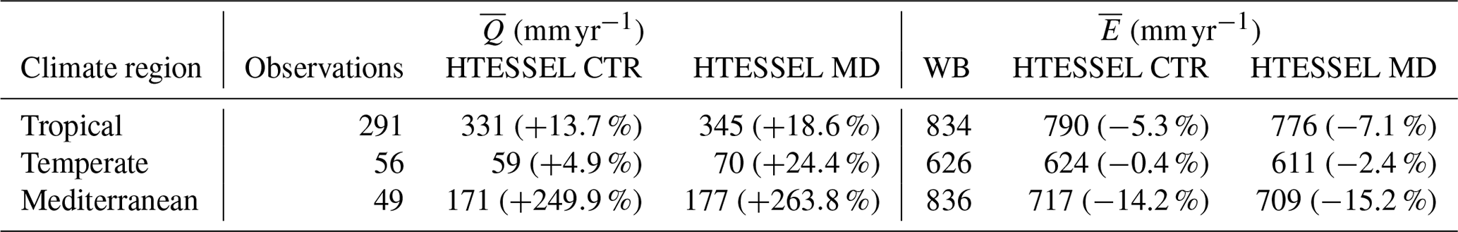
Table 2Long-term annual mean modeled discharge () and evaporation () in the HTESSEL CTR and MD versions for the tropical, temperate and Mediterranean climate regions (catchment averages) as well as reference (station observations) and (, Sect. 2.2). The p biases of the modeled climate region average and are presented between brackets. Similar values for the individual catchments are shown in Tables S3 and S4.
2.7 Model evaluation
Most study catchments are smaller than single HTESSEL grid cells (Table S1). For catchments completely falling within a single HTESSEL grid cell, this cell is selected for analysis. In the case that a catchment falls within more than one grid cell, the average of the model output in the separate grid cells is used for analysis. The model performances of CTR and MD are compared based on modeled monthly discharge and evaporation fluxes for 1975–2010: long-term annual means, monthly seasonal climatology and interannual anomalies of monthly fluxes (monthly fluxes minus monthly climatology) are evaluated. Modeled Q is compared to station observations and modeled E to the FLUXCOM-WB evaporation (Sect. 2.2 and Eq. 1). For long-term annual means, the percent bias between the reference and modeled fluxes is calculated (evaporation ). For the monthly seasonal climatology and interannual anomalies, the model performance is quantified by using the Pearson correlation coefficient (r) and a variability performance metric () that depends on the ratio of modeled and reference standard deviation (). These performance metrics are calculated for the individual catchments and then averaged to evaluate model performance over tropical, temperate and Mediterranean climate regions.
To test the significance of the improvement in model performance of MD compared to CTR, a Monte Carlo bootstrap method (1000 repetitions) is employed. The 1000 samples are taken by randomly resampling with replacement among CTR and MD values at each time step. The null hypothesis of getting as high or higher performance parameters simply by chance is tested at the 5 % and 10 % significance levels for the individual catchments as well as for the performance averages over the tropical, temperate and Mediterranean climate regions. P values of the model improvements are provided in Tables S5 and S6.
3.1 Root zone storage capacity estimates
Figure 5 shows that there is no relation between Sr,MM and Sr,CTR. The range of Sr,MM (125–722 mm) in the study catchments is much larger than the range of Sr,CTR (491–725 mm), indicating that HTESSEL may not adequately represent the spatial heterogeneity of Sr (Table S2). The range of Sr,MM in the catchments is consistent with Wang-Erlandsson et al. (2016), who found similar ranges of Sr (approximately 100–600 mm) over Australia by using gridded products of Sr based on rooting depths from observations and optimized inverse modeling, and they also found similar ranges of global Sr,MM estimated based on satellite evaporation products. Sr,MM estimates are on average smaller in the five temperate (194 mm) catchments than in the three Mediterranean (321 mm) and the seven tropical (437 mm) catchments. In the tropical and Mediterranean regions vegetation needs to bridge extensive dry seasons as rainfall seasonality is high (Fig. 2, Table 1), resulting in larger Sr,MM than in temperate regions with year-round precipitation. In the Mediterranean, the average time lag between P and Ep of 5.7 months results in large root zone storage deficits in the hot and dry summers and therefore larger Sr,MM than in the temperate catchments.
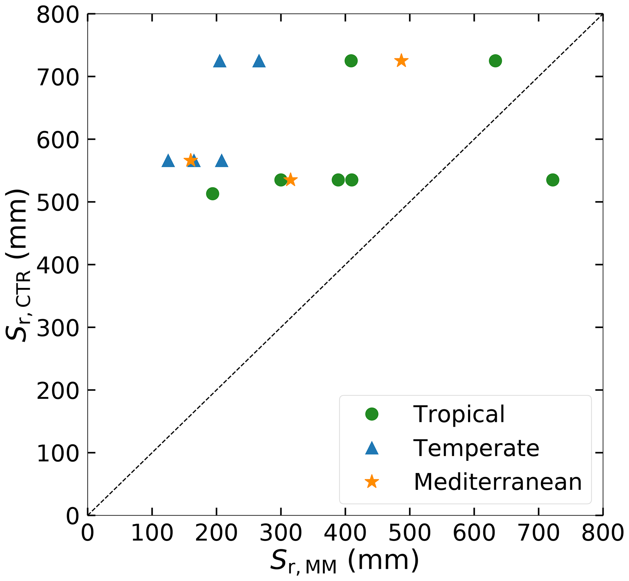
Figure 5Catchment Sr as estimated from the memory method (Sr,MM) compared to the HTESSEL CTR parameterization (Sr,CTR) in the catchment corresponding grid cells.
3.2 Long-term mean annual climatology
The HTESSEL CTR version overestimates observed in 9 out of 15 catchments with on average 40 mm yr−1 (tropical), 3 mm yr−1 (temperate) and 122 mm yr−1 (Mediterranean) (Tables 2, S3 and S4). This overestimation of observed Q goes together with an average underestimation of by CTR. As Sr,MM is generally smaller than Sr,CTR (Fig. 5), the MD version results in reduced and increased compared to CTR, but the changes are quite small (Table 2). The MD increase in modeled compared to CTR results on average in larger p biases in tropical (+16.9 % vs. +13.7 %), temperate (+24.4 % vs. +4.9 %) and Mediterranean (+263.8 % vs. +249.9 %) catchments, but the results are largely variable among the individual catchments (Table S4).
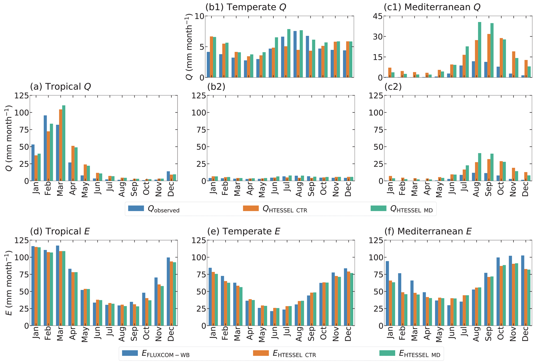
Figure 6Monthly seasonal climatology of observed discharge (Q) (a–c) and FLUXCOM-WB evaporation (EFLUXCOM-WB) (d–f) as well as modeled values in the HTESSEL CTR and MD versions, averaged for the tropical (a, d), temperate (b, e) and Mediterranean (c, f) catchments for the time series 1975–2010. Labels (b1) and (c1) represent the same data as in (b2) and (c2), but with a different y axis. Similar illustrations for the individual catchments are shown in Figs. S1 (Q) and S2 (E).
3.3 Monthly seasonal climatology
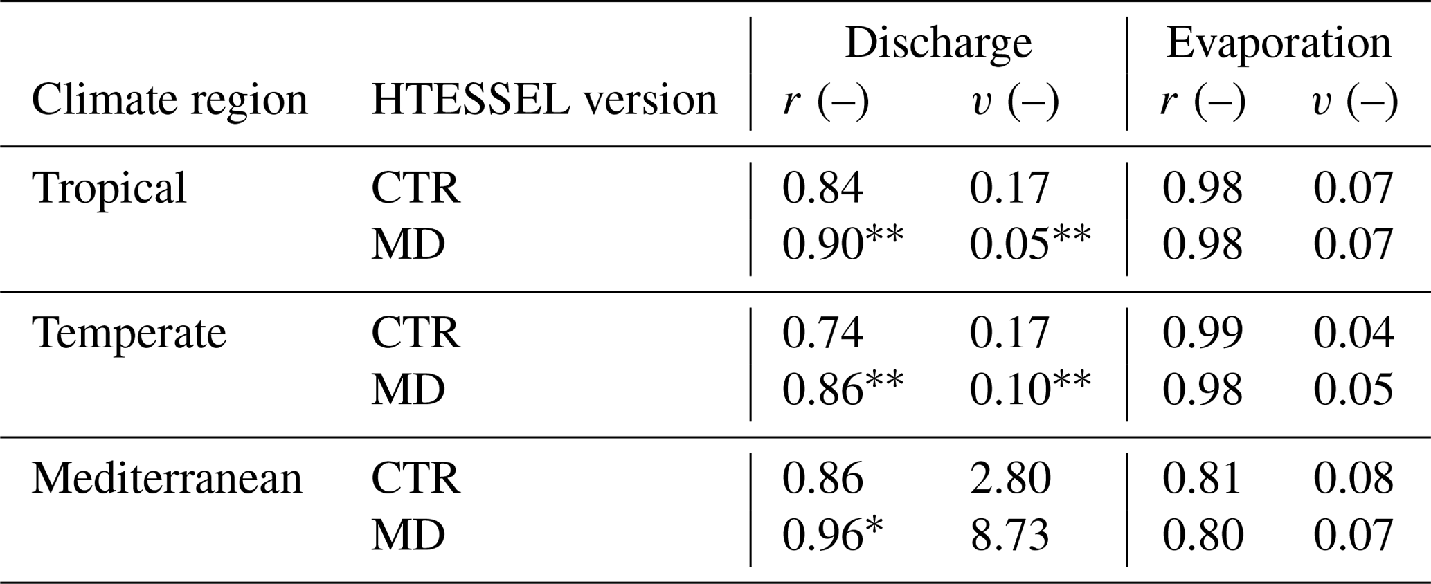
Although does not considerably change in MD compared to CTR (Sect. 3.2), MD reproduces the seasonal variations in Q considerably better than CTR (Fig. 6a–c and Table 3). In the tropical and Mediterranean catchments, MD increases Q in the wet months, while it decreases Q in the dry months compared to CTR and hence improves the seasonal timing of observed Q (Fig. 6a, c and Table 3). In the temperate catchments, MD increases Q in the wet months (July–September) compared to CTR in accordance with observations, although in the other months the changes in MD compared to CTR are mixed (Fig. 6b). In terms of the correlation between modeled and observed monthly seasonal climatology, Q improved in MD compared to CTR in 12 out of 15 catchments, with 7 catchments passing the 5 % significance level for improvement (Table S5). For the climate region averages, the correlation significantly improved in MD from 0.84 to 0.90 (tropical), from 0.74 to 0.86 (temperate) and from 0.86 to 0.96 (Mediterranean) compared to CTR (Table 3). On average, MD resulted in larger variations in monthly Q than CTR (Fig. 6a–c). The variability term improved from 0.17 to 0.06 (tropical) and from 0.17 to 0.10 (temperate) in MD compared to CTR, but in the Mediterranean catchments the models strongly overestimate the observed variations in Q (Fig. 6c), with the variability term increasing from 2.80 in CTR to 8.73 in MD (Tables 3 and S5).
Table 3Model performance parameters of monthly seasonal discharge (Q) and evaporation (E) climatologies (1975–2010), with r representing Pearson correlation and variability (where ), in tropical, temperate and Mediterranean climate regions for the HTESSEL CTR and MD versions (catchment averages). Modeled Q is compared to station observations and modeled E to FLUXCOM-WB (Eq. 1). For r, a value of 1 represents a perfect model; for v a value of 0 represents a perfect model. The significance test of the MD improvements compared to CTR is represented by (passing the 5 % level) and * (passing the 10 % level). Values of r and α for the individual catchments and p values of improvement are shown in Tables S5 (Q) and S6 (E).
In contrast to the improvement in the monthly seasonal climatology of Q in MD, the monthly seasonal cycle of E appears not to be significantly affected, as shown in Fig. 6d–f and Table 3.
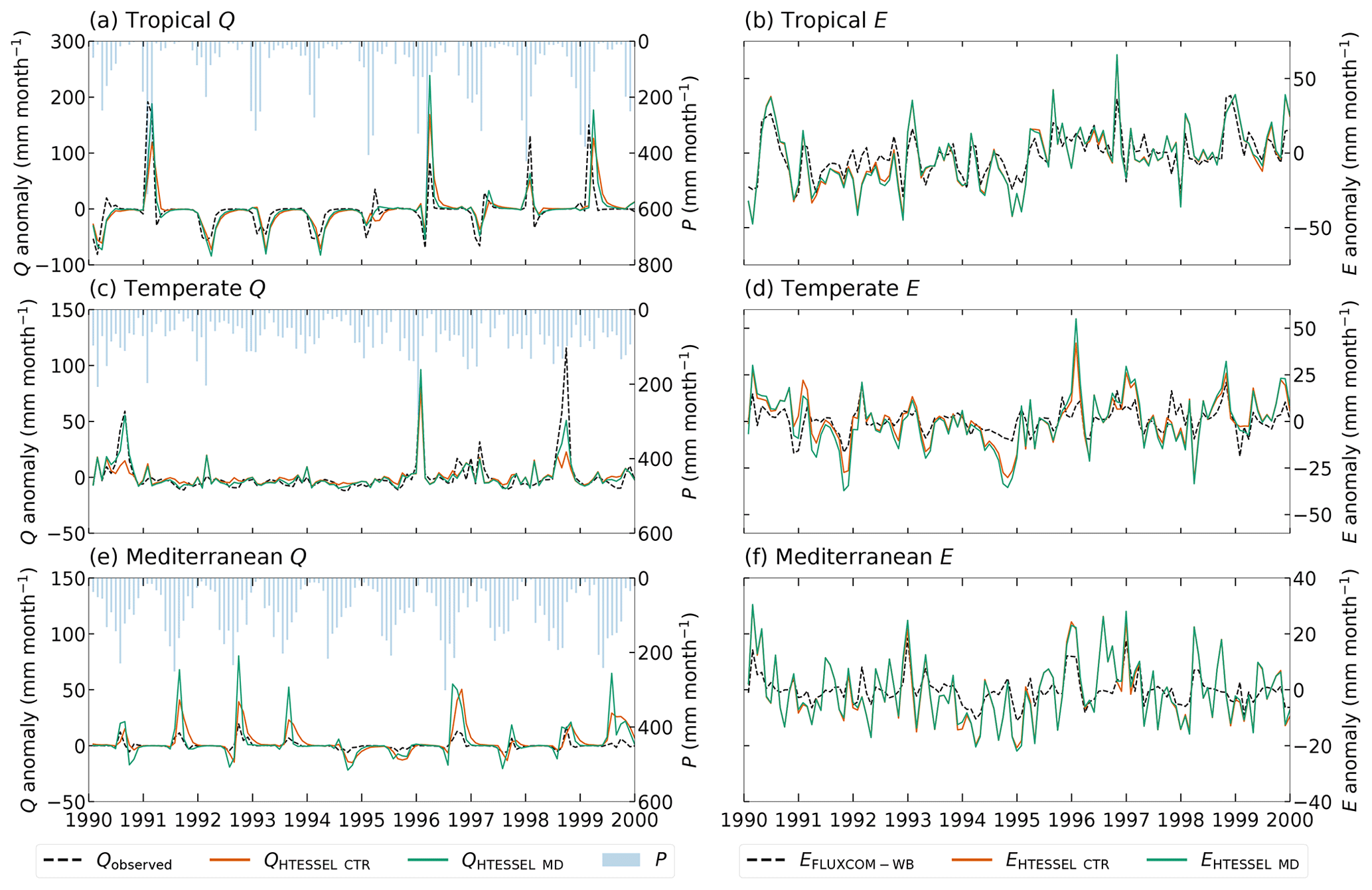
Figure 7Interannual monthly anomalies of observed discharge (Q) (a, c, e) and FLUXCOM-WB evaporation (E) (b, d, f) fluxes as well as modeled values in the HTESSEL CTR and MD versions in an individual representative tropical (catchment Mi) (a, b), temperate (catchment Na) (c, d) and Mediterranean (catchment K) (e, f) catchment based on the time series for 1975–2010. Similar illustrations for the individual catchments are shown in Figs. S1 (Q) and S2 (E).
3.4 Interannual monthly anomalies
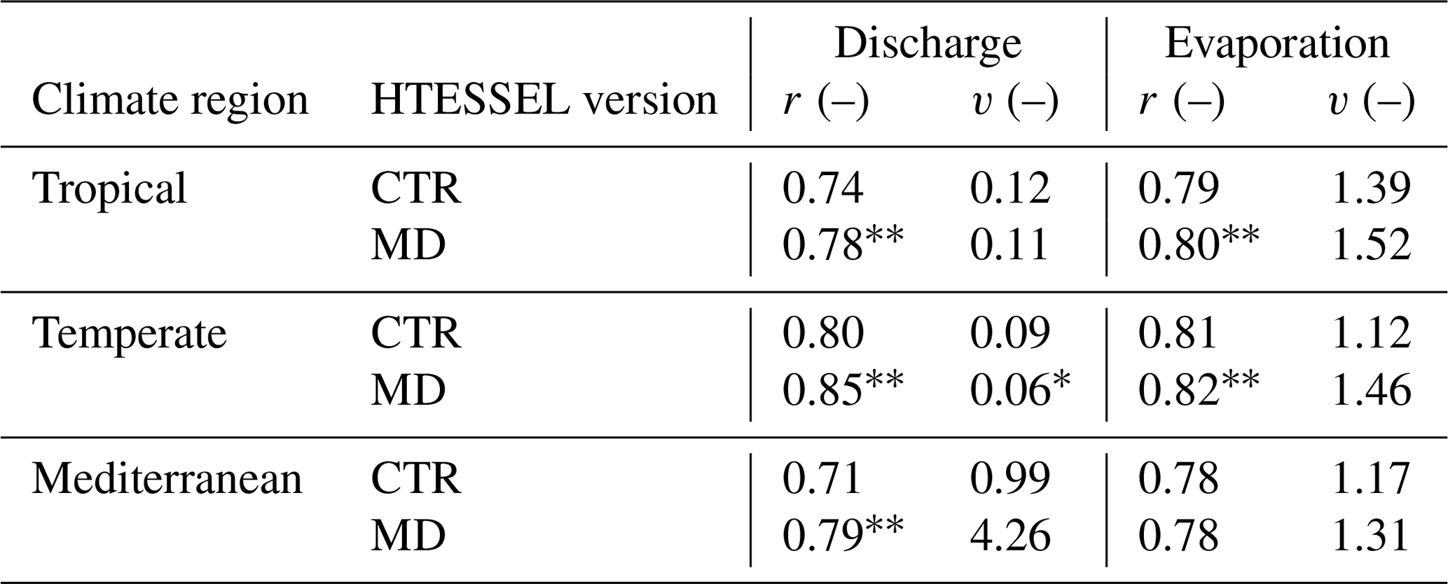
Figure 7a and c show that MD is better in capturing the variations in interannual Q anomalies than CTR in the presented tropical and temperate catchments, while in the Mediterranean catchment both models strongly overestimate the interannual Q anomalies compared to observations (Fig. 7e). In 14 out of 15 catchments, the variability in the interannual Q anomalies increases in MD compared to CTR (Fig. S1 in the Supplement and Table S5). This results in an average improvement in the interannual anomaly variability (v) from 0.12 to 0.11 (tropical) and from 0.09 to 0.06 (temperate) in MD compared to CTR (Table 4). However, in the Mediterranean catchments, the increased variability in the Q anomalies leads to a strong overestimation of Q anomalies with respect to observations (Figs. 7e and S1m–o), with v increasing from 0.99 in CTR to 4.26 in MD. Figure 7a, c and e also show that the timing of the Q anomalies improves in MD compared to CTR; in particular, the improved timing of the falling limbs is clearly visible in Fig. 7a and e. The interannual Q anomaly correlation (corresponding to the timing) improves in 14 out of 15 catchments, with 9 catchments passing the 5 % significance level for improvement (Table S5). On average, the correlation (r) increases from 0.74 to 0.78 (tropical), from 0.80 to 0.85 (temperate) and from 0.71 to 0.79 (Mediterranean) in MD compared to CTR. In contrast to the improvement in the interannual Q anomalies in MD, the interannual E anomalies do not considerably change compared to CTR (Fig. 7b, d and f; Tables 4 and S6).
4.1 Synthesis of results
Sr,MM is lower than Sr,CTR in 14 out of 15 catchments (Fig. 5). This is seemingly in contrast to literature suggesting that the root depth in land surface models is too low and that the absence of deep roots is a cause for uncertainties in simulated evaporation (Kleidon and Heimann, 1998; Pan et al., 2020; Sakschewski et al., 2020). However, Sr represents a conceptual water volume that is accessible to roots without defining where this volume is in reality. Therefore, it is not necessarily proportional to root depth as a small Sr does not preclude the presence of deep roots, as illustrated in Fig. 4 in Singh et al. (2020).
The modeling results show that the difference in long-term mean and fluxes between CTR and MD are small (Table 2), whereas the differences between monthly (climatological and interannual) variations are clearly visible (Figs. 6 and 7). This corresponds to other studies on catchment hydrology that suggest that the root zone storage mainly affects the fast hydrological response of a catchment (Oudin et al., 2004; Euser et al., 2015; Nijzink et al., 2016; De Boer-Euser et al., 2016). Furthermore, previous studies found larger improvements in modeled discharge using Sr,MM in humid regions with large rainfall seasonality (De Boer-Euser et al., 2016; Wang-Erlandsson et al., 2016). This is not found in our study, as we obtain slightly smaller improvements in the discharge correlation for the tropical catchments than for the temperate and Mediterranean ones. This is at least partly related to the smaller difference between Sr,MM and Sr,CTR in the tropical catchments than in temperate and Mediterranean ones (Fig. 5). The Mediterranean catchments have large climatological biases and overly large discharge variability in the seasonal cycle and interannual anomalies in CTR, and MD further degrades the performance with respect to bias and variability (Tables 2–4). On the other hand, the correlation of seasonal climatology and interannual anomalies consistently improves in all climate regions with the implementation of Sr,MM. Therefore, it is suggested that aspects of the hydrology parameterization other than Sr (e.g., the lack of a groundwater layer) could be primarily leading to the large climatological biases and overly large discharge variability in the seasonal cycle and interannual anomalies in the Mediterranean. On the other hand, uncertainties in the GSWP-3 forcing could also partly cause the large biases in the Mediterranean. In this climate region, it is found that GSWP-3 (0.5∘grid) is considerably larger than from the SILO dataset, which provides P on a 0.05∘grid directly derived from ground-based observational data (Jeffrey et al., 2001).
Table 4Model performance parameters of interannual monthly discharge (Q) and evaporation (E) anomalies (1975–2010), with r representing Pearson correlation and variability (where ), in tropical, temperate and Mediterranean climate regions for the HTESSEL CTR and MD versions (catchment averages). Modeled Q is compared to station observations and modeled E to FLUXCOM-WB (Eq. 1). For r, a value of 1 represents a perfect model; for v a value of 0 represents a perfect model. The significance test of the MD improvements compared to CTR is represented by (passing the 5 % level) and * (passing the 10 % level). Values of r and α for the individual catchments and p values of improvement are shown in Tables S5 (Q) and S6 (E).
Although we found significant differences in modeled Q between CTR and MD, the discrepancy in E was very limited in all climate regions (Tables 3, 4 and S6; Fig. S2). As stated before, the reliability of the FLUXCOM E is questionable in our study catchments (Fig. 3). Although the model performance with respect to E fluxes is uncertain, the lack of evaporation sensitivity to Sr was unexpected and requires more in-depth evaluation of the results in view of the HTESSEL model parameterization.
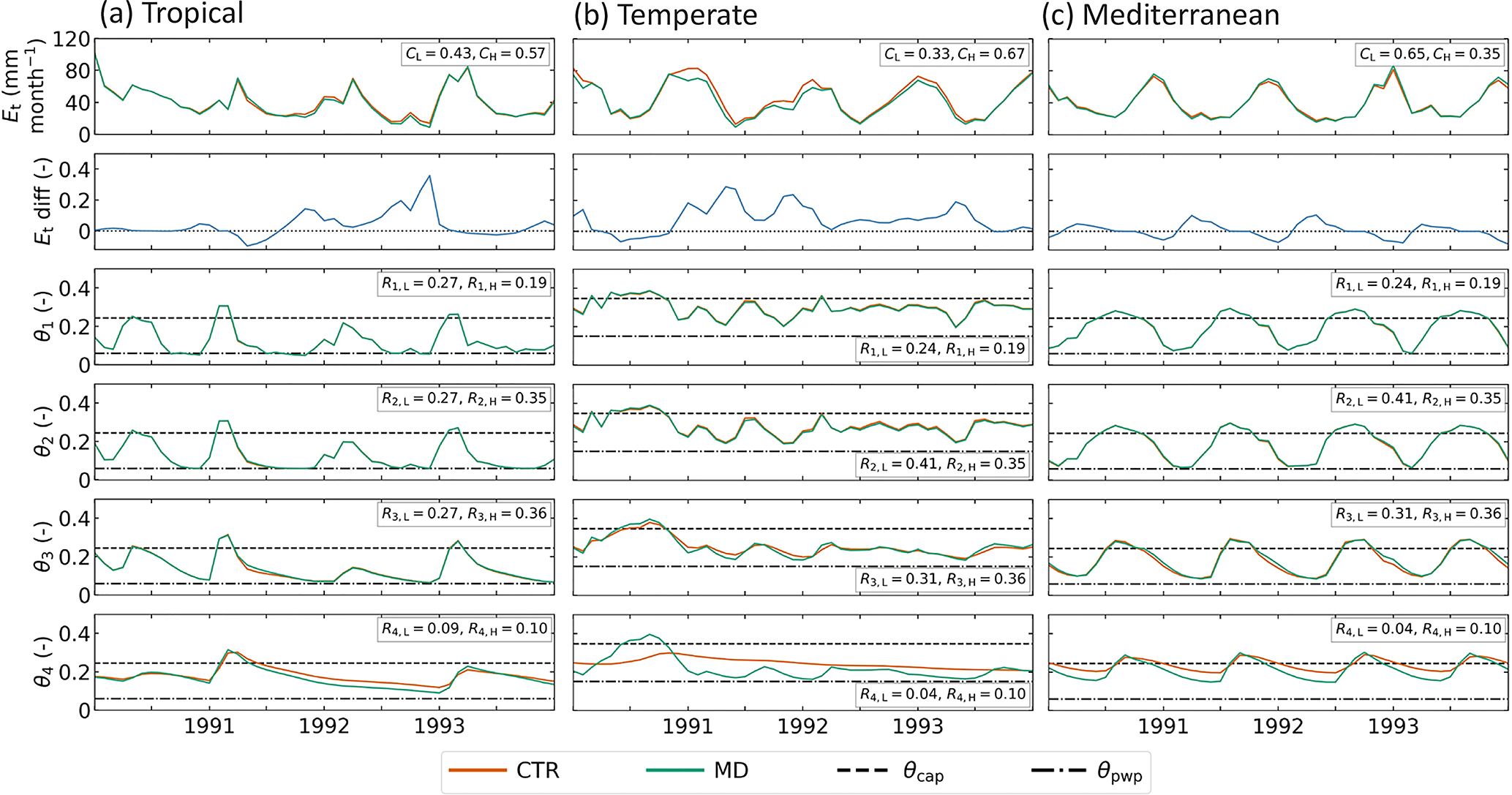
Figure 8Modeled transpiration and soil moisture content in the HTESSEL CTR and MD versions in an individual representative tropical (catchment Mi) (a), temperate (catchment Na) (b) and Mediterranean (catchment K) (c) catchment. From top to bottom: transpiration, relative difference between CTR and MD transpiration (), soil moisture layer 1, soil moisture layer 2, soil moisture layer 3, soil moisture layer 4. Additionally, the vegetation coverage (CL and CH) and the relative rooting distribution (Rk) for the dominant high and low vegetation types are presented.
In order to further explain the evaporation (in)sensitivity, we analyzed the modeled soil moisture and specifically looked at a wet period (mid-1990) and a dry period (beginning of 1991) in a temperate catchment, as shown in Fig. 8b. During the wet period, soil moisture in the upper three layers is above or close to θcap for both MD and CTR, while in the fourth layer MD has larger soil moisture than CTR. In this case evaporation is not moisture-limited and controlled by the top three layers because of the larger root distribution in these layers (Eqs. 14 and 15). Therefore, the modeled transpiration is not sensitive to the increase in layer 4 soil moisture in MD compared to CTR. During the transition from wet to dry periods, the upper three layers dry out first as there is a reduction in precipitation input. As these layers are relatively dry, evaporation is controlled by the fourth layer in which θ is reduced to values close to θpwp in MD, while it remains relatively wet in CTR. It is this difference in θ4 that causes the sensitivity of transpiration in MD during the wet-to-dry transition. However, most of the time the modeled soil moisture is in the wet and insensitive regime, and therefore the overall effect of MD on modeled evaporation tends to be small in the catchments considered in this study. To further analyze the evaporation sensitivity to Sr changes, it would be useful to evaluate to what extent it is model-dependent and compare HTESSEL behavior with other LSMs in a multi-model context (e.g., van den Hurk et al., 2016; Ardilouze et al., 2017). On the other hand, we also expect the evaporation sensitivity to Sr to be related to the methodology applied, which will be further discussed in Sect. 4.3.
4.2 Methodological uncertainty
Although the catchments were selected carefully, their location and sizes do not completely match the HTESSEL grid cells. Thus, assuming a one-to-one relation between precipitation, evaporation, river discharge and root zone storage capacities at the catchment and the grid cell is a potential source of error. However, this configures as random error and is therefore likely to cancel out in multiple catchment settings as is done in this study. Another source of uncertainty is the parameterization of the memory method for estimating catchment Sr. This method requires estimations of maximum interception storage, seasonal and interannual transpiration signals, and return periods, which lead to differences in Sr,MM when other values are chosen. A sensitivity analysis of Sr,MM with a high Sr,MM (Si,max=1.5 mm, RPlow=3 years, RPhigh=60 years, f=0.15; see Appendix A) and a low Sr,MM (Si,max=3.5 mm, RPlow=1.5 years, RPhigh=20 years, f=0.35) on average deviated 45 mm from the average Sr,MM estimates used in this study (Si,max=2.5 mm, RPlow=2 years, RPhigh=40 years, f=0.25). This deviation is small considering the average Sr,MM of 319 mm. In addition, irrigation, as a possible external water source in catchments with crops (Table S1), and deep groundwater, as a water source for deep-rooting vegetation, are not accounted for in the approach. However, we think that the estimation of transpiration is the main uncertainty in the approach. The assumption that the seasonal variations in Et and Ep are in phase may not hold in Mediterranean regions where Ep and P, and thereby the water available for transpiration, tend to be out of phase. Applying the seasonal pattern of transpiration modeled by CTR to the memory method in Mediterranean catchments results in smaller Sr,MM estimates in these catchments (average: 292 mm) than with the initial approach whereby the seasonality of Et was based on Ep (average: 321 mm). The relatively low deviation for both the parameter uncertainty and the uncertainty in the timing of Et leads us to conclude that these assumptions have a small impact on the general finding that Sr,MM is lower than Sr,CTR and that HTESSEL does not represent the spatial heterogeneity of Sr.
Station observations of river discharge are used in both the Sr,MM estimation and the model evaluation. However, because the memory method is only based on observations of long-term annual mean discharge () and the model evaluation is mainly based on the monthly seasonal and interannual variations in Q, we consider model evaluation based on these data appropriate.
4.3 Root zone storage capacity implementation
The HTESSEL CTR version does not explicitly formulate Sr, and therefore we formulate Sr,CTR based on the root zone parameterization as presented in Sect. 2.4 in order to modify the model parameters in a way to make the model consistent with the Sr,MM estimates. This formulation represents the theoretical Sr,CTR, but it may not fully correspond to the soil moisture in the four layers that is actually used by the modeled vegetation. The effective Sr (Sr,CTR,eff) can be derived a posteriori from the modeled soil moisture storage deficits and an extreme value analyses as done in the memory method (Sect. 2.3). Sr,CTR,eff is smaller than Sr,CTR based on depths (Fig. S3c), which is likely related to the relatively small root percentage in layer 4 compared to the other layers for most vegetation types (ECMWF, 2016). On the other hand, the Sr,MM we implemented in MD by changing soil depths is close the Sr,MD,eff based on modeled soil moisture deficits in MD (Fig. S3d).
In MD the depths for soil moisture calculations are changed, directly resulting in changes in absolute soil moisture and thereby in indirect changes in discharge and transpiration. This modification is relatively simple and flexible, and there is no limitation on the possible range of soil depths for moisture calculations, so it could therefore similarly be implemented in other land surface models. However, it should be noted that this strategy chosen for changing the HTESSEL Sr is not the only one possible. As follows from Eq. (9), the plant-available soil moisture (θcap−θpwp) also defines the Sr. However, modifications in the model's θcap or θpwp are not desired as these parameters are soil-texture-specific properties. Moreover, modifications in the formulations of the root-available moisture for each time step (θroots) appear not to be conceptually meaningful.
There are several alternative hypotheses that may potentially explain the limited sensitivity of modeled E to the modified Sr. First, the resistance of vegetation to transpiration is a function of the moisture supply (soil moisture) and the moisture demand (atmospheric condition) (Eqs. 14–16). The atmospheric conditions, which define moisture demand and thereby constrain transpiration, are similar in both CTR and MD because the models are run in an offline version. Therefore, the soil moisture–atmosphere feedback is not represented and the moisture demand side dominates the moisture supply side in the evaporation calculations. This issue could be overcome by using coupled climate simulations. Second, although Sr is changed in MD compared to CTR, the parameterization of the vegetation water stress is kept constant. Ferguson et al. (2016) found that different formulations of root water uptake considerably influence modeled water budgets, and therefore it is likely that changes in evaporation in MD compared to CTR are constrained by the vegetation water stress formulations (Eqs. 14–16). Third, the insensitivity of evaporation to the changes in model soil depth is probably also related to the fact that the resistance of vegetation to transpiration is a function of the relative soil moisture (θ), which is not directly affected by changing the soil depth. On the other hand, soil depth changes directly affect the modeled Q, as modeled surface (Qs) and subsurface runoff (Qsb) directly depend on the absolute moisture storage capacity of the soil (see Eqs. 10 and 12), with Qs being a function of the absolute moisture in the top 50 cm of soil and Qsb a function of the total excess soil moisture when the layer's moisture content exceeds saturation moisture content. Fourth, monthly fluxes of Q are often a full order of magnitude smaller than E. Hence, small changes in the partitioning simply add up to larger relative changes for Q.
This study is an attempt to overcome major limitations in the representation of the vegetation's root zone in land surface models. Specifically, we looked at the HTESSEL land surface model and found that the root zone storage capacity Sr is only a function of soil texture and soil depth, the latter being kept constant over the modeled global domain (in HTESSEL z=2.89 m), while from the state-of-the-art literature (e.g., Collins and Bras, 2007; Guswa, 2008; Gentine et al., 2012; Gao et al., 2014) it is indicated that Sr is, to a large extent, climate-controlled. We found that the HTESSEL control version (CTR) indeed does not adequately represent the spatial heterogeneity of Sr, with the range of Sr,CTR (491–725 mm) much narrower than the range obtained for the climate-controlled estimate Sr,MM (125–722 mm) in 15 Australian catchments with contrasting climate characteristics considered in this study. Furthermore, Sr,CTR was found to be considerably larger than the climate-controlled estimate Sr,MM in 14 out of 15 catchments. It is noted that these findings could be different for other LSMs when they have shallower soil depths.
We developed a new version of HTESSEL by suitably modifying the soil depths (MD) to obtain modeled Sr,MD that matches Sr,MM over the 15 catchments considered over Australia, while maintaining the overall HTESSEL model setup (Fig. 4). This strategy to modify the model's Sr is relatively simple and could similarly be implemented in other land surface models. Moreover, the applied methodology could allow for a time-varying Sr in LSMs, and hence all four limitations of using sparse root observations mentioned in Sect. 1 could be overcome.
The comparison of the offline simulations with original (CTR) and modified (MD) versions of HTESSEL shows that the difference of the biases in the modeled long-term mean climatology of discharge and evaporation fluxes is generally small. On the other hand, the seasonal timing of the discharge flux is significantly improved in MD, indicating the beneficial effect of the climate-controlled representation of Sr. Consistently, MD improves the correlation with observations for the monthly seasonal climatology of discharge fluxes in 12 out of 15 catchments (with 7 catchments passing the 5 % significance level) and for the interannual monthly discharge anomalies in 14 out of 15 catchments (with 9 catchments passing the 5 % significance level) (Table S5). Considering the climate region averages, the correlations of monthly seasonal climatology significantly improve in MD compared to CTR from 0.843 to 0.902 (tropical), from 0.741 to 0.855 (temperate) and from 0.860 to 0.951 (Mediterranean). The averaged correlations of the interannual monthly anomalies significantly improve in MD compared to CTR from 0.741 to 0.778 (tropical), from 0.795 to 0.847 (temperate) and from 0.705 to 0.785 (Mediterranean). Surprisingly, the modeled evaporation is shown to be relatively insensitive to changes in Sr. In HTESSEL evaporation only depends on the relative moisture content in each soil layer, which in the model is not directly affected by the depth of the soil. Investigation of this insensitivity showed that it is only sensitive during dry periods when evaporation is dominated by transpiration from the fourth layer (Fig. 8). On the other hand, surface runoff and subsurface runoff in HTESSEL depend on the total moisture content of the soil at any given time. Other than the relative moisture content this depends on the absolute moisture storage capacity of the soil that will vary together with the change in soil depth. Moreover, small changes in absolute fluxes translated to larger relative changes for runoff compared to evaporation (Fig. 6).
As a final conclusion, we believe that a global application of climate-controlled root zone parameters has the potential to improve the timing of modeled water fluxes by land surface models, but from the results of this study a significant reduction of annual mean climatological biases cannot be expected. More work will be needed in the future to improve long-term mean simulations of discharge and evaporation fluxes by exploiting station-based and latest-generation satellite observations. Toward this aim the use of coordinated multi-model frameworks for the intercomparison of state-of-the-art LSMs could be fundamental.
Daily transpiration is estimated by Eq. (7) with c, a coefficient that represents the ratio between transpiration and potential evaporation (Sect. 2.3). With as a constant value, we do not account for interannual variability in transpiration caused by the interplay between atmospheric water demand and vegetation-available water supply. Therefore, we add an iterative procedure to estimate annually varying values for c, which is described here.
Steps 1 to 6 describe the procedure used to estimate c, with step 1 providing the initial estimates and steps 2 to 6 executed iteratively. i represents the iterations (0–9) and a the hydrological years (1973–2010). Pe, Et, Ep and Sd are daily values. After 10 iterations (i= 9) the resulting annual transpiration estimates stabilized and the corresponding storage deficits were used for the Gumbel Sr analysis as described in Sect. 2.3.
-
Create initial estimates (i=0) of Et and Sd with a constant for a= 1973–2010.
-
Calculate the annual change in storage in the root zone (S) with t0 and t1 representing the start and end of a hydrological year.
-
Calculate annual transpiration following the water balance.
-
Calculate ca for each hydrological year based on the annual Et estimate from step 3 and calculate daily Et.
-
Calculate storage deficits based on daily Et from step 4.
-
The input storage deficit of iteration i+1 in step 2 is the average of iteration i and i−1.
The following three constraints are set to the iterations.
-
The long-term water balance closes ().
-
Annual transpiration is always larger than zero and smaller than the annual potential evaporation.
-
Variations in c are limited by , with f as a coefficient set to 0.25.
Figure A1 illustrates the iterative approach for storage deficit calculations. Daily P, Ep and Et based on Eq. (A1) are presented in Fig. A1a. Figure A1b shows annual variations of Pe and Et. During the years 1980–1984, Pe is clearly less than average, and the Et,0 estimate is likely too high in these years because vegetation has less water available for transpiration. The final iteration Et,9 provides a more realistic interannual pattern of transpiration. Initial and final iteration storage deficits are presented in Fig. A1c.
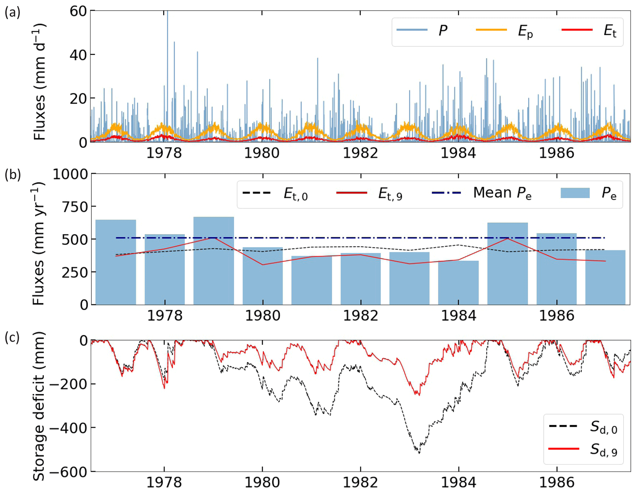
Figure A1Storage deficit iteration approach in a temperate catchment for the time period 1977–1987. (a) Daily water fluxes with P representing precipitation, Ep potential evaporation and Et the initial transpiration calculation based on Eq. (7). (b) Annual water fluxes with Pe representing effective precipitation, Et,0 the initial transpiration estimate and Et,9 the final iteration transpiration estimate. Mean Pe is based on the full time period (1973–2010). (c) Daily storage deficit with Sd,0 representing the initial calculation and Sd,9 the final iteration.
Catchment discharge observations were taken from the Australian Bureau of Meteorology and can be downloaded from http://www.bom.gov.au/water/hrs/ (last access: September 2019) (Australian Government Bureau of Meteorology, 2019). FLUXCOM evaporation data were taken from the FLUXCOM initiative and can be downloaded from http://www.fluxcom.org/EF-Download/ (last access: December 2019) (Jung, 2019). Top-of-atmosphere radiation data were taken from Mines ParisTech and can be downloaded from http://www.soda-pro.com/web-services/radiation/extraterrestrial-irradiance-and-toa/ (last access: September 2019) (Mines ParisTech solar radiation data, 2016). The offline HTESSEL model was provided by EC-EARTH, together with the GSWP-3 forcing data as well as vegetation and soil data. The adapted modules, model output and analysis codes are available upon request. The Python scripts used for Sr calculation and statistical significance of the results can be downloaded from https://github.com/fvanoorschot/Python-scripts-van-Oorschot-2021/ (last access: June 2021) (van Oorschot, 2021).
The supplement related to this article is available online at: https://doi.org/10.5194/esd-12-725-2021-supplement.
The study was conceived by RJvdE and amended with input from all authors. FvO carried out the study, analyzed the results and wrote the paper with input and feedback from RJvdE, MH and AA. Specific knowledge and support for the Sr calculations were provided by MH, and specific knowledge and support for the EC-EARTH model were provided by AA.
The authors declare that they have no conflict of interest.
Publisher's note: Copernicus Publications remains neutral with regard to jurisdictional claims in published maps and institutional affiliations.
Acknowledgement is given for the use of ECMWF's computing and archive facilities for this research, which were provided by the KNMI and by ECMWF in the framework of the special project SPITALES. This work was supported by the European Union's Horizon 2020 research and innovation program under grant agreement no. 101004156 (CONFESS project). Ruud J. van der Ent acknowledges funding from the Netherlands Organization for Scientific Research (NWO) under project number 016.Veni.181.015.
This research has been supported by the Horizon 2020 project (CONFESS project no. 101004156) and the NWO (project no. 016.Veni.181.015).
This paper was edited by Axel Kleidon and reviewed by Andrew Guswa, Stefan Hagemann, and one anonymous referee.
Ardilouze, C., Batté, L., Bunzel, F., Decremer, D., Déqué, M., Doblas-Reyes, F. J., Douville, H., Fereday, D., Guemas, V., MacLachlan, C., Müller, W., and Prodhomme, C.: Multi-model assessment of the impact of soil moisture initialization on mid-latitude summer predictability, Clim. Dynam., 49, 3959–3974, https://doi.org/10.1007/s00382-017-3555-7, 2017. a
Australian Government Bureau of Meteorology: Hydrologic Reference Stations, available at: http://www.bom.gov.au/water/hrs/index.shtml, last access: September 2019. a, b, c, d
Balsamo, G., Viterbo, P., Beijaars, A., van den Hurk, B., Hirschi, M., Betts, A. K., and Scipal, K.: A revised hydrology for the ECMWF model: Verification from field site to terrestrial water storage and impact in the integrated forecast system, J. Hydrometeorol., 10, 623–643, https://doi.org/10.1175/2008JHM1068.1, 2009. a, b, c
Balsamo, G., Pappenberger, F., Dutra, E., Viterbo, P., and van den Hurk, B.: A revised land hydrology in the ECMWF model: a step towards daily water flux prediction in a fully-closed water cycle, Hydrol. Process., 25, 1046–1054, https://doi.org/10.1002/hyp.7808, 2011. a
Bouaziz, L., Weerts, A., Schellekens, J., Sprokkereef, E., Stam, J., Savenije, H., and Hrachowitz, M.: Redressing the balance: quantifying net intercatchment groundwater flows, Hydrol. Earth Syst. Sci., 22, 6415–6434, https://doi.org/10.5194/hess-22-6415-2018, 2018. a
Canadell, J., Jackson, R., Ehleringer, J., Mooney, H., Sala, O., and Schulze, E.-D.: Maximum rooting depth of vegetation types at the global scale, Oecologia, 108, 583–595, https://doi.org/10.1007/BF00329030, 1996. a
Collins, D. B. and Bras, R. L.: Plant rooting strategies in water-limited ecosystems, Water Resour. Res., 43, 1–10, https://doi.org/10.1029/2006WR005541, 2007. a, b
Condon, L. E., Markovich, K. H., Kelleher, C. A., McDonnell, J. J., Ferguson, G., and McIntosh, J. C.: Where Is the Bottom of a Watershed?, Water Resour. Res., 56, e2019WR026010, https://doi.org/10.1029/2019WR026010, 2020. a
De Boer-Euser, T., McMillan, H. K., Hrachowitz, M., Winsemius, H. C., and Savenije, H. H.: Influence of soil and climate on root zone storage capacity, Water Resour. Res., 52, 2009–2024, https://doi.org/10.1002/2015WR018115, 2016. a, b, c, d, e, f
de Rosnay, P. and Polcher, J.: Modelling root water uptake in a complex land surface scheme coupled to a GCM, Hydrol. Earth Syst. Sci., 2, 239–255, https://doi.org/10.5194/hess-2-239-1998, 1998. a
Desborough, C. E.: The impact of root weighting on the response of transpiration to moisture stress in land surface schemes, Mon. Weather Rev., 125, 1920–1930, https://doi.org/10.1175/1520-0493(1997)125<1920:TIORWO>2.0.CO;2, 1997. a
Dümenil, L. and Todini, E.: A rainfall–runoff scheme for use in the Hamburg climate model, in: Advances in Theoretical Hydrology, edited by: O'Kane, J. P., European Geophysical Society Series on Hydrological Sciences, Elsevier, Amsterdam, 129–157, https://doi.org/10.1016/B978-0-444-89831-9.50016-8, 1992. a
ECMWF: Part IV: Physical Processes, IFS Documentation, available at: https://www.ecmwf.int/node/17117 (last access: September 2019), 2016. a, b, c, d, e
Euser, T., Hrachowitz, M., Winsemius, H. C., and Savenije, H. H.: The effect of forcing and landscape distribution on performance and consistency of model structures, Hydrol. Process., 29, 3727–3743, https://doi.org/10.1002/hyp.10445, 2015. a
FAO: Digital Soil Map of the World (DSMW), Tech. rep., Food and Agricultural Organization of the United Nations, re-issued version, 2003. a, b
Feddes, R. A., Hoff, H., Bruen, M., Dawson, T., De Rosnay, P., Dirmeyer, P., Jackson, R. B., Kabat, P., Kleidon, A., Lilly, A., and Pitman, A. J.: Modeling root water uptake in hydrological and climate models, B. Am. Meteorol. Soc., 82, 2797–2809, https://doi.org/10.1175/1520-0477(2001)082<2797:MRWUIH>2.3.CO;2, 2001. a
Ferguson, I. M., Jefferson, J. L., Maxwell, R. M., and Kollet, S. J.: Effects of root water uptake formulation on simulated water and energy budgets at local and basin scales, Environ. Earth Sci., 75, 1–15, https://doi.org/10.1007/s12665-015-5041-z, 2016. a
Gao, H., Hrachowitz, M., Schymanski, S. J., Fenicia, F., Sriwongsitanon, N., and Savenije, H. H. G.: Climate controls how ecosystems size the root zone storage capacity at catchment scale, Geophys. Res. Lett., 41, 7916–7923, https://doi.org/10.1002/2014GL061668, 2014. a, b, c, d, e, f
Gentine, P., D'Odorico, P., Lintner, B. R., Sivandran, G., and Salvucci, G.: Interdependence of climate, soil, and vegetation as constrained by the Budyko curve, Geophys. Res. Lett., 39, 2–7, https://doi.org/10.1029/2012GL053492, 2012. a, b, c
Gerrits, A. M., Pfister, L., and Savenije, H. H.: Spatial and temporal variability of canopy and forest floor interception in a beech forest, Hydrol. Process., 24, 3011–3025, https://doi.org/10.1002/hyp.7712, 2010. a
Gharari, S., Clark, M. P., Mizukami, N., Wong, J. S., Pietroniro, A., and Wheater, H. S.: Improving the Representation of Subsurface Water Movement in Land Models, J. Hydrometeorol., 20, 2401–2418, https://doi.org/10.1175/JHM-D-19-0108.1, 2019. a
Gumbel, E. J.: Les valeurs extrêmes des distributions statistiques, Ann I H Poincaré, 5, 115–158, 1935. a
Guswa, A. J.: The influence of climate on root depth: A carbon cost-benefit analysis, Water Resour. Res., 44, 1–11, https://doi.org/10.1029/2007WR006384, 2008. a, b
Hagemann, S. and Stacke, T.: Impact of the soil hydrology scheme on simulated soil moisture memory, Clim. Dynam., 44, 1731–1750, https://doi.org/10.1007/s00382-014-2221-6, 2015. a
Hargreaves, G. H. and Samani, Z. A.: Estimating potential evapotranspiration, J. Irr. Drain. Div.-ASCE, 108, 225–230, 1982. a
Herwitz, S. R.: Interception storage capacities of tropical rainforest canopy trees, J. Hydrol., 77, 237–252, https://doi.org/10.1016/0022-1694(85)90209-4, 1985. a
Hrachowitz, M., Stockinger, M., Coenders-Gerrits, M., van der Ent, R., Bogena, H., Lücke, A., and Stumpp, C.: Deforestation reduces the vegetation-accessible water storage in the unsaturated soil and affects catchment travel time distributions and young water fractions, Hydrol. Earth Syst. Sci. Discuss. [preprint], https://doi.org/10.5194/hess-2020-293, in review, 2020. a
Jackson, R. B., Canadell, J., Ehleringer, J. R., Mooney, H. A., Sala, O. E., and Schulze, E. D.: A global analysis of root distributions for terrestrial biomes, Oecologia, 108, 389–411, https://doi.org/10.1007/BF00333714, 1996. a
Jeffrey, S. J., Carter, J. O., Moodie, K. B., and Beswick, A. R.: Using spatial interpolation to construct a comprehensive archive of Australian climate data, Environ. Modell. Softw., 16, 309–330, https://doi.org/10.1016/S1364-8152(01)00008-1, 2001. a
Jung, M.: FLUXCOM Energy Fluxes, available at: http://www.fluxcom.org/EF-Download/, last access: December 2019. a
Jung, M., Koirala, S., Weber, U., Ichii, K., Gans, F., Camps-Valls, G., Papale, D., Schwalm, C., Tramontana, G., and Reichstein, M.: The FLUXCOM ensemble of global land-atmosphere energy fluxes, Sci. Data, 6, 74, https://doi.org/10.1038/s41597-019-0076-8, 2019. a, b, c
Kim, H.: Global Soil Wetness Project Phase 3 Atmospheric Boundary Conditions (Experiment 1) [Data set], Data Integration and Analysis System (DIAS), https://doi.org/10.20783/DIAS.501, 2017. a, b
Kleidon, A.: Global datasets of rooting zone depth inferred from inverse methods, J. Climate, 17, 2714–2722, https://doi.org/10.1175/1520-0442(2004)017<2714:GDORZD>2.0.CO;2, 2004. a
Kleidon, A. and Heimann, M.: A method of determining rooting depth from a terrestrial biosphere model and its impacts on the global water and carbon cycle, Glob. Change Biol., 4, 275–286, https://doi.org/10.1046/j.1365-2486.1998.00152.x, 1998. a, b
Ma, N., Szilagyi, J., and Jozsa, J.: Benchmarking large-scale evapotranspiration estimates: A perspective from a calibration-free complementary relationship approach and FLUXCOM, J. Hydrol., 590, 125–221, https://doi.org/10.1016/j.jhydrol.2020.125221, 2020. a
Mahfouf, J. F., Ciret, C., Ducharne, A., Irannejad, P., Noilhan, J., Shao, Y., Thornton, P., Xue, Y., and Yang, Z. L.: Analysis of transpiration results from the RICE and PILPS workshop, Global Planet. Change, 13, 73–88, https://doi.org/10.1016/0921-8181(95)00039-9, 1996. a
Milly, P. C.: Climate, soil water storage, and the average annual water balance, Water Resour. Res., 30, 2143–2156, https://doi.org/10.1029/94WR00586, 1994. a, b
Mines ParisTech solar radiation data: Extraterrestrial irradiance (e0) and top of atmosphere (TOA) radiation, available at: http://www.soda-pro.com/web-services/radiation/extraterrestrial-irradiance-and-toa (last access: September 2019), 2016. a, b
Nijzink, R., Hutton, C., Pechlivanidis, I., Capell, R., Arheimer, B., Freer, J., Han, D., Wagener, T., McGuire, K., Savenije, H., and Hrachowitz, M.: The evolution of root-zone moisture capacities after deforestation: a step towards hydrological predictions under change?, Hydrol. Earth Syst. Sci., 20, 4775–4799, https://doi.org/10.5194/hess-20-4775-2016, 2016. a, b, c
Norby, R. and Jackson, R.: Root dynamics and global change: seeking an ecosystem perspective, New Phytol., 147, 1–2, https://doi.org/10.1046/j.1469-8137.2000.00674.x, 2000. a
Oudin, L., Andréassian, V., Perrin, C., and Anctil, F.: Locating the sources of low-pass behavior within rainfall-runoff models, Water Resour. Res., 40, W11101, https://doi.org/10.1029/2004WR003291, 2004. a
Pan, S., Pan, N., Tian, H., Friedlingstein, P., Sitch, S., Shi, H., Arora, V. K., Haverd, V., Jain, A. K., Kato, E., Lienert, S., Lombardozzi, D., Nabel, J. E. M. S., Ottlé, C., Poulter, B., Zaehle, S., and Running, S. W.: Evaluation of global terrestrial evapotranspiration using state-of-the-art approaches in remote sensing, machine learning and land surface modeling, Hydrol. Earth Syst. Sci., 24, 1485–1509, https://doi.org/10.5194/hess-24-1485-2020, 2020. a, b
Pastorello, G., Trotta, C., Canfora, E., et al.: The FLUXNET2015 dataset and the ONEFlux processing pipeline for eddy covariance data, Sci. Data, 7, 225, https://doi.org/10.1038/s41597-020-0534-3, 2020. a
Pitman, A. J.: The evolution of, and revolution in, land surface schemes designed for climate models, Int. J. Climatol., 23, 479–510, https://doi.org/10.1002/joc.893, 2003. a
Sakschewski, B., von Bloh, W., Drüke, M., Sörensson, A. A., Ruscica, R., Langerwisch, F., Billing, M., Bereswill, S., Hirota, M., Oliveira, R. S., Heinke, J., and Thonicke, K.: Variable tree rooting strategies improve tropical productivity and evapotranspiration in a dynamic global vegetation model, Biogeosciences Discuss. [preprint], https://doi.org/10.5194/bg-2020-97, in review, 2020. a, b
Schenk, H. J. and Jackson, R. B.: Rooting depths, lateral root spreads and below-ground/above-ground allometries of plants in water-limited ecosystems, J. Ecol., 90, 480–494, https://doi.org/10.1046/j.1365-2745.2002.00682.x, 2002a. a, b
Schenk, H. J. and Jackson, R. B.: The Global Biogeography of Roots, Ecol. Monogr., 72, 311–328, https://doi.org/10.1890/0012-9615(2002)072[0311:TGBOR]2.0.CO;2, 2002b. a, b, c
Schlesinger, W. H. and Jasechko, S.: Transpiration in the global water cycle, Agr. Forest Meteorol., 189–190, 115–117, https://doi.org/10.1016/j.agrformet.2014.01.011, 2014. a
Seneviratne, S. I., Koster, R. D., Guo, Z., Dirmeyer, P. A., Kowalczyk, E., Lawrence, D., Liu, P., Lu, C. H., Mocko, D., Oleson, K. W., and Verseghy, D.: Soil moisture memory in AGCM simulations: Analysis of global land-atmosphere coupling experiment (GLACE) data, J. Hydrometeorol., 7, 1090–1112, https://doi.org/10.1175/JHM533.1, 2006. a
Seneviratne, S. I., Corti, T., Davin, E. L., Hirschi, M., Jaeger, E. B., Lehner, I., Orlowsky, B., and Teuling, A. J.: Investigating soil moisture-climate interactions in a changing climate: A review, Earth-Sci. Rev., 99, 125–161, https://doi.org/10.1016/j.earscirev.2010.02.004, 2010. a
Singh, C., Wang-Erlandsson, L., Fetzer, I., Rockström, J., and van der Ent, R.: Rootzone storage capacity reveals drought coping strategies along rainforest-savanna transitions, Environ. Res. Lett., 15, 124021, https://doi.org/10.1088/1748-9326/abc377, 2020. a, b
Sivandran, G. and Bras, R. L.: Dynamic root distributions in ecohydrological modeling: A case study at Walnut Gulch Experimental Watershed, Water Resour. Res., 49, 3292–3305, https://doi.org/10.1002/wrcr.20245, 2013. a
Teuling, A. J., Seneviratne, S. I., Williams, C., and Troch, P. A.: Observed timescales of evapotranspiration response to soil moisture, Geophys. Res. Lett., 33, L23403, https://doi.org/10.1029/2006GL028178, 2006. a
van den Hurk, B. and Viterbo, P.: The Torne-Kalix PILPS 2 (e) experiment as a test bed for modifications to the ECMWF land surface scheme, Global Planet. Change, 38, 165–173, 2003. a
van den Hurk, B., Viterbo, P., Beljaars, A., and Betts, A.: Offline validation of the ERA40 surface scheme, https://doi.org/10.21957/9aoaspz8, 2000. a
van den Hurk, B., Kim, H., Krinner, G., Seneviratne, S. I., Derksen, C., Oki, T., Douville, H., Colin, J., Ducharne, A., Cheruy, F., Viovy, N., Puma, M. J., Wada, Y., Li, W., Jia, B., Alessandri, A., Lawrence, D. M., Weedon, G. P., Ellis, R., Hagemann, S., Mao, J., Flanner, M. G., Zampieri, M., Materia, S., Law, R. M., and Sheffield, J.: LS3MIP (v1.0) contribution to CMIP6: the Land Surface, Snow and Soil moisture Model Intercomparison Project – aims, setup and expected outcome, Geosci. Model Dev., 9, 2809–2832, https://doi.org/10.5194/gmd-9-2809-2016, 2016. a
Van Genuchten, M. T.: A closed-form equation for predicting the hydraulic conductivity of unsaturated soils 1, Soil Sci. Soc. Am. J., 44, 892–898, https://doi.org/10.2136/sssaj1980.03615995004400050002x, 1980. a
van Oorschot, F.: fvanoorschot/Python-scripts-van-Oorschot-2021, Github, available at: https://github.com/fvanoorschot/Python-scripts-van-Oorschot-2021/, last access: June 2021. a
Wang-Erlandsson, L., Bastiaanssen, W. G. M., Gao, H., Jägermeyr, J., Senay, G. B., van Dijk, A. I. J. M., Guerschman, J. P., Keys, P. W., Gordon, L. J., and Savenije, H. H. G.: Global root zone storage capacity from satellite-based evaporation, Hydrol. Earth Syst. Sci., 20, 1459–1481, https://doi.org/10.5194/hess-20-1459-2016, 2016. a, b, c, d, e
Wartenburger, R., Seneviratne, S. I., Hirschi, M., Chang, J., Ciais, P., Deryng, D., Elliott, J., Folberth, C., Gosling, S. N., Gudmundsson, L., Henrot, A.-J., Hickler, T., Ito, A., Khabarov, N., Kim, H., Leng, G., Liu, J., Liu, X., Masaki, Y., Morfopoulos, C., Müller, C., Schmied, H. M., Nishina, K., Orth, R., Pokhrel, Y., Pugh, T. A. M., Satoh, Y., Schaphoff, S., Schmid, E., Sheffield, J., Stacke, T., Steinkamp, J., Tang, Q., Thiery, W., Wada, Y., Wang, X., Weedon, G. P., Yang, H., and Zhou, T.: Evapotranspiration simulations in ISIMIP2a–Evaluation of spatio-temporal characteristics with a comprehensive ensemble of independent datasets, Environ. Res. Lett., 13, 075001, https://doi.org/10.1088/1748-9326/aac4bb, 2018. a
Zeng, X., Dai, Y. J., Dickinson, R. E., and Shaikh, M.: The role of root distribution for climate simulation over land, Geophys. Res. Lett., 25, 4533–4536, https://doi.org/10.1029/1998GL900216, 1998. a, b