Jarzynski equality and Crooks relation for local models of air–sea interaction

We show that the most prominent of the work theorems, the Jarzynski equality and the Crooks relation, can be applied to the momentum transfer at the air–sea interface using a hierarchy of local models. In the more idealized models, with and without a Coriolis force, the variability is provided from Gaussian white noise which modifies the shear between the atmosphere and the ocean. The dynamics is Gaussian, and the Jarzynski equality and Crooks relation can be obtained analytically solving stochastic differential equations. The more involved model consists of interacting atmospheric and oceanic boundary layers, where only the dependence on the vertical direction is resolved, the turbulence is modeled through standard turbulent models and the stochasticity comes from a randomized drag coefficient. It is integrated numerically and can give rise to a non-Gaussian dynamics. Also in this case the Jarzynski equality allows for calculating a dynamic beta β_D of the turbulent fluctuations (the equivalent of the thermodynamic beta $\mathit{\beta }=(k_{\mathrm{B}}T{)}^{-\mathrm{1}}$ in thermal fluctuations). The Crooks relation gives the β_D as a function of the magnitude of the work fluctuations. It is well defined (constant) in the Gaussian models and can show a slight variation in the more involved models. This demonstrates that recent concepts of stochastic thermodynamics used to study micro-systems subject to thermal fluctuations can further the understanding of geophysical fluid dynamics with turbulent fluctuations.

1 Introduction

To better understand the interactions between different components of the climate system is an important and difficult task. The problem lies in the different science proper to each component leading to disparate processes, evolving on dissimilar scales in space and time. This heterogeneity complexifies the research, from an observational, theoretical and numerical perspective. Air–sea interaction is one example. The exchange of heat, momentum and matter between the atmosphere and the ocean has a strong influence on our climate (Stocker et al., 2007). In the present work only the exchange of momentum is considered. It is caused by the shear at the sea surface due to the difference between the atmospheric winds and the ocean currents in the corresponding planetary boundary layers. For a general discussion on air–sea interaction we refer to Csanady (2001). The atmospheric winds are usually faster than the ocean currents, and therefore the atmosphere mostly loses energy at the interface by friction and the ocean mostly gains energy (e.g., Wirth, 2019). The energy exchange is not conservative, and most of the energy is dissipated (Duhaut and Straub, 2006; Wirth, 2018).

Since the work of Einstein (1906) (see also Einstein, 1956; Perrin, 2014), fluctuations have been the focus of research in statistical mechanics, which had traditionally been concerned with averages. Fluctuations in a thermodynamic system usually appear at spatial scales which are small enough so that thermal, molecular motion leaves an imprint on the dynamics, as was first noted by Einstein (1906) (see also Einstein, 1956; Perrin, 2014). The importance of fluctuations is, however, not restricted to small systems where thermal fluctuations are important, since they leave their imprint on the dynamics at all scales when (not necessarily thermal) fluctuations are strong enough. A typical example of non-thermal fluctuations is fluctuating turbulent fluid motion (e.g., Frisch, 1995). The average motion of a turbulent fluid can not be understood without some knowledge about the turbulent fluctuations. The importance of turbulent fluctuations is especially pronounced in geophysical flows, which are highly anisotropic due to the influence of gravity. This leads to a quasi-two-dimensional dynamics, an energy cascade from small to large scales and strong fluctuations (see Boffetta and Ecke, 2012, for a recent review on 2D turbulence). Likewise, the air–sea interaction on hourly to climatic timescales can not be understood without some knowledge of the fluctuations at smaller and faster scales (see McWilliams and Huckle, 2006; Shrira and Almelah, 2020). Furthermore, in many natural systems the focus is on the fluctuations rather than on an average state. Examples are weather and climate dynamics, where we focus on the fluctuations in the same system on different timescales. For the weather the timescale of interest is from roughly an hour to a week; for the climate the focus is from tens to thousands of years. As processes with very different timescales intervene, the system is not in a stationary state at those timescales but is constantly evolving in time. The different components of the system exchange energy; they do work on each other. The exchange of energy between fluctuating components is the subject of the present work.

A recent concept, which is presently the subject of attention when non-equilibrium thermal systems are considered, are work theorems. The most prominent ones are the Jarzynski equality (Jarzynski, 1997) and the Crooks relation (Crooks, 1998). Rather than looking at average values of the thermodynamic variables, they consider their probability density functions (pdf's) which allow the replacement of inequalities of equilibrium statistical mechanics by equalities. As an example, the second law of thermodynamics states that the work W performed on a system is larger than or equal to the increase ΔG in its free energy: W≥ΔG. When the work is seen as a fluctuating quantity w, which differs even when a specific process is repeated with the same deterministic forcing protocol but is subject to thermal fluctuations, the Jarzynski equality says that $\langle \exp (-\mathit{\beta }w)\rangle =\exp (-\mathit{\beta }\mathrm{\Delta }G)$, where the average 〈〉 is taken over the ensemble of thermal fluctuations. This not only includes the second law on average but also says that individual exceptions have to exist (see Sect. 2). When thermal fluctuations are considered, the (thermodynamic) $\mathit{\beta }=(k_{\mathrm{B}}T{)}^{-\mathrm{1}}$ is the inverse of the product of the Boltzmann constant and the temperature. In the case of air–sea interaction, considered here, the dynamic β, (denoted β_D) is the inverse of an energy related to the macroscopic turbulent fluctuations. It is the inverse of a “temperature”, that is, in the present context, of a turbulent kinetic energy.

The here discussed work theorems are different but related to fluctuation theorems considered in Wirth (2018, 2019). In a recent review Seifert (2012) presents the relation of fluctuation theorems, the Jarzynski equality, the Crooks relation and other recent concepts of non-equilibrium thermodynamics and develops a unifying framework. Work theorems are considered based on different approaches: Hamiltonian dynamics subject to an external forcing, Fokker–Planck equations and Langevin dynamics (see Seifert, 2012, for a review). Here only the last approach is used.

The concepts developed for micro-dynamics with fluctuations due to thermal motion are here applied to macroscopic fluid dynamics, where an atmospheric planetary boundary layer interacts with an oceanic mixed layer. In this case the fluctuations are due to the smaller-scale turbulence in both layers. The concepts of fluctuation theorems have been previously applied to cases with turbulent rather than thermal fluctuations. Examples are the experimental data of the drag force exerted by a turbulent flow (Ciliberto et al., 2004) and the local entropy production in Rayleigh–Bénard convection (Shang et al., 2005).

A system that is subject to an external forcing typically evolves in time; it is in a non-stationary state. If there is a balance between external forcings and/or internal dissipation in such a way that ensemble averages do not evolve in time, the system is in a non-equilibrium stationary state. In the here-considered work theorems a dissipative system is subject to forcing and also the average large-scale quantities evolve in time; the dynamics is in a non-stationary non-equilibrium state.

The concepts of non-equilibrium statistical mechanics have been applied to momentum transfer between the atmosphere and the ocean in a non-rotating frame in Wirth (2018, 2019). This was done by adapting the mathematics developed to study the movement of a Brownian particle. The present work prolongs this research by considering work relations and extending it to the dynamics in a rotating frame. The motion of a particle in a rotating frame is similar to Brownian motion of a charged particle in a magnetic field, a problem which has been studied since Taylor (1961) (see also Czopnik and Garbaczewski, 2001). The structure of the equations is identical when the Larmor frequency of a charged particle in a magnetic field is replaced by the Coriolis frequency. The passage from a non-rotating frame to a rotating frame is, however, far from straightforward, for principally two reasons. First, the dynamics is no longer invariant by time reversal, even in the non-dissipative limit. In the words of statistical mechanics, detailed balance, which is the basis of many analytical results, is lost. Secondly, it is not clear that results from simple models that do not explicitly resolve the vertical structure in the atmospheric and oceanic boundary layer are useful to investigate the situation in a rotating frame with a Coriolis force (see McWilliams and Huckle, 2006). Indeed, the dynamics in the planetary boundary layer shows a strong dependence on the vertical coordinate, not only in magnitude but also in direction as determined by Ekman (1905). Analytic solutions for time evolution are only available in special cases (see Shrira and Almelah, 2020). In the present pedagogical approach to the subject we therefore work with a hierarchy of three models. The first model is a linear zero-dimensional one-component model (1D velocity vector). We analytically prove the validity of the work theorems by solving the corresponding stochastic differential equation (SDE). In the second model the Coriolis force is added, and it has two horizontal components (2D velocity vector). The work theorems are again proven analytically. The third model is a fully non-linear model, explicitly resolving the vertical dependence of the interacting atmospheric and oceanic boundary layer, which is integrated numerically.

In the next section we introduce the theory of stochastic thermodynamics and work relations applied to air–sea interaction. The models are introduced and solved, using stochastic calculus, in Sect. 3. As the concepts are new to the field (see Ghil, 2019, for a historical perspective), we present all the calculations in detail for pedagogical purposes and also to show that most of it reduces to linear algebra. We refer the reader not familiar with stochastic differential equations to Dijkstra (2013) and Franzke et al. (2015). The results, for the three models of our model hierarchy, are discussed in Sect. 4, and we end with some conclusions in Sect. 5.

2 Theory

2.1 Model

2.1.1 The 1D two-component model (1D2C)

We consider the turbulent momentum transfer between the atmospheric and the oceanic planetary boundary layer, which are coupled by a frictional force. The atmospheric layer is also subject to a deterministic forcing imposed from the exterior through a pressure gradient. The dynamics in the boundary layers is investigated using Reynolds decomposition, in which the fast fluctuations in the three-dimensional velocity are separated from the slowly evolving component of the horizontal velocity field (called “velocity field” in the sequel). The horizontal variations in the velocity field are neglected. This is justified in a local model by the disparity of the vertical and horizontal scales. The atmospheric planetary boundary layer is a few hundreds of meters thick. The oceanic planetary boundary layer spans a few tens of meters in the vertical. The velocity field in both layers varies considerably over the thickness of the corresponding boundary layer. Horizontal variations are imposed by the weather systems that force the dynamics and typically extend 1000 km in the horizontal. This leads to a classical model of the planetary boundary layers (introduced by Ekman, 1905), which depends on the vertical direction (1D) and resolves the two horizontal components (2C) of the velocity vector ${\stackrel{\mathrm{̃}}{\mathbf{u}}}_{\mathrm{a}}(z,t)=\left({\stackrel{\mathrm{̃}}{u}}_{\mathrm{a}}\right(z,t),{\stackrel{\mathrm{̃}}{v}}_{\mathrm{a}}(z,t\left)\right)$¹; this 1D2C model is given by an evolution equation of both velocity components:

$$\begin{array}{}\text{(1a)}& {\displaystyle }{\partial }_t{\stackrel{\mathrm{̃}}{u}}_{\mathrm{a}}(z,t)=f{\stackrel{\mathrm{̃}}{v}}_{\mathrm{a}}(z,t)+{\partial }_z\left[{\mathit{\nu }}_{\mathrm{a}}\right(z,t\left){\partial }_z{\stackrel{\mathrm{̃}}{u}}_{\mathrm{a}}\right(z,t\left)\right]+{\stackrel{\mathrm{̃}}{F}}_x\left(t\right),\text{(1b)}& {\displaystyle }{\partial }_t{\stackrel{\mathrm{̃}}{v}}_{\mathrm{a}}(z,t)=-f{\stackrel{\mathrm{̃}}{u}}_{\mathrm{a}}(z,t)+{\partial }_z\left[{\mathit{\nu }}_{\mathrm{a}}\right(z,t\left){\partial }_z{\stackrel{\mathrm{̃}}{v}}_{\mathrm{a}}\right(z,t\left)\right]+{\stackrel{\mathrm{̃}}{F}}_y\left(t\right),\end{array}$$

where f is the Coriolis frequency; ν_a(z,t) the turbulent viscosity; and $\stackrel{\mathrm{̃}}{\mathbf{F}}=({\stackrel{\mathrm{̃}}{F}}_x,{\stackrel{\mathrm{̃}}{F}}_y)$ a forcing provided by a large-scale pressure gradient, which is independent of the vertical direction. The turbulent viscosity ν_a(z,t) parameterizes the effect of the not-explicitly-resolved fluctuations on the velocity field; it is calculated through a turbulent closure scheme. The atmosphere extends over $z\in [\mathrm{0},h_{\mathrm{a}}]$, and the boundary conditions are (Neumann at top and bottom)

$$\begin{array}{}\text{(2a)}& {\displaystyle }({\partial }_z{\stackrel{\mathrm{̃}}{\mathbf{u}}}_{\mathrm{a}}{)}_{z=h_{\mathrm{a}}}=\mathrm{0},\text{(2b)}& {\displaystyle }({\mathit{\nu }}_{\mathrm{a}}{\partial }_z{\stackrel{\mathrm{̃}}{\mathbf{u}}}_{\mathrm{a}}{)}_{z=\mathrm{0}}={\displaystyle \frac{\mathit{\tau }}{{\mathit{\rho }}_{\mathrm{a}}}},\end{array}$$

where ρ_a is a constant atmospheric density. The ocean is also governed by model (Eq. 1) where all subscripts are changed (_a→_o); the forcing vanishes; the domain extends over $z\in [-h_{\mathrm{o}},\mathrm{0}]$; and the boundary conditions are (Neumann at bottom and top)

$$\begin{array}{}\text{(3a)}& {\displaystyle }({\partial }_z{\stackrel{\mathrm{̃}}{\mathbf{u}}}_{\mathrm{o}}{)}_{z=-h_{\mathrm{o}}}=\mathrm{0},\text{(3b)}& {\displaystyle }({\mathit{\nu }}_{\mathrm{o}}{\partial }_z{\stackrel{\mathrm{̃}}{\mathbf{u}}}_{\mathrm{o}}{)}_{z=\mathrm{0}}={\displaystyle \frac{\mathit{\tau }}{{\mathit{\rho }}_{\mathrm{o}}}}.\end{array}$$

The surface friction $\mathit{\tau }=({\mathit{\tau }}_y,{\mathit{\tau }}_y)$ is parameterized as a function of the velocity difference between the atmospheric and oceanic velocity near the interface z=0. Linear Rayleigh friction (i.e., parameterized to be linearly proportional to the relative wind) is employed:

$$\begin{array}{}\text{(4)}& \mathit{\tau }={\mathit{\rho }}_{\mathrm{o}}{h}_{\mathrm{o}}S\left({\stackrel{\mathrm{̃}}{\mathbf{u}}}_{\mathrm{a}}\right({\mathit{\delta }}_{\mathrm{a}})-{\stackrel{\mathrm{̃}}{\mathbf{u}}}_{\mathrm{o}}(-{\mathit{\delta }}_{\mathrm{o}}\left)\right).\end{array}$$

Here S⁻¹ is oceanic friction time, or a quadratic drag law:

$$\begin{array}{}\text{(5)}& \mathit{\tau }={\mathit{\rho }}_{\mathrm{o}}{c}_{\mathrm{d}}\left|{\stackrel{\mathrm{̃}}{\mathbf{u}}}_{\mathrm{a}}\right({\mathit{\delta }}_{\mathrm{a}})-{\stackrel{\mathrm{̃}}{\mathbf{u}}}_{\mathrm{o}}(-{\mathit{\delta }}_{\mathrm{o}}\left)\right|\left({\stackrel{\mathrm{̃}}{\mathbf{u}}}_{\mathrm{a}}\right({\mathit{\delta }}_{\mathrm{a}})-{\stackrel{\mathrm{̃}}{\mathbf{u}}}_{\mathrm{o}}(-{\mathit{\delta }}_{\mathrm{o}}\left)\right),\end{array}$$

with δ_a≪h_a and δ_o≪h_o. Here the drag coefficient c_d is defined relative to the ocean and the equivalent drag coefficient for the atmosphere is obtained by multiplying c_d by ${\mathit{\rho }}_{\mathrm{o}}/{\mathit{\rho }}_{\mathrm{a}}$.

2.1.2 The 0D two-component model (0D2C)

The 0D version of the 1D2C model (Eq. 1) is obtained by integration over the vertical extent of the corresponding layer normalized by the layer thickness. Introducing

$$\begin{array}{}\text{(6)}& \begin{array}{r}{\mathbf{u}}_{\mathrm{a}}=(u_{\mathrm{a}},v_{\mathrm{a}})={\displaystyle \frac{\mathrm{1}}{h_{\mathrm{a}}}}\underset{\mathrm{0}}{\overset{h_{\mathrm{a}}}{\int }}{\stackrel{\mathrm{̃}}{\mathbf{u}}}_{\mathrm{a}}\left(z\right)\mathrm{d}z,\\ {\mathbf{u}}_{\mathrm{o}}=(u_{\mathrm{o}},v_{\mathrm{o}})={\displaystyle \frac{\mathrm{1}}{h_{\mathrm{o}}}}\underset{-h_{\mathrm{o}}}{\overset{\mathrm{0}}{\int }}{\stackrel{\mathrm{̃}}{\mathbf{u}}}_{\mathrm{o}}\left(z\right)\mathrm{d}z\end{array}\end{array}$$

and using the boundary conditions (Eqs. 2 and 3) as well as the linear Rayleigh friction (Eq. 4), we obtain the following 0D2C model for the atmosphere:

$$\begin{array}{}\text{(7a)}& {\displaystyle }{\partial }_t{u}_{\mathrm{a}}=f{v}_{\mathrm{a}}-mS(u_{\mathrm{a}}-u_{\mathrm{o}})+F_x,\text{(7b)}& {\displaystyle }{\partial }_t{v}_{\mathrm{a}}=-f{u}_{\mathrm{a}}-mS(v_{\mathrm{a}}-v_{\mathrm{o}})+F_y,\end{array}$$

where $m=\frac{{\mathit{\rho }}_{\mathrm{o}}{h}_{\mathrm{o}}}{{\mathit{\rho }}_{\mathrm{a}}{h}_{\mathrm{a}}}$ is the mass ratio between the oceanic layer and the atmospheric layer and $\mathbf{F}\left(t\right)=(F_x,F_y)$ is analogous to $\stackrel{\mathrm{̃}}{\mathbf{F}}\left(t\right)$. Similarly for the ocean, we have

$$\begin{array}{}\text{(8a)}& {\displaystyle }{\partial }_t{u}_{\mathrm{o}}=f{v}_{\mathrm{o}}+S(u_{\mathrm{a}}-u_{\mathrm{o}}),\text{(8b)}& {\displaystyle }{\partial }_t{v}_{\mathrm{o}}=-f{u}_{\mathrm{o}}+S(v_{\mathrm{a}}-v_{\mathrm{o}}).\end{array}$$

The upper ocean is mainly forced at its surface by the wind shear. Forcing due to the dynamics of the deeper or surrounding ocean is not considered by the model. The momentum exchange between the layers due to unresolved turbulent motion is parameterized by a random force $\mathit{\zeta }=({\mathit{\zeta }}_x,{\mathit{\zeta }}_y)$, added to the friction law. The model under consideration in the following thus reads

$$\begin{array}{}\text{(9a)}& {\displaystyle }{\partial }_t{u}_{\mathrm{a}}=f{v}_{\mathrm{a}}-mS(u_{\mathrm{a}}-u_{\mathrm{o}})+F_x+{\displaystyle \frac{m}{M}}{\mathit{\zeta }}_x,\text{(9b)}& {\displaystyle }{\partial }_t{v}_{\mathrm{a}}=-f{u}_{\mathrm{a}}-mS(v_{\mathrm{a}}-v_{\mathrm{o}})+F_y+{\displaystyle \frac{m}{M}}{\mathit{\zeta }}_y,\text{(9c)}& {\displaystyle }{\partial }_t{u}_{\mathrm{o}}=-f{v}_{\mathrm{o}}+S(u_{\mathrm{a}}-u_{\mathrm{o}})-{\displaystyle \frac{\mathrm{1}}{M}}{\mathit{\zeta }}_x,\text{(9d)}& {\displaystyle }{\partial }_t{v}_{\mathrm{o}}=-f{u}_{\mathrm{o}}+S(v_{\mathrm{a}}-v_{\mathrm{o}})-{\displaystyle \frac{\mathrm{1}}{M}}{\mathit{\zeta }}_y,\end{array}$$

where the stochastic noise has been scaled by $M=m+\mathrm{1}$ to simplify the algebra in the following. Note that M is the total mass per unit surface. The analytical solution to the coupled model (Eq. 9) is given in Appendix B. When the Coriolis parameter vanishes (f=0) and the linear friction law is used, the dynamics in the two horizontal directions is uncoupled. In this case a simple 0D1C model can be obtained by setting v_a to 0 in Eq. (9a) (or v_o=0 in Eq. 9c) and discarding Eq. (9b) (or Eq. 9d).

Let us also introduce the integrated mode, which gives the momentum integrated over $[-h_{\mathrm{o}},h_{\mathrm{a}}]$, and the shear mode:

$$\begin{array}{}\text{(10a)}& {\displaystyle }{\mathbf{u}}_I={\mathbf{u}}_{\mathrm{a}}+m{\mathbf{u}}_{\mathrm{o}},\text{(10b)}& {\displaystyle }{\mathbf{u}}_S={\mathbf{u}}_{\mathrm{a}}-{\mathbf{u}}_{\mathrm{o}}.\end{array}$$

The shear and the turbulence in the atmosphere and the ocean do not affect the integrated momentum u_I. The two layers only interact by friction, which acts as a damping on the shear mode (see Sects. A1 and B1). The only remaining two parameters in the problem are the constant mass ratio of the oceanic versus the atmospheric layer, m, and the function S. For the case of linear Rayleigh friction (Eq. 4), S is constant. When the turbulent, quadratic friction law (Eq. 5) applies, we have $S=c_{\mathrm{d}}\left|{\mathbf{u}}_S\right|/h_{\mathrm{o}}$, with a constant drag coefficient c_D.

The departures from the vertical average in the atmosphere and the ocean are given by

$$\begin{array}{}\text{(11a)}& {\displaystyle }{\mathbf{u}}_{\mathrm{a}}^{\prime }\left(z\right)={\stackrel{\mathrm{̃}}{\mathbf{u}}}_{\mathrm{a}}\left(z\right)-{\mathbf{u}}_{\mathrm{a}},\text{(11b)}& {\displaystyle }{\mathbf{u}}_{\mathrm{o}}^{\prime }\left(z\right)={\stackrel{\mathrm{̃}}{\mathbf{u}}}_{\mathrm{o}}\left(z\right)-{\mathbf{u}}_{\mathrm{o}}.\end{array}$$

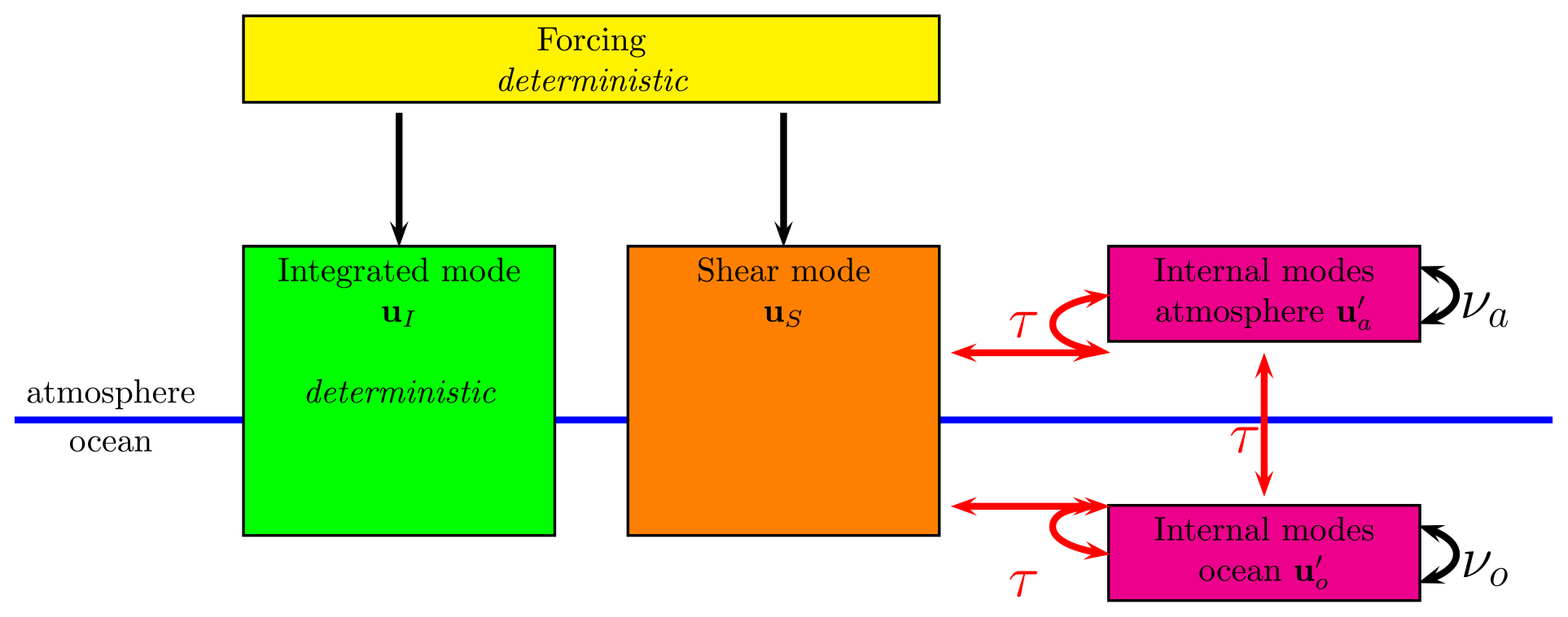
Figure 1 Schematic of the models considered: the integrated mode and the shear mode are forced. The integrated mode is decoupled from the rest of the dynamics. The shear mode is coupled to the internal modes of the atmosphere and the ocean by the surface stress. The internal modes in the atmosphere and the ocean depend on the eddy viscosity in each layer and the surface stress. The randomness arises through the surface friction τ (red color). In the 1D model the internal dynamics in the atmospheric and oceanic layer are explicitly resolved and random noise is added to the surface friction coefficient. In the 0D model their influence on the shear mode is parameterized by random noise.

The interaction between the different components is schematized in Fig. 1. The dynamics of the integrated mode, u_I, does not depend on the shear τ, as can be verified when Eq. (10a) is combined with Eq. (9) (see Sects. A1and B1). Newton's laws insure that the dynamics of the integrated mode is independent of the interior dynamics, that is of u_S, ${\mathbf{u}}_{\mathrm{a}}^{\prime }$, ${\mathbf{u}}_{\mathrm{o}}^{\prime }$, ν_a(z) and ν_o(z). This property is lost when a dependence on the horizontal directions is included. Due to the boundary conditions, it is also not subject to dissipation and therefore conserves its (kinetic) energy. The dynamics of the integrated mode is purely deterministic, and the work W_I done on it equals the increase in the free energy ΔG. The shear mode u_S interacts with the internal modes in the atmosphere, ${\mathbf{u}}_{\mathrm{a}}^{\prime }$, and the ocean, ${\mathbf{u}}_{\mathrm{o}}^{\prime }$, through the shear at the interface τ. The dynamics in the shear mode does not depend explicitly on the internal viscosity ν_a(z) and ν_o(z) in the two layers but only through ${\mathbf{u}}_{\mathrm{a}}^{\prime }$ and ${\mathbf{u}}_{\mathrm{o}}^{\prime }$. As ${\mathbf{u}}_{\mathrm{a}}^{\prime }$ has a vanishing vertical average, it is not forced by the pressure gradient. The dynamics of ${\mathbf{u}}_{\mathrm{a}}^{\prime }$ depends explicitly on u_S, ${\mathbf{u}}_{\mathrm{a}}^{\prime }$, ${\mathbf{u}}_{\mathrm{o}}^{\prime }$ and ν_a(z). The same applies to the ocean. In the 0D models the effect of the internal modes (magenta boxes in Fig. 1) on the shear mode is modeled by a stochastic noise. In the 1D model the internal dynamics is resolved explicitly; stochastic noise is added to the drag coefficient only and enters the dynamics through the shear at the interface (red arrows in Fig. 1); see Sect. 3.3 for more details on this point. Looking at air–sea interaction in terms of modes not only is a technical simplification but also emphasizes the view of seeing the atmosphere and the ocean as a combined system rather than as separate atmospheric and oceanic layers that act on each other. From Eqs. (10a) and (10b) we easily obtain that

$$\begin{array}{}\text{(12a)}& {\displaystyle }{\mathbf{u}}_{\mathrm{a}}={\displaystyle \frac{\mathrm{1}}{M}}({\mathbf{u}}_I+m{\mathbf{u}}_S),\text{(12b)}& {\displaystyle }{\mathbf{u}}_{\mathrm{o}}={\displaystyle \frac{\mathrm{1}}{M}}({\mathbf{u}}_I-{\mathbf{u}}_S),\end{array}$$

with $M=m+\mathrm{1}$ being the total mass per unit surface.

2.2 Stochastic thermodynamics

The concept of stochastic thermodynamics was introduced by Sekimoto (1998) (see also Seifert, 2012). Rather than considering the classical dynamics described by Hamilton's equations over the entire phase space of all microstates, on one hand, or the averaged thermodynamic quantities, without internal dynamics, on the other, it takes an intermediate position by looking at mesostates (also called statistical states). A mesostate does not completely determine the microstate of the system but represents an ensemble of microstates. It is therefore not described by a sharp value but by a pdf. Its mathematical framework comprises the Langevin equation and the stochastic differential equations, which describe the evolution of a pdf. It is a dynamics with a deterministic and stochastic part that interact. Such an approach is adapted when external forces only constrain part of the dynamics as the internal response of the system is too involved (chaotic or turbulent), so it can only be described in a stochastic sense. If a specific force is applied to a system, the outcome depends on the initial microstate that is usually not precisely known and its evolution has a random component. By considering the evolution of the pdf, which takes into account the uncertainty in the microstates that influences the system, we obtain a deterministic evolution of the pdf.

We here apply these concepts to air–sea interaction; the “heat”, the source of the fluctuation, in our approach is (small-scale) turbulent motion, all that is represented in magenta and red in Fig. 1. The macroscopic variable are the slowly varying vertically averaged velocities u_a and u_o or equivalently modes u_I and u_S. In analogy to the first law of thermodynamics we write

$$\begin{array}{}\text{(13)}& \mathrm{d}W=\mathrm{d}V-\mathrm{d}Q.\end{array}$$

The work applied to the system by the external force $\mathbf{F}=(F_x,F_y)$ in Eq. (9) is

$$\begin{array}{}\text{(14)}& \mathrm{d}W=\mathbf{F}\cdot \mathrm{d}{\mathbf{x}}_{\mathrm{a}}=\mathbf{F}\cdot {\mathbf{u}}_{\mathrm{a}}\mathrm{d}t.\end{array}$$

For the sake of readability, in the sequel we will omit the dot symbol “⋅” in vector products. V, dV and dQ should be understood as scalar quantities in the following. The internal (kinetic) energy is

$$\begin{array}{}\text{(15)}& {\displaystyle }V={\displaystyle \frac{\mathrm{1}}{\mathrm{2}}}({\mathbf{u}}_{\mathrm{a}}^{\mathrm{2}}+m{\mathbf{u}}_{\mathrm{o}}^{\mathrm{2}})={\displaystyle \frac{\mathrm{1}}{\mathrm{2}M}}({\mathbf{u}}_I^{\mathrm{2}}+m{\mathbf{u}}_S^{\mathrm{2}}),\text{(16)}& {\displaystyle }dV={\mathbf{u}}_{\mathrm{a}}d{\mathbf{u}}_{\mathrm{a}}+m{\mathbf{u}}_{\mathrm{o}}d{\mathbf{u}}_{\mathrm{o}}={\displaystyle \frac{\mathrm{1}}{M}}({\mathbf{u}}_I\mathrm{d}{\mathbf{u}}_I+m{\mathbf{u}}_S\mathrm{d}{\mathbf{u}}_S),\end{array}$$

and the heat provided to the system (Q<0 as friction dissipates heat) is

$$\begin{array}{}\text{(17)}& \begin{array}{rl}\mathrm{d}Q& =\mathrm{d}V-\mathrm{d}W={\mathbf{u}}_{\mathrm{a}}\mathrm{d}{\mathbf{u}}_{\mathrm{a}}+m{\mathbf{u}}_{\mathrm{o}}\mathrm{d}{\mathbf{u}}_{\mathrm{o}}-{\mathbf{Fu}}_{\mathrm{a}}\mathrm{d}t\\ & ={\displaystyle \frac{\mathrm{1}}{M}}({\mathbf{u}}_I\mathrm{d}{\mathbf{u}}_I+m{\mathbf{u}}_S\mathrm{d}{\mathbf{u}}_S)-\mathbf{F}{\displaystyle \frac{\mathrm{1}}{M}}({\mathbf{u}}_I+m{\mathbf{u}}_S)\mathrm{d}t.\end{array}\end{array}$$

The dissipation to heat is given by

$$\begin{array}{}\text{(18)}& \begin{array}{rl}{\displaystyle \frac{\mathrm{d}Q}{\mathrm{d}t}}& ={\mathbf{u}}_{\mathrm{a}}{\displaystyle \frac{d{\mathbf{u}}_{\mathrm{a}}}{\mathrm{d}t}}+m{\mathbf{u}}_{\mathrm{o}}{\displaystyle \frac{d{\mathbf{u}}_{\mathrm{o}}}{\mathrm{d}t}}-{\mathbf{Fu}}_{\mathrm{a}}={\mathbf{u}}_{\mathrm{a}}(-Sm{\mathbf{u}}_{\mathrm{a}}+Sm{\mathbf{u}}_{\mathrm{o}}\\ & +\mathbf{F})+m{\mathbf{u}}_{\mathrm{o}}(-S{\mathbf{u}}_{\mathrm{o}}+S{\mathbf{u}}_{\mathrm{a}})-{\mathbf{Fu}}_{\mathrm{a}}=-Sm({\mathbf{u}}_{\mathrm{a}}-{\mathbf{u}}_{\mathrm{o}}{)}^{\mathrm{2}}\\ & =-Sm{\mathbf{u}}_S^{\mathrm{2}}.\end{array}\end{array}$$

To derive the second line we used Eqs. (9a–9d). The shear force between the layers is Su_S; when the friction law is linear S is a constant; otherwise it is a function of the shear. Furthermore if we consider a process that starts at A and finishes at B, we have

$$\begin{array}{}\text{(19)}& \begin{array}{rl}W(A\to B)& =\underset{x\left(A\right)}{\overset{x\left(B\right)}{\int }}\mathbf{F}\mathrm{d}{\mathbf{x}}_{\mathrm{a}}=\underset{t\left(A\right)}{\overset{t\left(B\right)}{\int }}\mathbf{F}{\mathbf{u}}_{\mathrm{a}}\mathrm{d}t\\ & ={\displaystyle \frac{\mathrm{1}}{M}}\underset{t\left(A\right)}{\overset{t\left(B\right)}{\int }}\mathbf{F}({\mathbf{u}}_I+m{\mathbf{u}}_S)\mathrm{d}t.\end{array}\end{array}$$

The free energy is $\mathrm{\Delta }G=V\left(\mathrm{\infty }\right)-V\left(A\right)=\frac{\mathrm{1}}{\mathrm{2}M}{\mathbf{u}}_I^{\mathrm{2}}$, the energy in the integrated mode, as the energy in the shear mode is dissipated away in time. The energy in the integrated mode changes only when a forcing is applied, so it varies only when the protocol A→B, or its inverse, is applied, whereas the internal energy V varies before and after. Note that $\frac{\mathrm{d}Q}{\mathrm{d}t}<\mathrm{0}$, and therefore $\mathrm{\Delta }G<W(A\to B)$ and $-\mathrm{\Delta }G<W(B\to A)$, which leads to $-W(B\to A)<\mathrm{\Delta }G<W(A\to B)$. This means that more work than the free energy has to be provided to go from A to B and less work than the free energy is recuperated on the reverse (conjugated) path. In a cyclic process B=A, ΔG=0 and all the work injected into the system is ultimately dissipated.

It is important to note that the Coriolis parameter does not explicitly appear in the equation of the work or the heat as the Coriolis force is orthogonal to the local velocity. However, the Coriolis parameter strongly influences the dynamics, that is u_a and u_o. Through this influence, it has a determining role on the work and heat budget.

2.3 Forward, inverse and reverse processes

The forcing protocol on the time interval [0,T] is given by

$$\begin{array}{}\text{(20)}& {{\stackrel{\mathrm{̃}}{\mathbf{F}}}^f}_{A\to B}\left(t\right)=\mathbf{F}\left(t\right),\end{array}$$

where the function F has a compact support within the interval [0,T], It is important to note that even if the system evolves (relaxes) outside the interval [0,T], no work is performed on the system as the force is vanishing. When the Coriolis force is present, the system is generally not in a stationary state after the forcing but performs inertial oscillations. To bring the system back to the initial state, an inverse protocol has to be performed at precisely a multiple of the inertial period after the forward protocol:

$$\begin{array}{}\text{(21)}& {{\stackrel{\mathrm{̃}}{\mathbf{F}}}^i}_{B\to A}\left(t\right)=-\mathbf{F}(t-{\displaystyle \frac{\mathrm{2}\mathit{\pi }}{f}}n),n\in \mathbb{N}.\end{array}$$

For a reverse protocol it is required that the forcing is

$$\begin{array}{}\text{(22)}& {{\stackrel{\mathrm{̃}}{\mathbf{F}}}^r}_{B\to A}\left(t\right)=-\mathbf{F}(T-t+t_{\mathrm{0}}).\end{array}$$

To satisfy both conditions we impose the symmetries

$$\begin{array}{}\text{(23)}& \mathbf{F}(T/\mathrm{2}-t)=\mathbf{F}(T/\mathrm{2}+t)\mathrm{and}{t}_{\mathrm{0}}={\displaystyle \frac{\mathrm{2}\mathit{\pi }}{f}}n,n\in \mathbb{N}.\end{array}$$

If we neglect the turbulence in both layers, which is modeled by a stochastic term, the dynamics is deterministic. During the forward process, starting from rest and applying the protocol ${\stackrel{\mathrm{̃}}{\mathbf{F}}}_{A\to B}\left(t\right)$, we have

$$\begin{array}{}\text{(24)}& {\displaystyle }{\mathbf{u}}_I^f\left(\mathrm{0}\right)={\mathbf{u}}_S^f\left(\mathrm{0}\right)=\mathrm{0}\to {\mathbf{u}}_I^f\left(T\right),{\mathbf{u}}_S^f\left(\mathrm{\infty }\right)=\mathrm{0},\text{(25)}& {\displaystyle }\mathrm{\Delta }{G}^f\left(\mathrm{\infty }\right)=\mathrm{\Delta }G,W^f=\mathrm{\Delta }G+Q^f,Q^f(\mathrm{0},\mathrm{\infty })=Q.\end{array}$$

The reverse process starts from the converged state, is forced by ${{\stackrel{\mathrm{̃}}{\mathbf{F}}}^r}_{B\to A}\left(t\right)$ for a period T and then relaxes to rest at t=∞:

$$\begin{array}{}\text{(26)}& {\displaystyle }{\mathbf{u}}_I^r\left(\mathrm{0}\right)={\mathbf{u}}_I^f\left(T\right),{\mathbf{u}}_S^r\left(\mathrm{0}\right)=\mathrm{0}\to {\mathbf{u}}_I^r\left(T\right),{\mathbf{u}}_S^r\left(\mathrm{\infty }\right)=\mathrm{0},\text{(27)}& {\displaystyle }\mathrm{\Delta }{G}^r\left(\mathrm{\infty }\right)=-\mathrm{\Delta }G,W^r=-\mathrm{\Delta }G+Q^r,Q^r(\mathrm{0},\mathrm{\infty })=Q.\end{array}$$

Note that $-W^r\le \mathrm{\Delta }G\le W^f$ which is a statement of the second law of thermodynamics. When the process is reversible then the equalities apply. Furthermore we always have $\mathrm{2}\mathrm{\Delta }G=W^f-W^r$. So far the dynamics considered has been deterministic.

The turbulent motion within the system is due to internal dynamics and is modeled by stochastic terms. When noise is added in the linear model, it does not interfere with the deterministic dynamics but simply adds to it. Furthermore, the force is deterministic, so the randomness in the work is provided solely by the fluctuations in u_a. As randomness resides only in the shear mode, the fluctuations in the work $w^{\prime }=m{\int }_{\mathrm{0}}^T{\mathbf{Fu}}_S^{\prime }\mathrm{d}t$ come from fluctuations in the shear mode ${\mathbf{u}}_S^{\prime }$. Note that the vertical average of ${\mathbf{u}}_{\mathrm{a}}^{\prime }$ vanishes, so the internal modes do not contribute to the work. When the noise terms are Gaussian and the friction linear, the velocities are Gaussian variables and so is the work performed on the layers and modes. The average of these variables are given by the deterministic part (〈w^f〉=W^f and 〈w^r〉=W^r), and the variance ${\mathit{\sigma }}_W^{\mathrm{2}}\left(T\right)$ is obtained through the variance of the shear mode. In the case with an internal turbulent dynamics, $-W^r\le \mathrm{\Delta }{G}^f\left(\mathrm{\infty }\right)\le W^f$ is true for averages only; individual trajectories can be exceptions.

In the Gaussian case the pdf's for the forward and reverse processes are

$$\begin{array}{}\text{(28)}& {\displaystyle }{\mathrm{pdf}}^f\left(w\right)={\displaystyle \frac{\mathrm{1}}{\sqrt{\mathrm{2}\mathit{\pi }}{\mathit{\sigma }}_W}}\exp \left(-{\displaystyle \frac{(w-W^f{)}^{\mathrm{2}}}{\mathrm{2}{\mathit{\sigma }}_W^{\mathrm{2}}}}\right),\text{(29)}& {\displaystyle }{\mathrm{pdf}}^r\left(w\right)={\displaystyle \frac{\mathrm{1}}{\sqrt{\mathrm{2}\mathit{\pi }}{\mathit{\sigma }}_W}}\exp \left(-{\displaystyle \frac{(w-W^r{)}^{\mathrm{2}}}{\mathrm{2}{\mathit{\sigma }}_W^{\mathrm{2}}}}\right).\end{array}$$

Note that the pdf's are identical except for a shift of 2ΔG^f(∞) in z. Examples of the pdf's in the Gaussian case for the forward and reverse processes, as well as of the pdf's of the reverse process flipped at the origin, are shown, for different values of the work averages and β_D, in the schematic Fig. 2 for illustration.

2.4 Jarzynski equality

We denote the averaging with respect to the forward process by

$$\begin{array}{}\text{(30)}& \langle X\left(w\right){\rangle }_f=\underset{-\mathrm{\infty }}{\overset{\mathrm{\infty }}{\int }}X\left(w\right){\mathrm{pdf}}^f\left(w\right)\mathrm{d}w.\end{array}$$

The Jarzynski equality is then expressed by

$$\begin{array}{}\text{(31)}& \langle e^{-\mathit{\beta }w}{\rangle }_f=e^{-\mathit{\beta }\mathrm{\Delta }G}.\end{array}$$

In the Gaussian case we have

$$\begin{array}{}\text{(32)}& \langle e^{-\mathit{\beta }w}{\rangle }_f={\displaystyle \frac{\mathrm{1}}{\sqrt{\mathrm{2}\mathit{\pi }}{\mathit{\sigma }}_W}}\underset{-\mathrm{\infty }}{\overset{\mathrm{\infty }}{\int }}{e}^{-\mathit{\beta }w}\exp (-{\displaystyle \frac{(w-W^f{)}^{\mathrm{2}}}{\mathrm{2}{\mathit{\sigma }}_W^{\mathrm{2}}}})\mathrm{d}w,\end{array}$$

and verifying the Jarzynski equality reduces to equating the powers of the exponential:

$$\begin{array}{}\text{(33)}& -(w-W^f{)}^{\mathrm{2}}-\mathrm{2}\mathit{\beta }{\mathit{\sigma }}_W^{\mathrm{2}}(w-\mathrm{\Delta }G)=-(w-W_{\mathrm{0}}{)}^{\mathrm{2}}.\end{array}$$

The only non-trivial solution is

$$\begin{array}{}\text{(34)}& \mathit{\beta }={\displaystyle \frac{\mathrm{2}Q}{{\mathit{\sigma }}_w^{\mathrm{2}}}}\mathrm{and}{W}_{\mathrm{0}}=W^r.\end{array}$$

The Jarzynski equality applies when β is a constant, independent of the forcing protocol F and T. At first sight Eq. (34) is astonishing, as the Jarzynski equality expressed by Eq. (31) seems to be a statement on the free energy which solely depends on the integrated mode. Equation (34), however, connects the heat dissipated in the shear mode to the work fluctuations, which are only due to the shear mode. Furthermore, we have seen that the dynamics of the two modes are unrelated. This apparent inconsistency is resolved by multiplying Eq. (31) by e^βΔG on both sides. It is then apparent that an average of the exponential of ΔG−w is taken, which only depends on the shear mode. Note that when thermal fluctuations are considered, ${\mathit{\beta }}^{-\mathrm{1}}=k_{\mathrm{B}}T$ and more generally for the Ornstein–Uhlenbeck process, with an auto-correlation of the noise characterized by the variable R (defined below through Eq. 40), ${\mathit{\beta }}_{\mathrm{D}}^{-\mathrm{1}}=\frac{R}{\mathrm{SM}}$, which relates the fluctuations to the dissipation and shows the connection of the Jarzynski equality to the fluctuation dissipation relation and the fluctuation dissipation theorem (see Wirth, 2019, 2018).

Experiments can also be performed for different values of β_D (see the schematic Fig. 2). If the turbulence level decreases, β_D increases and the dynamics converges towards a deterministic process. Note that neither ΔG−W nor ${\mathit{\sigma }}_w^{\mathrm{2}}$ depends on u_I(0); in the case of vanishing Coriolis force this is equivalent to Galilean invariance.

Furthermore, neither the work nor the free energy depends on the relaxation process and in an experiment it is not necessary to wait for the relaxation to the stationary state to obtain the free energy. It is only necessary to repeat the experiment sufficiently many times to obtain statistically significant results and use the Jarzynski equality to obtain the free energy. The work does, however, depend on u_S(0), and so we have to start from equilibrium (〈u_S(0)〉=0 and $\langle {\mathbf{u}}_S(\mathrm{0}{)}^{\mathrm{2}}\rangle ={\mathit{\beta }}_{\mathrm{D}}^{-\mathrm{1}}$). The Jarzynski equality also shows that, as ${\mathit{\sigma }}_w^{\mathrm{2}}>\mathrm{0}$, there have to be (rare) paths for which the work performed is smaller than the free energy. This is easily seen as $e^{-x}<\mathrm{1}$ for x>0. In thermodynamics these paths are sometimes referred to as “violations of the second law of thermodynamics”. The probability of such a violation occurring in the Gaussian case can be expressed using the error function as $\mathrm{erf}\left(\right(\mathrm{\Delta }G-W^f)/{\mathit{\sigma }}_W))$. However, due to the convexity of the exponential function 〈e^x〉≥e^〈x〉 (called Jensen's inequality), and therefore 〈w〉≥ΔG and the second law of thermodynamics is verified in an average sense, it is a statistical law.

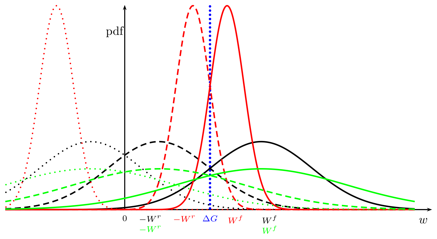
Figure 2 The pdf's of the forward (pdf^f(w), solid lines), the backward (pdf^r(w), dotted lines) and the negative of the backward (pdf^r(−w), dashed lines) processes are shown. The averages W^f and −W^r are given on the horizontal axis for the processes. The red line represents an experiment that was performed at a slower rate; less work is provided on average, and fluctuations are smaller as compared to the experiment corresponding to the black line. The green line represents an experiment that was performed at a lower dynamic β_D as compared to the experiment corresponding to the black line; averages agree, but fluctuations are higher. The dotted lines are shifted by 2ΔG to the left with respect to the solid lines of the same color. The solid lines and the dashed lines of the same color all intersect at w=ΔG and the dotted lines, and the dashed lines of the same color all intersect at w=0. For an experiment performed at β_D=∞ (zero temperature) or an experiment performed at an infinitely slow rate T→∞, all the pdf's are the delta function δ(w−ΔG) (blue line) and the dynamics is deterministic.

2.5 Crooks relation

The Jarzynski equality (JE) considers an average with respect to the forward process, whereas the Crooks relation (CR) compares the pdf's of the forward and reverse process, without any averaging; it states

$$\begin{array}{}\text{(35)}& {\displaystyle \frac{{\mathrm{pdf}}^f\left(w\right)}{{\mathrm{pdf}}^r(-w)}}=\exp \left({\mathit{\beta }}_{\mathrm{D}}\right[w-\mathrm{\Delta }G\left]\right)=\exp (-{\mathit{\beta }}_{\mathrm{D}}q).\end{array}$$

where $q=\mathrm{\Delta }G-w$ is the negative dissipation along a single trajectory with work w and Q=〈q〉 by definition. The CR is also useful to determine ΔG; it is the value w where the graphs of the forward pdf and the reverse pdf of the negative argument cross, where pdf^f(w) is pdf^r(−w) (see Fig. 2). When the shapes of the forward and reverse pdf agree, the free energy can be also obtained via ${\mathrm{pdf}}^r\left(w\right)={\mathrm{pdf}}^f(w+\mathrm{2}\mathrm{\Delta }G)$. The first method is useful when β_D is small, and the second is useful when it is large. The CR considers the pdf, and the JE which is concerned with averages can be derived from it through dividing Eq. (35) by exp (β_Dq) multiplying by pdf^r(−w) and integrating over w from −∞ to ∞. In cyclic or stationary processes the free energy gain is vanishing, the reverse pdf equals the forward pdf and the CR simplifies to the detailed fluctuation theorem.

In the Gaussian case described above the CR is obtained by a straightforward calculation:

$$\begin{array}{}\text{(36)}& \begin{array}{rl}{\displaystyle \frac{{\mathrm{pdf}}^f\left(w\right)}{{\mathrm{pdf}}^r(-w)}}& =\exp \left({\displaystyle \frac{\mathrm{1}}{\mathrm{2}{\mathit{\sigma }}_w^{\mathrm{2}}}}\right(-w^{\mathrm{2}}+\mathrm{2}{W}^{f}w-(W^f{)}^{\mathrm{2}}+w^{\mathrm{2}}\\ & +\mathrm{2}{W}^{r}w+\left(W^r{)}^{\mathrm{2}}\right))=\exp ({\mathit{\beta }}_{\mathrm{D}}[w-\mathrm{\Delta }G])\\ & =\exp (-{\mathit{\beta }}_{\mathrm{D}}q).\end{array}\end{array}$$

2.6 Integral fluctuation theorem

Note also that when the CR holds,

$$\begin{array}{}\text{(37)}& \mathrm{1}={〈{\displaystyle \frac{{\mathrm{pdf}}^r(-w)}{{\mathrm{pdf}}^f\left(w\right)}}〉}_f=\langle \exp \left({\mathit{\beta }}_{\mathrm{D}}q\right){\rangle }_f.\end{array}$$

This is the integral fluctuation theorem; it shows that there exists trajectories with q>0, demonstrating violations of the second law of thermodynamics. It is proven by using Jensen's inequality: $\mathrm{1}=\langle \exp \left({\mathit{\beta }}_{\mathrm{D}}q\right)\rangle \ge \exp \left({\mathit{\beta }}_{\mathrm{D}}Q\right)$, which leads to Q≥0. The integral fluctuation theorem is a reformulation of the JE in terms of dissipated heat.

In cyclic or stationary processes the free energy gain vanishes. When a force is applied, it typically drives the system and does work, which is dissipated to heat. Rare events when the work is negative and heat does work must exist, following the derived results above.

3 Results

The work relations are investigated for a hierarchy of models of air–sea interaction. This not only favors a pedagogical discussion of the subject but also helps to emphasize critical points in the application of the theory exposed above. The simpler models, which are given by Eq. (9), are called 0D models as the variables have no spatial dependence. The friction force between the two layers is parameterized by linear Rayleigh friction, which allows for analytical solutions. In these linear models which are subject to Gaussian noise (through the ζ_x and ζ_y terms in Eq. 9 the pdf's of the work are Gaussian random variables, which are determined by their mean, their variance and their temporal correlation). In this case the work theorems are algebraic relations between the means and the variances which can be calculated analytically using stochastic calculus. The first model of interest, referred to as 0D1C model, does not include the Coriolis force (f=0), and the dynamics in the two horizontal directions (the two components of the velocity vector) are independent. The analytical solution for this model is given in Sect. 3.1. The 0D1C model represents the simplest example in which work theorems can be discussed and solved analytically by employing Newton's laws and solving stochastic differential equations. It can also be shown that in this case the work theorems are a consequence of Galilean invariance. When the Coriolis force is added the 0D2C model (Eq. 9) is recovered and the dynamics in the two horizontal directions interact. The Coriolis force also adds several conceptual difficulties to the problem. First, for Brownian motion of particles subject to a Coriolis force, detailed balance is lost as the dynamics is not time reversible. Second, Galilean invariance is broken, even for the deterministic part of the problem. Third, the application of a reverse protocol depends on the timing. The same force can increase or reduce the free energy depending on when, at which phase, it is applied. We calculate the work theorem analytically by employing Newton's laws and solving stochastic differential equations in Sect. 3.2.

We then discuss in Sect. 3.3 a non-linear model with a vertical dependence on the atmosphere and ocean (1D2C model) that describes the non-linear interaction of the two planetary boundary layers. It is described by Eqs. (1), (2), (3) and (5). The model is deterministic except for the drag coefficient, which has a stochastic part. All results concerning this model are obtained through numerical integration of the corresponding governing equations.

3.1 The linear 0D1C model

The solution of the 0D1C model introduced in Sect. 2.1 is

$$\begin{array}{}\text{(38a)}& {\displaystyle }\begin{array}{rl}{u}_{\mathrm{a}}\left(t\right)& =u_{\mathrm{a}}\left(\mathrm{0}\right)-\left(u_{\mathrm{a}}\right(\mathrm{0})-u_{\mathrm{o}}(\mathrm{0}\left)\right){\displaystyle \frac{m}{M}}\left(\mathrm{1}-e^{-MSt}\right)\\ & +\underset{\mathrm{0}}{\overset{t}{\int }}{\displaystyle \frac{\mathrm{1}}{M}}\left(\mathrm{1}+m{e}^{-MS(t-t^{\prime })}\right)\mathcal{F}\left(t^{\prime }\right)\mathrm{d}{t}^{\prime }\\ & +{\displaystyle \frac{m}{M}}\underset{\mathrm{0}}{\overset{t}{\int }}{e}^{-MS(t-t^{\prime })}\mathit{\zeta }\left(t^{\prime }\right)\mathrm{d}{t}^{\prime },\end{array}\text{(38b)}& {\displaystyle }\begin{array}{rl}{u}_{\mathrm{o}}\left(t\right)& =u_{\mathrm{o}}\left(\mathrm{0}\right)+\left(u_{\mathrm{a}}\right(\mathrm{0})-u_{\mathrm{o}}(\mathrm{0}\left)\right){\displaystyle \frac{\mathrm{1}}{M}}\left(\mathrm{1}-e^{-MSt}\right)\\ & +\underset{\mathrm{0}}{\overset{t}{\int }}{\displaystyle \frac{\mathrm{1}}{M}}\left(\mathrm{1}-e^{-MS(t-t^{\prime })}\right)\mathcal{F}\left(t^{\prime }\right)\mathrm{d}{t}^{\prime }\\ & -{\displaystyle \frac{\mathrm{1}}{M}}\underset{\mathrm{0}}{\overset{t}{\int }}{e}^{-MS(t-t^{\prime })}\mathit{\zeta }\left(t^{\prime }\right)\mathrm{d}{t}^{\prime },\end{array}\end{array}$$

where ℱ(t) is the deterministic forcing of the synoptic atmosphere and ζ a random force. The steps to obtain such solution are given in Sect. A1. In terms of the integrated mode and the shear mode, the equivalent solution is

$$\begin{array}{}\text{(39a)}& {\displaystyle }{u}_I\left(t\right)=\underset{\mathrm{0}}{\overset{t}{\int }}\mathcal{F}\left(t^{\prime }\right)\mathrm{d}t+u_I\left(\mathrm{0}\right),\text{(39b)}& {\displaystyle }{u}_S\left(t\right)=\underset{\mathrm{0}}{\overset{t}{\int }}{e}^{-\mathrm{SM}(t-t^{\prime })}\left[\mathcal{F}\right(t^{\prime })+\mathit{\zeta }(t^{\prime }\left)\right]\mathrm{d}{t}^{\prime }+u_S\left(\mathrm{0}\right)e^{-\mathrm{SM}t}.\end{array}$$

In the following we consider that the noise ζ(t) is delta correlated in time:

$$\begin{array}{}\text{(40)}& \langle \mathit{\zeta }\left(t\right)\mathit{\zeta }\left(t^{\prime }\right)\rangle =\mathrm{2}R\mathit{\delta }(t-t^{\prime }),\end{array}$$

with R being a positive scalar.

3.1.1 Constant forcing

The simplest case is a constant force ℱ(t) of amplitude ℱ₀ during the interval $I=[\mathrm{0},T]$; such forcing satisfies the symmetry required for a reverse protocol as given by Eq. (22). Note that in a linear model the results obtained with such forcing are general because every forcing can be approximated by a sum of step-function forcings or an integral of infinitesimal step functions. The dynamics of a sum of step functions or an integral is the sum or integral of the dynamics of the individual forcings. The solution for $\mathrm{0}\le t\le T$ is

$$\begin{array}{}\text{(41)}& {\displaystyle }{u}_I\left(t\right)={\mathcal{F}}_{\mathrm{0}}t+u_I\left(\mathrm{0}\right),\text{(42)}& {\displaystyle }{u}_S\left(t\right)={\displaystyle \frac{{\mathcal{F}}_{\mathrm{0}}}{\mathrm{SM}}}(\mathrm{1}-e^{-\mathrm{SM}t})+u_S\left(\mathrm{0}\right)e^{-\mathrm{SM}t},\end{array}$$

and for t≥T, it is

$$\begin{array}{}\text{(43)}& {\displaystyle }{u}_I\left(t\right)=u_I\left(T\right),\text{(44)}& {\displaystyle }\begin{array}{rl}{u}_S\left(t\right)& =u_S\left(T\right)e^{-\mathrm{SM}(t-T)}={\displaystyle \frac{{\mathcal{F}}_{\mathrm{0}}}{\mathrm{SM}}}\left(e^{-\mathrm{SM}(t-T)}-e^{-\mathrm{SM}t}\right)\\ & +u_S\left(\mathrm{0}\right)e^{-\mathrm{SM}t}.\end{array}\end{array}$$

The work can be separated in the work done on the shear mode W_S and on the integrated mode W_I. The work the system absorbs as well as how much is absorbed by each mode depends on the state of the system and on the initial condition. The work is

$$\begin{array}{}\text{(45)}& {\displaystyle }\begin{array}{rl}W& =\underset{\mathrm{0}}{\overset{T}{\int }}\mathcal{F}{u}_{\mathrm{a}}\mathrm{d}t=W_S+W_I=\underset{\mathrm{0}}{\overset{T}{\int }}{\displaystyle \frac{\mathcal{F}}{M}}(m{u}_S+u_I)\mathrm{d}t\\ & ={\displaystyle \frac{{\mathcal{F}}_{\mathrm{0}}^{\mathrm{2}}}{\mathrm{2}M}}{T}^{\mathrm{2}}+{\displaystyle \frac{{\mathcal{F}}_{\mathrm{0}}}{M}}\left(u_I\left(\mathrm{0}\right)+{\displaystyle \frac{m{\mathcal{F}}_{\mathrm{0}}}{\mathrm{SM}}}\right)T+{\displaystyle \frac{m{\mathcal{F}}_{\mathrm{0}}}{{\mathrm{SM}}^{\mathrm{2}}}}\\ & \left(u_S\left(\mathrm{0}\right)-{\displaystyle \frac{{\mathcal{F}}_{\mathrm{0}}}{\mathrm{SM}}}\right)(\mathrm{1}-e^{-\mathrm{SM}T}),\end{array}\text{(46)}& {\displaystyle }{W}_I={\displaystyle \frac{{\mathcal{F}}_{\mathrm{0}}^{\mathrm{2}}}{\mathrm{2}M}}{T}^{\mathrm{2}}+{\displaystyle \frac{{\mathcal{F}}_{\mathrm{0}}}{M}}{u}_I\left(\mathrm{0}\right)T,\text{(47)}& {\displaystyle }\begin{array}{rl}{W}_S& ={\displaystyle \frac{m{\mathcal{F}}_{\mathrm{0}}^{\mathrm{2}}}{S^{\mathrm{2}}{M}^{\mathrm{3}}}}(\mathrm{SM}T-\mathrm{1}+e^{-\mathrm{SM}T})+{\displaystyle \frac{m{\mathcal{F}}_{\mathrm{0}}}{{\mathrm{SM}}^{\mathrm{2}}}}\\ & (\mathrm{1}-e^{-\mathrm{SM}T})u_S\left(\mathrm{0}\right).\end{array}\end{array}$$

The kinetic energy is

$$\begin{array}{}\text{(48)}& {\displaystyle }\begin{array}{rl}V\left(T\right)& ={\displaystyle \frac{\mathrm{1}}{\mathrm{2}}}(u_{\mathrm{a}}^{\mathrm{2}}+m{u}_{\mathrm{o}}^{\mathrm{2}})={\displaystyle \frac{\mathrm{1}}{\mathrm{2}M}}(u_I^{\mathrm{2}}+m{u}_S^{\mathrm{2}})\\ & ={\displaystyle \frac{\mathrm{1}}{\mathrm{2}M}}\left(\right({\mathcal{F}}_{\mathrm{0}}T+u_I\left(\mathrm{0}\right){)}^{\mathrm{2}}+m\left({\displaystyle \frac{{\mathcal{F}}_{\mathrm{0}}}{\mathrm{SM}}}\right(\mathrm{1}-e^{-\mathrm{SM}T})\\ & +u_S\left(\mathrm{0}\right)e^{-\mathrm{SM}T}{)}^{\mathrm{2}}),\end{array}\text{(49)}& {\displaystyle }\begin{array}{rl}V\left(t\right)& ={\displaystyle \frac{\mathrm{1}}{\mathrm{2}M}}\left(({\mathcal{F}}_{\mathrm{0}}T+u_I(\mathrm{0}){)}^{\mathrm{2}}\right.\\ & \left.+m{\left({\displaystyle \frac{{\mathcal{F}}_{\mathrm{0}}}{\mathrm{SM}}}(e^{-\mathrm{SM}(t-T)}-e^{-\mathrm{SM}t})+u_S\left(\mathrm{0}\right)e^{-\mathrm{SM}t}\right)}^{\mathrm{2}}\right)\end{array}\end{array}$$

for t>T; if t∈I, replace T with t in the above equation.

The energy difference is

$$\begin{array}{}\text{(50)}& {\displaystyle }\begin{array}{rl}\mathrm{\Delta }V\left(T\right)& =V\left(T\right)-V\left(\mathrm{0}\right)\\ & ={\displaystyle \frac{\mathrm{1}}{\mathrm{2}M}}(u_I^{\mathrm{2}}+m{u}_S^{\mathrm{2}})={\displaystyle \frac{\mathrm{1}}{\mathrm{2}M}}\left(\right({\mathcal{F}}_{\mathrm{0}}T+u_I\left(\mathrm{0}\right){)}^{\mathrm{2}}-u_I(\mathrm{0}{)}^{\mathrm{2}}\\ & +m{\left({\displaystyle \frac{{\mathcal{F}}_{\mathrm{0}}}{\mathrm{SM}}}+\left(u_S\right(\mathrm{0})-{\displaystyle \frac{{\mathcal{F}}_{\mathrm{0}}}{\mathrm{SM}}})e^{-\mathrm{SM}T}\right)}^{\mathrm{2}}-m{u}_S\left(\mathrm{0}{)}^{\mathrm{2}}\right)\\ & ={\displaystyle \frac{{\mathcal{F}}_{\mathrm{0}}^{\mathrm{2}}}{\mathrm{2}M}}{T}^{\mathrm{2}}+{\displaystyle \frac{{\mathcal{F}}_{\mathrm{0}}{u}_I\left(\mathrm{0}\right)}{M}}T+{\displaystyle \frac{m}{\mathrm{2}M}}{\left({\displaystyle \frac{{\mathcal{F}}_{\mathrm{0}}}{\mathrm{SM}}}\right)}^{\mathrm{2}}\\ & +{\displaystyle \frac{m{\mathcal{F}}_{\mathrm{0}}}{{\mathrm{SM}}^{\mathrm{2}}}}\left(u_S\left(\mathrm{0}\right)-{\displaystyle \frac{{\mathcal{F}}_{\mathrm{0}}}{\mathrm{SM}}}\right)e^{-\mathrm{SM}T}\\ & +{\displaystyle \frac{m}{\mathrm{2}M}}{\left(u_S\left(\mathrm{0}\right)-{\displaystyle \frac{{\mathcal{F}}_{\mathrm{0}}}{\mathrm{SM}}}\right)}^{\mathrm{2}}{e}^{-\mathrm{2}\mathrm{SM}T}-{\displaystyle \frac{m}{\mathrm{2}M}}{u}_S(\mathrm{0}{)}^{\mathrm{2}},\end{array}\text{(51)}& {\displaystyle }\mathrm{\Delta }V\left(\mathrm{\infty }\right)={\displaystyle \frac{{\mathcal{F}}_{\mathrm{0}}^{\mathrm{2}}{T}^{\mathrm{2}}}{\mathrm{2}M}}+{\displaystyle \frac{{\mathcal{F}}_{\mathrm{0}}T{u}_I\left(\mathrm{0}\right)}{M}}-{\displaystyle \frac{m}{\mathrm{2}M}}{u}_S(\mathrm{0}{)}^{\mathrm{2}}.\end{array}$$

The free energy is the energy difference in the integrated mode, as the shear mode relaxes to zero in equilibrium, when the forcing has subsided. Therefore it equals the work performed on the integrated mode W_I.

$$\begin{array}{}\text{(52)}& \mathrm{\Delta }G\left(T\right)={\displaystyle \frac{{\mathcal{F}}_{\mathrm{0}}^{\mathrm{2}}{T}^{\mathrm{2}}}{\mathrm{2}M}}+{\displaystyle \frac{{\mathcal{F}}_{\mathrm{0}}T{u}_I\left(\mathrm{0}\right)}{M}}=W_I\end{array}$$

The free energy only varies when work is performed on the system. When the process is infinitely slow, the free energy equals the work. The energy dissipated is

$$\begin{array}{}\text{(53)}& {\displaystyle }\begin{array}{rl}Q(\mathrm{0},T)& =\mathrm{SM}{\displaystyle \frac{m}{M}}\underset{\mathrm{0}}{\overset{T}{\int }}{u}_S^{\mathrm{2}}\mathrm{d}{t}^{\prime }=Sm\underset{\mathrm{0}}{\overset{T}{\int }}\left({\displaystyle \frac{{\mathcal{F}}_{\mathrm{0}}}{\mathrm{SM}}}(\mathrm{1}-e^{-\mathrm{SM}{t}^{\prime }}\right)\\ & +u_S\left(\mathrm{0}\right)e^{-\mathrm{SM}{t}^{\prime }}{)}^{\mathrm{2}}\mathrm{d}{t}^{\prime }\\ & =Sm\left({\left({\displaystyle \frac{{\mathcal{F}}_{\mathrm{0}}}{\mathrm{SM}}}\right)}^{\mathrm{2}}T+{\displaystyle \frac{\mathrm{2}{\mathcal{F}}_{\mathrm{0}}}{(\mathrm{SM}{)}^{\mathrm{2}}}}\left({\displaystyle \frac{{\mathcal{F}}_{\mathrm{0}}}{\mathrm{SM}}}-u_S\left(\mathrm{0}\right)\right)\right.\\ & (e^{-\mathrm{SM}T}-\mathrm{1})\\ & -{\displaystyle \frac{\mathrm{1}}{\mathrm{2}\mathrm{SM}}}({\displaystyle \frac{{\mathcal{F}}_{\mathrm{0}}}{\mathrm{SM}}}-u_S(\mathrm{0}\left){)}^{\mathrm{2}}\right(e^{-\mathrm{2}\mathrm{SM}T}-\mathrm{1}\left)\right)\\ & ={\displaystyle \frac{m{\mathcal{F}}_{\mathrm{0}}^{\mathrm{2}}}{{\mathrm{SM}}^{\mathrm{2}}}}T-{\displaystyle \frac{\mathrm{2}m{\mathcal{F}}_{\mathrm{0}}}{{\mathrm{SM}}^{\mathrm{2}}}}\left(u_S\left(\mathrm{0}\right)-{\displaystyle \frac{{\mathcal{F}}_{\mathrm{0}}}{\mathrm{SM}}}\right)(e^{-\mathrm{SM}T}-\mathrm{1})\\ & -{\displaystyle \frac{m}{\mathrm{2}M}}{\left(u_S\left(\mathrm{0}\right)-{\displaystyle \frac{{\mathcal{F}}_{\mathrm{0}}}{\mathrm{SM}}}\right)}^{\mathrm{2}}(e^{-\mathrm{2}\mathrm{SM}T}-\mathrm{1})\\ & ={\displaystyle \frac{m{\mathcal{F}}_{\mathrm{0}}^{\mathrm{2}}}{{\mathrm{SM}}^{\mathrm{2}}}}T-{\displaystyle \frac{\mathrm{2}m{\mathcal{F}}_{\mathrm{0}}}{{\mathrm{SM}}^{\mathrm{2}}}}\left(u_S\left(\mathrm{0}\right)-{\displaystyle \frac{{\mathcal{F}}_{\mathrm{0}}}{\mathrm{SM}}}\right)e^{-\mathrm{SM}T}\\ & -{\displaystyle \frac{m}{\mathrm{2}M}}{\left(u_S\left(\mathrm{0}\right)-{\displaystyle \frac{{\mathcal{F}}_{\mathrm{0}}}{\mathrm{SM}}}\right)}^{\mathrm{2}}{e}^{-\mathrm{2}\mathrm{SM}T}+{\displaystyle \frac{m{u}_S(\mathrm{0}{)}^{\mathrm{2}}}{\mathrm{2}M}}\\ & -{\displaystyle \frac{\mathrm{3}m{\mathcal{F}}_{\mathrm{0}}^{\mathrm{2}}}{\mathrm{2}{S}^{\mathrm{2}}{M}^{\mathrm{3}}}}+{\displaystyle \frac{m{\mathcal{F}}_{\mathrm{0}}{u}_S\left(\mathrm{0}\right)}{{\mathrm{SM}}^{\mathrm{2}}}},\end{array}\text{(54)}& {\displaystyle }\begin{array}{rl}Q(T,t)& =Sm\underset{T}{\overset{t}{\int }}{u}_S(T{)}^{\mathrm{2}}{e}^{-\mathrm{2}\mathrm{SM}{t}^{\prime }}\mathrm{d}{t}^{\prime }\\ & ={\displaystyle \frac{m{u}_S(T{)}^{\mathrm{2}}}{\mathrm{2}M}}(\mathrm{1}-e^{-\mathrm{2}\mathrm{SM}t}).\end{array}\end{array}$$

3.1.2 Forward and reverse process (deterministic)

The free energy starting from rest is

$$\begin{array}{}\text{(55)}& \mathrm{\Delta }G={\displaystyle \frac{{\mathcal{F}}_{\mathrm{0}}^{\mathrm{2}}{T}^{\mathrm{2}}}{\mathrm{2}M}}.\end{array}$$

The forward process starts from rest and is forced with amplitude ℱ₀ for a period T and is then let to relax:

$$\begin{array}{}\text{(56)}& {\displaystyle }{u}_I\left(\mathrm{0}\right)=u_S\left(\mathrm{0}\right)=\mathrm{0}\to u_I\left(\mathrm{\infty }\right)={\mathcal{F}}_{\mathrm{0}}T,u_S\left(\mathrm{\infty }\right)=\mathrm{0},\text{(57)}& {\displaystyle }\mathrm{\Delta }{G}^f\left(\mathrm{\infty }\right)=\mathrm{\Delta }G,\text{(58)}& {\displaystyle }\begin{array}{rl}{W}^f& ={\displaystyle \frac{{\mathcal{F}}_{\mathrm{0}}^{\mathrm{2}}}{\mathrm{2}M}}{T}^{\mathrm{2}}+{\displaystyle \frac{m}{S}}{\left({\displaystyle \frac{{\mathcal{F}}_{\mathrm{0}}}{M}}\right)}^{\mathrm{2}}T-m{\displaystyle \frac{{\mathcal{F}}_{\mathrm{0}}^{\mathrm{2}}}{S^{\mathrm{2}}{M}^{\mathrm{3}}}}(\mathrm{1}-e^{-\mathrm{SM}T})\\ & =\mathrm{\Delta }G+{\displaystyle \frac{m{\mathcal{F}}_{\mathrm{0}}^{\mathrm{2}}{T}^{\mathrm{2}}}{\mathrm{2}M}}A\left(T\right)=\mathrm{\Delta }G(\mathrm{1}+mA(T\left)\right),\end{array}\text{(59)}& {\displaystyle }A\left(T\right)=\mathrm{2}{\displaystyle \frac{e^{-\mathrm{SM}T}-\mathrm{1}+\mathrm{SM}T}{(\mathrm{SM}T{)}^{\mathrm{2}}}},\text{(60)}& {\displaystyle }{Q}^f(\mathrm{0},\mathrm{\infty })=m\mathrm{\Delta }GA\left(T\right).\end{array}$$

The reverse process starts from the converged state is forced with amplitude −ℱ₀ for a period T and then relaxes to rest:

$$\begin{array}{}\text{(61)}& {\displaystyle }\begin{array}{rl}{u}_I(-\mathrm{\infty })& =u_S(-\mathrm{\infty })=\mathrm{0}\leftarrow u_I\left(\mathrm{\infty }\right)={\mathcal{F}}_{\mathrm{0}}T,\\ & u_S\left(\mathrm{\infty }\right)=\mathrm{0},\end{array}\text{(62)}& {\displaystyle }\mathrm{\Delta }{G}^r(-\mathrm{\infty })=-\mathrm{\Delta }G,\text{(63)}& {\displaystyle }\begin{array}{rl}{W}^r& =-{\displaystyle \frac{{\mathcal{F}}_{\mathrm{0}}^{\mathrm{2}}}{\mathrm{2}M}}{T}^{\mathrm{2}}+{\displaystyle \frac{m}{S}}{\left({\displaystyle \frac{{\mathcal{F}}_{\mathrm{0}}}{\mathrm{2}M}}\right)}^{\mathrm{2}}T-m{\displaystyle \frac{{\mathcal{F}}_{\mathrm{0}}^{\mathrm{2}}}{S^{\mathrm{2}}{M}^{\mathrm{3}}}}(\mathrm{1}-e^{-\mathrm{SM}T})\\ & =-\mathrm{\Delta }G+{\displaystyle \frac{m{\mathcal{F}}_{\mathrm{0}}^{\mathrm{2}}{T}^{\mathrm{2}}}{M}}A\left(T\right)=\mathrm{\Delta }G(-\mathrm{1}+mA(T\left)\right),\end{array}\text{(64)}& {\displaystyle }{Q}^r(\mathrm{0},\mathrm{\infty })=Q^f(\mathrm{0},\mathrm{\infty })=m\mathrm{\Delta }GA\left(T\right).\end{array}$$

Note that $-W^r\le \mathrm{\Delta }G\le W^f$, which is a statement of the second law of thermodynamics. When the process is reversible then the equalities apply. It is interesting to note that during a very slow process (T→∞ while keeping ℱ₀T fixed), the process approaches the reversible limit. Furthermore $\mathrm{2}\mathrm{\Delta }G=W^f-W^r$.

3.1.3 Forward and reverse process (stochastic)

When noise is added in the linear model it does not interfere with the deterministic dynamics but just adds to it. Furthermore, the force is prescribed (therefore deterministic) and the randomness in the work is provided solely by the fluctuations in u_a, and as randomness resides only in the shear-mode the fluctuations in the work $w^{\prime }=\int {\mathcal{F}}_{\mathrm{0}}{u}_S^{\prime }\mathrm{d}t$ come from fluctuations in the shear mode $u_S^{\prime }$. The work values are Gaussian variables with a mean that is the value of the deterministic part (〈w^f〉=W^f, 〈w^r〉=W^r), and the variance is given by the variance of the Ornstein–Uhlenbeck process integrated over the time interval T (see Appendix A, Sect. A2):

$$\begin{array}{}\text{(65)}& \begin{array}{rl}{\mathit{\sigma }}_W^{\mathrm{2}}\left(T\right)& ={\displaystyle \frac{m{\mathcal{F}}_{\mathrm{0}}^{\mathrm{2}}{T}^{\mathrm{2}}}{M}}\langle ({\stackrel{\mathrm{‾}}{u_S^{\prime }}}^T{)}^{\mathrm{2}}\rangle ={\displaystyle \frac{\mathrm{2}Rm{\mathcal{F}}_{\mathrm{0}}^{\mathrm{2}}{T}^{\mathrm{2}}}{M(\mathrm{SM}{)}^{\mathrm{3}}{T}^{\mathrm{2}}}}(\exp (-\mathrm{SM}T)\\ & -\mathrm{1}+\mathrm{SM}T)={\displaystyle \frac{Rm}{\mathrm{SM}}}\mathrm{\Delta }GA(T),\end{array}\end{array}$$

where A(T) is given in Eq. (59), showing a relation between the difference in the work to the free energy (the dissipated energy) and the stochastic fluctuations; this is the fluctuation dissipation theorem (see Wirth, 2019). In this case $-W^r\le \mathrm{\Delta }{G}^f\left(\mathrm{\infty }\right)\le W^f$ is true on average only; individual trajectories can be exceptions. Note that

$$\begin{array}{}\text{(66)}& {\displaystyle }{\mathit{\sigma }}_W^{\mathrm{2}}\left(\mathrm{0}\right)={\displaystyle \frac{Rm\mathrm{\Delta }G}{\mathrm{SM}}},\text{(67)}& {\displaystyle }\underset{T\to \mathrm{\infty }}{lim}{\mathit{\sigma }}_W^{\mathrm{2}}\left(T\right)={\displaystyle \frac{Rm\mathrm{\Delta }G}{\mathrm{SM}}}{\displaystyle \frac{\mathrm{2}}{\mathrm{SM}T}},\end{array}$$

and the instantaneous correlation is recovered when the averaging time is vanishes and the T⁻¹ law for averaging times larger than the correlation time. The pdf's are

$$\begin{array}{}\text{(68)}& {\displaystyle }{\mathrm{pdf}}^f\left(w\right)={\displaystyle \frac{\mathrm{1}}{\sqrt{\mathrm{2}\mathit{\pi }}{\mathit{\sigma }}_W}}\exp \left(-{\displaystyle \frac{(w-W^f{)}^{\mathrm{2}}}{\mathrm{2}{\mathit{\sigma }}_W^{\mathrm{2}}}}\right),\text{(69)}& {\displaystyle }{\mathrm{pdf}}^r\left(w\right)={\displaystyle \frac{\mathrm{1}}{\sqrt{\mathrm{2}\mathit{\pi }}{\mathit{\sigma }}_W}}\exp \left(-{\displaystyle \frac{(w-W^r{)}^{\mathrm{2}}}{\mathrm{2}{\mathit{\sigma }}_W^{\mathrm{2}}}}\right).\end{array}$$

3.1.4 Jarzynski equality and Crooks relation

In order to apply the JE to the present problem, we identify the heat by Q=W_S and the free energy by ΔG=W_I, and Eq. (34) leads to

$$\begin{array}{}\text{(70)}& {\mathit{\beta }}_{\mathrm{D}}={\displaystyle \frac{\mathrm{SM}}{R}}.\end{array}$$

This proves that the JE applies with the standard dynamic β_D of the Ornstein–Uhlenbeck process.

Note that in the above all dependence is on the product ℱ₀T and not on the factors independently in this linear problem. Experiments can also be performed at different temperatures. Also, Galilean invariance is assured as neither ΔG−W nor ${\mathit{\sigma }}_w^{\mathrm{2}}$ depends on u_I(0). Furthermore, neither the work nor the free energy depends on the relaxation process, so the above is always true and in an experiment it is not necessary to wait for the relaxation to the stationary state to obtain the free energy. It is only necessary to do the experiment sufficiently many times and use the JE to obtain the free energy. The work does, however, depend on u_S(0), and so we have to start from equilibrium (u_S(0)=0). As discussed in Sect. 2.4, the JE also shows that there has to be (rare) paths for which the work performed is smaller than the free energy, but 〈w〉≥ΔG and the second law of thermodynamics is verified in an average sense – it is a statistical law. Expressed in terms of the dissipation along a trajectory, the JE leads to $\langle e^{-{\mathit{\beta }}_{\mathrm{D}}q}\rangle =\mathrm{1}$ and again 〈q〉≥0 on average, but paths exist with negative dissipation.

The CR is obtained by a straightforward calculation introducing $W^f=W_I+W_S$ and $W^r=-W_I+W_S$:

$$\begin{array}{}\text{(71)}& \begin{array}{rl}{\displaystyle \frac{{\mathrm{pdf}}^f\left(w\right)}{{\mathrm{pdf}}^r(-w)}}& =\exp \left({\displaystyle \frac{\mathrm{1}}{\mathrm{2}{\mathit{\sigma }}_w^{\mathrm{2}}}}\right(-w^{\mathrm{2}}+\mathrm{2}{W}^{f}w-(W^f{)}^{\mathrm{2}}+w^{\mathrm{2}}\\ & +\mathrm{2}{W}^{r}w+\left(W^r{)}^{\mathrm{2}}\right))=\exp ({\mathit{\beta }}_{\mathrm{D}}[w-\mathrm{\Delta }G])\\ & =\exp \left({\mathit{\beta }}_{\mathrm{D}}\mathrm{\Delta }Q\right).\end{array}\end{array}$$

3.2 The linear 0D2C model

The calculations performed for the one-component model will now be extended to the two-component model where the two components interact through the Coriolis force (see Appendix B). The solutions of the integrated mode u_I(t) and the shear u_S(t) mode are given by Eqs. (B10a) and (B10b). From these equations it follows that the work is

$$\begin{array}{}\text{(72)}& \begin{array}{rl}W& =W_I+W_S={\displaystyle \frac{\mathrm{1}}{M}}\underset{\mathrm{0}}{\overset{T}{\int }}\mathcal{F}\left(t\right){\mathcal{C}}_I\left(\mathcal{F}\right)\left(t\right)\mathrm{d}t\\ & +{\displaystyle \frac{m}{M}}\underset{\mathrm{0}}{\overset{T}{\int }}\mathcal{F}\left(t\right){\mathcal{C}}_S\left(\mathcal{F}\right)\left(t\right)\mathrm{d}t,\end{array}\end{array}$$

where 𝒞_I and 𝒞_S are defined in Eq. (B9). The free energy is again ΔG=W_I. The freely evolving system typically relaxes to a state where the integrated mode, which is non-stationary, performs undamped inertial oscillations. When a forcing is applied, the work and free energy change depends on the phase of the integrated mode.

3.2.1 Constant forcing

We start from a system at rest and apply the force constant ℱ of amplitude ℱ₀ for a time interval T to the x component.

$$\begin{array}{}\text{(73)}& {\displaystyle }{W}_I={\displaystyle \frac{{\mathcal{F}}_{\mathrm{0}}^{\mathrm{2}}}{M{f}^{\mathrm{2}}}}(\mathrm{1}-\cos (fT\left)\right)\text{(74)}& {\displaystyle }\begin{array}{rl}{W}_S& ={\displaystyle \frac{m{\mathcal{F}}_{\mathrm{0}}^{\mathrm{2}}}{M\left(\right(\mathrm{SM}{)}^{\mathrm{2}}+f^{\mathrm{2}})}}(\mathrm{SM}T+{\displaystyle \frac{\mathrm{1}}{(\mathrm{SM}{)}^{\mathrm{2}}+f^{\mathrm{2}}}}\\ & \left[\right((\mathrm{SM}{)}^{\mathrm{2}}-f^{\mathrm{2}})\cos \left(fT\right)-\mathrm{2}SMf\sin \left(fT\right))e^{-\mathrm{SM}T}\\ & -(\mathrm{SM}{)}^{\mathrm{2}}-f^{\mathrm{2}}])\end{array}\end{array}$$

For f=0, this is equivalent to Eqs. (46) and (47).

As the model is linear, all statistics are Gaussian and the statistical properties are completely described by the first-order moments, which are described by the deterministic equations and the second-order moments. Assuming the noise to be isotropic in the horizontal ($\langle {\mathit{\zeta }}_x^{\mathrm{2}}\rangle =\langle {\mathit{\zeta }}_y^{\mathrm{2}}\rangle =\mathrm{2}R$, 〈ζ_xζ_y〉=0), we obtain for the random part

$$\begin{array}{}\text{(75)}& {\mathbf{u}}_S^{\prime }=\left(\begin{array}{c}m\left({\mathcal{C}}_S\right({\mathit{\zeta }}_x)-{\mathcal{S}}_S({\mathit{\zeta }}_y\left)\right)\\ m\left({\mathcal{S}}_S\right({\mathit{\zeta }}_x)+{\mathcal{C}}_S({\mathit{\zeta }}_y\left)\right)\\ -{\mathcal{C}}_S\left({\mathit{\zeta }}_x\right)+{\mathcal{S}}_S\left({\mathit{\zeta }}_y\right)\\ -{\mathcal{S}}_S\left({\mathit{\zeta }}_x\right)-{\mathcal{C}}_S\left({\mathit{\zeta }}_y\right)\end{array}\right),\end{array}$$

where again the 𝒞_S and 𝒮_S are given in Eq. (B9).

3.2.2 Jarzynski equality and Crooks relation

Note that for the work fluctuations only the x component, to which the forcing applies, has to be considered, that is the random fluctuations in $u^{\prime }=u_{\mathrm{a}}^{\prime }$ averaged over the interval T:

$$\begin{array}{}\text{(76)}& \begin{array}{rl}{\stackrel{\mathrm{‾}}{u^{\prime }}}^T\left(t\right)& ={\displaystyle \frac{m{e}^{-\mathrm{SM}t}}{T}}\underset{\mathrm{0}}{\overset{T}{\int }}{e}^{-\mathrm{SM}{T}^{\prime }}\underset{\mathrm{0}}{\overset{t+T^{\prime }}{\int }}{e}^{\mathrm{SM}{t}^{\prime }}\left[{\mathit{\zeta }}_u\right(t^{\prime })\\ & \cos \left(f\right(t+T^{\prime }-t^{\prime }\left)\right)+{\mathit{\zeta }}_v\left(t^{\prime }\right)\sin \left(f\right(t\\ & +T^{\prime }-t^{\prime }\left)\right)]\mathrm{d}{t}^{\prime }\mathrm{d}{T}^{\prime }.\end{array}\end{array}$$

Due to the linearity, the process is Gaussian with a vanishing mean value and a variance (see Appendix B, Sect. B2):

$$\begin{array}{}\text{(77)}& \langle \left[{\stackrel{\mathrm{‾}}{u^{\prime }}}^T\right(t){]}^{\mathrm{2}}\rangle ={\displaystyle \frac{\mathrm{2}R}{Sm({\mathcal{F}}_{\mathrm{0}}T{)}^{\mathrm{2}}}}{W}_S.\end{array}$$

We obtain

$$\begin{array}{}\text{(78)}& \langle \left[{\stackrel{\mathrm{‾}}{w^{\prime }}}^T\right(t){]}^{\mathrm{2}}\rangle ={\displaystyle \frac{m({\mathcal{F}}_{\mathrm{0}}T{)}^{\mathrm{2}}}{M}}\langle [{\stackrel{\mathrm{‾}}{u^{\prime }}}^T\left(t\right){]}^{\mathrm{2}}\rangle ={\displaystyle \frac{\mathrm{2}R}{\mathrm{SM}}}{W}_S,\end{array}$$

which leads to

$$\begin{array}{}\text{(79)}& {\mathit{\beta }}_{\mathrm{D}}={\displaystyle \frac{\mathrm{SM}}{R}},\end{array}$$

which is the same dynamic β_D as in the one-dimensional non-rotating case.

3.3 The one-dimensional non-linear boundary-layer model

In this model we resolve part of the dynamics in the interior of the atmospheric and the oceanic layer explicitly. The model consists of Eq. (1) and the boundary conditions Eqs. (2) and (3). The thickness of the atmospheric layer is h_a=300 m, and for the oceanic layer it is h_o=30 m, with densities ${\mathit{\rho }}_{\mathrm{a}}=\mathrm{1}\mathrm{kg}{\mathrm{m}}^{-\mathrm{3}}$ and ${\mathit{\rho }}_{\mathrm{o}}=\mathrm{1000}\mathrm{kg}{\mathrm{m}}^{-\mathrm{3}}$. The Coriolis parameter is $f={\mathrm{10}}^{-\mathrm{4}}{\mathrm{s}}^{-\mathrm{1}}$. The vertical viscosity in the atmosphere is calculated by a turbulent kinetic energy (TKE) scheme with a shear-based length scale (see Sect. 4.1 in Lemarié et al., 2021), and in the ocean a K-profile parameterization (KPP; see Sect. 2c in McWilliams and Huckle, 2006) is used. The shear between the layers is calculated using Eq. (5). The randomness is introduced through the friction coefficient c_d; it is given by the square of a random Gaussian variable with a variance $c_{\mathrm{d}}^m=\mathrm{1.2}\times {\mathrm{10}}^{-\mathrm{3}}$ and an exponential correlation in time with a decay time of $t_{cd}^{\exp .1}=f^{-\mathrm{1}}$ in experiment 1 and $t_{cd}^{\exp .2}=\mathrm{10}{f}^{-\mathrm{1}}$ in experiment 2. This is justified by the fact that the friction coefficient depends on a variety of physical properties such as the wave spectrum and velocity of propagation, as well as the stratification and boundary-layer turbulence in the atmosphere and the ocean, which all vary in space and time. This typically leads to large variability in the measured c_d coefficient (see, e.g., Csanady, 2001; Oost et al., 2002; Large, 2006; Patton et al., 2019). Results from two sets of numerical experiments, exp1 and exp2, are presented here. The structure of the model is again the same as shown in Fig. 1; the random part is given by T (red color in the figure), and all other interactions are presented through deterministic equations.

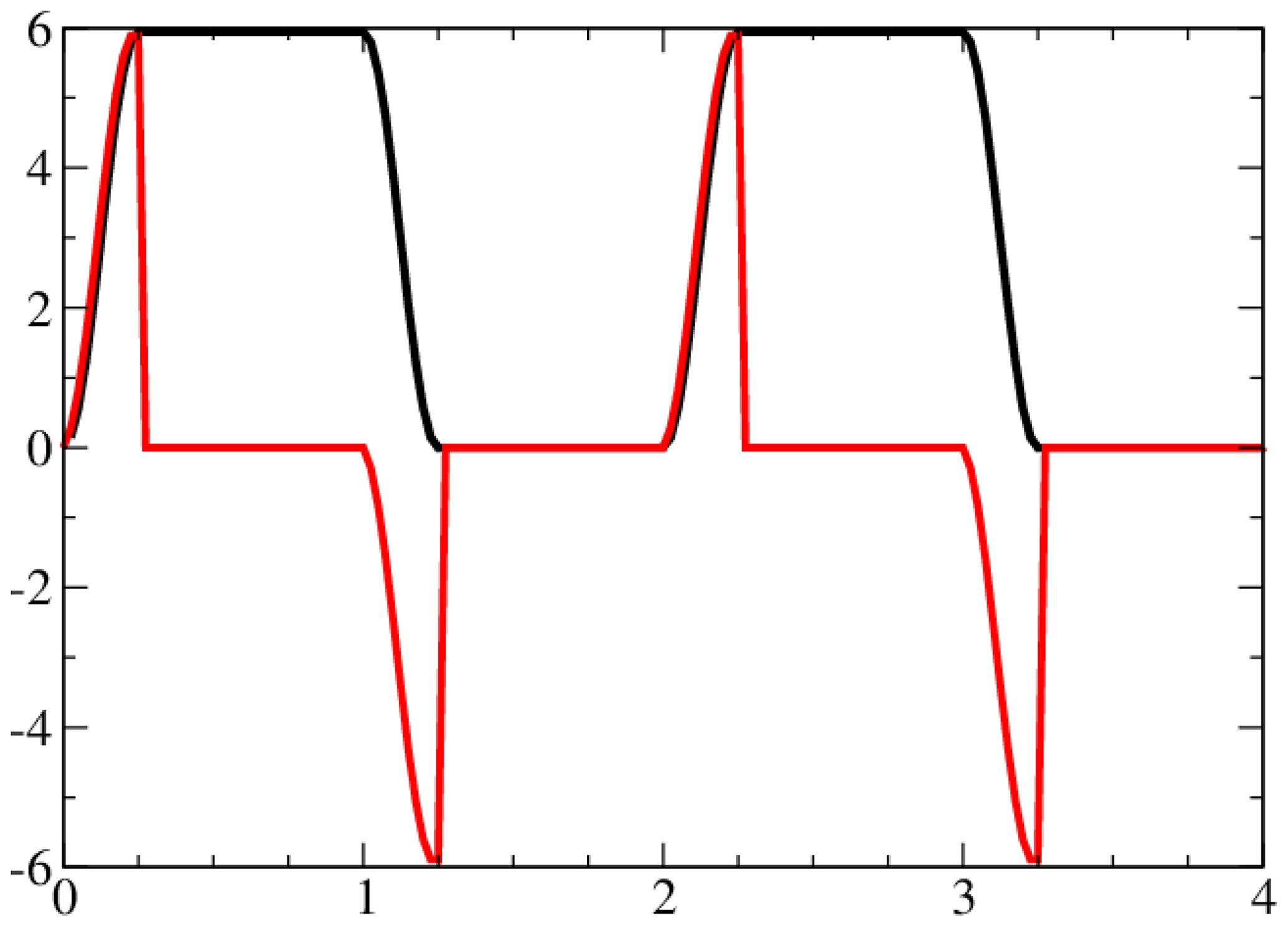
Figure 3 Evolution of the free energy (black) and the work performed on the integrated mode (red) from the numerical integration is shown. The evolution is deterministic and periodic and results agree with the analytic solution.

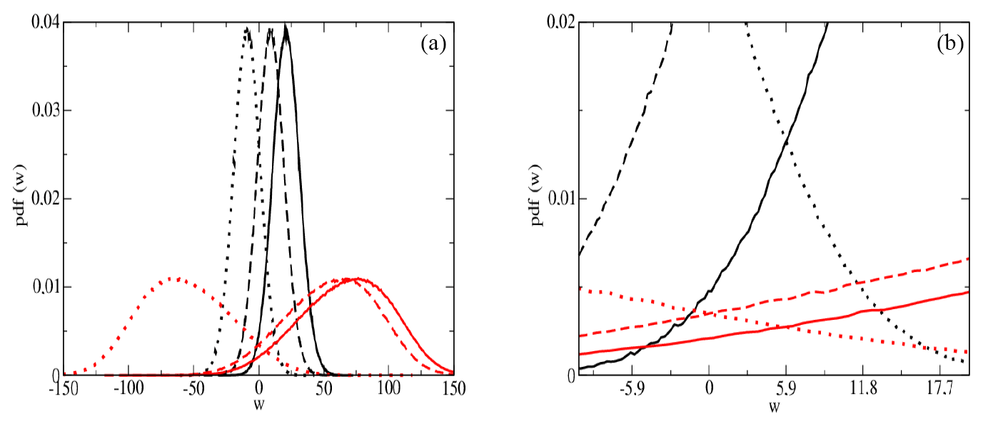
Figure 4 The forward pdf (pdf^f(z), solid line), the backward pdf (pdf^r(z), dashed line), and the negative of the backward pdf (pdf^r(−z), dotted line); exp1 is in black, and exp2 is in red. Solid and dotted lines intersect at Δz=5.9 as can be seen in the enlargement (b). Exp2 is clearly non-Gaussian.

For this model the free energy is still given by the kinetic energy of the integrated mode, as all other motion decays when forcing subsides. It is governed by the same equation as in the linear 0D Coriolis model; that is, its dynamics is independent of the shear and the internal modes in the atmosphere and the ocean. We call $T=\mathrm{4}\mathit{\pi }{f}^{-\mathrm{1}}=\mathrm{1}$ d. The forcing protocol is a constant force that is applied in the intervals $[jT,(j+.25\left)T\right]$ for the days $j=\mathrm{1},\mathrm{\dots },n$. The forcing is applied to the x component only through a large-scale pressure gradient via a geostrophic velocity: ${\mathcal{F}}_x=-(-\mathrm{1}{)}^{j}f{v}_G$ and ℱ_y=0 in Eqs. (1a) and (1b), respectively; that is, the forward and reverse forcing alternate periodically. The periodic work applied to the integrated mode and the evolution of the free energy are shown in Fig. 3; both agree with the analytic solution, and the periodic response to the periodic forcing is clearly visible. This verifies that the dynamics of the integrated mode is not affected by the random fluctuations in the shear coefficient.

The dynamics of the shear mode is governed by the same equations as in the linear 0D Coriolis model with a deterministic forcing and friction at the air–sea interface. The difference to the 0D model is that the dynamics of the internal modes within the atmosphere and the ocean are explicitly resolved and they influence the shear force that acts on the shear mode. That is, the stochastic term in the 0D models mimics the influence of the internal modes in the atmosphere and the ocean. The 1D model also resolves the shear modes, not only between the atmosphere and the ocean but also within them. These modes interact in a non-linear way and exchange energy, which is ultimately dissipated when the external forcing subsides. In the 1D model the internal modes within the atmosphere and within the ocean interact through the surface friction term and the internal eddy viscosities. In more involved 2D or 3D models, not studied here, they also interact through non-linear horizontal advection.

The numerical model to solve the above-discussed equations is a variation on the one used in (Lemarié et al., 2021). There are 20 levels in the atmosphere and 20 in the ocean, with the first grid points at δ_a=5 and δ_o=1 m, in the atmosphere and the ocean, respectively. The time step of the integration is 10π s. For both experiments, the integration consists of a spin-up of 4×10³ d followed by an integration of 4.4×10³ d; the ensemble size is of each integration is 10³, and 10 integrations were performed. The total ensemble size for each experiment is therefore 2.2×10⁷, when we suppose ergodicity (note that the protocol repeats every 2 d).

The work performed on the atmosphere is now a random process. The numerical results show that the average work performed on the atmosphere in the forward process in the two experiments is ΔW^exp.1=21.0 and ΔW^exp.2=67.3 J m⁻², while only a small part of this work drives the integrated mode, contributing to the free energy $\mathrm{\Delta }G=\mathrm{6}/\mathrm{101}\approx \mathrm{5.94}$. Its value can be calculated analytically; it is independent of the friction process and therefore equal in both experiments. Results of the numerical integration are shown in Fig. 4 where the different pdf's are visualized. The standard deviations of the pdf's are σ^exp.1=10.3 and σ^exp.2=34.8 J m⁻². They are close to but significantly different from Gaussian with a skewness (third standardized moment) of ${\mathit{\mu }}_{\mathrm{3}}^{\exp .1}=\mathrm{0.03}$ and ${\mathit{\mu }}_{\mathrm{3}}^{\exp .2}=-\mathrm{0.20}$. In this case the verification of the work theorems no longer reduces to algebraic relations between the first- and second-order moments, but the whole shape of the pdf's has to be considered. The forward pdf and the backward pdf flipped at z=0 (pdf^r(−z)) intersect at ΔG, in both experiments (Fig. 4), within the statistical error as predicted by the CR. The forward pdf and the backward pdf shifted by 2ΔG superpose within statistical error, as can be seen in Fig. 4. This is a consequence of the independence of the deterministic dynamics of the integrated mode from the rest of the dynamics and the symmetry of the forcing protocol given in Eq. (23). The same figure shows clearly that the probability of a forward event with work smaller than the free energy ΔG is non-negligible; the equivalents of such events in thermal processes are referred to as violations of the second law of thermodynamics. Note that the probability of a forward event with negative work is also present.

We numerically found the JE $\langle \exp (-{\mathit{\beta }}_{\mathrm{JE}}(w-\mathrm{\Delta }G){\rangle }_f=\mathrm{1}$ in the two experiments to be satisfied for ${\mathit{\beta }}_{\mathrm{JE}}^{\exp .1}=\mathrm{0.115}$ and ${\mathit{\beta }}_{\mathrm{JE}}^{\exp .2}=\mathrm{0.290}$, respectively, as can be seen from Fig. 5. Here we denote by β_JE the value of β_D obtained from the data through the JE.

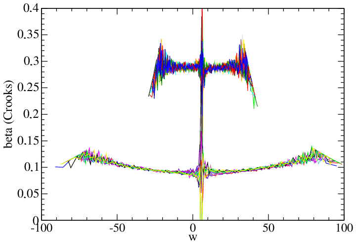
Figure 5 Figure gives β_CR as a function of the work w calculated with the CR Eq. (80), for exp1 (upper graph) and exp2 (lower graph). For each experiment 10 statistically independent realizations are superposed.

For evaluating the CR we plotted

$$\begin{array}{}\text{(80)}& {\mathit{\beta }}_{\mathrm{CR}}={\displaystyle \frac{\mathrm{1}}{w-\mathrm{\Delta }G}}\ln \left({\displaystyle \frac{{\mathrm{pdf}}^f\left(w\right)}{{\mathrm{pdf}}^r(-w)}}\right),\end{array}$$

where we denote by β_CR the value of β_D obtained from the data through the CR. Note that near ΔG this expression is strongly dependent on the bin size, where the nominator and denominator go to zero, which makes a numerical evaluation difficult and leads to strong oscillations. We clearly see that ${\mathit{\beta }}_{\mathrm{CR}}^{\exp .2}$ is close to but significantly different from a constant and that ${\mathit{\beta }}_{\mathrm{JE}}^{\exp .2}$ is a good approximation for values around the maximum of pdf^f(w). The dimension of β is the inverse of an energy, and the obvious question is to see how it can be related to the dynamics. In the Gaussian case Eq. (70) shows that it is equal to the ratio of the heat dissipated over one cycle and the variance of the work:

$$\begin{array}{}\text{(81)}& {\mathit{\beta }}_{\mathrm{Gauss}}={\displaystyle \frac{(W_f+W_r)}{{\mathit{\sigma }}^{\mathrm{2}}}}.\end{array}$$

For the present non-Gaussian model these calculations lead to ${\mathit{\beta }}_{\mathrm{Gauss}}^{\exp .1}=\mathrm{0.29}$ and ${\mathit{\beta }}_{\mathrm{Gauss}}^{\exp .2}=\mathrm{0.10}$; the value is equal to β_CR and β_JE for exp1 (with a close to Gaussian pdf) and close to β_CR and β_JE for exp2 (see from Fig. 5).

4 Discussion

We started by introducing the concept of work theorems into a simple model of air–sea interaction, in which the atmosphere and ocean were represented by their corresponding mixed layer. In this case the JE and the CR can be obtained analytically. We then performed the same calculations on a model including a Coriolis force. In that case the time reversibility is broken and the dynamics lags detailed balance, which is at the basis of the original proofs of the JE and the CR in the Hamiltonian system. Analytical integrations of the stochastic differential equations governing the dynamics of the system prove the existence of the JE and the CR. They furthermore show that the limit of f→0 is well defined and the non-rotating solution is obtained

In the applications of work theorems where fluctuations arise from thermal dynamics, the thermodynamic β is fixed by the temperature of the heat bath. In the system considered here there is no external heat bath, but the fluctuations are generated by the external forcing and the internal dynamics. The different value of the dynamic β in the two experiments comes, therefore, at no surprise, as the fluctuations now arise from the dynamics of the shear mode and the internal modes in the atmosphere and the ocean, which clearly differ between both experiments. In terms of heat fluctuations this means that the system is not thermostated; there is no outside heat bath that keeps the temperature (or β) constant. In exp2 the variation in the drag coefficient is 10 times slower than in exp1 and the dynamics of the shear mode and the internal modes in the atmosphere and the ocean have more time to adjust to its instantaneous value. The drag influences not only the work but also the variability, leading to a dynamic β that depends on w. The result that a variation in the dynamic β is undetectable in exp1 and small in exp2 allows for the definition of an average β in the present dynamics. This shows the pertinence of the work theorems by Jarzynski and Crooks in the present context as they apply not only to exp1 but also to exp2 in which the fluctuations are slower than the forcing protocol. This is important as forcing protocols and turbulence levels vary over a large continuum of timescales.

The physical interpretation of the dynamic β or its inverse, often called effective temperature (Feitosa and Menon, 2004) or characteristic energy (Ciliberto et al., 2004), is given by Eq. (81) as the ratio of the heat dissipated over one cycle to the variance of the work.

5 Conclusions

We have shown that the modern concepts of non-equilibrium statistical mechanics can be applied to large-scale environmental fluid dynamics, where fluctuations are not thermal but come from the turbulent fluid motion. We have demonstrated that the concepts of the dynamic beta, that is the equivalent of temperature in dynamical systems, can be extended to the momentum transfer at the air–sea interface using the formalism developed by Jarzynski and Crooks. It is important to note that work theorems are valid for forces of arbitrary amplitude; they are not a perturbative theory. This is, to the best of our knowledge, the first time that the concepts of work relations are investigated in geophysics and climate science. We successfully adapted the work theorems to the subject of air–sea momentum transfer, but they can, in the same way, be applied to other components of the climate system.

Work theorems also have important practical applications. When the work pdf's of the forward and backward process are obtained, the free energy of the system and the dissipated energy can be obtained and a mechanical efficiency of the air–sea momentum transfer calculated. This is key in understanding the energetics of the climate system. For a discussion of the ocean circulation kinetic energy, we refer the reader to Ferrari and Wunsch (2009), and for a spatio-temporal variability in the momentum transfer to the ocean, we refer to Wirth (2021). When the CR applies, the likeliness of some rare and extreme events can be obtained from parts of the pdf that represent likely events. Furthermore, when work theorems are found to apply in observations, they represent an important tool to evaluate numerical integrations and parameterizations in models of the environmental dynamics.

The mechanics of air–sea momentum transfer has advanced considerably since the pioneering work of Ekman (1905) and is today an active field of research (Duhaut and Straub, 2006; McWilliams and Huckle, 2006; Zhai et al., 2012; Shrira and Almelah, 2020). In an environment fluctuating on a vast continuum of scales in space and time, the statistical mechanics has to be advanced.

The difficulty in performing simulations in air–sea interaction is the large difference in the characteristic timescales of the fast atmosphere and the slow ocean, the stiffness of the problem. Therefore integrations of the fast atmospheric dynamics are necessary with a long spin-up, as the ocean has to be in a statistically stationary state followed by a long integration to obtain a statistical significant ensemble of ocean states. When observations are considered, the stiffness asks for observations over extended periods of time which are just becoming available.

Similar problems appear when the interaction of other components of the climate system are considered. The momentum transfer at the air–sea interface is just one example where work relations between fluctuating components of the climate system increase our understanding. Their extension to other components is straightforward.

Appendix A: The linear 0D1C model

A1 Solution

We consider a state vector given by the atmospheric and oceanic velocity:

$$\begin{array}{}\text{(A1)}& \mathbf{u}\left(t\right)=\left(\begin{array}{c}{u}_{\mathrm{a}}\left(t\right)\\ u_{\mathrm{o}}\left(t\right)\end{array}\right).\end{array}$$

The evolution equation for the 0D1C model (i.e., model of Eq. 9 with f=0) can be written in a matrix form as

$$\begin{array}{}\text{(A2)}& {\partial }_t\mathbf{u}=\mathbf{Pu}+{\mathbf{F}}^{\mathrm{ext}},\end{array}$$

with

$$\begin{array}{}\text{(A3)}& \begin{array}{rl}& \mathbf{P}=-S\left(\begin{array}{ll}m& -m\\ -\mathrm{1}& \mathrm{1}\end{array}\right)\\ & \mathrm{and}{\mathbf{F}}^{\mathrm{ext}}=\mathcal{F}\left(\begin{array}{l}\mathrm{1}\\ \mathrm{0}\end{array}\right)+{\displaystyle \frac{\mathit{\zeta }}{M}}\left(\begin{array}{l}m\\ -\mathrm{1}\end{array}\right),\end{array}\end{array}$$

where ℱ is the deterministic forcing of the synoptic atmosphere on the atmospheric boundary layer and ζ is the random noise parameterizing internal turbulent motion which does not act on the integrated momentum.

The first step to solve the system of ordinary differential equations (ODEs) (Eq. A2) is to diagonalize P. The eigenvalues λ_j and associated eigenvectors e_j of P are

$$\begin{array}{}\text{(A4)}& {\mathit{\lambda }}_{\mathrm{1}}=\mathrm{0},{\mathbf{e}}_{\mathrm{1}}=\left(\begin{array}{c}\mathrm{1}\\ \mathrm{1}\end{array}\right);{\mathit{\lambda }}_{\mathrm{2}}=-\mathrm{SM},{\mathbf{e}}_{\mathrm{2}}=\left(\begin{array}{c}m\\ -\mathrm{1}\end{array}\right),\end{array}$$

with $M=m+\mathrm{1}$. The square matrix P is thus diagonalizable and can be decomposed as

$$\begin{array}{}\text{(A5)}& \mathbf{P}={\mathbf{ADA}}^{-\mathrm{1}},\mathrm{with}\mathbf{A}=\left(\begin{array}{cc}\mathrm{1}& m\\ \mathrm{1}& -\mathrm{1}\end{array}\right),\mathbf{D}=\left(\begin{array}{cc}\mathrm{0}& \mathrm{0}\\ \mathrm{0}& -\mathrm{SM}\end{array}\right).\end{array}$$

Furthermore, $M{\mathbf{A}}^{-\mathrm{1}}=\mathbf{A}$ and also

$${\mathbf{A}}^{-\mathrm{1}}\mathbf{u}={\displaystyle \frac{\mathrm{1}}{M}}\left(\mathbf{Au}\right)={\displaystyle \frac{\mathrm{1}}{M}}\left(\begin{array}{c}{u}_{\mathrm{a}}+m{u}_{\mathrm{o}}\\ u_{\mathrm{a}}-u_{\mathrm{o}}\end{array}\right)={\displaystyle \frac{\mathrm{1}}{M}}\left(\begin{array}{c}{u}_I\\ u_S\end{array}\right),$$

which shows that the integrated u_I and shear u_S modes defined in Eq. (10) are eigenmodes of the dynamics. We can thus re-express Eq. (A2) with the unknown u as

$$\begin{array}{}\text{(A6)}& {\partial }_t{\mathbf{u}}_M={\mathbf{Du}}_M+{\mathbf{AF}}^{\mathrm{ext}},{\mathbf{u}}_M=\left(\begin{array}{c}{u}_I\\ u_S\end{array}\right),\end{array}$$

with the unknown u_M. Because D is a diagonal matrix, the two ODEs in Eq. (A6) are decoupled and can be solved separately. As reported in Eq. (39), we easily find that

$$\begin{array}{}\text{(A7)}& \begin{array}{rl}{\mathbf{u}}_M\left(t\right)& =\left(\begin{array}{cc}\mathrm{1}& \mathrm{0}\\ \mathrm{0}& e^{-MSt}\end{array}\right){\mathbf{u}}_M\left(\mathrm{0}\right)\\ & +\underset{\mathrm{0}}{\overset{t}{\int }}\left(\begin{array}{c}\mathcal{F}\left(t^{\prime }\right)\\ e^{-MS(t-t^{\prime })}\left[\mathcal{F}\left(t^{\prime }\right)+\mathit{\zeta }\left(t^{\prime }\right)\right]\end{array}\right)\mathrm{d}{t}^{\prime },\end{array}\end{array}$$

and the solution in terms of the original unknowns u_a and u_o given in Eq. (38) is simply obtained using the relation $\mathbf{u}=\left({\mathbf{Au}}_M\right)/M$ to obtain

$$\begin{array}{}\text{(A8)}& \begin{array}{rl}& \mathbf{u}\left(t\right)={\displaystyle \frac{\mathrm{1}}{M}}\left\{\left(\begin{array}{ll}\mathrm{1}+m{e}^{-MSt}& m(\mathrm{1}-e^{-MSt})\\ \mathrm{1}-e^{-MSt}& m+e^{-MSt}\end{array}\right)\right.\\ & \left.\mathbf{u}\left(\mathrm{0}\right)+\underset{\mathrm{0}}{\overset{t}{\int }}\left(\begin{array}{l}\mathcal{F}\left(t^{\prime }\right)+m{e}^{-MS(t-t^{\prime })}\left[\mathcal{F}\left(t^{\prime }\right)+\mathit{\zeta }\left(t^{\prime }\right)\right]\\ \mathcal{F}\left(t^{\prime }\right)-e^{-MS(t-t^{\prime })}\left[\mathcal{F}\left(t^{\prime }\right)+\mathit{\zeta }\left(t^{\prime }\right)\right]\end{array}\right)\mathrm{d}{t}^{\prime }\right\},\end{array}\end{array}$$

which can be recast as

$$\begin{array}{}\text{(A9a)}& {\displaystyle }\begin{array}{rl}& u_{\mathrm{a}}\left(t\right)=u_{\mathrm{a}}\left(\mathrm{0}\right)-\left(u_{\mathrm{a}}\right(\mathrm{0})-u_{\mathrm{o}}(\mathrm{0}\left)\right){\displaystyle \frac{m}{M}}\left(\mathrm{1}-e^{-MSt}\right)\\ & +\underset{\mathrm{0}}{\overset{t}{\int }}{\displaystyle \frac{\mathrm{1}}{M}}\left(\mathrm{1}+m{e}^{-MS(t-t^{\prime })}\right)\mathcal{F}\left(t^{\prime }\right)\mathrm{d}{t}^{\prime }\\ & +{\displaystyle \frac{m}{M}}\underset{\mathrm{0}}{\overset{t}{\int }}{e}^{-MS(t-t^{\prime })}\mathit{\zeta }\left(t^{\prime }\right)\mathrm{d}{t}^{\prime },\end{array}\text{(A9b)}& {\displaystyle }\begin{array}{rl}{u}_{\mathrm{o}}\left(t\right)& =u_{\mathrm{o}}\left(\mathrm{0}\right)+\left(u_{\mathrm{a}}\right(\mathrm{0})-u_{\mathrm{o}}(\mathrm{0}\left)\right){\displaystyle \frac{\mathrm{1}}{M}}\left(\mathrm{1}-e^{-MSt}\right)\\ & +\underset{\mathrm{0}}{\overset{t}{\int }}{\displaystyle \frac{\mathrm{1}}{M}}\left(\mathrm{1}-e^{-MS(t-t^{\prime })}\right)\mathcal{F}\left(t^{\prime }\right)\mathrm{d}{t}^{\prime }\\ & -{\displaystyle \frac{\mathrm{1}}{M}}\underset{\mathrm{0}}{\overset{t}{\int }}{e}^{-MS(t-t^{\prime })}\mathit{\zeta }\left(t^{\prime }\right)\mathrm{d}{t}^{\prime }.\end{array}\end{array}$$

A2 Variance

The deterministic and the stochastic dynamics are statistically independent, so when calculating statistical moments we can ignore the deterministic one (i.e., ℱ(t) will be ignored). In the following we denote $u_S^{\prime }$ as the random part of u_S. The solution of the shear mode is given by Eq. (39b). Its variance is, using the fact that $〈\mathit{\zeta }\left(t\right)\mathit{\zeta }\left(t^{\prime }\right)〉=\mathrm{2}R\mathit{\delta }(t-t^{\prime })$ (see Eq. 40) and that 〈ζ(t)〉=0,

$$\begin{array}{}\text{(A10)}& \begin{array}{rl}\langle u_S^{\prime }(t{)}^{\mathrm{2}}\rangle & =〈{\left(\underset{\mathrm{0}}{\overset{t}{\int }}{e}^{-\mathrm{SM}(t-t^{\prime })}\mathit{\zeta }\left(t^{\prime }\right)\mathrm{d}{t}^{\prime }+u_S\left(\mathrm{0}\right)e^{-\mathrm{SM}t}\right)}^{\mathrm{2}}〉\\ & =\underset{\mathrm{0}}{\overset{t}{\int }}\underset{\mathrm{0}}{\overset{t}{\int }}{e}^{-\mathrm{SM}(t-t^{\prime })}{e}^{-\mathrm{SM}(t-t^{\prime \prime })}\langle \mathit{\zeta }\left(t^{\prime \prime }\right)\mathit{\zeta }\left(t^{\prime }\right)\rangle \mathrm{d}{t}^{\prime \prime }\mathrm{d}{t}^{\prime }\\ & +e^{-\mathrm{2}\mathrm{SM}t}\langle u_S^{\prime }(\mathrm{0}{)}^{\mathrm{2}}\rangle \\ & =\mathrm{2}R\underset{\mathrm{0}}{\overset{t}{\int }}{e}^{-\mathrm{SM}(t-\mathrm{2}{t}^{\prime })}\mathrm{d}{t}^{\prime }+e^{-\mathrm{2}\mathrm{SM}t}\langle u_S(\mathrm{0}{)}^{\mathrm{2}}\rangle \\ & ={\displaystyle \frac{R}{\mathrm{SM}}}(\mathrm{1}-e^{-\mathrm{2}\mathrm{SM}t})+e^{-\mathrm{2}\mathrm{SM}t}\langle u_S^{\prime }(\mathrm{0}{)}^{\mathrm{2}}\rangle .\end{array}\end{array}$$

It is important to note that there are two different averages involved in the above equation, all denoted by the same symbol 〈⋅〉. One is over the noise, and the other is over the initial conditions. Using the same symbol is justified as the initial conditions are due to the same statistical noise applied prior to t=0. In a statistically stationary process the variance is independent of the time t, and therefore

$$\begin{array}{}\text{(A11)}& \langle u_S^{\prime }(t{)}^{\mathrm{2}}\rangle =\langle u_S^{\prime }(\mathrm{0}{)}^{\mathrm{2}}\rangle ={\displaystyle \frac{R}{\mathrm{SM}}}.\end{array}$$

Such a consistency condition is extensively used throughout this paper.

For the work theorems the focus is on the statistics of averages over a time interval T. Using Eq. (A7) we obtain

$$\begin{array}{}\text{(A12)}& \begin{array}{rl}{\stackrel{\mathrm{‾}}{u_S^{\prime }}}^T\left(t\right)& ={\displaystyle \frac{\mathrm{1}}{T}}\underset{\mathrm{0}}{\overset{T}{\int }}{u}_S^{\prime }(t+T^{\prime })\mathrm{d}{T}^{\prime }={\displaystyle \frac{\mathrm{1}}{T}}\underset{\mathrm{0}}{\overset{T}{\int }}\underset{\mathrm{0}}{\overset{t+T^{\prime }}{\int }}{e}^{-\mathrm{SM}(t+T^{\prime }-t^{\prime })}\\ & \mathit{\zeta }\left(t^{\prime }\right)\mathrm{d}{t}^{\prime }+u_S\left(\mathrm{0}\right)e^{-\mathrm{SM}(t+T^{\prime })}\mathrm{d}{T}^{\prime }\\ & ={\displaystyle \frac{e^{-\mathrm{SM}t}}{T}}\underset{\mathrm{0}}{\overset{T}{\int }}\underset{\mathrm{0}}{\overset{t+T^{\prime }}{\int }}{e}^{-\mathrm{SM}(T^{\prime }-t^{\prime })}\mathit{\zeta }\left(t^{\prime }\right)\mathrm{d}{t}^{\prime }\mathrm{d}{T}^{\prime }\\ & +{\displaystyle \frac{e^{-\mathrm{SM}t}}{\mathrm{SM}T}}(\mathrm{1}-e^{-\mathrm{SM}T})u_S\left(\mathrm{0}\right).\end{array}\end{array}$$

Its variance is

$$\begin{array}{}\text{(A13)}& \begin{array}{rl}\langle [{\stackrel{\mathrm{‾}}{u_S^{\prime }}}^T& \left(t\right){]}^{\mathrm{2}}\rangle ={\displaystyle \frac{e^{-\mathrm{2}\mathrm{SM}t}}{T^{\mathrm{2}}}}\underset{\mathrm{0}}{\overset{T}{\int }}\underset{\mathrm{0}}{\overset{T}{\int }}\underset{\mathrm{0}}{\overset{t+T^{\prime }}{\int }}\underset{\mathrm{0}}{\overset{t+T^{\prime \prime }}{\int }}{e}^{-\mathrm{SM}(T^{\prime }-t^{\prime }+T^{\prime \prime }-t^{\prime \prime })}\\ & \langle \mathit{\zeta }\left(t^{\prime }\right)\mathit{\zeta }\left(t^{\prime \prime }\right)\rangle \mathrm{d}{t}^{\prime \prime }\mathrm{d}{t}^{\prime }\mathrm{d}{T}^{\prime \prime }\mathrm{d}{T}^{\prime }+{\displaystyle \frac{e^{-\mathrm{2}\mathrm{SM}t}}{(\mathrm{SM}T{)}^{\mathrm{2}}}}\\ & (\mathrm{1}-e^{-\mathrm{SM}T}{)}^{\mathrm{2}}\langle u_S(\mathrm{0}{)}^{\mathrm{2}}\rangle \\ & [\mathrm{define}:\stackrel{\mathrm{̃}}{T}=min(T^{\prime },T^{\prime \prime }\left)\right]\\ & ={\displaystyle \frac{\mathrm{2}R{e}^{-\mathrm{2}\mathrm{SM}t}}{T^{\mathrm{2}}}}\underset{\mathrm{0}}{\overset{T}{\int }}\underset{\mathrm{0}}{\overset{T}{\int }}\underset{\mathrm{0}}{\overset{t+\stackrel{\mathrm{̃}}{T}}{\int }}{e}^{-\mathrm{SM}(T^{\prime }+T^{\prime \prime }-\mathrm{2}{t}^{\prime })}\\ & \mathrm{d}{t}^{\prime }\mathrm{d}{T}^{\prime \prime }\mathrm{d}{T}^{\prime }+{\displaystyle \frac{e^{-\mathrm{2}\mathrm{SM}t}}{(\mathrm{SM}T{)}^{\mathrm{2}}}}(\mathrm{1}-e^{-\mathrm{SM}T}{)}^{\mathrm{2}}{\displaystyle \frac{R}{\mathrm{SM}}}\\ & ={\displaystyle \frac{R}{\mathrm{SM}{T}^{\mathrm{2}}}}\underset{\mathrm{0}}{\overset{T}{\int }}\underset{\mathrm{0}}{\overset{T}{\int }}{e}^{-\mathrm{SM}(T^{\prime }+T^{\prime \prime }-\mathrm{2}\stackrel{\mathrm{̃}}{T})}\\ & -e^{-\mathrm{SM}(T^{\prime }+T^{\prime \prime }+\mathrm{2}t)}\mathrm{d}{T}^{\prime \prime }\mathrm{d}{T}^{\prime }+{\displaystyle \frac{e^{-\mathrm{2}\mathrm{SM}t}}{(\mathrm{SM}T{)}^{\mathrm{2}}}}\\ & (\mathrm{1}-e^{-\mathrm{SM}T}{)}^{\mathrm{2}}{\displaystyle \frac{R}{\mathrm{SM}}}\\ & ={\displaystyle \frac{\mathrm{2}R}{\mathrm{SM}{T}^{\mathrm{2}}}}\underset{\mathrm{0}}{\overset{T}{\int }}\underset{\mathrm{0}}{\overset{T^{\prime }}{\int }}{e}^{-\mathrm{SM}(T^{\prime }-T^{\prime \prime })}-e^{-\mathrm{SM}(T^{\prime }+T^{\prime \prime }+\mathrm{2}t)}\\ & \mathrm{d}{T}^{\prime \prime }\mathrm{d}{T}^{\prime }+{\displaystyle \frac{e^{-\mathrm{2}\mathrm{SM}t}}{(\mathrm{SM}T{)}^{\mathrm{2}}}}(\mathrm{1}-e^{-\mathrm{SM}T}{)}^{\mathrm{2}}{\displaystyle \frac{R}{\mathrm{SM}}}\\ & ={\displaystyle \frac{\mathrm{2}R}{(\mathrm{SM}T{)}^{\mathrm{2}}}}\underset{\mathrm{0}}{\overset{T}{\int }}\mathrm{1}-e^{-\mathrm{SM}{T}^{\prime }}+e^{-\mathrm{SM}(\mathrm{2}{T}^{\prime }+\mathrm{2}t)}\\ & -e^{-\mathrm{SM}(T^{\prime }+\mathrm{2}t)}\mathrm{d}{T}^{\prime }+{\displaystyle \frac{e^{-\mathrm{2}\mathrm{SM}t}}{(\mathrm{SM}T{)}^{\mathrm{2}}}}(\mathrm{1}-e^{-\mathrm{SM}T}{)}^{\mathrm{2}}\\ & {\displaystyle \frac{R}{\mathrm{SM}}}={\displaystyle \frac{\mathrm{2}R}{(\mathrm{SM}T{)}^{\mathrm{2}}}}[T+{\displaystyle \frac{e^{-\mathrm{SM}T}-\mathrm{1}}{\mathrm{SM}}}\\ & -e^{-\mathrm{2}\mathrm{SM}t}\left({\displaystyle \frac{e^{-\mathrm{2}\mathrm{SM}T}-\mathrm{1}-\mathrm{2}{e}^{-\mathrm{SM}T}+\mathrm{2}}{\mathrm{2}\mathrm{SM}}}\right)]\\ & +{\displaystyle \frac{e^{-\mathrm{2}\mathrm{SM}t}}{(\mathrm{SM}T{)}^{\mathrm{2}}}}(\mathrm{1}-e^{-\mathrm{SM}T}{)}^{\mathrm{2}}{\displaystyle \frac{R}{\mathrm{SM}}}\\ & ={\displaystyle \frac{\mathrm{2}R}{(\mathrm{SM}{)}^{\mathrm{3}}{T}^{\mathrm{2}}}}[\mathrm{SM}T+e^{-\mathrm{SM}T}-\mathrm{1}]\\ & ={\displaystyle \frac{\mathrm{2}R}{Sm({\mathcal{F}}_{\mathrm{0}}T{)}^{\mathrm{2}}}}{W}_S.\end{array}\end{array}$$

Note that for T≪SM we have $\langle \left[{\stackrel{\mathrm{‾}}{u_S^{\prime }}}^T\right(t){]}^{\mathrm{2}}\rangle =\langle u_S(t{)}^{\mathrm{2}}\rangle$, and for T≫SM we obtain $\langle \left[{\stackrel{\mathrm{‾}}{u_S^{\prime }}}^T\right(t){]}^{\mathrm{2}}\rangle =\mathrm{2}\langle u_S(t{)}^{\mathrm{2}}\rangle /\left(\mathrm{SM}T\right)$.

Appendix B: The linear 0D2C model

The calculations performed for the one-component model in the previous section will now be extended to the two-component model where the two components interact through the Coriolis force.

B1 Solution

To simplify the algebra we temporarily manipulate complex quantities in this subsection. For the 0D2C model given in Eq. (9) we consider a state vector given by

$$\begin{array}{}\text{(B1)}& \mathbf{y}\left(t\right)=\left(\begin{array}{c}{U}_{\mathrm{a}}\left(t\right)\\ U_{\mathrm{o}}\left(t\right)\end{array}\right),\end{array}$$

where U_a and U_o are complex quantities such that $U_{\mathrm{a}}=u_{\mathrm{a}}+i{v}_{\mathrm{a}}$ and $U_{\mathrm{o}}=u_{\mathrm{o}}+i{v}_{\mathrm{o}}$. The general evolution equation satisfied by y is

$$\begin{array}{}\text{(B2)}& {\partial }_t\mathbf{y}={\mathbf{P}}_f\mathbf{y}+{\mathbf{F}}_f^{\mathrm{ext}},\end{array}$$

with

$$\begin{array}{}\text{(B3)}& \begin{array}{rl}& {\mathbf{P}}_f=\begin{array}{ll}-\mathrm{if}-Sm& Sm\\ S& -\mathrm{if}-S\end{array}\\ & \mathrm{and}{\mathbf{F}}_f^{\mathrm{ext}}=\begin{array}{c}\mathcal{F}\\ \mathrm{0}\end{array}+{\displaystyle \frac{\mathrm{1}}{M}}({\mathit{\zeta }}_x+i{\mathit{\zeta }}_y)\begin{array}{c}m\\ -\mathrm{1}\end{array},\end{array}\end{array}$$

where F_u, ζ_u and ζ_v are real-valued functions. The matrix P_f is diagonalizable and can be decomposed as

$$\begin{array}{}\text{(B4)}& \begin{array}{rl}{\mathbf{P}}_f& ={\mathbf{AD}}_f{\mathbf{A}}^{-\mathrm{1}},\mathrm{with}\mathbf{A}=\left(\begin{array}{ll}\mathrm{1}& m\\ \mathrm{1}& -\mathrm{1}\end{array}\right),\\ & {\mathbf{D}}_f=\left(\begin{array}{ll}-\mathrm{if}& \mathrm{0}\\ \mathrm{0}& -\mathrm{if}-\mathrm{SM}\end{array}\right).\end{array}\end{array}$$

We recall that $M{\mathbf{A}}^{-\mathrm{1}}=\mathbf{A}$, and introducing the complex numbers $U_I=u_I+i{v}_I$ and $U_S=u_S+i{v}_S$ corresponding to the integrated and shear modes, we have

$${\mathbf{A}}^{-\mathrm{1}}\mathbf{y}={\displaystyle \frac{\mathrm{1}}{M}}\left(\mathbf{Ay}\right)={\displaystyle \frac{\mathrm{1}}{M}}{\mathbf{y}}_M,{\mathbf{y}}_M=\left(\begin{array}{c}{U}_I\\ U_S\end{array}\right).$$

Re-expressing the original system of ODEs in terms of y_M, we obtain

$${\partial }_t{\mathbf{y}}_M={\mathbf{D}}_f{\mathbf{y}}_M+{\mathbf{AF}}_f^{\mathrm{ext}},$$

and we obtain two independent ODEs for the complex functions U_I(t) and U_S(t):

$$\begin{array}{}\text{(B5a)}& {\displaystyle }{\partial }_t{U}_I=-if{U}_I+\mathcal{F}\left(t\right),\text{(B5b)}& {\displaystyle }{\partial }_t{U}_S=(-if-SM)U_S+\mathcal{F}\left(t\right)+\left({\mathit{\zeta }}_x\right(t)+i{\mathit{\zeta }}_y(t\left)\right),\end{array}$$

whose solutions are

$$\begin{array}{}\text{(B6a)}& {\displaystyle }\begin{array}{rl}{U}_I\left(t\right)& =U_I\left(\mathrm{0}\right)e^{-ift}\\ & +\underset{\mathrm{0}}{\overset{t}{\int }}{e}^{-if(t-t^{\prime })}\mathcal{F}\left(t^{\prime }\right)\mathrm{d}{t}^{\prime },\end{array}\text{(B6b)}& {\displaystyle }\begin{array}{rl}{U}_S\left(t\right)& =U_S\left(\mathrm{0}\right)e^{-(if+\mathrm{SM})t}+\underset{\mathrm{0}}{\overset{t}{\int }}{e}^{-(if+SM)(t-t^{\prime })}\\ & \left[\mathcal{F}\left(t^{\prime }\right)+\left({\mathit{\zeta }}_x\right(t^{\prime })+i{\mathit{\zeta }}_y(t^{\prime }\left)\right)\right]\mathrm{d}{t}^{\prime }.\end{array}\end{array}$$

Taking the real and imaginary parts of U_I(t), we obtain

$$\begin{array}{}\text{(B7a)}& {\displaystyle }\begin{array}{rl}{u}_I\left(t\right)& =\cos \left(ft\right)u_I\left(\mathrm{0}\right)+\sin \left(ft\right)v_I\left(\mathrm{0}\right)\\ & +\underset{\mathrm{0}}{\overset{t}{\int }}\cos \left(f\right(t-t^{\prime }\left)\right)\mathcal{F}\left(t^{\prime }\right)\mathrm{d}{t}^{\prime },\end{array}\text{(B7b)}& {\displaystyle }\begin{array}{rl}{v}_I\left(t\right)& =\cos \left(ft\right)v_I\left(\mathrm{0}\right)-\sin \left(ft\right)u_I\left(\mathrm{0}\right)\\ & +\underset{\mathrm{0}}{\overset{t}{\int }}\sin \left(f\right(t-t^{\prime }\left)\right)\mathcal{F}\left(t^{\prime }\right)\mathrm{d}{t}^{\prime }.\end{array}\end{array}$$

Now considering the shear mode, we have

$$\begin{array}{ll}{\displaystyle }{u}_S\left(t\right)& {\displaystyle }=e^{-\mathrm{SM}t}\left(\cos \right(ft\left)u_S\right(\mathrm{0})+\sin (ft\left)v_S\right(\mathrm{0}\left)\right)\\ {\displaystyle }& {\displaystyle }+\underset{\mathrm{0}}{\overset{t}{\int }}{e}^{-\mathrm{SM}(t-t^{\prime })}\left[\right(\mathcal{F}\left(t^{\prime }\right)+{\mathit{\zeta }}_x\left(t^{\prime }\right)\left)\cos \right(f(t-t^{\prime }))\\ {\displaystyle }& {\displaystyle }+{\mathit{\zeta }}_y\left(t^{\prime }\right)\sin \left(f\right(t-t^{\prime }\left)\right)]\mathrm{d}{t}^{\prime }\\ {\displaystyle }& {\displaystyle }{v}_S\left(t\right)=e^{-\mathrm{SM}t}\left(\cos \right(ft\left)v_S\right(\mathrm{0})-\sin (ft\left)u_S\right(\mathrm{0}\left)\right)\\ {\displaystyle }& {\displaystyle }+\underset{\mathrm{0}}{\overset{t}{\int }}{e}^{-\mathrm{SM}(t-t^{\prime })}\left[{\mathit{\zeta }}_y\right(t^{\prime }\left)\cos \right(f(t-t^{\prime }))-(\mathcal{F}\left(t^{\prime }\right)\\ {\displaystyle }& {\displaystyle }+{\mathit{\zeta }}_x\left(t^{\prime }\right)\left)\sin \right(f(t-t^{\prime })\left)\right]\mathrm{d}{t}^{\prime }.\end{array}$$

Note that for f=0, we easily recover the solutions from the 0D1C model. To further simplify those solutions, we introduce the notations

$$\begin{array}{}\text{(B9)}& \begin{array}{rl}& {\mathcal{C}}_I\left(x\right)=\underset{\mathrm{0}}{\overset{t}{\int }}\cos \left(f\right(t-t^{\prime }\left)\right)x\left(t^{\prime }\right)\mathrm{d}{t}^{\prime }\\ & {\mathcal{C}}_S\left(x\right)=\underset{\mathrm{0}}{\overset{t}{\int }}{e}^{-\mathrm{SM}(t-t^{\prime })}\cos \left(f\right(t-t^{\prime }\left)\right)x\left(t^{\prime }\right)\mathrm{d}{t}^{\prime }\\ & {\mathcal{S}}_I\left(x\right)=\underset{\mathrm{0}}{\overset{t}{\int }}\sin \left(f\right(t-t^{\prime }\left)\right)x\left(t^{\prime }\right)\mathrm{d}{t}^{\prime }\\ & {\mathcal{S}}_S\left(x\right)=\underset{\mathrm{0}}{\overset{t}{\int }}{e}^{-\mathrm{SM}(t-t^{\prime })}\sin \left(f\right(t-t^{\prime }\left)\right)x\left(t^{\prime }\right)\mathrm{d}{t}^{\prime },\end{array}\end{array}$$

to reformulate the solutions of the 0D2C model as

$$\begin{array}{}\text{(B10a)}& {\displaystyle }{\mathbf{u}}_I\left(t\right)=\left(\begin{array}{cc}\cos \left(ft\right)& \sin \left(ft\right)\\ -\sin \left(ft\right)& \cos \left(ft\right)\end{array}\right){\mathbf{u}}_I\left(\mathrm{0}\right)+\left(\begin{array}{c}{\mathcal{C}}_I\left(\mathcal{F}\right)\\ {\mathcal{S}}_I\left(\mathcal{F}\right)\end{array}\right),\text{(B10b)}& {\displaystyle }\begin{array}{rl}{\mathbf{u}}_S\left(t\right)& =\left(\begin{array}{cc}\cos \left(ft\right)& \sin \left(ft\right)\\ -\sin \left(ft\right)& \cos \left(ft\right)\end{array}\right)e^{-\mathrm{SM}t}{\mathbf{u}}_S\left(\mathrm{0}\right)\\ & +\left(\begin{array}{c}{\mathcal{C}}_S\left(\mathcal{F}\right)+{\mathcal{C}}_S\left({\mathit{\zeta }}_x\right)+{\mathcal{S}}_S\left({\mathit{\zeta }}_y\right)\\ {\mathcal{C}}_S\left({\mathit{\zeta }}_y\right)-{\mathcal{S}}_S\left(\mathcal{F}\right)-{\mathcal{S}}_S\left({\mathit{\zeta }}_x\right)\end{array}\right).\end{array}\end{array}$$

B2 Variance

For the sake of clarity we use the notations c=cos (ft) and s=sin (ft) in the following. We consider a Gaussian process with a variance:

$$\begin{array}{}\text{(B11)}& \begin{array}{rl}\langle \left[u_S^{\prime }\right(t){]}^{\mathrm{2}}\rangle & =\mathrm{2}R\underset{\mathrm{0}}{\overset{t}{\int }}{e}^{-\mathrm{2}\mathrm{SM}(t-t^{\prime })}\mathrm{d}{t}^{\prime }+e^{-\mathrm{2}\mathrm{SM}t}(c^{\mathrm{2}}\langle u_S(\mathrm{0}{)}^{\mathrm{2}}\rangle \\ & +s^{\mathrm{2}}\langle v_S(\mathrm{0}{)}^{\mathrm{2}}\rangle +\mathrm{2}cs\langle u_S(\mathrm{0}\left)v_S\right(\mathrm{0})\rangle )\\ & ={\displaystyle \frac{R}{\mathrm{SM}}}(\mathrm{1}-e^{-\mathrm{2}\mathrm{SM}t})+e^{-\mathrm{2}\mathrm{SM}t}\langle u_S(\mathrm{0}{)}^{\mathrm{2}}\rangle \\ & ={\displaystyle \frac{R}{\mathrm{SM}}}.\end{array}\end{array}$$

If the noise is turned off at t=0, we have the deterministic evolution (using $\cos (t+\mathit{\alpha })\cos (t+\mathit{\beta })+\sin (t+\mathit{\alpha })\sin (t+\mathit{\beta })=\cos \mathit{\alpha }\cos \mathit{\beta }+\sin \mathit{\alpha }\sin \mathit{\beta }$)

$$\begin{array}{}\text{(B12)}& \begin{array}{rl}{\stackrel{\mathrm{‾}}{u_S^{\mathrm{0}}}}^T\left(t\right)& ={\displaystyle \frac{e^{-\mathrm{SM}t}}{T}}\underset{\mathrm{0}}{\overset{T}{\int }}{e}^{-\mathrm{SM}{T}^{\prime }}\left(\cos f\right(t+T^{\prime }\left)u_S\right(\mathrm{0})\\ & +\sin f(t+T^{\prime })v_S\left(\mathrm{0}\right))\mathrm{d}{T}^{\prime },\end{array}\end{array}$$

and its variance is given by

$$\begin{array}{}\text{(B13)}& \begin{array}{rl}\langle & \left[{\stackrel{\mathrm{‾}}{u_S^{\mathrm{0}}}}^T\right(t){]}^{\mathrm{2}}\rangle ={\displaystyle \frac{e^{-\mathrm{2}\mathrm{SM}t}}{T^{\mathrm{2}}}}\underset{\mathrm{0}}{\overset{T}{\int }}\underset{\mathrm{0}}{\overset{T}{\int }}{e}^{-\mathrm{SM}(T^{\prime }+T^{\prime \prime })}\\ & \langle \left[\cos f\right(t+T^{\prime })\\ & u_S\left(\mathrm{0}\right)+\sin f(t+T^{\prime })v_S\left(\mathrm{0}\right)]\\ & \left[\cos f\right(t+T^{\prime \prime }\left)u_S\right(\mathrm{0})+\sin f(t+T^{\prime \prime })\\ & v_S\left(\mathrm{0}\right)]\rangle \mathrm{d}{T}^{\prime \prime }\mathrm{d}{T}^{\prime }\\ & ={\displaystyle \frac{R{e}^{-\mathrm{2}\mathrm{SM}t}}{\mathrm{SM}{T}^{\mathrm{2}}}}\underset{\mathrm{0}}{\overset{T}{\int }}\underset{\mathrm{0}}{\overset{T}{\int }}{e}^{-\mathrm{SM}(T^{\prime }+T^{\prime \prime })}(\cos f{T}^{\prime }\\ & \cos f{T}^{\prime \prime }+\sin f{T}^{\prime }\sin f{T}^{\prime \prime })\mathrm{d}{T}^{\prime \prime }\mathrm{d}{T}^{\prime }\\ & ={\displaystyle \frac{R{e}^{-\mathrm{2}\mathrm{SM}t}}{\mathrm{SM}{T}^{\mathrm{2}}}}\left[\right(\underset{\mathrm{0}}{\overset{T}{\int }}{e}^{-\mathrm{SM}{T}^{\prime }}\cos f{T}^{\prime }\mathrm{d}{T}^{\prime }{)}^{\mathrm{2}}\\ & +\left(\underset{\mathrm{0}}{\overset{T}{\int }}{e}^{-\mathrm{SM}{T}^{\prime }}\sin f{T}^{\prime }\mathrm{d}{T}^{\prime }{)}^{\mathrm{2}}\right]\\ & ={\displaystyle \frac{R{e}^{-\mathrm{2}\mathrm{SM}t}(e^{-\mathrm{2}\mathrm{SM}T}-\mathrm{2}{e}^{-\mathrm{2}\mathrm{SM}T}\cos (fT)+\mathrm{1})}{\mathrm{SM}{T}^{\mathrm{2}}\left(\right(\mathrm{SM}{)}^{\mathrm{2}}+f^{\mathrm{2}})}}.\end{array}\end{array}$$

It cancels the time-dependent part of the variance due to the noise (see Eq. B14), making the total variance time independent. This is another expression of the consistency condition mentioned in the previous section. The total variance is

$$\begin{array}{}\text{(B14)}& \begin{array}{rl}\langle \left[{\stackrel{\mathrm{‾}}{u_S^{\prime }}}^T\right(t){]}^{\mathrm{2}}\rangle & =\langle {\left[{\stackrel{\mathrm{‾}}{{\mathcal{C}}_S\left({\mathit{\zeta }}_u\right)+{\mathcal{S}}_S\left({\mathit{\zeta }}_v\right)}}^T+{\stackrel{\mathrm{‾}}{u_S^{\mathrm{0}}}}^T\left(t\right)\right]}^{\mathrm{2}}\rangle \\ & ={\displaystyle \frac{e^{-\mathrm{2}\mathrm{SM}t}}{T^{\mathrm{2}}}}\underset{\mathrm{0}}{\overset{T}{\int }}\underset{\mathrm{0}}{\overset{T}{\int }}{e}^{-\mathrm{SM}(T^{\prime }+T^{\prime \prime })}\underset{\mathrm{0}}{\overset{t+T^{\prime }}{\int }}\underset{\mathrm{0}}{\overset{t+T^{\prime \prime }}{\int }}{e}^{\mathrm{SM}(t^{\prime }+t^{\prime \prime })}\\ & \langle \left[{\mathit{\zeta }}_u\right(t^{\prime }\left)\cos \right(f(t+T^{\prime }-t^{\prime }))+{\mathit{\zeta }}_v(t^{\prime })\\ & \sin \left(f\right(t+T^{\prime }-t^{\prime }\left)\right)\left]\right[{\mathit{\zeta }}_u\left(t^{\prime \prime }\right)\cos \left(f\right(t+T^{\prime \prime }-t^{\prime \prime }\left)\right)\\ & +{\mathit{\zeta }}_v\left(t^{\prime \prime }\right)\\ & \sin \left(f\right(t+T^{\prime \prime }-t^{\prime \prime }\left)\right)]\rangle \\ & \mathrm{d}{t}^{\prime \prime }\mathrm{d}{t}^{\prime }\mathrm{d}{T}^{\prime \prime }\mathrm{d}{T}^{\prime }+\langle \left[{\stackrel{\mathrm{‾}}{u_S^{\mathrm{0}}}}^T\right(t){]}^{\mathrm{2}}\rangle \\ & [\mathrm{define}:\stackrel{\mathrm{̃}}{T}=min(T^{\prime },T^{\prime \prime }\left)\right]\\ & ={\displaystyle \frac{\mathrm{2}R{e}^{-\mathrm{2}\mathrm{SM}t}}{T^{\mathrm{2}}}}\underset{\mathrm{0}}{\overset{T}{\int }}\underset{\mathrm{0}}{\overset{T}{\int }}{e}^{-\mathrm{SM}(T^{\prime }+T^{\prime \prime })}\underset{\mathrm{0}}{\overset{t+\stackrel{\mathrm{̃}}{T}}{\int }}{e}^{\mathrm{2}\mathrm{SM}{t}^{\prime }}\cos \left(f{T}^{\prime }\right)\\ & \cos \left(f{T}^{\prime \prime }\right)+\sin \left(f{T}^{\prime }\right)\sin \left(f{T}^{\prime \prime }\right)\mathrm{d}{t}^{\prime }\mathrm{d}{T}^{\prime \prime }\mathrm{d}{T}^{\prime }\\ & +\langle \left[{\stackrel{\mathrm{‾}}{u_S^{\mathrm{0}}}}^T\right(t){]}^{\mathrm{2}}\rangle \\ & ={\displaystyle \frac{\mathrm{2}R{e}^{-\mathrm{2}\mathrm{SM}t}}{T^{\mathrm{2}}}}\underset{\mathrm{0}}{\overset{T}{\int }}\underset{\mathrm{0}}{\overset{T}{\int }}{e}^{-\mathrm{SM}(T^{\prime }+T^{\prime \prime })}\underset{\mathrm{0}}{\overset{t+\stackrel{\mathrm{̃}}{T}}{\int }}{e}^{\mathrm{2}\mathrm{SM}{t}^{\prime }}\\ & \cos \left(f\right(T^{\prime }-T^{\prime \prime }\left)\right)\mathrm{d}{t}^{\prime }\mathrm{d}{T}^{\prime \prime }\mathrm{d}{T}^{\prime }+\langle \left[{\stackrel{\mathrm{‾}}{u_S^{\mathrm{0}}}}^T\right(t){]}^{\mathrm{2}}\rangle \\ & ={\displaystyle \frac{R}{\mathrm{SM}{T}^{\mathrm{2}}}}\underset{\mathrm{0}}{\overset{T}{\int }}\underset{\mathrm{0}}{\overset{T}{\int }}(e^{\mathrm{SM}(\mathrm{2}\stackrel{\mathrm{̃}}{T}-T^{\prime }-T^{\prime \prime })}\\ & -e^{\mathrm{SM}(-\mathrm{2}t-T^{\prime }-T^{\prime \prime })}\left)\cos \right(f(T^{\prime }-T^{\prime \prime }))\mathrm{d}{T}^{\prime \prime }\mathrm{d}{T}^{\prime }\\ & +\langle \left[{\stackrel{\mathrm{‾}}{u_S^{\mathrm{0}}}}^T\right(t){]}^{\mathrm{2}}\rangle \\ & ={\displaystyle \frac{\mathrm{2}R}{\mathrm{SM}{T}^{\mathrm{2}}}}\underset{\mathrm{0}}{\overset{T}{\int }}\underset{\mathrm{0}}{\overset{T^{\prime }}{\int }}{e}^{-\mathrm{SM}(T^{\prime }-T^{\prime \prime })}\cos \left(f\right(T^{\prime }-T^{\prime \prime }\left)\right)\\ & \mathrm{d}{T}^{\prime \prime }\mathrm{d}{T}^{\prime }={\displaystyle \frac{\mathrm{2}R}{\mathrm{SM}{T}^{\mathrm{2}}}}\underset{\mathrm{0}}{\overset{T}{\int }}{\mathcal{C}}_S\left(\mathrm{1}\right)\mathrm{d}t\\ & ={\displaystyle \frac{\mathrm{2}R}{Sm({\mathcal{F}}_{\mathrm{0}}T{)}^{\mathrm{2}}}}{W}_S,\end{array}\end{array}$$

where W_S is given by Eq. (74). It is important to note that the last equality is equal to the last equality in Eq. (A13) and that in the limit f→0, the solutions of the non-rotating case are obtained in all the formulas.