the Creative Commons Attribution 4.0 License.
the Creative Commons Attribution 4.0 License.
 | 01 Mar 2021
Climate model projections from the Scenario Model Intercomparison Project (ScenarioMIP) of CMIP6
Kevin Debeire
Veronika Eyring
Erich Fischer
John Fyfe
Pierre Friedlingstein
Reto Knutti
Jason Lowe
Brian O'Neill
Benjamin Sanderson
Detlef van Vuuren
Keywan Riahi
Malte Meinshausen
Zebedee Nicholls
Katarzyna B. Tokarska
George Hurtt
Elmar Kriegler
Jean-Francois Lamarque
Gerald Meehl
Richard Moss
Susanne E. Bauer
Olivier Boucher
Victor Brovkin
Young-Hwa Byun
Martin Dix
Silvio Gualdi
Jasmin G. John
Slava Kharin
YoungHo Kim
Tsuyoshi Koshiro
Libin Ma
Dirk Olivié
Swapna Panickal
Fangli Qiao
Xinyao Rong
Nan Rosenbloom
Martin Schupfner
Roland Séférian
Alistair Sellar
Tido Semmler
Xiaoying Shi
Zhenya Song
Christian Steger
Ronald Stouffer
Neil Swart
Kaoru Tachiiri
Hiroaki Tatebe
Aurore Voldoire
Evgeny Volodin
Klaus Wyser
Xiaoge Xin
Shuting Yang
Yongqiang Yu
Tilo Ziehn
The Scenario Model Intercomparison Project (ScenarioMIP) defines and coordinates the main set of future climate projections, based on concentration-driven simulations, within the Coupled Model Intercomparison Project phase 6 (CMIP6). This paper presents a range of its outcomes by synthesizing results from the participating global coupled Earth system models. We limit our scope to the analysis of strictly geophysical outcomes: mainly global averages and spatial patterns of change for surface air temperature and precipitation. We also compare CMIP6 projections to CMIP5 results, especially for those scenarios that were designed to provide continuity across the CMIP phases, at the same time highlighting important differences in forcing composition, as well as in results. The range of future temperature and precipitation changes by the end of the century (2081–2100) encompassing the Tier 1 experiments based on the Shared Socioeconomic Pathway (SSP) scenarios (SSP1-2.6, SSP2-4.5, SSP3-7.0 and SSP5-8.5) and SSP1-1.9 spans a larger range of outcomes compared to CMIP5, due to higher warming (by close to 1.5 ∘C) reached at the upper end of the 5 %–95 % envelope of the highest scenario (SSP5-8.5). This is due to both the wider range of radiative forcing that the new scenarios cover and the higher climate sensitivities in some of the new models compared to their CMIP5 predecessors. Spatial patterns of change for temperature and precipitation averaged over models and scenarios have familiar features, and an analysis of their variations confirms model structural differences to be the dominant source of uncertainty. Models also differ with respect to the size and evolution of internal variability as measured by individual models' initial condition ensemble spreads, according to a set of initial condition ensemble simulations available under SSP3-7.0. These experiments suggest a tendency for internal variability to decrease along the course of the century in this scenario, a result that will benefit from further analysis over a larger set of models. Benefits of mitigation, all else being equal in terms of societal drivers, appear clearly when comparing scenarios developed under the same SSP but to which different degrees of mitigation have been applied. It is also found that a mild overshoot in temperature of a few decades around mid-century, as represented in SSP5-3.4OS, does not affect the end outcome of temperature and precipitation changes by 2100, which return to the same levels as those reached by the gradually increasing SSP4-3.4 (not erasing the possibility, however, that other aspects of the system may not be as easily reversible). Central estimates of the time at which the ensemble means of the different scenarios reach a given warming level might be biased by the inclusion of models that have shown faster warming in the historical period than the observed. Those estimates show all scenarios reaching 1.5 ∘C of warming compared to the 1850–1900 baseline in the second half of the current decade, with the time span between slow and fast warming covering between 20 and 27 years from present. The warming level of 2 ∘C of warming is reached as early as 2039 by the ensemble mean under SSP5-8.5 but as late as the mid-2060s under SSP1-2.6. The highest warming level considered (5 ∘C) is reached by the ensemble mean only under SSP5-8.5 and not until the mid-2090s.
- Article
(10531 KB) - Full-text XML
- BibTeX
- EndNote


Multi-model climate projections represent an essential source of information for mitigation and adaptation decisions. O'Neill et al. (2016) describe the origin, rationale and details of the experimental design for the Scenario Model Intercomparison Project (ScenarioMIP) for the Coupled Model Intercomparison Project phase 6 (CMIP6; Eyring et al., 2016). The experiments produce projections for a set of eight new 21st century scenarios based on the Shared Socioeconomic Pathways (SSPs) and developed by a number of integrated assessment models (IAMs). Extensions beyond 2100 based on idealized pathways of anthropogenic forcings are also included (formalized in their protocol by Meinshausen et al., 2020), together with the request for a large initial condition ensemble under one of the 21st century scenarios. Two of the scenarios are concentration overshoot (peak and decline) trajectories, while the majority follow a traditional increasing or stabilizing trajectory.
The new scenarios are the result of an intense research phase that produced a new systematic scenario approach, the SSP-RCP (Representative Concentration Pathway) framework (van Vuuren et al., 2013), which relates the newer socioeconomic scenarios to the RCPs first adopted in CMIP5 (Moss et al., 2010; Taylor et al., 2012). New qualitative narratives and future pathways of socioeconomic drivers (population, technology and gross domestic product; GDP) were developed according to two dimensions relevant to the climate change problem, i.e., by positioning individual pathways as each representing a combination of low, medium or high degrees of challenge to adaptation and to mitigation (O'Neill et al., 2013). Five such pathways (SSP1 through SSP5) were developed. These were in turn used by IAMs to produce scenarios of anthropogenic emissions and land use (Bauer et al., 2017; Riahi et al., 2017) consistent with the qualitative narratives and quantitative elements of each SSP. In addition to these baseline scenarios (i.e., scenarios that assume no explicit mitigation policies beyond those in place at the time the scenarios were created, prior to the Paris Agreement), a number of additional emissions and land-use scenarios were produced that included mitigation policies (Kriegler et al., 2014) that achieved a range of radiative forcing targets for the end of the century. Thus, on the basis of a given SSP, multiple levels of radiative forcings are achievable, given more or less stringent mitigation. Among this large set of scenarios, the ScenarioMIP design chose a subset to be run by global climate and Earth system models (ESMs) in concentration-driven mode. Some were chosen specifically to provide continuity with the RCPs: SSP1-2.6, SSP2-4.5, SSP4-6.0 and SSP5-8.5, where 2.6 to 8.5 stand for the stratospheric-adjusted radiative forcing in W m−2 by the end of the 21st century as estimated by the IAMs. Additional trajectories were also chosen to fill in gaps in the previous scenario set for both baseline and mitigation scenarios (SSP5-3.4; SSP3-7.0). Yet another was chosen to address new policy objectives (SSP1-1.9, designed to meet the 1.5 ∘C target at the end of the century). The request of prioritizing initial condition ensemble members for only one of the scenarios (SSP3-7.0) was aimed at gathering sizable ensembles (10 members or more) from various modeling centers. This was decided in recognition of the important role of internal variability in contributing to future changes, whose exploration is facilitated by initial condition ensembles (Deser et al., 2020; Santer et al., 2019). It was also recognized that the spread in aerosol scenarios in the four RCPs used in CMIP5 was too narrow, as all assumed a large reduction in atmospheric aerosol emissions (Moss et al. 2010, Stouffer et al., 2017). The new SSP-based scenarios better address this uncertainty by sampling a larger range of aerosols pathways consistent with the corresponding greenhouse gas (GHG) emissions (Riahi et al., 2017). Scenario experiments were enabled by another community effort, input4mip: based on the IAM emission trajectories, and after harmonization of those to historical emission levels (Gidden et al., 2019), a community effort took place to translate those emission time series and amend them with additional input fields for use by ESMs. These range from providing land-use patterns (https://doi.org/10.22033/ESGF/input4MIPs.1127), gridded aerosol emission fields (Hoesly et al., 2018), stratospheric aerosols (Thomason et al., 2018), solar irradiance time series (Mattes et al., 2017) and greenhouse gas concentrations (Meinshausen et al., 2020), as well as ozone fields (https://doi.org/10.22033/ESGF/input4MIPs.1115).
Given the multi-model focus of CMIP and the overview purpose of this paper, the results reported here aim at giving a broad-scale representation of ensemble results (mean and ranges or other measures of variability). The ScenarioMIP design responded to many complex objectives and science questions, among which a high priority was the need to lay the foundation for integrated research across the geophysical, mitigation, impact, adaptation and vulnerability research communities (O'Neill et al., 2020). The focus of this paper is to provide physical climate context for these more detailed analyses. Other model intercomparison projects (MIPs) within CMIP6 have prescribed experiments that complement the ScenarioMIP design to address questions about the effects of small radiative forcing differences, specific (and often local) forcings like those from land use and short-lived climate forcers (SLCFs), the differential effects of emission-driven vs. concentration-driven experiments testing the strength of the carbon cycle (Arora et al., 2020) and the effectiveness of emergent constraints in reshaping the uncertainty ranges of the new multi-model ensemble (Nijsse et al., 2020; Tokarska et al., 2020). They are the Land Use MIP (LUMIP; Lawrence et al., 2016), the Aerosol Chemistry MIP (AerChemMIP; Collins et al., 2017), the Coupled Climate-Carbon Cycle MIP (C4MIP; Jones et al., 2016), the Geoengineering MIP (GeoMIP; Kravitz et al., 2015) and the Carbon Dioxide Removal MIP (CDRMIP; Keller et al., 2018).
In this study, we focus the analysis on the future evolution of average temperatures and precipitation. We address questions regarding the strength of the signal under the different CMIP6 scenarios and compare to similar CMIP5 scenarios: the identification of the time of separation between the temperature trajectories under the different scenarios and the time at which they cross global warming thresholds. We also analyze spatial patterns of change addressing questions of robustness between the CMIP5 and CMIP6 multi-model ensembles and within the CMIP6 ensemble among models and scenarios.
As described in detail in O'Neill et al. (2016) and summarized in the matrix display in Fig. A1, the ScenarioMIP design consists of the following concentration-driven scenario experiments, subdivided into two tiers to guide prioritization of computing resources. Tier 1 consists of four 21st century scenarios. Three of them provide continuity with CMIP5 RCPs by targeting a similar level of aggregated radiative forcing (but we highlight important differences in the coming discussion): SSP1-2.6, SSP2-4.5 and SSP5-8.5. An additional scenario, SSP3-7.0, fills a gap in the medium to high end of the range of future forcing pathways with a new baseline scenario, assuming no additional mitigation beyond what is currently in force. The same scenario also prescribes larger SLCFs concentrations and land-use changes compared to the other trajectories.
Only Tier 1, which can be satisfied by one realization per model, is required for participation in ScenarioMIP.
Tier 2 completes the design by adding
-
SSP1-1.9, informing the Paris Agreement target of 1.5 ∘C above pre-industrial;
-
SSP4-3.4, a gap-filling mitigation scenario;
-
SSP4-6.0, an update of the CMIP5-era RCP6.0;
-
SSP5-3.4OS (overshoot), which tests the efficacy of an accelerated uptake of mitigation measures after a delay in curbing emissions until 2040: the scenario tracks SSP5-8.5 until that date, then decreases to the same radiative forcing of SSP4-3.4 by 2100;
-
three extensions to 2300, two of them continuing on from SSP1-2.6 and SSP5-8.5 and one extending the SSP5-3.4 overshoot pathway towards the lower radiative forcing level of 2.6 W m−2, to inform the analysis of long-memory processes, like ice-sheet melting and corresponding sea level rise;
-
nine additional initial condition ensemble members under SSP3-7.0 to explore internal variability and signal-to-noise characteristics of the different participating models.
Here we note that although the labels identify the specific SSP used in the development of the scenario, the climate outcomes are still intended to be combined with multiple different SSPs in integrated studies. A list of the participating models, with references for documentation and data, is shown in Table A1. Table A2 lists the CMIP5 models used in the comparisons.
For the results shown in this section, we extracted monthly mean near-surface air temperature (TAS) and precipitation (PR) from the models listed in Tables A1 and A2 (for CMIP5 scenarios). These were averaged globally or separately over land and oceans for time series analysis (no correction for drift was performed) and regridded to a common 1∘ grid by linear interpolation for pattern analysis. All figures of this paper are produced with the Earth System Model Evaluation Tool (ESMValTool) version 2.0 (v2.0) (Righi et al., 2020; Eyring et al., 2020; Lauer et al., 2020), a tool specifically designed to improve and facilitate the complex evaluation and analysis of CMIP models and ensembles.
3.1 Global temperature and precipitation projections for Tier 1 and the SSP1-1.9 scenarios
3.1.1 Time series
Figure 1 shows time series of global mean surface air temperature (GSAT) and global precipitation changes (see Fig. A2 for time series of the same variables disaggregated into land-only and ocean-only area averages; also see Tables A3 and A4 for changes under the different scenarios around mid-century and the end of the century). The historical baseline is taken as 1995–2014 (2014 being the last year of CMIP6 historical simulations). The five scenarios presented in these plots consist of the Tier 1 experiments (SSP1-2.6, SSP2-4.5, SSP3-7.0 and SSP5-8.5) and the additional scenario designed to limit warming to 1.5 ∘C above 1850–1900 (a period often used as a proxy for pre-industrial conditions), SSP1-1.9. We smooth each trajectory by an 11-year running mean to focus on climate-scale variability.
In the plots, the thick line traces the ensemble average (see legend and Table A1 for the number of models included in each scenario calculation) and the shaded envelopes represent the 5 %–95 % ranges, which are obtained assuming a normal distribution as 1.64σ, where σ is the intermodel standard deviation of the smoothed trajectories, computed for each year. Only one ensemble member (in the majority of cases r1i1p1f1) is used even when more runs are available for some of the models. By the end of the century (i.e., as the mean of the period 2081–2100), the range of warming spanned by the multi-model ensemble means under all scenarios is between 0.69 and 3.99 ∘C relative to 1995–2014 (0.84 ∘C greater when using the 1850–1900 baseline). Considering the multi-model ensemble means as the best estimates of the forced response under each scenario, the range spanned by them can be interpreted as an estimate of scenario uncertainty. When considering the shaded envelopes around the ensemble mean trajectories, about 0.6 at the lower end and 1.6 ∘C at the upper end are added to this range. This range can be seen as reflecting the compound effects of model-response uncertainty and some measure of internal variability in the individual model trajectories, but the latter is likely underestimated, given that we are using only one run per model. The use of initial condition ensembles for each of the models would better characterize their respective internal variability (Lehner et al., 2020). Using the 5 %–95 % confidence intervals as ranges, we find that by the end of the 21st century (2081–2100 average, always compared to the 1995–2014 average) global mean temperatures are projected to increase between 2.40 and 5.57 ∘C for SSP5-8.5, between 1.95 and 4.38 ∘C under SSP3-7.0, and between 1.27 and 3.00 ∘C for SSP2-4.5. Global temperatures stabilize or even somewhat decline in the second half of the century in SSP1-1.9 and SSP1-2.6, which span a range from 0.13 to 1.25 ∘C and 0.40 to 2.05 ∘C, respectively, whereas they continue to increase to the end of the century in all other SSPs. The ensemble spread appears to consistently increase with the higher forcing and over time. This suggests that the model response uncertainty increases for stronger responses, an expected result as climate sensitivity – which significantly differs among the models – more strongly influences the model response in higher scenarios and later periods (Lehner et al., 2020). This result appears robust, given the number of models included (between 33 and 39 for Tier 1 experiments). Only the number of models contributing to the lowest scenario (SSP1-1.9) is significantly lower, i.e., 13 at the time of writing, but the analysis of ensemble behavior of Sect. 3.2.1 below suggests that for global temperature and precipitation averages 10 ensemble members provide a representative sample of the internal climate variability. The same qualitative behavior appears for land-only and ocean-only averages (Fig. A2 and Table A3), with the faster warming over land than ocean reaching on average up to 5.46 ∘C under SSP5-8.5 (compared to the global average reaching 3.99 ∘C) and some models reaching a much larger value under this scenario of 7.57 ∘C. For the lower scenarios, limiting warming in 2100 to 0.69 and 1.23 ∘C globally translates to an average warming on land of 0.96 and 1.61 ∘C for SSP1-1.9 and SSP1-2.6, respectively (see Table A3 for all projections and their ranges referenced to the historical baseline).
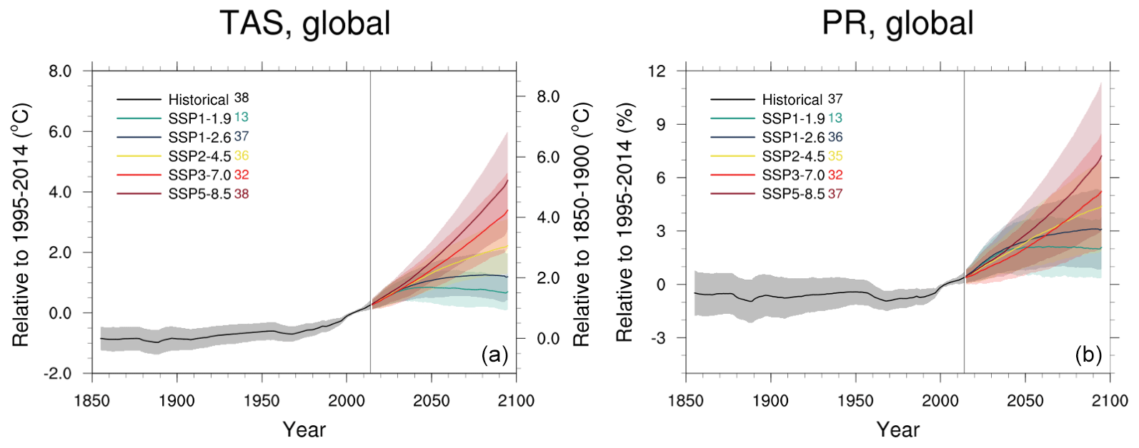
Figure 1(a) Global average temperature time series (11-year running averages) of changes from current baseline (1995–2014, left axis) and pre-industrial baseline (1850–1900, right axis, obtained by adding a 0.84 ∘C offset) for SSP1-1.9, SSP1-2.6, SSP2-4.5, SSP3-7.0 and SSP5-8.5. (b) Global average precipitation time series (11-year running averages) of percent changes from current baseline (1995–2014) for SSP1-1.9, SSP1-2.6, SSP2-4.5, SSP3-7.0 and SSP5-8.5. Thick lines are ensemble means (number of models shown in the legends). The shading represents the ±1.64σ interval, where σ is the standard deviation of the smoothed trajectories computed year by year (thus approximating the 5 %–95 % confidence interval around the mean of a normal distribution). Note that the uncertainty bands are computed for the anomalies with respect to the historical baseline (1995–2014). Thus, the right axis of the global temperature plot, showing anomalies with respect to pre-industrial values, applies to the ensemble means, not to the uncertainty bands, which would be narrowest over the period 1850–1900 if we were to calculate uncertainties on the basis of the models' output over that period, rather than by simply adding an offset uniformly. See Fig. A2 for land-only and ocean-only averages and Tables A3 and A4 for the values of changes at mid- and late century.
In order to characterize when pairs of scenarios diverge, we define separation as the first occurrence of a positive difference between two time series, one under the higher and one under the lower forcing scenarios, which is then maintained for the remainder of the century. This is similar to Tebaldi and Friedlingstein (2013, TF13 in the following), who used the first occurrence of a significant trend in the year-by-year differences, then justified by the RCPs under consideration, among which only the lowest (RCP2.6) flattened out over the century. In that case, the remainder of the RCPs considered followed an increasing trajectory, with differential rates of increase, therefore justifying the expectation that year-by-year differences would eventually show a significant and persisting trend. Among the new scenarios, at least two are expected to follow a flat trajectory, or even a slight peak and decline (SSP1-1.9 and SSP1-2.6), rendering the expectation of a trend in their differences untenable. We therefore adopt a slightly different definition here, and we also note that this definition would need to be modified if overshoot scenarios – crossing their reference as they decrease – were the main focus of this analysis. Also, this is not the only way to define separating scenarios, and other studies have applied different, but still fairly similar, definitions, e.g., recently, Marotzke (2019). We use time series of GSAT after applying a 21-year running mean, as we are concerned with differences in climate rather than in individual years, whose temperatures are affected by large variability (this is the part of the definition that takes the place of the consideration of long-term trends in TF13). We also need to choose a threshold at which we deem the difference “positive” and somewhat discernible (this takes the place of asking for a significant trend in TF13). To do so, we use the results in Tebaldi et al. (2015), where the regional sensitivities of temperature and precipitation to changes in global average temperature were quantified. According to that analysis, a 0.1 ∘C difference in 20-year means of GSAT was the lowest value at which a multi-model ensemble consistently had a positive fraction of the grid cells experiencing significant warming. In Table A5, we report the precise years when the ensemble means of the smoothed GSAT time series under the various scenario pairs separate according to this definition and, in parentheses, when the last of all individual models' pairs of trajectories separate, but of course those precise estimates would change if our choices of the moving window and the threshold had been different. The ensemble average trajectory of GSAT under SSP5-8.5 separates from the lower scenarios' ensemble average trajectories between 2027 and 2034, with the longer time as expected applying to the separation from SSP3-7.0. SSP3-7.0 separates from the two scenarios at the lower end of the range between 2031 and 2037, and 10 years later from SSP2-4.5. The ensemble average trajectory of global temperature under SSP2-4.5 separates from those under the two lower scenarios, SSP1-1.9 and SSP1-2.6, by 2034 and 2039, respectively, while the ensemble average GSAT trajectories under the two lower scenarios, SSP1-1.9 and SSP1-2.6, separate from one another in 2042 (in Fig. A3, the differences between ensemble averages for each pair of scenarios appear as red lines). When considering individual models' trajectories under the different scenarios and defining the time of separation when the last of all individual pair of trajectories separates, model structural differences and a larger effect of internal variability cause a significant delay compared to the ensemble mean separation. Depending on the pair of scenarios considered, the length of the delay necessary for the last of the models to show separation varies significantly: as few as 6 years for the full separation of SSP1-2.6 from SSP5-8.5 and as many as 19 years for the full separation of SSP3-7.0 from SSP5-8.5 (Fig. A3, black lines, and values in parentheses in Table A5).
Ensemble mean precipitation change by 2081–2100 (as a percentage of the 1995–2014 baseline) is between 2.0 % and 3.0 % for the lowest scenarios (SSP1-1.9 and SSP1-2.6), 4.2 % and 4.9 % for SSP2-4.5 and SSP3-7.0, and 7.3 % for SSP5-8.5. As expected, the larger variability of precipitation changes (relative to temperature changes), both from internal sources and model response uncertainty, is such that only the highest scenario ensemble mean trajectory separates from the lower ones appreciably before 2050, while the lowest scenario separates from the rest around mid-century. The ensemble means of the three scenarios in between overlap until close to 2070. The multi-model spread and internal variability confound a large fraction of the individual scenarios' trajectories until the end of the century (Fig. 1b). Both the magnitude of the changes and their variability are larger for precipitation averages over land than over oceans (Fig. A2; see also Table A4 for a complete list of mid- and late-century changes).
3.1.2 Normalized patterns
In Fig. A4, we show ensemble average patterns of change by the end of the century under the five scenarios for both variables. In this section, we focus our discussion on the general features emerging from the average normalized patterns. Normalized patterns are computed as the end-of-century (percent) change compared to the historical baseline, divided by the corresponding change in global mean temperature. This computation is first performed for each individual model or scenario, at each grid point, after regridding temperature and precipitation output to a common grid. The individual normalized patterns are then averaged across models and the five scenarios. As we will show, the total variations among the population of normalized patterns that form this grand average are mainly driven by intermodel variability rather than interscenario differences. Thus, we choose to synthesize patterns of change across all scenarios by presenting regional changes per degree of global warming. More in-depth analyses, also exploiting complementary experiments from LUMIP and AerChemMIP, may provide a more refined view of the interscenario differences possibly arising from different regional forcings.
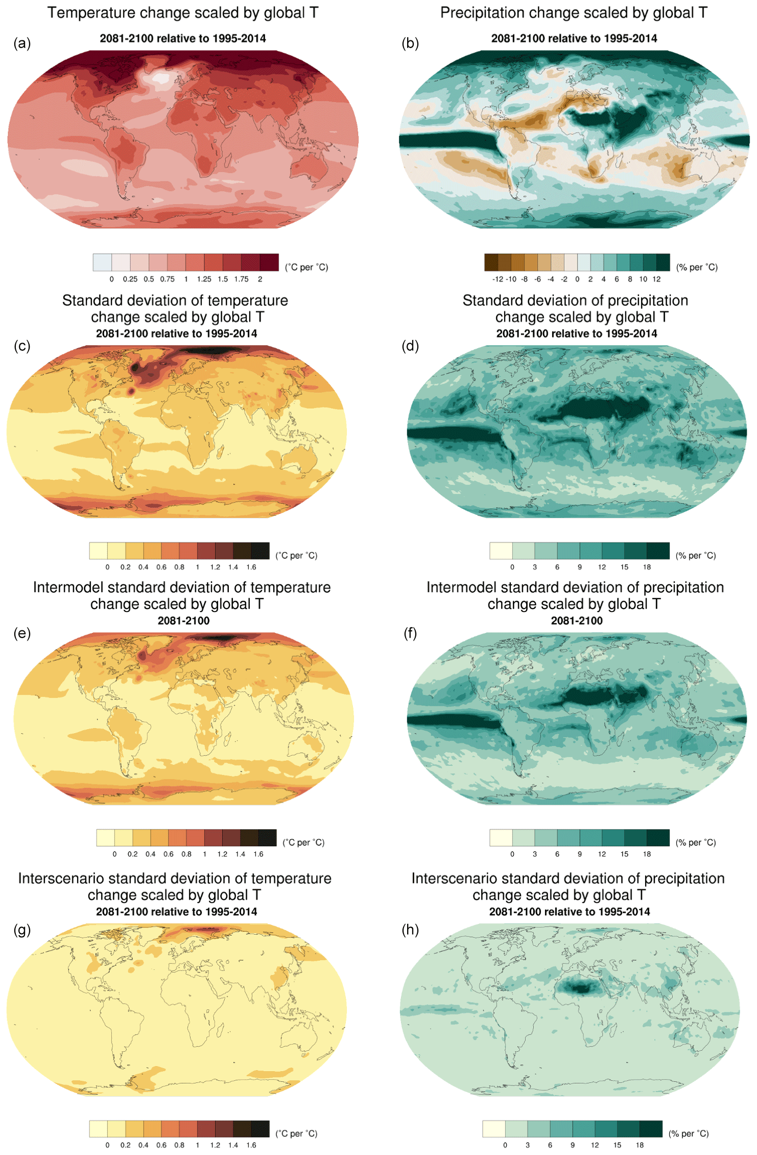
Figure 2(a, b) Patterns of temperature (a) and percent precipitation change (b) normalized by global average temperature change (averaged across CMIP6 models and all Tier 1 plus SSP1-1.9 scenarios). (c, d) Standard deviation of normalized patterns for individual CMIP6 models and scenarios. The individual patterns are the elements from which the averages shown in the top row are computed. (e, f) Standard deviation of normalized patterns, after averaging across scenarios, highlighting the role of intermodel variability. (g, h) Standard deviation of normalized patterns after averaging across models, highlighting the role of interscenario variability.
Figure 2 (top row) shows the spatial characteristics of warming and of wetting and drying. For temperature changes, the left panel confirms the well-established gradient of warming decreasing from northern high latitudes (with the Arctic regions warming at twice the pace of the global average) to the Southern Hemisphere and the enhanced warming in the interior of the continents compared to ocean regions (which consistently warm slower than the global average). This differential is particularly pronounced in the Northern Hemisphere (and would be muted if the normalized pattern was computed at equilibrium). The familiar cooling spot in the northern Atlantic appears as well – the only region with a negative sign of change. Studies have suggested that the cooling signal is an effect of the slowing of the Atlantic Meridional Overturning Circulation, which creates a signal of slower northward surface-heat transport, resulting in an apparent local cooling (Caesar et al., 2018; Keil et al., 2020).
For precipitation, the strongest positive changes are in the equatorial Pacific and the highest latitudes of both hemispheres, especially the Arctic region. The large changes in subtropical Africa and Asia are due more to the small precipitation amounts of the climatological averages in these regions (at the denominator of these percent changes) than to a truly substantial increase in precipitation (see also below for variability considerations). A strong drying signal continues to be projected for the Mediterranean together with central America, the Amazon region, southern Africa and western Australia.
Similar to Tebaldi and Arblaster (2014), we give a measure of robustness of these patterns by computing the standard deviation at each grid point across individual model or scenario patterns (Fig. 2, rows 2–4). We further distinguish the relative contribution of scenario and model variability by computing standard deviations after averaging across models separately for each individual scenario and across scenarios for each individual model, respectively. Figure 2, second row, highlights in darker colors regions where the standard deviation is higher and patterns are less robust. For temperature patterns, as has been found in earlier studies of pattern scaling (starting from Santer et al., 1990, and in more recent work, like Herger et al., 2015), the edges of sea ice retreat at both poles are areas where models disagree, and scenarios, in lesser measure, can be at odds due to their different timing of persistent ice melt. The variability and therefore uncertainty of the precipitation pattern mirrors the signal of change at low latitudes in the Pacific and over Africa and Asia. The comparison of patterns in the third and fourth rows of the figure elucidates the role of intermodel variability rather than scenario variability for both temperature and precipitation normalized changes, with scenario uncertainty only contributing to a small area of sea ice variability in the Arctic for temperature change and a subregion of the Sahara for precipitation change (where the denominator of the percentage values is small and therefore prone to cause instabilities in the values computed). Given the radically different sample sizes used to compute the averages from which scenario-driven standard deviations are derived compared to model-driven ones (more than 30 for the former and only five for the latter), we can also infer that internal variability is a likely contributor to model-driven standard deviation, while it is mostly eliminated before the computation of the scenario-driven standard deviation.
The robustness of these multi-model average patterns and the sources of their variability can be assessed by considering the same type of graphics computed from the four RCPs from the CMIP5 model ensemble.
Figures 3 (top row) and A5, using the same color scales, are easily compared to Fig. 2 and confirm the striking consistency of the geographical features of the normalized patterns, the size and spatial features of their variability, together with the components of the latter (i.e., model vs. scenario variability).

Figure 3Patterns of temperature (a) and percent precipitation change (b) normalized by global average temperature change (averaged across models and scenarios) from CMIP5 models and scenarios, for comparison with Fig. 2 (top row). Panels (c) and (d) show differences between CMIP6 and CMIP5 patterns.
We deem a rigorous quantification of the differences between patterns beyond the scope of this paper and focus on a qualitative assessment of the similarities that surface by showing in the bottom row in Fig. 3 the difference between CMIP6 and CMIP5 normalized patterns, confirming the small magnitude of the discrepancies in TAS over all regions, except for the Arctic, known to be affected by large variations among models, scenarios (with a possible role of the lowest scenario in CMIP6, SSP1-1.9, whose land–sea ratio has likely no equivalent among the CMIP5 scenarios, but further, more rigorous investigation is needed to confirm this) and internal noise (likely playing a minor role given the number of models and scenarios contributing to these averages). Similarly, for percent precipitation, the regions that stand out where the largest differences are found are the tropics, known to be affected by large variability and uncertainties. In this case, the possible role of aerosol forcing (Yip et al., 2011) warrants further investigation, especially as we consider that SSP3-7.0 forcing composition and trajectory are quite different from those of previous scenarios. As mentioned, the use of these experiments in conjunction with their variants by LUMIP and AerChemMIP could further attribute some of these scenario-dependent features to differences in regional forcing like land use or aerosols. Also, a subset of CMIP6 models are running the CMIP5 RCPs, and results from those experiments will allow a clean analysis of variance, partitioning sources between model and scenario generations.
3.1.3 Comparison of climate projections from CMIP6 and CMIP5 for three updated scenarios
In the previous section, the comparison of normalized patterns was by construction scenario independent. The design of ScenarioMIP, however, deliberately included scenarios aimed at updating CMIP5 RCPs, and three of those are in Tier 1. Updates in the historical point of departure (2015 for CMIP6 rather than 2006 for CMIP5) together with updates in the models forming the ensemble which reflect on the radiative forcing levels simulated by the individual models (Smith et al., 2020) are obvious differences that hamper a straightforward comparison. In addition, the emission composition of the scenarios also changed with the update, and we summarize how this occurred after presenting the projection comparison.
We show time series of global temperature for the three updated scenarios and the corresponding results from their CMIP5 counterparts: SSP1-2.6 vs. RCP2.6, SSP2-4.5 vs. RCP4.5 and SSP5-8.5 vs. RCP8.5 from CMIP6 and CMIP5, respectively. We show warming relative to the same historical baseline of 1986–2005 used by CMIP5 (Taylor et al., 2012) and to 1850–1900. We further show how observational constraints applied to the range of trajectories from the new models based on recently published work (Tokarska et al., 2020) result in lower and narrower projections at the end of the century and have the effect of bringing CMIP6 projections in closer alignment to CMIP5 end-of-century warming, even when the same type of constraints are applied to the latter.
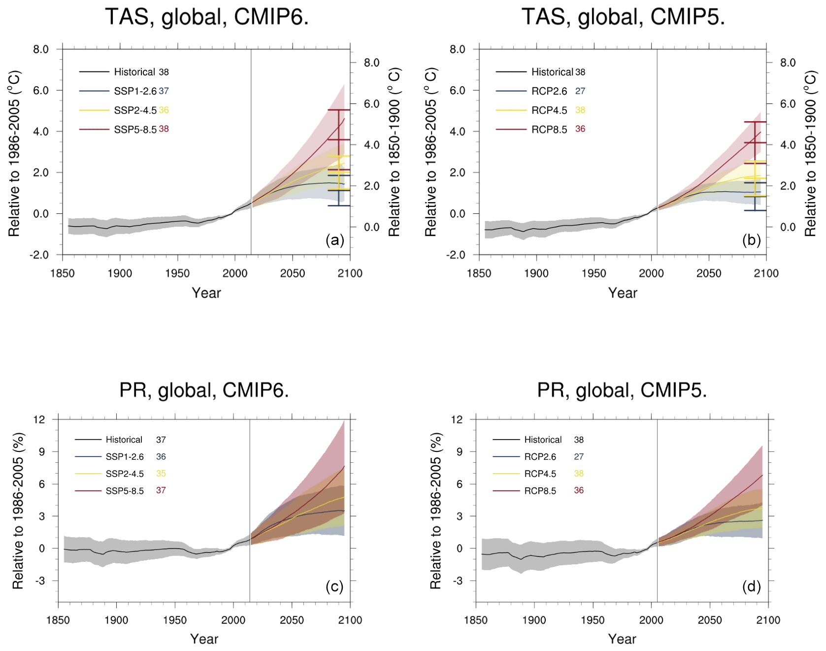
Figure 4Comparison of the three SSP-based scenarios updating three CMIP5-era RCPs with the corresponding CMIP5 output: SSP1-2.6, SSP2-4.5 and SSP5-8.5 (a, c) can be compared to RCP2.6, RCP4.5 and RCP8.5 (b, d) for global average temperature change (a, b) and global average precipitation change (c, d) (as a percentage of the baseline values, which are set to 1986–2005 for both ensembles). Indicators along the right axis of the plots of temperature projections show constrained ranges at 2100, obtained by applying the method of Tokarska et al. (2020). Note that, as in Fig. 1, the uncertainty bands in all figures are computed for anomalies with respect to the historical baseline (1986–2005 in this case). Thus, the right axis of the global temperature plots, showing anomalies with respect to pre-industrial values, applies to the ensemble means, not to the uncertainty bands, which would be narrowest over the 1850–1900 baseline, were they calculated using the data from simulations over that period, rather than being registered to the new axis only on the basis of the offset. Figure A6 shows a more direct comparison of the CMIP6 and CMIP5 ranges before and after the application of constraints at 2081–2100, and Table A6 lists those ranges (and the unconstrained percent precipitation changes for the same comparisons) at 2041–2060 and 2081–2100.
Figure 4 aligns two pairs of plots showing time series of global temperature and percent precipitation changes under the three updated scenarios and the original RCPs, from the CMIP6 and CMIP5 ensembles, respectively: Fig. 4a and c show three of the trajectories already shown in Fig. 1 but as anomalies or percent changes from the period 1986–2005, i.e., the last 20 years of the CMIP5 historical period (Taylor et al., 2012). Figure 4b and d show CMIP5 results for the three corresponding RCPs (see Table A2 for a list of the models used), also using the 1986–2005 baseline. The right axis on the temperature plots allows an assessment of changes compared to the 1850–1900 baseline. Table A6 lists mid- and late-century changes for all model ensembles under the different scenarios. The new unconstrained results reach on average warmer levels and have a larger intermodel spread, especially when comparing SSP5-8.5 to RCP8.5. There is 0.46 (for the scenarios reaching 2.6 W m−2), 0.49 (for the 4.5 W m−2 scenarios) and 0.67 ∘C (for the 8.5 W m−2 scenarios) more mean warming, while the upper end of the shading for SSP5-8.5 reaches 1.5 ∘C higher than the CMIP5 results (Table A6). The larger warming resulting from the CMIP6 experiments is a combination of different forcings and the presence among the new ensemble of models with higher climate sensitivities than the members of the previous generations. The higher climate sensitivities in CMIP6 compared to CMIP5 (Meehl et al., 2020; Zelinka et al., 2020) become more critical for higher forcings, when the model response is more highly correlated to its climate sensitivity, explaining the differential in the higher warming across the range of new scenarios, with the largest difference evident for SSP5-8.5.
Several recent studies (Brunner et al., 2020; Liang et al., 2020; Nijsse et al., 2020; Ribes et al., 2021; Tokarska et al., 2020) constrain the ensemble projections according to the evaluation of the ensemble historical behavior. All studies find a strong correlation between the simulated warming trends over the observed historical period and the warming in SSP scenarios, which suggested constraining future warming using observed warming trends estimated from several observational products, and all come to similar results. Here, and in Table A6, we show how the 2081–2100 means for both CMIP5 and CMIP6 are changed as a result of applying constraints as in Tokarska et al. (2020). Also in Fig. A6, we show the same results but focus specifically on these 20-year means, before and after the application of the constraints. The resulting observationally constrained ranges bring CMIP6 projections closer to both the raw CMIP5 ranges and their constrained counterparts in both mean and spread (especially the upper bound). In other words, models that project the most warming by the end of the century tend to do the least well in reproducing historical warming trends for both ensembles, but the effect is much more pronounced for CMIP6 than CMIP5 models (see also Fig. A6). After constraints are applied, the difference in the mean changes by 2081–2100 is 0.29 for the two lower scenarios and 0.15 ∘C under SSP5-8.5/RCP8.5. The difference in the upper range under the latter scenario is reduced to 0.59 ∘C.
Global precipitation projections follow temperature projections (O'Gorman et al., 2012), and therefore we see (unconstrained) CMIP6 trajectories reaching higher percent changes than CMIP5 of just below 1 %. Consistent with the relatively larger means, the spread of trajectories for individual scenarios, which combines internal variability with model uncertainty, is larger for the new models and scenarios.
As mentioned, part of the differences described are due to forcing differences between the corresponding scenarios in CMIP5 and CMIP6. These are by design small in terms of aggregate radiative forcing, when radiative forcing is defined as Intergovernmental Panel on Climate Change fifth Assessment Report (IPCC AR5)-consistent total global stratospheric-adjusted radiative forcing (AR5-SARF). By this measure of forcing, scenarios differ by less than 6 % in 2100 for the SSP1-2.6/RCP2.6 pair, 5 % for the SSP2-4.5/RCP4.5 pair and around 0.3 % at 8.9 W m−2 for the SSP5-8.5/RCP8.5 pair. Differences over the full pathway from 2015 to 2100 are below 15 %, 5 % and 4 %, respectively. However, the literature in recent years has moved away from the AR5-SARF definition (in particular, Etminan et al., 2016; see also implementation in Meinshausen et al., 2020) towards the use of effective radiative forcing (ERF), which differs from AR5-SARF in that it includes any non-temperature-mediated feedbacks (see, e.g., Smith et al., 2020).
Given that CMIP5 and CMIP6 concentration pathways differ with respect to their composition across gases and other radiatively active species (Lurton et al., 2020, Fig. 1), whose respective ERFs can be very different despite a similar AR5-SARF, the similarity between RCP and SSP scenarios in terms of forcing deteriorates when moving away from an AR5-SARF definition. For example, in SSP5-8.5, the AR5-SARF contribution of CH4 is by 2100 about 0.5 W m−2 lower than in the CMIP5 RCP8.5 pathway. This is offset by the difference in CO2 AR5-SARF, where SSP5-8.5 is around 0.5 W m−2 higher. In contrast, these compensating effects do not hold any longer when using ERF. In fact, because ERF is higher than AR5-SARF for CO2 and even more so for CH4, the 2100 radiative forcing levels after which both the RCP and SSP are named are not met precisely anymore when measured by ERF. Another pronounced difference between the CMIP5 RCPs and the new generation of SSP-RCP scenarios is that the latter span a wider range of aerosol emissions and corresponding forcings. The main reason for this difference is a wider consideration of the possible development of air pollution policies, ranging from major failure to address air pollution in the SSP3-7.0 pathway to very ambitious reductions of air pollution in the SSP1-2.6, SSP1-1.9 and SSP5-8.5 pathways (Rao et al., 2017). All the CMIP5 RCPs followed by comparison a more “middle-of-the-road” pollution policy path. Last, the effective radiative forcing levels reached by both sets of pathways can be different – depending on each climate model processes – from their nominal AR5-SARF values labeling the pathway, usually obtained by running the emission pathways through simple models, like using the Model for the Assessment of Greenhouse Gas Induced Climate Change (MAGICC) in its AR5-consistent setup (Riahi et al., 2017). A recent study with the EC-Earth model finds that about half of the difference in warming by the end of the century when comparing CMIP5 RCPs and their updated CMIP6 counterparts is due to difference in effective radiative forcings at 2100 of up to 1 W m−2 (Wyser et al., 2020). Figure A7, adapted from Meinshausen et al. (2020), shows a breakdown of the comparison into the three main forcing agents among greenhouse gases (CO2, CH4 and N2O) from which the significant differences in the composition can be assessed. Next to the AR5-consistent SARF time series, we also show effective radiative forcing ranges under the SSPs for the end of the 21st century for comparison using a newer version of MAGICC (MAGICC7.3).
Here, we note that in an effort to make the comparison more direct, CMIP5 RCP forcings are available to be run with CMIP6 models, and several modeling centers have started – at the time of writing – these experiments, which have been added to the Tier 2 design of ScenarioMIP since the description in O'Neill et al. (2016). If enough models contribute these results, a cleaner comparison of the effects of the updated forcing pathways, controlling for the updated models' effect, will be possible. Preliminary results with the Canadian model, CanESM2, confirm the significant role of higher radiative forcings found with EC-Earth.
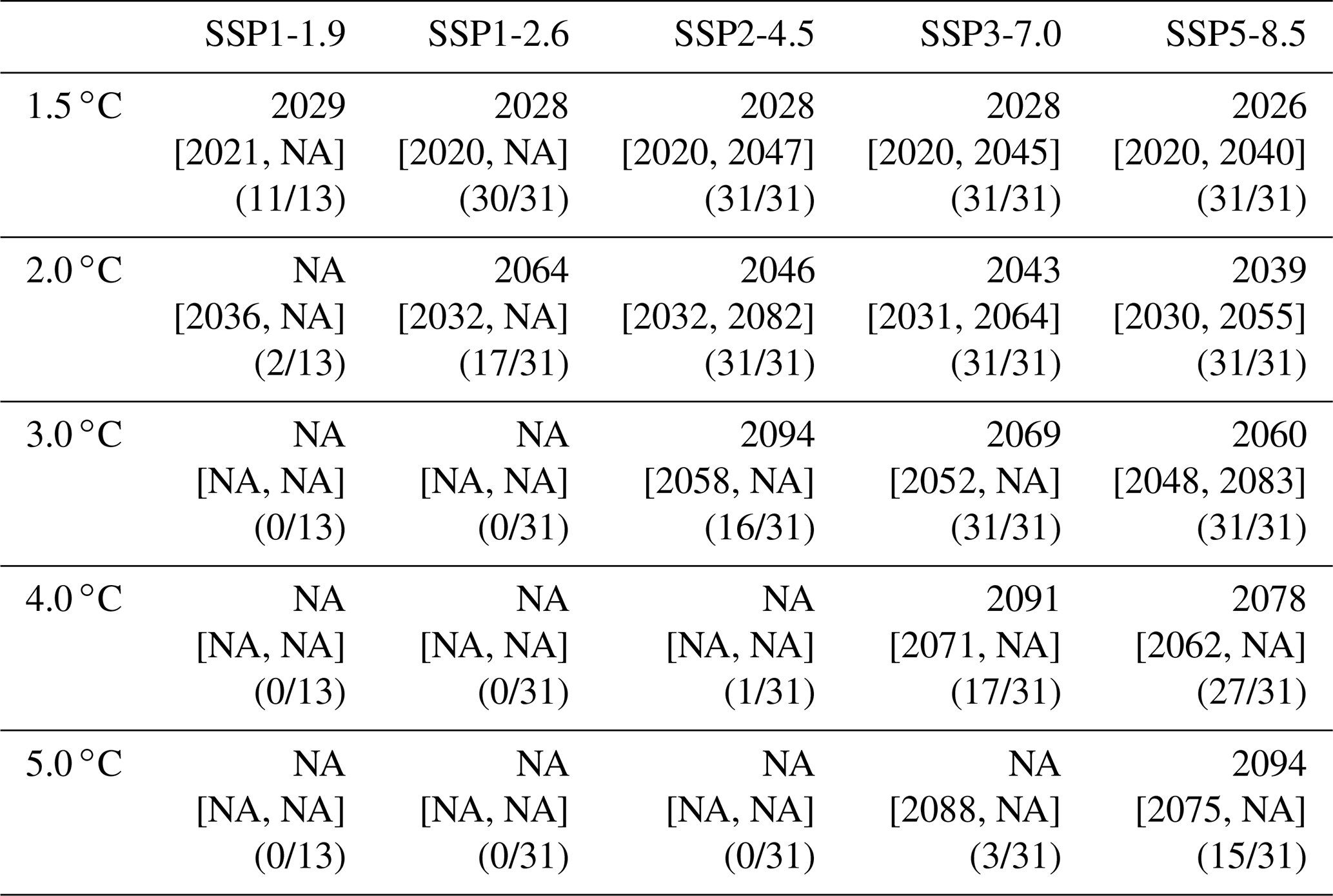
Table 1Times (best estimate and range – in square brackets – based on the 5 %–95 % range of the ensemble after smoothing the trajectories by 11-year running means) at which various warming levels (defined as relative to 1850–1900) are reached according to simulations following, from left to right, SSP1-1.9, SSP1-2.6, SSP2-4.5, SSP3-7.0 and SSP5-8.5. Crossing of these levels is defined by using anomalies with respect to 1995–2014 for the model ensembles and adding the offset of 0.84 ∘C to derive warming from pre-industrial values. We use a common subset of 31 models for the Tier 1 scenarios and all available models (13) for SSP1-1.9, while Table A7 shows the result of using all available models under each scenario. The number of models available under each scenario and the number of models reaching a given warming level are shown in parentheses. However, the estimates are based on the ensemble means and ranges computed from all the models considered (13 or 31 in this case), not just from the models that reach a given level. An estimate marked as “NA” is to be interpreted as “not reaching that warming level by 2100”. In cases where the ensemble average remains below the warming level for the whole century, it is possible for the central estimate to be NA, while the earlier time of the confidence interval is not, since it is determined by the warmer end of the ensemble range.
3.1.4 Scenarios and warming levels
The ever-increasing attention to warming levels as policy targets, also due to the recognition that strong relations are found between them and a large set of impacts, motivates us to identify the time windows at which the new scenarios' global temperature trajectories reach 1.5, 2.0, 3.0, 4.0 and 5.0 ∘C since 1850–1900. Table 1 shows the timing of first crossing of the thresholds by the ensemble average and the 5 %–95 % uncertainty range around that date. This is derived by computing the 5 %–95 % range for the ensemble of trajectories of GSAT and identifying the dates at which the upper and lower bounds of the range cross the threshold. The range is computed by assuming a normal distribution for the ensemble as the intermodel standard deviation multiplied by 1.64. Considering this range rather than the minimum and maximum bounds of the ensembles makes the estimates of the 5 %–95 % range more robust, especially for the lowest scenario (SSP1-1.9) for which we only rely on 13 models. The analysis is conducted after smoothing each of the individual models' time series by an 11-year running average to smooth interannual variability. The width of the intervals would change if constraints based on the observed warming trends were applied to the ensemble along the whole century (as shown in Fig. 4 for the end of the century), but here the unconstrained ensemble is used. The anomalies from 1850 to 1900 are computed as described in Sect. 3.1.1 by calculating anomalies with respect to the historical baseline (1995–2014) and then adding the offset value of 0.84 ∘C to minimize the effect of biases in the warming during the historical period of the different models. Note, however, that remaining differences between models and observations in the warming trends over the period 2014 to present, and the effects of differences between observed and projected forcings, may still introduce biases in the crossing level estimates, likely biasing them low.
We first synthesize results from the experiments from Tier 1, for which we extract a common subset of 31 models in order to make the threshold crossing estimates comparable across scenarios (for completeness, we document in Table A7 the behavior of all models available, which does not change qualitatively the results that we are about to describe).
The lowest warming level of 1.5 ∘C from pre-industrial values is reached on average between 2026 and 2028 across SSP1-2.6, SSP2-4.5, SSP3-7.0 and SSP5-8.5 with largely overlapping confidence intervals that start from 2020 as the shortest waiting time and extend until 2046 at the latest under SSP2-4.5. Note, however, that the lower bound of the ensemble trajectories (determining the upper bound of the projected years by which the level is reached) under SSP1-2.6 does not warm to 1.5 ∘C for the whole century (the NA as the upper bound of the time period signifies “not reached”). The next level of 2.0 ∘C is reached as soon as 13 years later by the ensemble average under SSP5-8.5 and as late as 32 years later under SSP1-2.6, a striking reminder of how different the pace of warming is in these scenarios. The confidence intervals have similar lower bounds between 2030 and 2032 and extend to 2077 for SSP2-4.5, while they are significantly shorter for the higher scenarios (2064 and 2054 for SSP3-7.0 and SSP5-8.5, respectively). The confidence intervals for SSP1-2.6 do not reach any of the higher warming levels, while by 2059 the ensemble average under SSP5-8.5 has already warmed by 3 ∘C. SSP3-7.0 takes 9 more years, while it takes until 2092 for the ensemble average under SSP2-4.5 to reach 3 ∘C. Under this scenario, it is worth noting that only 21 out of 37 models reach that level. Only the ensemble means of the two higher scenarios reach 4 ∘C, as early as 2077 for SSP5-8.5 and 14 years later for SSP3-7.0. The highest warming level considered of 5 ∘C is only reached by the upper range of SSP3-7.0 (only four models out of 33), while more than half the models running SSP5-8.5 (21 out of 39) reach that warming level in the last decade of the century (2094) as an ensemble average and as early as 2074 when the warmer end of the ensemble range is considered.
Only 13 models are available at the time of writing under the lowest scenario specifically designed to meet the Paris Agreement target of 1.5 ∘C warming by the end of the century. Of those, two remain below that target for the entire century, while others have a small overshoot of the target which was expected by design. The ensemble mean reaches 1.5 ∘C already by 2029. The lower bound never crosses that level, while the upper bound is already at 1.5 ∘C currently, i.e., by 2021 (as a reminder, CMIP6 future simulations start at 2015). In Table A8, a comparison of the CMIP5/CMIP6 three corresponding scenarios (SSP1-2.6, SSP2-4.5 and SSP5-8.5 compared to RCP2.6, RCP4.5 and RCP8.5) for a slightly larger ensemble of 36 CMIP6 models for which the three scenarios are available, and a CMIP5 ensemble of 29 models, shows dates compatible with the warmer characteristics of the CMIP6 models or scenarios. On average, the same target is reached from 3 to 9 years earlier by the CMIP6 ensemble means compared to the CMIP5 ensemble means. A more in-depth analysis than is in our scope is necessary to fully characterize the causes of this acceleration. Here, we note that the behavior of the CMIP6 ensemble means reflects the use of unconstrained projections, with equal weight given to high-climate-sensitivity models, which are often also those less adherent to historical trends and that may show a faster historical warming in the last decade or so than observed. In addition, as we discussed in the previous section, even scenarios having the same AR5-SARF label see different forcings at play. The result is to make the pace of warming faster, and, in several cases, a target that was not reached by the CMIP5 models under a given scenario is instead reached by the CMIP6 ensemble under the corresponding scenario. For example, 2.0 ∘C under SSP1-2.6 is reached in mean in 2056, while it was reached only by the upper bound (by 2040) under RCP2.6; at the opposite end, 5.0 ∘C was reached only by the upper bound (in 2083) under RCP8.5, while it is reached by the ensemble mean in 2093 under SSP5-8.5.
3.2 Climate projections from ScenarioMIP Tier 2 simulations
3.2.1 SSP3-7.0 initial condition ensembles
Five models (CanESM5, IPSL-CM6A-LR, MPI-ESM1-2-HR, MPI-ESM1-2-LR and UKESM1) contributed at least 10 initial condition (IC) ensemble members under SSP3-7.0. We focus here on the behavior of the ensemble spread over the 21st century, as measured by the values of the inter-realization standard deviations. In the following, the phrase “ensemble spread” is used, which has to be interpreted as the value of such standard deviation. Figure 5 shows the time evolution (over 1980–2100) of the ensemble spreads for global temperature and precipitation computed on an annual basis (a and b) and after smoothing the individual time series by an 11-year running mean (c and d). One of the models, CanESM5, provides 50 ensemble members that we use to randomly select subsets of 10 members and form a background “distribution” of the time series of ensemble spreads, shown in gray in Fig. 5. This is not meant to provide a quantitative assessment but rather a qualitative representation of the variability of “10-member ensembles”, which is what most models provide. When we compute trends for the time series of the temperature-ensemble spreads all show a negative slope, indicating that the ensemble spread has a tendency to narrow over time. In the case of the spread being computed among annual values, only two of the models pass a significance test at the 5 % level, while for decadal averages all models show significantly decreasing spreads (significantly negative trends). Trends of the ensemble spreads for precipitation are non-significant for all models when the spread is computed from annual values, while all are significantly negative, indicating a decrease in the spread, when that is computed from decadal means. This result appears robust for this small set of models, but confirmation with a larger number of models providing sizable initial condition ensembles will be important. Decreases in GSAT variability have however been found in earlier studies (Huntingford et al., 2013; Brown et al., 2017) and attributed to reduced Equator-to-pole gradients and reduced albedo variability due to the disappearance of snow and sea ice. A deeper investigation of the sources of changes in variability for both variables (which could also tackle how much of the change in precipitation variability is directly connected to that of GSAT and what other sources may be at play) is beyond our scope but will be facilitated by the availability of these CMIP6 IC ensembles in addition to the already-well-studied CMIP5-era large IC ensembles (Deser et al., 2020).
After detrending the values, we compare the distribution of the ensemble spreads for an individual model to that of other models in order to assess if models produce ensembles with spreads that are significantly different. We use a Kolmogorov–Smirnov test (at 5 % level) which measures differences in distribution. For several pairs of models, ensemble spreads based on annual values turn out to be indistinguishable: for temperature, CanESM5 ensemble spread is not significantly different from those of the MPI-ESM model at low resolution and those of the UKESM1 model. The latter in turn has an ensemble spread that is not different from that of the IPSL-CM model. For precipitation, CanESM5 and IPSL-CM produce comparable spreads, as do the two MPI-ESM models, and the MPI-ESM at low resolution compared to UKESM1. When we test the spreads of decadal means, all models appear significantly different from one another. Lastly, we can exploit the CanESM5 large ensemble in order to assess the number of ensemble members necessary to estimate the forced response of globally averaged TAS and PR, assuming that the mean response obtained by averaging the full ensemble of 50 member is representative of the true forced response. It is found that, for temperature, 10 ensemble members produce an ensemble mean trajectory indistinguishable from the one obtained averaging 50 members. For precipitation, only year-to-year variability is not completely smoothed out by averaging 10 rather than 50 ensemble members, but filtering by an 11-year running mean effectively cancels out annual “wiggles”.
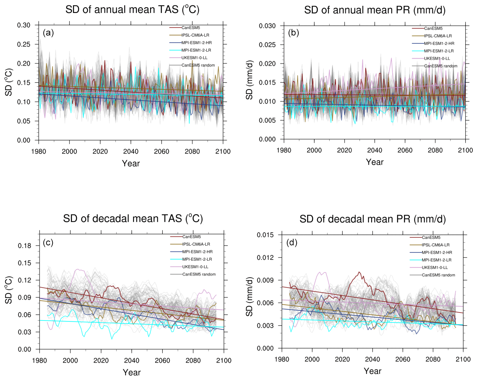
Figure 5Time series of ensemble spreads (i.e., inter-member standard deviations) computed at each year among annual (a, b) or decadal (c, d) mean values of TAS (a, c) and PR (b, d). The gray lines are obtained by resampling subset of 10 members from the CanESM5 model ensemble that provides 50 members. They are meant to provide a qualitative indication of the variability “hidden” in the 10-member ensembles provided by the majority of the models. The color lines show the time series of standard deviations computed from 10 members of five models running SSP3-7.0: CanESM5 (first 10 members, red), IPSL-CM6A-LR (yellow), MPI-ESM1-2-HR (blue), MPI-ESM1-2-LR (cyan) and UKESM1 (light purple). Straight lines show least-square fits of the linear trends.
3.2.2 Effects of mitigation policies comparing SSP5-8.5 with SSP5-3.4OS, and SSP4-6.0 with SSP4-3.4
The ScenarioMIP design includes two pairs of scenarios, each of which is derived from the same SSP and integrated assessment model and consists of one baseline scenario without mitigation and one scenario assuming mitigation policies that reduce radiative forcing. They can therefore be used to cleanly attribute differences in climate outcomes to mitigation efforts. The two sets of scenarios are SSP4-6.0 and SSP4-3.4 (produced with the Global Change Analysis Model (GCAM) model; Calvin et al., 2017) and SSP5-8.5 and SSP5-3.4OS (produced with the REgional Model of Investment and Development – Model of Agricultural Production and its Impacts on the Environment (ReMIND-MagPIE); Kriegler et al., 2017). Figures 6 and 7 show time series of global temperature and percent precipitation anomalies with respect to the baseline period of 1995–2014 for the two pairs, and the patterns of differences in temperature and percent precipitation change by the end of the century, which we can characterize as the benefits of mitigation within the two SSP worlds. For reference, the pattern of change for the lower scenario in the pair is also shown.
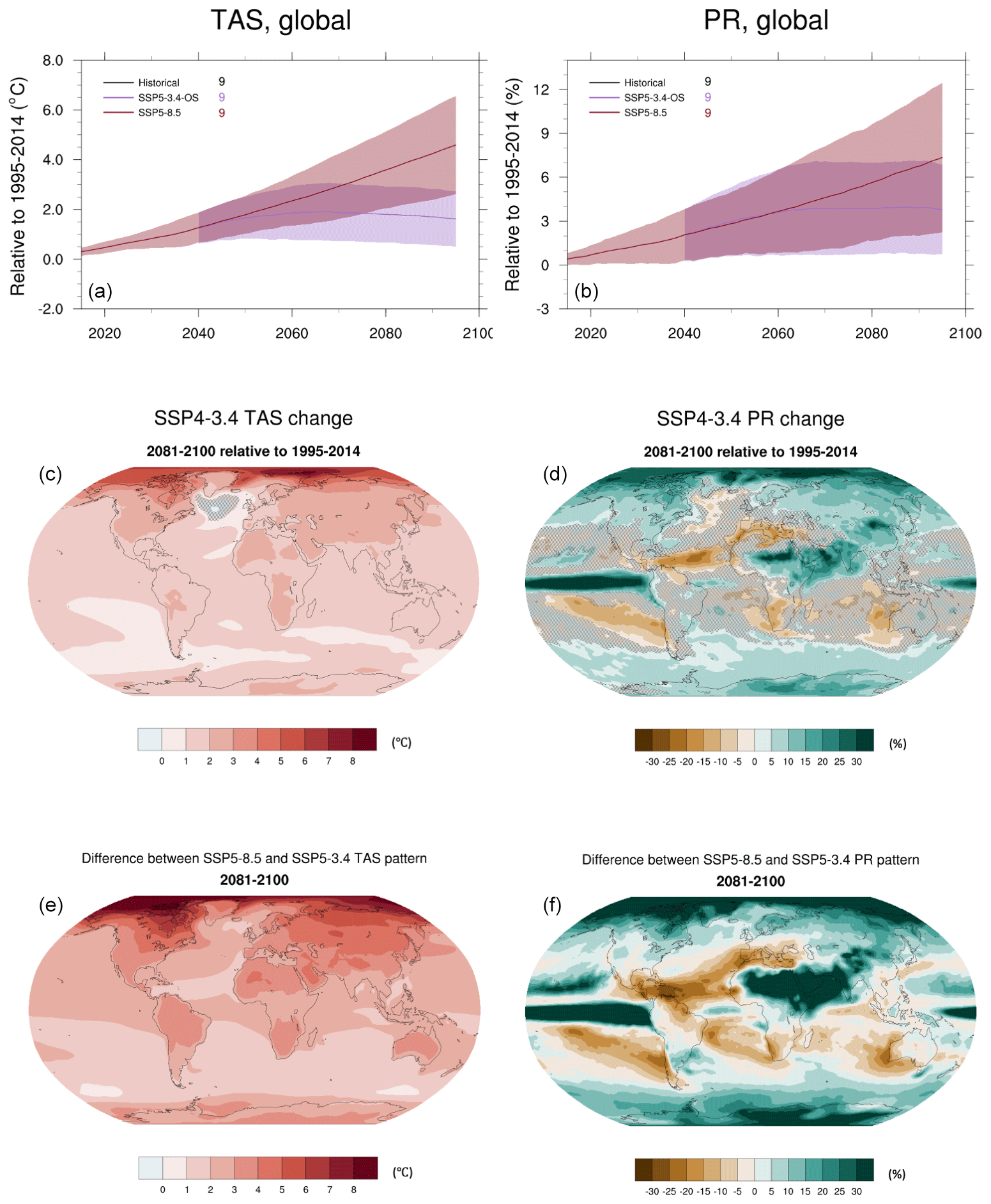
Figure 6Time series and patterns comparing SSP5-8.5 to SSP5-3.4OS. (a, b) Global average time series of temperature and percent precipitation change with respect to the 1995–2014 baseline (11-year running means). (c, d) Patterns of change for the same quantities, under the lower scenario, SSP5-3.4OS (stitched areas are not significant; i.e., the magnitude of the change does not exceed the models' standard deviation). (e, f) Differences between the patterns of change under the higher (SSP5-8.5) and lower scenarios.
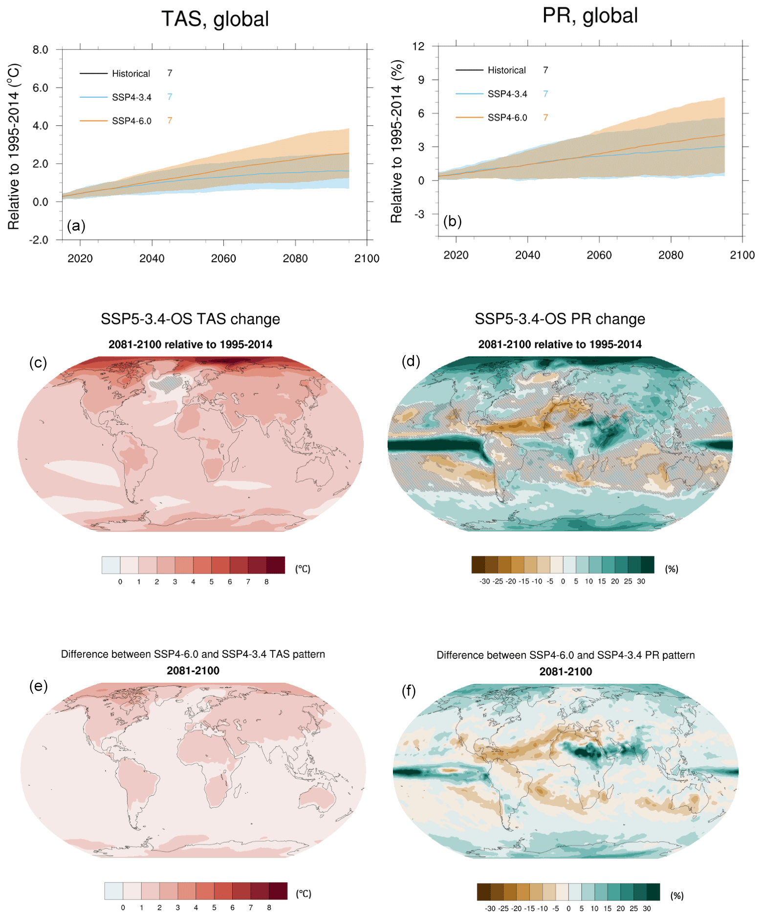
Figure 7Like Fig. 6 but for SSP4-6.0 and SSP4-3.4.
Figure 6 shows these outcomes for the pair of scenarios developed under SSP5. One of them is the unmitigated pathway already featured in the previous sections (SSP5-8.5), assuming high reliance on fossil fuels to support economic development and reaching 8.5 W m−2 by the end of the century. The other scenario (SSP5-3.4OS) follows the same path of emissions until 2040, when it enforces a steep decline in greenhouse gas emissions, which become negative after 2070 and therefore create an overshoot in concentrations, radiative forcing and global average temperature, to end up at 3.4 W m−2 at 2100. Note that the endpoint of this scenario, according to these global measures, coincides with the endpoint of SSP4-3.4, the lower scenario of the other pair considered in this section, which is however reached along a traditional non-exceed pathway.
Figure 7 shows results for the other pair, developed under SSP4, which by the end of the century reach 6.0 (without mitigation) and 3.4 W m−2 (with mitigation), respectively. Their greenhouse gas emissions start diverging immediately, by 2020, with those of the lower scenario already decreasing by that time, while those of the baseline scenario continue to increase for two more decades, plateauing and then decreasing only after 2060. Both scenarios have a non-decreasing shape in radiative forcing and temperature.
At global scales, Figs. 6 and A8a show that the forced temperature signals (identified by the ensemble averages, i.e., the red lines in the time series separation plots) for the SSP5-driven scenario pair respond within a decade of the divergence in the emission pathways; i.e., they separate by 2050 (just a couple of years later if we consider the last of the individual models) when we apply the same definition of separation used in Sect. 3.1.1. Global percent precipitation changes show the expected delay in the emergence of the mitigation signal, with ensemble average time series separating only after 2060 and the overlap of a large fraction of individual ensemble members under the two scenarios persisting until the end of the century. The corresponding time series in Fig. 7 (and Fig. A8b) shows that separation of temperature trajectories takes place even earlier for this pair of scenarios, by 2040 (2045 for the last of the individual models), consistently with the earlier start of the mitigation. A large majority of the precipitation trajectories still overlap at the end of the century.
The differential patterns of temperature and precipitation change have strikingly similar spatial features when comparing Figs. 6 and 7, only modulated by the strength of the changes, proportional to the gap in radiative forcings. Temperature changes benefit from mitigation over the whole globe but more significantly and increasingly so the higher the latitude in the Northern Hemisphere. All land regions see a benefit of mitigation (in terms of the forced signal, again represented by the difference in ensemble mean changes) of at least 2 to 3 ∘C in annual average temperatures at the end of the century, larger in most of the NH land regions and reaching 8 ∘C in the Arctic for the SSP5-3.4OS/SSP5-8.5 scenario pair. For precipitation changes, the larger differences translate in a more-than-doubled intensity (note that the colors are the same or stronger in the difference plot than in the scenario change plot) in both directions of change over the high latitudes (wetting) and the subtropics (drying). It is worth pointing out that patterns of change under the individual scenarios and patterns of differences between scenarios are similar, a further indication of the stable nature of the patterns of future change across different forcing scenarios.
Lastly, we use Figs. 6 and 7, together with Fig. A8c for an additional comparison, as the presence of two scenarios ending at the same level of radiative forcing (AR5-SARF), SSP4-3.4 and SSP5-3.4OS, allows us to compare the effects of the overshoot, after performing the same differencing for the six models that ran both of these scenarios. A comparison of the patterns of change under the two scenarios shows no apparent differences in the intensity of the changes for both temperature and precipitation, consistent with the global time series reaching a similar warming and precipitation change level at 2100. The model-by-model differences of these two scenarios (see Fig. A8c) for temperature show that the effects of the overshoot trajectory translate in warmer global temperatures starting from 2032 and all the way to 2080 in the ensemble mean and from 2038 to 2087 when considering the least differentiated of the individual models' pairs. The overshoot causes 0.4 ∘C of additional warming in the middle of the 2030–2080 period (2055), with a cumulative measure of differential warming over the period of about 14 degree years. This simple analysis suggests that average temperature and precipitation changes do not show significant memory and recover quickly after an overshoot of this magnitude.
The small number of models supporting these conclusions leaves the possibility that some of these numbers could change when larger multi-model ensembles will become available.
This paper provides an overview of ScenarioMIP results for surface temperature and precipitation projections under both Tier 1 and Tier 2 experiments, in addition to a comparison to CMIP5 outcomes for a subset of experiments that updated three of the RCPs.
The number of models contributing results for the simulations of 21st century scenarios ranges from almost 40 for experiments in Tier 1 to only 7 for some of the experiments in Tier 2. At the time of writing, the availability of the long-term simulations results is too scarce to provide a robust multi-model ensemble perspective, and we have not included those results.
Ensemble mean trajectories of global temperature under the Tier 1 and the 1.5 ∘C scenarios (SSP1-1.9, SSP1-2.6, SSP2-4.5, SSP3-7.0 and SSP5-8.5) span values between 0.7 and 4.0 ∘C above the historical baseline (1995–2014) (1.5–4.8 ∘C above 1850–1900 average), but individual models reach significantly larger warming levels under SSP5-8.5, above 5.5 ∘C (6.4 ∘C from 1850 to 1900). A comparison with the three CMIP5 RCPs (RCP2.6, RCP4.5 and RCP8.5) that reach the same nominal level of radiative forcing in 2100 (in terms of AR5-SARF) shows a wider range covered in the newest simulations, especially with respect to the upper end. Studies (Tokarska et al., 2020; Nijsse et al., 2020; Brunner et al., 2020; van Vuuren and Carter, 2014) have confirmed that this is attributable to an interplay of both higher radiative forcings by 2100 in the scenarios (when measured by the currently preferred metric, ERF) and higher climate sensitivities in a subset of the CMIP6 models, together with differences in background volcanic aerosols and greenhouse gases that make a straightforward comparison not possible (Fyfe et al., 2020; Lurton et al., 2020; Meehl et al., 2020; Meinshausen et al., 2020; Michou et al., 2020; Nicholls et al., 2020; Séférian et al., 2020; Smith et al., 2020; Wyser et al., 2020). We have shown that when applying constraints based on historical warming rates that weigh models differently on the basis of their performance (Tokarska et al., 2020), ensemble means and ranges of the CMIP6 experiments are brought closer to the corresponding means and ranges from CMIP5 model results, as many of the models with higher climate sensitivities also tend to perform less well over the historical period in terms of regional and aggregate warming trends (Brunner et al., 2020). This remains true even when the same constraints are applied to the CMIP5 ensembles, as they do not have as large an effect on the resulting trajectories (Figs. 4 and A6). A recent assessment performs a thorough attempt at constraining the distribution of climate sensitivity based on multiple lines of evidence, independently of climate models characteristics (Sherwood et al., 2020). If the resulting distribution of equilibrium climate sensitivity (ECS) were to be used to downweigh or cull models whose ECS is deemed an outlier, we would likely see changes in the CMIP6 ensemble projections in the same direction as those obtained by historical warming constraints, but formal studies applying this alternative type of constraint have not yet been published. The lack of a one-to-one correspondence between ECS and transient climate response (Sanderson, 2020), the latter more directly responsible for transient warming, further urges caution with this inference. According to the Tier 1 scenarios and SSP1-1.9, the 1.5 ∘C target (above 1850–1900) is reached by the model ensemble average in the second half of the current decade (between 2026 and 2029, depending on the scenario). The scenario decides if the 2.0 ∘C threshold is reached after only 13 more years (SSP5-8.5) or after more than 35 (SSP1-2.6), whereas it is never reached under SSP1-1.9. Only under SSP3-7.0 and SSP5-8.5 do a majority of models reach 4 ∘C, while 5 ∘C is reached by half of the ensemble members only under SSP5-8.5: models produce 4.0 ∘C of warming, on average, under the two higher scenarios in 2078 (SSP5-8.5) and 2091 (SSP3-7.0), while by 2094 5.0 ∘C is reached by the ensemble average under SSP5-8.5. Global precipitation change follows the pace and magnitude of warming (O'Gorman et al., 2012; Lambert et al., 2008) and spans a higher range of ensemble mean projections (by slightly less than 1 %) than CMIP5 and a wider range of variability around them. Time series computed separately for land and ocean regions, and global patterns of change – calculated as function of global warming – confirm well-established behaviors: warming is stronger over land than over oceans; the north-to-south warming gradient over the globe persists, with strong polar amplification signals resulting in projected warming at twice the pace of the global average in the Arctic region. The regional cooling effect of North Atlantic upwelling emerges clearly. Precipitation change appears stronger on average over land than over the globally averaged oceans, with the (by now familiar) multi-model mean patterns of wetting and drying, with the high latitudes and the equatorial Pacific seeing increases and the semi-arid regions of the Mediterranean, Australia and South Africa expecting further drying. As was the case for CMIP5 and previous multi-model ensembles, the average response across models is very robust to changes in the size and trajectory of well-mixed GHG forcings and therefore similar across scenarios. However, individual models' regional behavior may deviate from the average behavior significantly, especially in the regions of high internal variability, at the edges of sea ice melt for temperature and in the equatorial Pacific for precipitation.
The availability of 10 (or more) ensemble members under SSP3-7.0 prescribed under Tier 2 and completed by five models at the time of writing allows us to detect a tendency toward decreasing internal variability on decadal scales over time for both temperature and precipitation in all models (we note that several models have voluntarily provided initial condition ensembles of various sizes under other scenarios, but we have used one member only for those, which was all that was required for participation in ScenarioMIP). When considering annual frequencies, only two of the models show significantly decreasing spread and only for global temperature. The decadal-scale results appear at odds with recent studies that detected increased variability of precipitation with warming (Pendergrass et al., 2017; Yun et al., 2021) and call for in-depth studies of the sources and robustness of the behavior here described. For several pairs of models, ensemble spreads based on annual values turn out to be indistinguishable, while after computing running decadal means all models show significantly different spreads from one another, confirming that the representation of the climate system internal noise characteristics remains model dependent (Parsons et al., 2020). CanESM5 provides 50 members, and a subsampling of its ensemble confirms that 10 realizations are sufficient to robustly estimate the forced signal of global temperature and precipitation by their averages, consistently with studies that have recently sought to investigate the question of how large a large ensemble needs to be for such estimation of those quantities (Milinski et al., 2020).
Lastly, a new feature of ScenarioMIP's design builds on the matrix framework combining SSPs to different radiative forcing levels and therefore allows estimates of the benefits of mitigation for two pairs of scenarios: one pair under SSP4, the other under SSP5 and an evaluation of the path dependency of warming in the presence of an overshoot. The comparison of SSP5-8.5 to the overshoot pathway that departs from it in 2040 to strongly mitigate radiative forcing down to 3.4 W m−2 by 2100 (SSP5-3.4OS) shows that the warming and absolute changes in precipitation avoided through late mitigation in 2040 could be up to half the expected changes under the high scenarios at the end of the century. The comparison of the other pair (SSP4-6.0 and SSP4-3.4) shows a similar geography of avoided physical impacts but with smaller absolute differences, given the smaller reduction in radiative forcing between these two scenarios. We also compare the end points of SSP4-3.4, which follows monotonically increasing forcing over the century, and those of SSP5-3.4OS, which overshoots the late-century levels in radiative forcing and temperature and therefore reaches them from above. Both temperature and precipitation changes (averaged over the last 20 years of the 21st century) appear comparable in magnitude, suggesting a short memory of the climate system with respect to global average temperature and precipitation, at least after it exceeds the ultimate target for up to 5 decades, and by about 15 ∘C of cumulative differential warming, as in this comparison. We note, however, that other environmental dimensions of climate change (such as ocean acidification or sea level rise) are not as easily reversible, if at all (Tokarska et al., 2019; Schwinger and Tjiputra, 2018; John et al., 2015; Mathesius et al., 2015; MacDougall et al., 2015; Tokarska and Zickfeld, 2015).
A more general analysis of the time it takes for the various scenarios to see a significant separation of GSAT trajectories shows that the ensemble averages can show the climatological effects of mitigation (which we define as a persistent difference of at least a tenth of a degree) already within 15 years from the divergence of forcings when comparing SSP5-8.5 to the two lower scenarios (SSP1-1.9 and SSP1-2.6). “Adjacent” scenarios take longer to separate but they all do so, according to the ensemble means, by the mid-2040s. Individual pairs of trajectories from the ensemble members can take between about 5 and 20 years longer than the ensemble means (the longer period corresponding to the comparison between the two higher scenarios, SSP3-7.0 and SSP5-8.5).
We have limited this analysis to two variables and simple descriptive statistics of their behavior. The ScenarioMIP design together with the presence of complementary experiments in several other MIPs and of the richness of the archived data (Jukes et al., 2020) from the ESM simulations is going to provide the basis for many more in-depth analyses of the physical system behavior. This will be further supported by a subset of CMIP6 models that are running CMIP5 RCPs, thus enabling a rigorous separation of the sources of variation between the two generations of experiments. Importantly, the ScenarioMIP effort aims at supporting integrated analyses of Earth and human systems' responses to future changes. These studies will integrate socioeconomic changes described by SSPs with climate system changes characterized by ESM outcomes to assess risks and possible mitigation and adaptation response options. While we do not address the integration of ScenarioMIP outcomes in interdisciplinary studies within this overview, that integration remains the overarching motivation for ScenarioMIP coordinated effort.

Figure A1ScenarioMIP design (modified from O'Neill et al., 2020). White and colored boxes indicate achievable 2100 levels of forcings under the different SSPs. Gray areas are at the intersection of SSPs and radiative forcing levels that were not achievable by any of the IAMs employed to produce these scenarios.
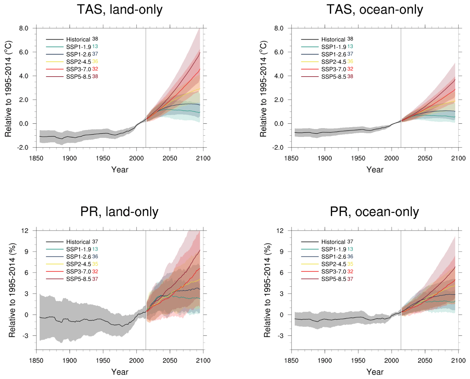
Figure A2Land-only and ocean-only average time series of temperature and percent precipitation changes relative to 1995–2014, for the four scenarios of Tier 1, SSP1-2.6, SSP2-4.5, SSP3-7.0, SSP5-8.5 and SSP1-1.9.
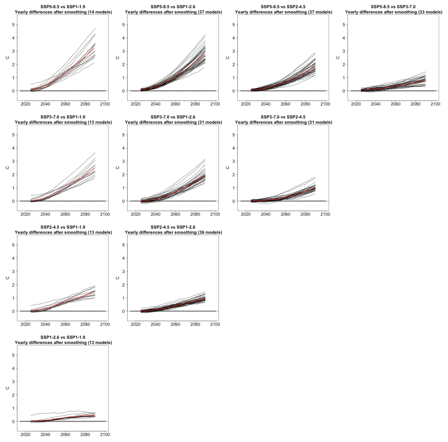
Figure A3Time series of year-by-year differences in GSAT between each scenario run in Tier 1 and each of the lower scenario runs (including SSP1-1.9). The time series from the individual models were first smoothed by a 21-year running mean. First row: differences between SSP5-8.5 and, respectively, SSP1-1.9, SSP1-2.6, SSP2-4.5 and SSP3-7.0. Second row: differences between SSP3-7.0 and, respectively, SSP1-1.9, SSP1-2.6 and SSP2-4.5. Third row: differences between SSP2-4.5 and SSP1-1.9 and SSP1-2.6. Fourth row: differences between SSP1-2.6 and SSP1-1.9. Each black line corresponds to an individual model's time series of differences. The red line is the ensemble mean difference. The ensemble size varies across the plots based on the number of models available for which the difference can be computed. It is as small as 10 members for those differences involving SSP1-1.9 and as large as 25 to 30 members when both scenarios belong to Tier 1.
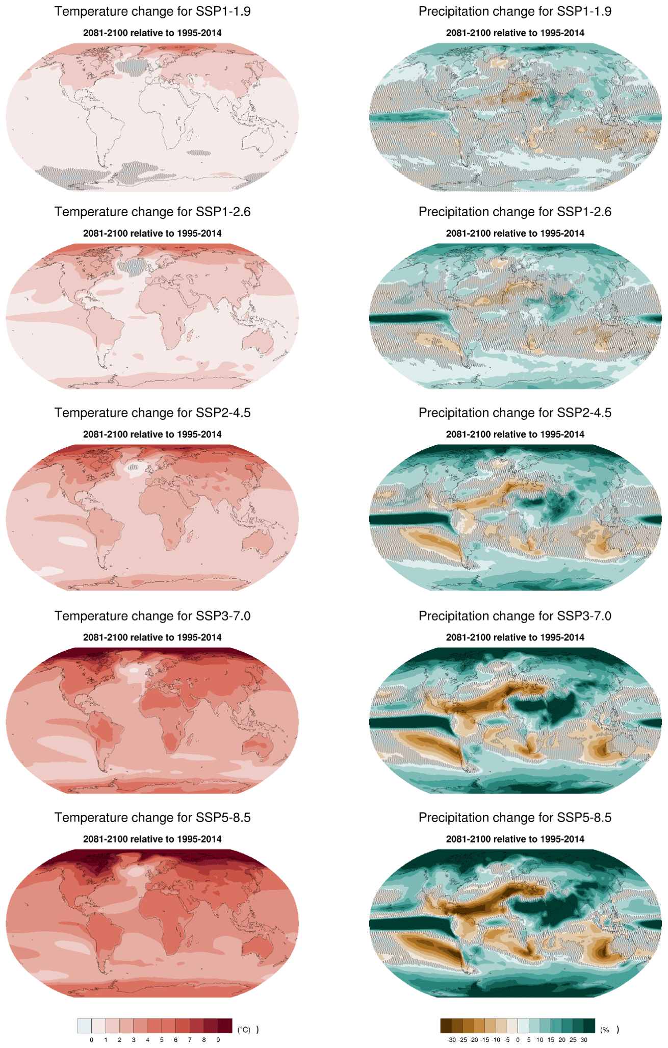
Figure A4Patterns of changes by 2081–2100 relative to 1995–2014 in surface air temperature (∘C) and precipitation (%) under the five scenarios. Stitched areas are not significant; i.e., the magnitude of the change does not exceed the models' standard deviation.
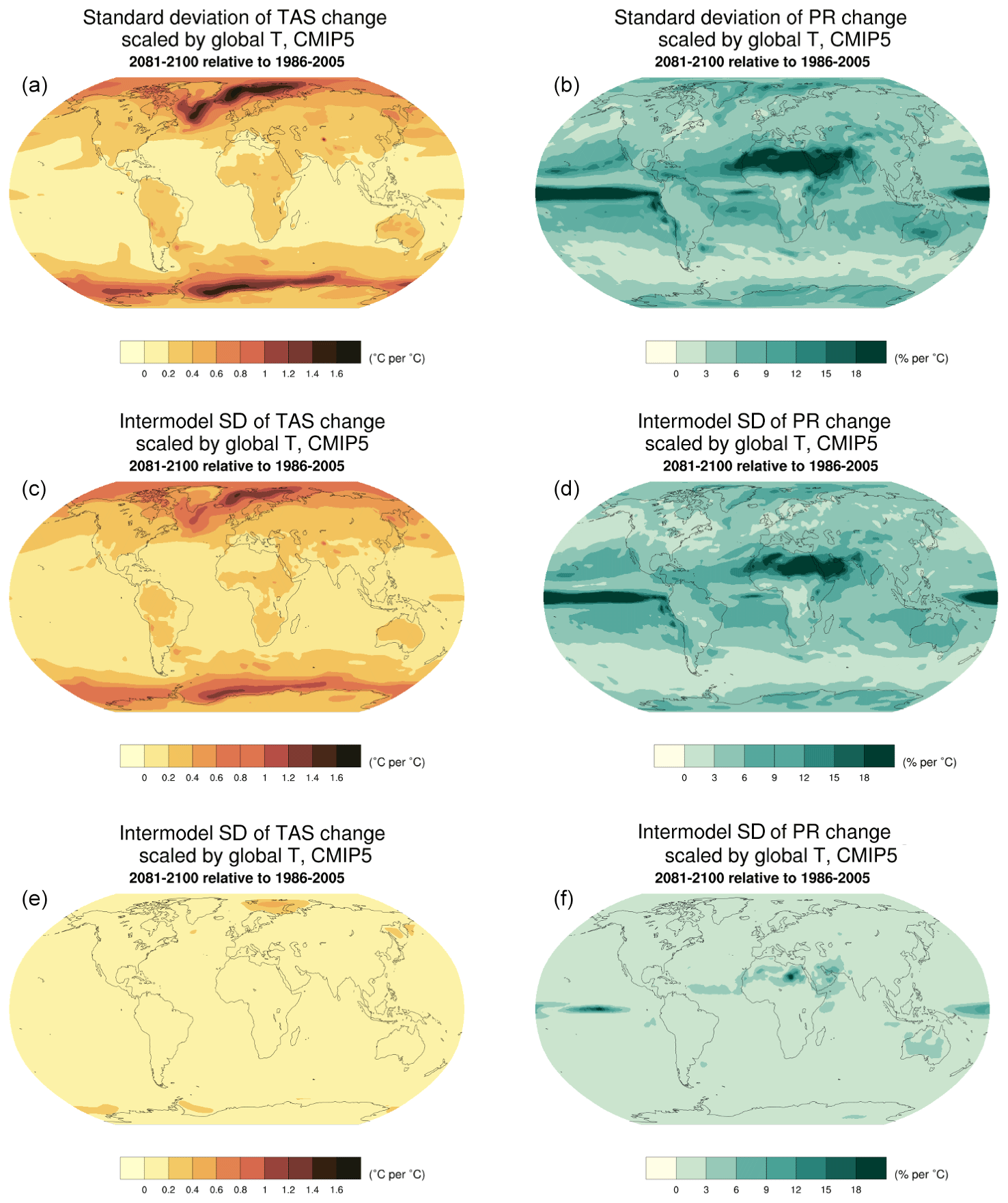
Figure A5(a, b) Standard deviation of normalized patterns for individual CMIP5 models and scenarios. The individual patterns are the elements from which the averages shown in Fig. 3 are computed. (c, d) Standard deviation of normalized patterns, after averaging across scenarios, highlighting the role of intermodel variability. (e, f) Standard deviation of normalized patterns after averaging across models, highlighting the role of interscenario variability. These standard deviations can be compared with the corresponding results from CMIP6 models and/or scenarios in Fig. A5.
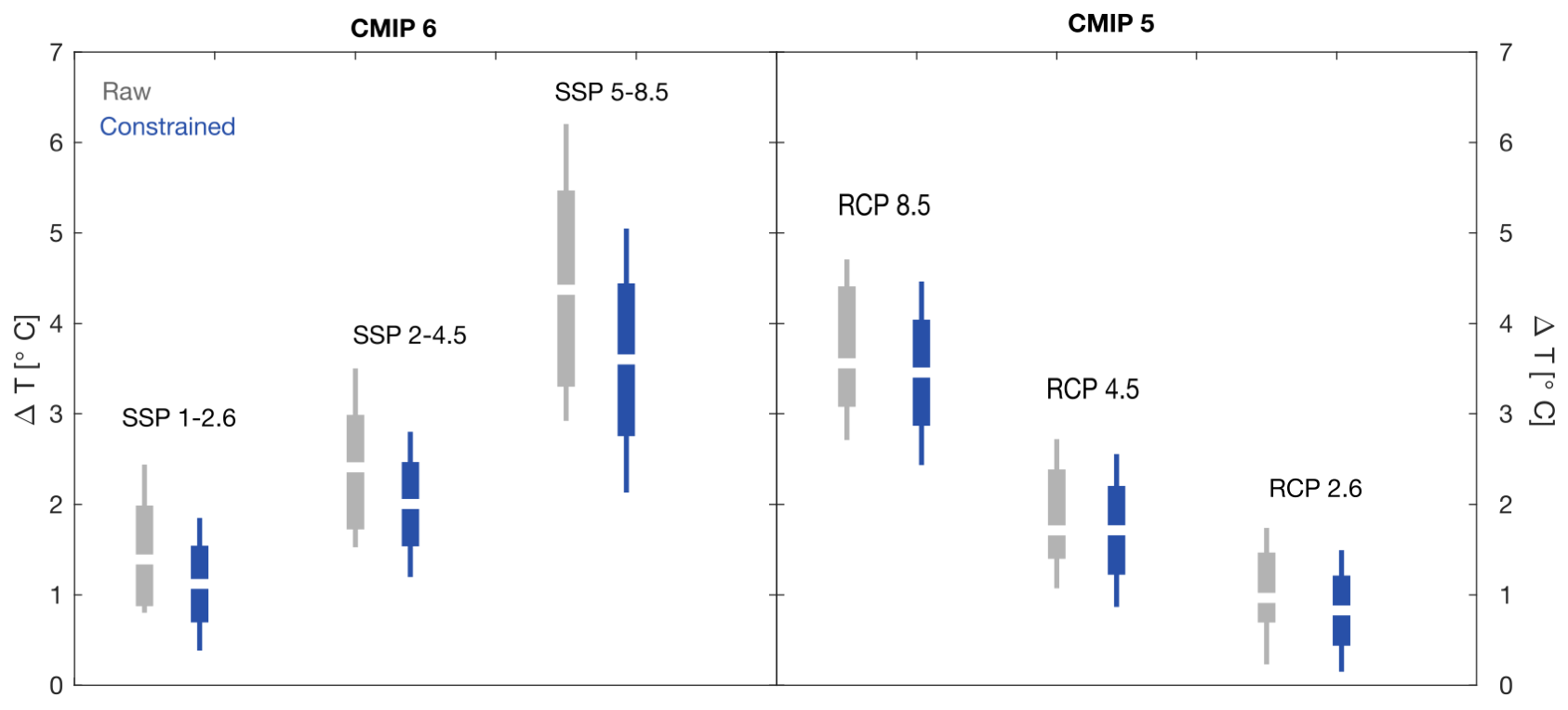
Figure A6A closer look at the effects of applying the Tokarska et al. (2020) constraints to CMIP6 and CMIP5 projections (mean changes at 2081–2100 compared to 1986–2005) for the nominally corresponding scenarios.
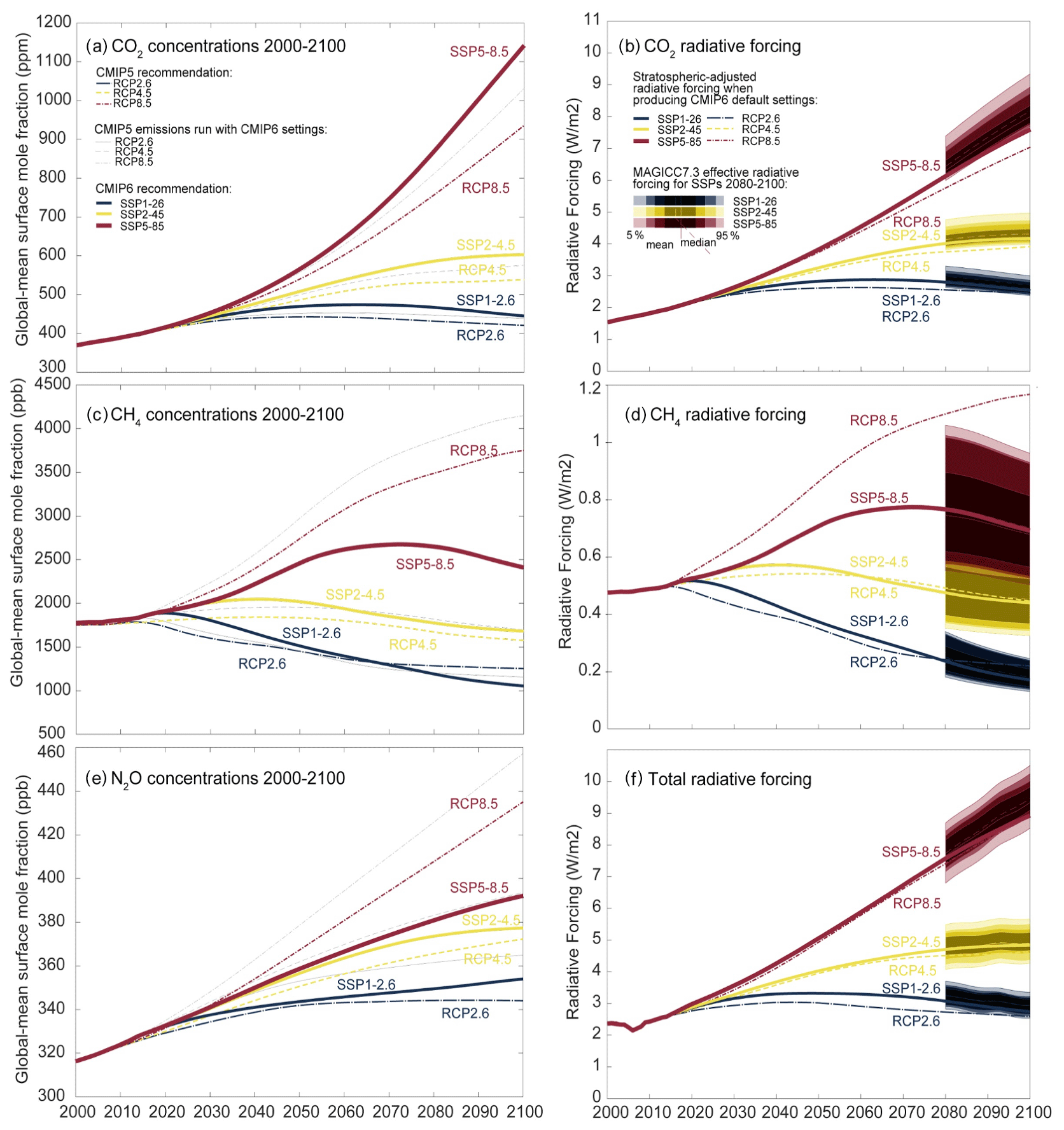
Figure A7Comparison of CO2, CH4 and N2O concentrations and radiative forcings for the concentration-driven CMIP5 runs with RCP-Y scenarios (Meinshausen et al., 2011) and CMIP6 runs with SSPX-Y scenarios (Meinshausen et al., 2020). The higher scenario (SSP5-8.5) features higher CO2 concentrations largely due to updated carbon cycle settings. RCP8.5 emissions with the same carbon cycle settings (shown as a thin dashed line in panel a) would produce similar CO2 concentrations. The methane and nitrous oxide concentrations are however lower in SSP5-8.5 than in RCP8.5 (despite updated gas cycles producing higher concentrations for the same emission trajectory). (a, c, e) Adapted from Fig. 11 in Meinshausen et al. (2020). At the time of producing the SSPs (March 2018), stratospheric-adjusted radiative forcings have been used to compare the nameplate radiative forcing levels in 2100 using MAGICC6.8 with IPCC-AR5-consistent settings; see panels (b, d, f). ERFs take additional adjustments into account that are non-temperature induced and differ from stratospheric-adjusted radiative forcings. Shown are 2080–2100 probabilistic results of SSP ERFs, using MAGICC7.3. These ERFs differ from SARFs and tend to be higher for CO2 and total radiative forcings; see panels (b, f). Given that the efficacy and rapid adjustments are different for different forcing agents, also the match between RCPs and SSP scenarios differs when comparing them in the effective radiative forcing space, rather than in terms of their stratospheric-adjusted radiative forcings.

Figure A8As in Fig. A3: year-by-year GSAT differences for the two pairs of scenarios differing only by the amount of mitigation assumed (a, b) and for the two scenarios that achieve the same level of radiative forcing by 2100, with one by overshooting it in the middle of the century (c). (a–c) Year-by-year differences for the seven models that ran SSP5-8.5 and SSP5-3.4OS, the seven models that ran SSP4-6.0 and SSP4-3.4, and the five models that ran SSP4-3.4 and SSP5-3.4OS. Black lines are differences computed between pairs of GSAT trajectories for each of the models. Red lines are differences between the two ensemble mean trajectories.
Table A1Modeling centers and their model(s) contributing to CMIP6 ScenarioMIP. The citations are included in the main bibliography. DOIs refer to the data available through the Earth System Grid Federation. The last columns details the experiments to which the model(s) contributed.
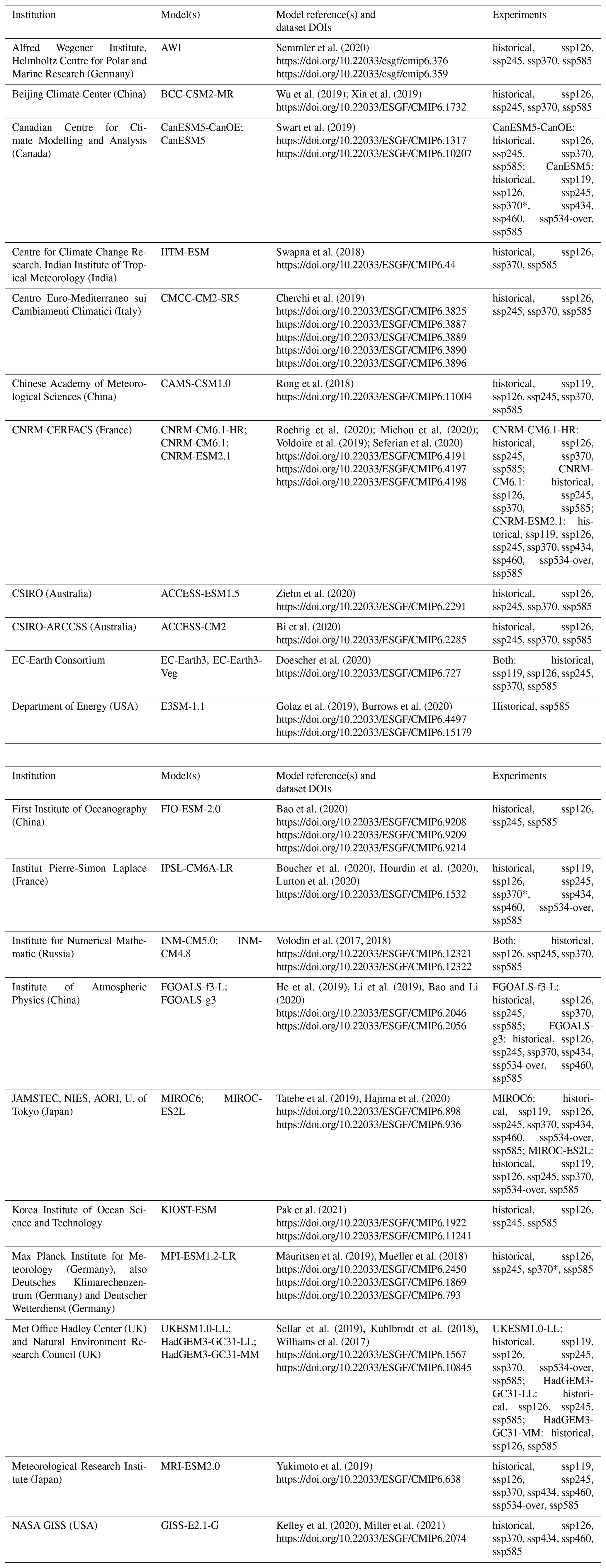
Table A2Modeling centers participating in CMIP5 and their models used in the comparison of SSPs and RCPs.
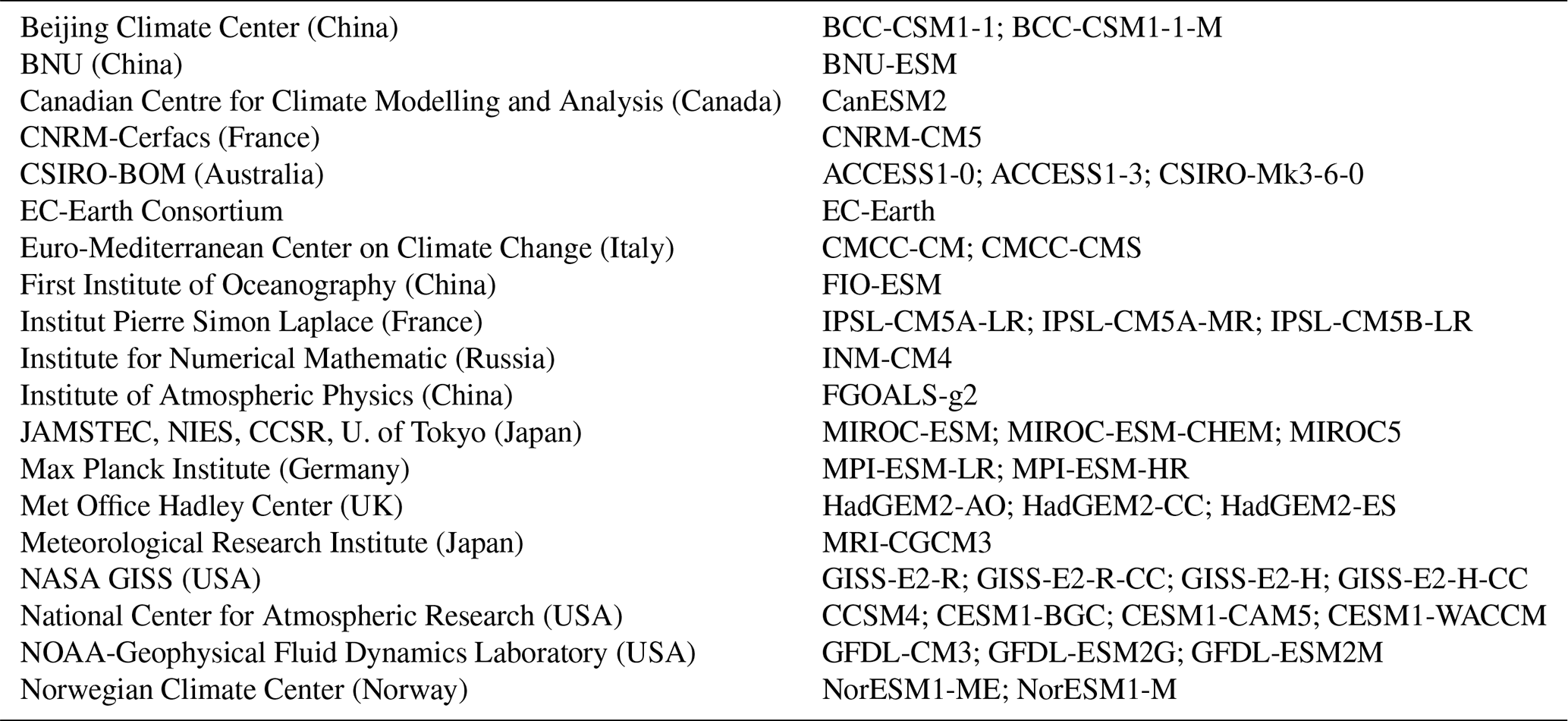
Table A3CMIP6 models' projected warming under the five scenarios by 2041–2060 and 2081–2100 relative to the historical baseline of 1995–2014. Ensemble mean values and, in square brackets, 5 %–95 % confidence intervals (±1.64σ).

Table A4CMIP6 models' projected changes in precipitation under the five scenarios by 2041–2060 and 2081–2100 expressed as percentages relative to the historical baseline of 1995–2014. Ensemble mean values and, in square brackets, 5 %–95 % confidence intervals (±1.64σ).
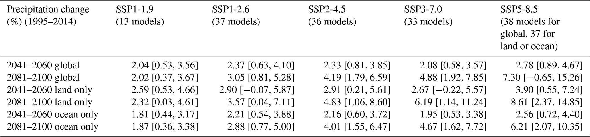
Table A5Time of separation between smoothed GSAT trajectories under pairs of scenarios. Shown are the years by which the ensemble means separate and, in square brackets, the years by which the last of the separation among individual models' trajectories takes place. Separation is defined as the emergence of a positive difference (we use 0.1 ∘C as the threshold) that persists for the remainder of the century. We first apply a 21-year running mean to the GSAT time series in order to characterize separation “of climates”.

Table A6Projected warming and precipitation change under comparable scenarios, for CMIP5 and CMIP6 ensembles, and for the CMIP6 ensemble constrained by the method of Tokarska et al. (2020). For the latter, the number of models remains the same as for the unconstrained projections. Differently from Tables A3 and A4, which use the CMIP6 current baseline period of 1995–2014, here all changes are relative to the CMIP5 current baseline period of 1986–2005. See also Fig. A6 for a graphical representation of the raw and constrained temperature projections for 2081–2100, besides Fig. 4 in the main text.
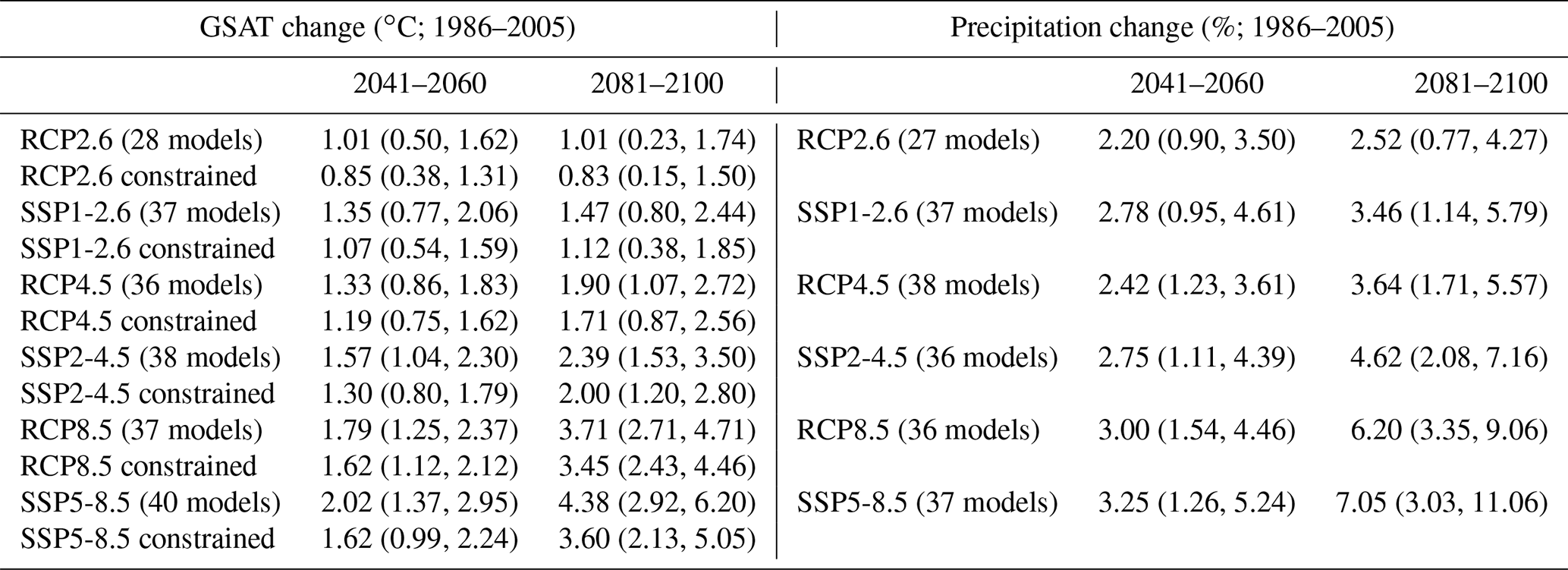
Table A7Like Table 1 in the main text: times of crossing of different warming levels by the available ensembles running the various scenarios (best estimate and range – in square brackets – based on the 5 %–95 % range of the ensemble after smoothing the trajectories by 11-year running means). Crossing of these levels is defined by using anomalies with respect to 1995–2014 for the model ensembles and adding the offset of 0.84 ∘C to derive warming from pre-industrial values. Since the number of models available under each scenario varies, and in some cases not all models reach a given warming level, those numbers are shown in parentheses. However, the estimates are based on the ensemble means and ranges computed from the whole ensemble, not just from the models that reach a given level. An estimate marked as “NA” is to be interpreted as “not reaching a given level by 2100”. In cases where the ensemble average remains below the warming level for the whole century, it is possible for the central estimate to be NA, while the earlier time of the confidence interval is not, since the upper bound of the ensemble range may still reach that warming level.
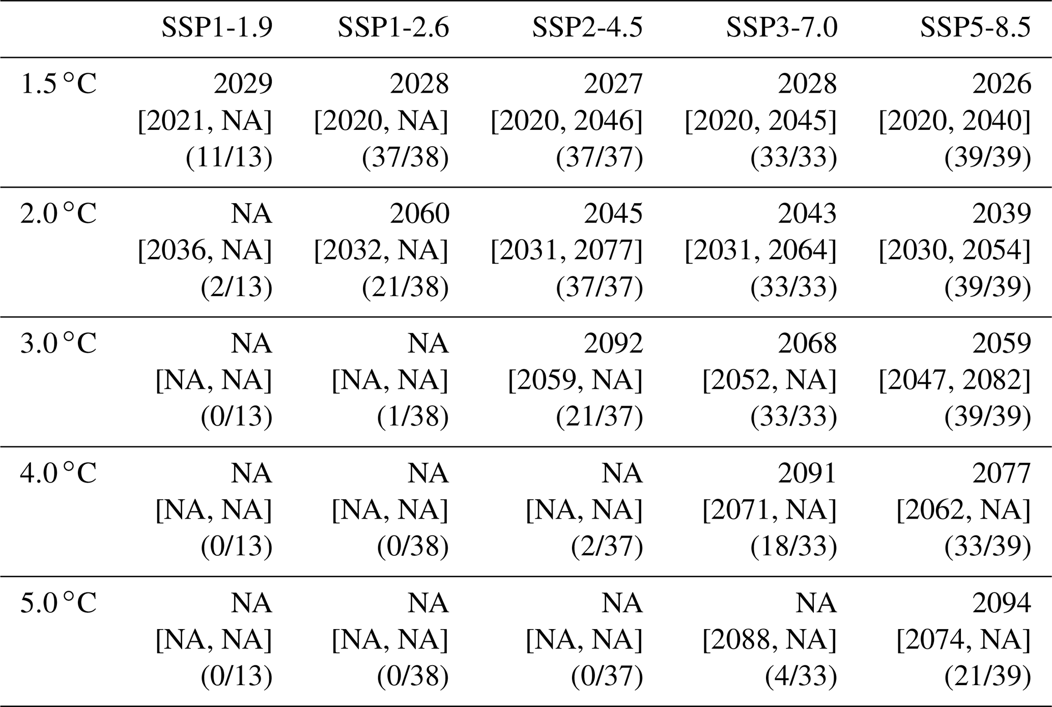
Table A8Warming level crossings for CMIP5 and CMIP6 scenarios/ensembles. Shown are times when an 11-year running average of the ensemble mean trajectory, and the lower and upper bounds of its 90 % confidence interval (1.64σ, where σ is the ensemble standard deviation after smoothing) cross various warming levels, under the three comparable scenarios: SSP1-2.6, SSP2-4.5 and SSP5-8.5 for CMIP6 models, RCP2.6, RCP4.5 and RCP8.5 for CMIP5 models. NA values indicate that the corresponding ensemble metric (mean, lower or upper bound of the confidence interval) does not reach the corresponding warming level by 2100. The numbers on the bottom row of each cell indicate the number of models that reach that warming level. The largest ensemble available under all three scenarios considered is used in both cases, with 36 CMIP6 models and 29 CMIP5 models.
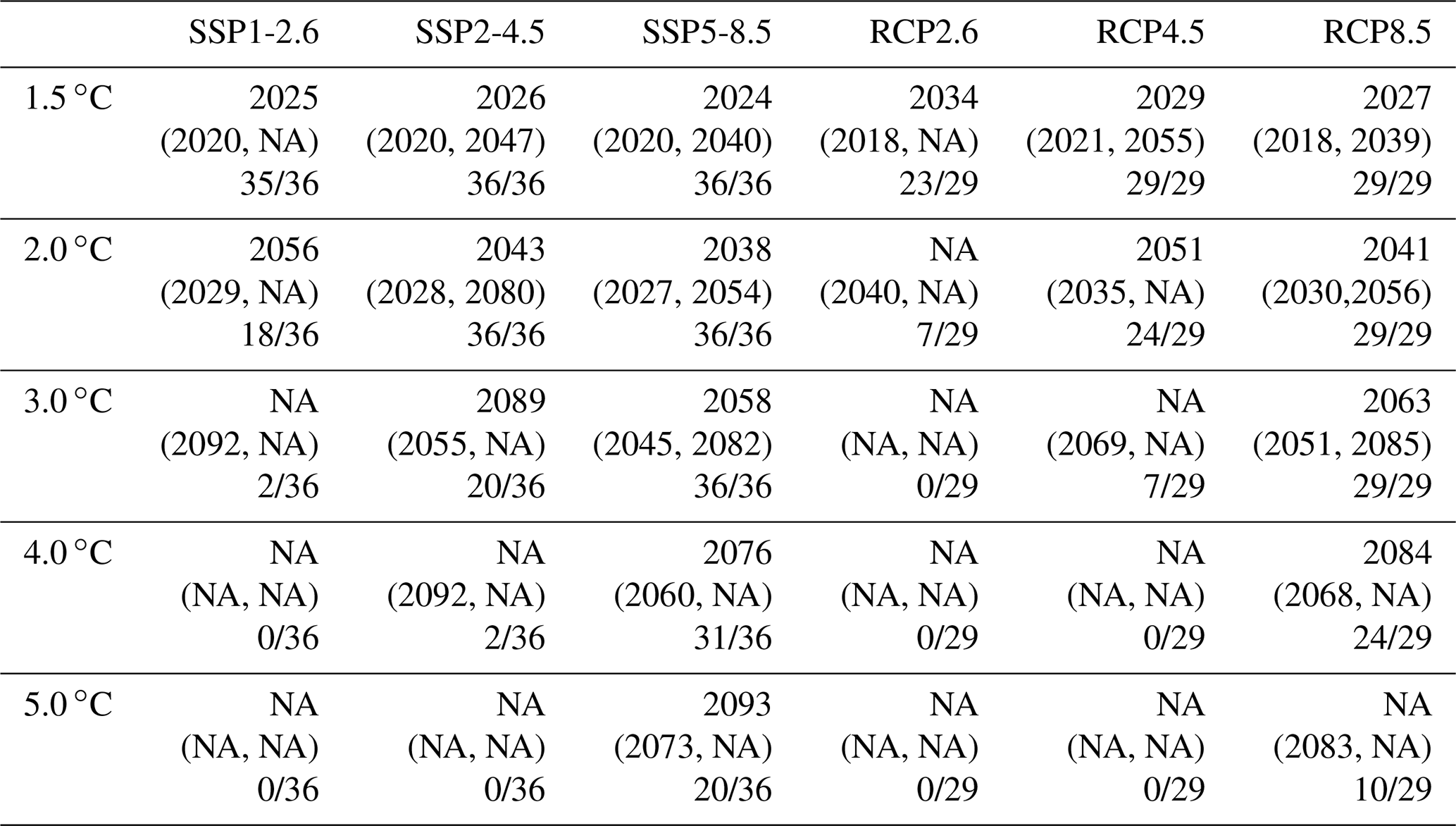
CMIP5 (see Table A2) and CMIP6 (see Table A1) model output is available through the Earth System Grid Foundation (ESGF) and can be directly used within the ESMValTool (e.g., https://esgf-data.dkrz.de/projects/esgf-dkrz/, last access: 7 January 2021) (ESGF, 2021). The corresponding recipe that can be used to reproduce the figures of this paper will be included in ESMValTool v2.0 (Righi et al., 2020; Eyring et al., 2020; Lauer et al., 2020; Weigel et al., 2020) as soon as the paper is published. ESMValTool (v2.1) is released under the Apache License, VERSION 2.0. The latest release of ESMValTool v2.1 is publicly available on Zenodo at https://doi.org/10.5281/zenodo.4300499 (Andela et al., 2020b). The source code of the ESMValCore package, which is installed as a dependency of ESMValTool v2.1, is also publicly available on Zenodo at https://doi.org/10.5281/zenodo.4525749 (Andela et al., 2020a). ESMValTool and ESMValCore are developed on the GitHub repositories available at https://github.com/ESMValGroup (last access: 7 January 2021) (ESMValGroup, 2021). As of December 2020, 27 modeling centers participated in ScenarioMIP by running at a minimum its Tier 1 experiments and provided their output through the ESGF. Table A1 lists them, together with their model(s) and the DOI referencing the data.
CT, VE, JF and EF designed and organized the analysis. KD performed data processing and analysis and drew all figures and most of the tables. CT wrote the first draft of the paper. All authors provided input, comments and editing on the various parts of the analysis. In addition, modeling center representatives (from SB to TZ in the authors' list) were responsible for performing the ScenarioMIP simulations and publishing their model output to the ESGF.
The authors declare that they have no conflict of interest.
We acknowledge the World Climate Research Programme (WCRP), which, through its Working Group on Coupled Modelling, coordinated and promoted CMIP. We thank the climate modeling groups (listed in Tables A1 and A2) for producing and making available their model output, the Earth System Grid Federation (ESGF) for archiving the data and providing access and the multiple funding agencies who support CMIP, ESGF and the individual modeling centers' efforts. Aurore Voldoire and Roland Séférian are grateful for the support of the team in charge of the CNRM-CM climate model. Supercomputing time was provided by the Météo-France/DSI supercomputing center. The computational resources of the Deutsches Klimarechenzentrum (DKRZ, Hamburg, Germany) that allowed the analysis of this study with the ESMValTool are kindly acknowledged.
Claudia Tebaldi was supported by the Energy Exascale Earth System Model (E3SM) project, funded by US Department of Energy, Office of Science, Office of Biological and Environmental Research. The Pacific Northwest National Laboratory is operated by Battelle for the US Department of Energy under contract no. DE-AC05-76RLO1830. This work has been also supported by the European Union's Horizon 2020 Framework Programme for Research and Innovation “Coordinated Research in Earth Systems and Climate: Experiments, kNowledge, Dissemination and Outreach (CRESCENDO)” project under grant agreement no. 641816 and the EVal4CMIP project funded by the Helmholtz Society. Work at LLNL was performed under the auspices of the US Department of Energy by Lawrence Livermore National Laboratory under contract no. DEAC52-07NA27344. Aurore Voldoire and Roland Séférian were supported by H2020 CONSTRAIN under the grant agreement no. 820829.
This paper was edited by Yun Liu and reviewed by two anonymous referees.
Andela, B., Brötz, B., de Mora, L., Drost, N., Eyring, V., Koldunov, N., Lauer, A., Predoi, V., Righi, M., Schlund, M., Vegas-Regidor, J., Zimmermann, K., Bock, L., Diblen, F., Dreyer, L., Earnshaw, P., Hassler, B., Little, B., and Loosveldt-Tomas, S.: ESMValCore (Version v2.2.0), Zenodo, https://doi.org/10.5281/zenodo.4525749, 2020a.
Andela, B., Brötz, B., de Mora, L., Drost, N., Eyring, V., Koldunov, N., Lauer, A., Mueller, B., Predoi, V., Righi, M., Schlund, M., Vegas-Regidor, J., Zimmermann, K., Adeniyi, K., Amarjiit, P., Arnone, E., Bellprat, O., Berg, P., Bock, L., Caron, L.-P., Carvalhais, N., Cionni, I., Cortesi, N., Corti, S., Crezee, B., Davin, E. L., Davini, P., Deser, C., Diblen, F., Docquier, D., Dreyer, L., Ehbrecht, C., Earnshaw, P., Gier, B., Gonzalez-Reviriego, N., Goodman, P., Hagemann, S., von Hardenberg, J., Hassler, B., Hunter, A., Kadow, C., Kindermann, S., Koirala, S., Lledó, L., Lejeune, Q., Lembo, V., Little, B., Loosveldt-Tomas, S., Lorenz, R., Lovato, T., Lucarini, V., Massonnet, F., Mohr, C. W., Pérez-Zanón, N., Phillips, A., Russell, J., Sandstad, M., Sellar, A., Senftleben, D., Serva, F., Sillmann, J., Stacke, T., Swaminathan, R., Torralba, V., and Weigel, K.: ESMValTool (Version v2.1.1), Zenodo, https://zenodo.org/record/4300499 (last access: 7 January 2021), 2020b.
Arora, V. K., Katavouta, A., Williams, R. G., Jones, C. D., Brovkin, V., Friedlingstein, P., Schwinger, J., Bopp, L., Boucher, O., Cadule, P., Chamberlain, M. A., Christian, J. R., Delire, C., Fisher, R. A., Hajima, T., Ilyina, T., Joetzjer, E., Kawamiya, M., Koven, C. D., Krasting, J. P., Law, R. M., Lawrence, D. M., Lenton, A., Lindsay, K., Pongratz, J., Raddatz, T., Séférian, R., Tachiiri, K., Tjiputra, J. F., Wiltshire, A., Wu, T., and Ziehn, T.: Carbon–concentration and carbon–climate feedbacks in CMIP6 models and their comparison to CMIP5 models, Biogeosciences, 17, 4173–4222, https://doi.org/10.5194/bg-17-4173-2020, 2020.
Bao, Q. and Li, J.: Progress in climate modeling of precipitation over the Tibetan Plateau, Natl. Sci. Rev., 7, 486–487, https://doi.org/10.1093/nsr/nwaa006, 2020.
Bao, Y., Song, Z., and Qiao, F.: FIO-ESM version 2.0: Model description and evaluation, J. Geophys. Res.-Oceans, 125, e2019JC016036, https://doi.org/10.1029/2019JC016036, 2020.
Bauer, N., Calvin, K., Hammerling, J., Fricko, O., Fujimori, S., Hilaire, J., Eom, J., Krey, V., Kriegler, E., Mouratiadou, I., Sytze de Boer, H., van den Berg, M., Carrara, S., Daioglou, V., Drouet, L., Edmonds, J. E., Gernaat, D., Havlik, P., Johnson, N., Klein, D., Kyle, P., Marangoni, G., Masui, T., Pietzcker, R. C., Strubegger, M., Wise, M., Riahi, K., and van Vuuren, D. P.: Shared Socio-Economic Pathways of the Energy Sector – Quantifying the Narratives, Global Environ. Change, 42, 316–330, https://doi.org/10.1016/j.gloenvcha.2016.07.006, 2017.
Beadling, R. L., Russell, J. L., Stouffer, R.J., Mazloff, M., Talley, L. D., Goodman, P. J., Sallée, J. B., Hewitt, H. T., Hyder, P., and Pandde, A.: Representation of Southern Ocean properties across Coupled Model Intercomparison Project generations: CMIP3 to CMIP6, J. Climate, 33, 6555–6581, https://doi.org/10.1175/JCLI-D-19-0970.1, 2020.
Bi, D., Dix, M., Marsland, S., O'Farrell, S., Sullivan, A., Bodman, R., Law, R., Harman, I., Srbinovsky, J., Rashid, H. A., Dobrohotoff, P., Mackallah, C., Yan, H., Hirst, A., Savita, A., Dias, F. B., Woodhouse, M., Fiedler, R., and Heerdegen, A.: Configuration and spin-up of ACCESS-CM2, the new generation Australian Community Climate and Earth System Simulator Coupled Model, J. South. Hemisphere Earth Syst. Sci., 70, 225–251, https://doi.org/10.1071/ES19040, 2020.
Boucher, O., Servonnat, J., Albright, A., Aumont, O., Balkanski, Y., Bastrikov, V., Bekki, S., Bonnet, R., Bony, S., Bopp, L., Braconnot, P., Brockmann, P., Cadule, P., Caubel, A., Cheruy, F., Codron, F.,Cozic, A.,Cugnet, D., D'Andrea, F., Davini, P., de Lavergne, C., Denvil, S., Deshayes, J., Devilliers, M., Ducharne, A., Dufresne, J., Dupont, E., Éthé, C., Fairhead, L., Falletti, L., Flavoni, S., Foujols, M., Gardoll, S., Gastineau, G., Ghattas, J., Grandpeix, J., Guenet, B., Guez, L., Guilyardi, E., Guimberteau, M., Hauglustaine, D., Hourdin, F., Idelkadi, A., Joussaume, S., Kageyama, M., Khodri, M., Krinner, G.,Lebas, N., Levavasseur, G., Lévy, C., Li, L., Lott, F., Lurton, T., Luyssaert, S., Madec, G., Madeleine, J.,Maignan, F., Marchand, M., Marti, O., Mellul, L., Meurdesoif, Y., Mignot, J., Musat, I., Ottlé, C., Peylin, P., Planton, Y., Polcher, J., Rio, C., Rochetin, N., Rousset, C., Sepulchre, P., Sima, A., Swingedouw, D.,Thiéblemont, R., Traore, A., Vancoppenolle, M., Vial, J., Vialard, J., Viovy, N., and Vuichard, N.: Presentation and evaluation of the IPSL-CM6A-LR climate model, J. Adv. Model. Earth Syst., 12, e2019MS002010, https://doi.org/10.1029/2019MS002010, 2020.
Brown, P. T., Ming, Y., Li, W., and Hill, S. A.: Change in the magnitude and mechanisms of global temperature variability with warming, Nat. Clim. Change, 7, 743–748, https://doi.org/10.1038/nclimate3381, 2017.
Brunner, L., Pendergrass, A. G., Lehner, F., Merrifield, A. L., Lorenz, R., and Knutti, R.: Reduced global warming from CMIP6 projections when weighting models by performance and independence, Earth Syst. Dynam., 11, 995–1012, https://doi.org/10.5194/esd-11-995-2020, 2020.
Burrows, S. M., Maltrud, M., Yang, X., Zhu, Q., Jeffery, N., Shi, X., Ricciuto, D., Wang, S., Bisht, G., Tang, J., Wolfe, J., Harrop, B. E., Singh, B., Brent, L., Baldwin, S., Zhou, T., Cameron-Smith, P., Keen, N., Collier, N., Xu, M., Hunke, E. C., Elliott, S. M., Turner, A. K., Li, H., Wang, H., Golaz, J.-C., Bond-Lamberty, B., Hoffman, F. M., Riley, W. J., Thornton, P. E., Calvin, K., and Leung, L. R.: The DOE E3SM v1.1 biogeochemistry configuration: Description and simulated ecosystem-climate responses to historical changes in forcing, J. Adv. Model. Earth Syst., 12, e2019MS001766, https://doi.org/10.1029/2019MS001766, 2020.
Caesar, L., Rahmstorf, S., Robinson, A., Feulner, G., and Saba, V.: Observed fingerprint of a weakening Atlantic Ocean overturning circulation, Nature, 556, 191–196, https://doi.org/10.1038/s41586-018-0006-5, 2018.
Calvin, K., Bond-Lamberty, B., Clarke, L., Edmonds, J., Eom, J., Hartin, C., Kim, S., Kyle, P., Link, R., Moss, R., McJeon, H., Patel, P., Smith, S., Waldhoff, S., and Wise, M.: The SSP4: A world of deepening inequality. Glob. Environ. Change, 42, 284–296, https://doi.org/10.1016/j.gloenvcha.2016.06.010, 2017.
Cao, J., Wang, B., Yang, Y.-M., Ma, L., Li, J., Sun, B., Bao, Y., He, J., Zhou, X., and Wu, L.: The NUIST Earth System Model (NESM) version 3: description and preliminary evaluation, Geosci. Model Dev., 11, 2975–2993, https://doi.org/10.5194/gmd-11-2975-2018, 2018.
Cherchi A., Fogli, P.-G., Lovato, T., Peano, D., Iovino, D., Gualdi, S., Masina, S., Scoccimarro, E., Materia, S., Bellucci, A., and Navarra, A.: Global mean climate and main patterns of variability in the CMCC-CM2 coupled model, J. Adv. Model. Earth Syst., 11, 185–209, https://doi.org/10.1029/2018MS001369, 2019.
Collins, W. J., Lamarque, J.-F., Schulz, M., Boucher, O., Eyring, V., Hegglin, M. I., Maycock, A., Myhre, G., Prather, M., Shindell, D., and Smith, S. J.: AerChemMIP: quantifying the effects of chemistry and aerosols in CMIP6, Geosci. Model Dev., 10, 585–607, https://doi.org/10.5194/gmd-10-585-2017, 2017.
Counillon, F., Keenlyside, N., Bethke, I., Wang, Y., Billeau, S., Shen, M. L., and Bentsen, M.: Flow-dependent assimilation of sea surface temperature in isopycnal coordinates with the Norwegian Climate Prediction Model, Tellus A, 68, 32437, https://doi.org/10.3402/tellusa.v68.32437, 2016.
Danabasoglu, G., Lamarque, J.-F., Bacmeister, J., Bailey, D. A., DuVivier, A. K. , Edwards, J., Emmons, L. K., Fasullo, J., Garcia, R., Gettelman, A., Hannay, C., Holland, M. M., Large, W. G., Lauritzen, P. H., Lawrence, D. M., Lenaerts, J. T. M., Lindsay, K., Lipscomb, W. H., Mills, M. J., Neale, R., Oleson, K. W., Otto-Bliesner, B., Phillips, A. S., Sacks, W., Tilmes, S., van Kampenhout, L., Vertenstein, M., Bertini, A., Dennis, J., Deser, C., Fischer, C., Fox-Kemper, B., Kay, J. E., Kinnison, D., Kushner, P. J., Larson, V. E., Long, M. C., Mickelson, S., Moore, J. K., Nienhouse, E., Polvani, L., Rasch, P. J., and Strand, W. G., The Community Earth System Model Version 2 (CESM2), J. Adv. Model. Earth Syst., 12, e2019MS001916, https://doi.org/10.1029/2019MS001916, 2020.
Delworth, T. L., Stouffer R. J., Dixon, K. W., Spelman, M., Knutson, T., Broccoli, A., Kushner, P., and Wetherald, R.: Review of simulations of climate variability and change with the GFDL R30 coupled climate model, Clim. Dynam., 19, 555–574, https://doi.org/10.1007/s00382-002-0249-5, 2002.
Deser, C., Lehner, F., Rodgers, K. B., Ault, T., Delworth, T. L., DiNezio, P. N., Fiore, A., Frankignoul, C., Fyfe, J. C., Horton, D. E., Kay, J. E., Knutti, R., Lovenduski, N. S., Marotzke, J., McKinnon, K. A., Minobe, S., Randerson, J., Screen, J. A., Simpson, I. R., and Ting, M.: Insights from Earth System Model Initial-Condition Large Ensembles and Future Prospects, Nat. Clim. Change, 10, 277–286, https://doi.org/10.1038/s41558-020-0731-2, 2020.
Doescher, R. and the EC-Earth Consortium: The EC-Earth3 Earth System Model for the Climate Model Intercomparison Project 6, in preparation, 2020.
Dunne, J. P., Horowitz, L. W., Adcroft, A. J., Ginoux, P., Held, I. M., John, J. G., Krasting, J. P., Malyshev, S., Naik, V., Paulot, F., Shevliakova, E., Stock, C. A., Zadeh, N., Balaji, V., Blanton, C., Dunne, K. A., Dupuis, C., Durachta, J., Dussin, R., Gauthier, P. P. G., Griffies, S. M., Guo, H., Hallberg, R. W., Harrison, M., He, J., Hurlin, W., McHugh, C., Menzel, R., Milly, P. C. D., Nikonov, S., Paynter, D. J., Ploshay, J., Radhakrishnan, A., Rand, K., Reichl, B. G., Robinson, T., Schwarzkopf, D. M., Sentman, L. T., Underwood, S., Vahlenkamp, H., Winton, M., Wittenberg, A. T., Wyman, B., Zeng, Y., and Zhao, M.: The GFDL Earth System Model version 4.1 (GFDL-ESM4.1): Model 1 description and simulation characteristics, J. Adv. Model. Earth Syst., 12, e2019MS002015, https://doi.org/10.1029/2019MS002015, 2020.
ESGF: ESGF Node at DKRZ, available at: https://esgf-data.dkrz.de/projects/esgf-dkrz/, last access: 7 January 2021.
ESMValGroup: ESMValTool and ESMValCore, GitHub, available at: https://github.com/ESMValGroup, last access: 7 January 2021.
Etminan, M., Myhre, G., Highwood, E. J., and Shine, K. P.: Radiative forcing of carbon dioxide, methane, and nitrous oxide: A significant revision of the methane radiative forcing, Geophys. Res. Lett., 43, 614–623, https://doi.org/10.1002/2016GL071930, 2016.
Eyring, V., Bony, S., Meehl, G. A., Senior, C. A., Stevens, B., Stouffer, R. J., and Taylor, K. E.: Overview of the Coupled Model Intercomparison Project Phase 6 (CMIP6) experimental design and organization, Geosci. Model Dev., 9, 1937–1958, https://doi.org/10.5194/gmd-9-1937-2016, 2016.
Eyring, V., Bock, L., Lauer, A., Righi, M., Schlund, M., Andela, B., Arnone, E., Bellprat, O., Brötz, B., Caron, L.-P., Carvalhais, N., Cionni, I., Cortesi, N., Crezee, B., Davin, E. L., Davini, P., Debeire, K., de Mora, L., Deser, C., Docquier, D., Earnshaw, P., Ehbrecht, C., Gier, B. K., Gonzalez-Reviriego, N., Goodman, P., Hagemann, S., Hardiman, S., Hassler, B., Hunter, A., Kadow, C., Kindermann, S., Koirala, S., Koldunov, N., Lejeune, Q., Lembo, V., Lovato, T., Lucarini, V., Massonnet, F., Müller, B., Pandde, A., Pérez-Zanón, N., Phillips, A., Predoi, V., Russell, J., Sellar, A., Serva, F., Stacke, T., Swaminathan, R., Torralba, V., Vegas-Regidor, J., von Hardenberg, J., Weigel, K., and Zimmermann, K.: Earth System Model Evaluation Tool (ESMValTool) v2.0 – an extended set of large-scale diagnostics for quasi-operational and comprehensive evaluation of Earth system models in CMIP, Geosci. Model Dev., 13, 3383–3438, https://doi.org/10.5194/gmd-13-3383-2020, 2020.
Fyfe, J. C., Kharin, V. V., Santer, B. D., Cole, N. S., and Gillett, N. P.: Significant impact of forcing uncertainty in a large ensemble of climate model simulations, P. Natl. Acad. Sci. USA, in review, 2020.
Gidden, M. J., Riahi, K., Smith, S. J., Fujimori, S., Luderer, G., Kriegler, E., van Vuuren, D. P., van den Berg, M., Feng, L., Klein, D., Calvin, K., Doelman, J. C., Frank, S., Fricko, O., Harmsen, M., Hasegawa, T., Havlik, P., Hilaire, J., Hoesly, R., Horing, J., Popp, A., Stehfest, E., and Takahashi, K.: Global emissions pathways under different socioeconomic scenarios for use in CMIP6: a dataset of harmonized emissions trajectories through the end of the century, Geosci. Model Dev., 12, 1443–1475, https://doi.org/10.5194/gmd-12-1443-2019, 2019.
Golaz, J.-C., Caldwell, P. M., Van Roekel, L. P., Petersen, M. R., Tang, Q., Wolfe, J. D., Abeshu, G., Anantharaj, V., Asay-Davis, X. S., Bader, D. C., Baldwin, S. A., Bisht, G., Bogenschutz, P. A., Branstetter, M., Brunke, M. A., Brus, S. R., Burrows, S. M., Cameron-Smith, P. J., Donahue, A. S., Deakin, M., Easter, R. C., Evans, K. J., Feng, Y., Flanner, M., Foucar, J. G., Fyke, J. G., Griffin, B. M., Hannay, C., Harrop, B. E., Hoffman, M. J., Hunke, E. C., Jacob, R. L., Jacobsen, D. W., Jeffery, N., Jones, P. W., Keen, N. D., Klein, S. A., Larson, Vi. E., Leung, L. R., Li, H.-Y., Lin, W., Lipscomb, W. H., Ma, P..-L., Mahajan, S., Maltrud, M. E., Mametjanov, A., McClean, J. L., McCoy, R. B., Neale, R. B., Price, S. F., Qian, Y.., Rasch, P. J., Reeves Eyre, J. E. J., Riley, W. J., Ringler, T. D., Roberts, A. F., Roesler, E. L., Salinger, A. G., Shaheen, Z., Shi, X., Singh, B., Tang, J., Taylor, M. A., Thornton, P. E., Turner, A. K., Veneziani, M., Wan, H., Wang, H., Wang, S., Williams, D. N., Wolfram, P. J., Worley, P. H., Xie, S., Yang, Y., Yoon, J.-H., Zelinka, M. D., Zender, C. S., Zeng, X., Zhang, C., Zhang, K., Zhang, Y., Zheng, X., Zhou, T., and Zhu, Q.: The DOE E3SM coupled model version 1: Overview and evaluation at standard resolution, J. Adv. Model. Earth Syst., 11, 2089–2129, https://doi.org/10.1029/2018MS001603, 2019.
Hajima, T., Watanabe, M., Yamamoto, A., Tatebe, H., Noguchi, M. A., Abe, M., Ohgaito, R., Ito, A., Yamazaki, D., Okajima, H., Ito, A., Takata, K., Ogochi, K., Watanabe, S., and Kawamiya, M.: Development of the MIROC-ES2L Earth system model and the evaluation of biogeochemical processes and feedbacks, Geosci. Model Dev., 13, 2197–2244, https://doi.org/10.5194/gmd-13-2197-2020, 2020.
He, B., Bao, Q., Wang, X., Zhou, L., Wu, X., Liu, Y., Wu, G., Chen, K., He, S., Hu, W., Li, J., Li, J, Nian, G., Wang, L., Yang, J., Zhang, M., and Zhang, X.:, CAS FGOALS-f3-L Model Datasets for CMIP6 Historical Atmospheric Model Intercomparison Project Simulation, Adv. Atmos. Sci., 36, 771–778, https://doi.org/10.1007/s00376-019-9027-8, 2019.
Held, I. M., Guo, H., Adcroft, A., Dunne, J. P., Horowitz, L. W., Krasting, J., Shevliakova, E., Winton, M., Zhao, M., Bushuk, M., Wittenberg, A. T., Wyman, B., Xiang, B., Zhang, R., Anderson, W., Balaji, V., Donner, L., Dunne, K., Durachta, J., Gauthier, P. P. G., Ginoux, P., Golaz, J.-C., Griffies, S. M., Hallberg, R., Harris, L., Harrison, M., Hurlin, W., John, J., Lin, P., Lin, S.-J., Malyshev, S., Menzel, R., Milly, P. C. D., Ming, Y., Naik, V., Paynter, D., Paulot, F., Rammaswamy, V., Reichl, B., Robinson, T., Rosati, A., Seman, C., Silvers, L. G., Underwood, S., and Zadeh, N.: Structure and performance of GFDL's CM4.0 climate model, J. Adv. Model. Earth Syst., 11, 3691–3727, https://doi.org/10.1029/2019MS001829, 2019.
Herger, N., Sanderson, B., and Knutti, R.: Improved pattern scaling approaches for the use in climate impact studies, Geophys. Res. Lett., 42, 3486–3494, https://doi.org/10.1002/2015GL063569, 2015.
Hoesly, R. M., Smith, S. J., Feng, L., Klimont, Z., Janssens-Maenhout, G., Pitkanen, T., Seibert, J. J., Vu, L., Andres, R. J., Bolt, R. M., Bond, T. C., Dawidowski, L., Kholod, N., Kurokawa, J.-I., Li, M., Liu, L., Lu, Z., Moura, M. C. P., O'Rourke, P. R., and Zhang, Q.: Historical (1750–2014) anthropogenic emissions of reactive gases and aerosols from the Community Emissions Data System (CEDS), Geosci. Model Dev., 11, 369–408, https://doi.org/10.5194/gmd-11-369-2018, 2018.
Hourdin, F., Rio, C., Grandpeix, J.-Y., Madeleine, J.-B., Cheruy, F., Rochetin, N., Jam, A., Musat, I., Idelkadi, A., Fairhead, L., Foujols, M.-A., Mellul, L., Traore, A.-K., Dufresne, J.-L., Boucher, O., Lefebvre, M.-P., Millour, E., Vignon, E., Jouhaud, J., Diallo, F. B., Lott, F., Gastineau, G., Caubel, A., Meurdesoif, Y., and Ghattas, J.: LMDZ-6A: the improved atmospheric component of the IPSL coupled model, J. Adv. Model. Earth Syst., 12, e2019MS001892, https://doi.org/10.1029/2019MS001892, 2020.
Huntingford, C., Jones, P. D., Livina, V. N., Lenton, T. M., and Cox, P. M.: No increase in global temperature variability despite changing regional patterns, Nature, 500, 327–330, https://doi.org/10.1038/nature12310, 2013.
John, J. G., Stock, C. A., and Dunne, J. P.: A more productive, but different, ocean after mitigation, Geophys. Res. Lett., 42, 9836–9845, https://doi.org/10.1002/2015GL066160, 2015.
Jones, C. D., Arora, V., Friedlingstein, P., Bopp, L., Brovkin, V., Dunne, J., Graven, H., Hoffman, F., Ilyina, T., John, J. G., Jung, M., Kawamiya, M., Koven, C., Pongratz, J., Raddatz, T., Randerson, J. T., and Zaehle, S.: C4MIP – The Coupled Climate–Carbon Cycle Model Intercomparison Project: experimental protocol for CMIP6, Geosci. Model Dev., 9, 2853–2880, https://doi.org/10.5194/gmd-9-2853-2016, 2016.
Juckes, M., Taylor, K. E., Durack, P. J., Lawrence, B., Mizielinski, M. S., Pamment, A., Peterschmitt, J.-Y., Rixen, M., and Sénési, S.: The CMIP6 Data Request (DREQ, version 01.00.31), Geosci. Model Dev., 13, 201–224, https://doi.org/10.5194/gmd-13-201-2020, 2020.
Keil, P., Mauritsen, T., Jungclaus, J., Hedemann, C., Olonscheck, D., and Gosh, R.: Multiple drivers of the North Atlantic warming hole, Nat. Clim. Change, 10, 667–671, https://doi.org/10.1038/s41558-020-0819-8, 2020.
Keller, D. P., Lenton, A., Scott, V., Vaughan, N. E., Bauer, N., Ji, D., Jones, C. D., Kravitz, B., Muri, H., and Zickfeld, K.: The Carbon Dioxide Removal Model Intercomparison Project (CDRMIP): rationale and experimental protocol for CMIP6, Geosci. Model Dev., 11, 1133–1160, https://doi.org/10.5194/gmd-11-1133-2018, 2018.
Kelley, M., Schmidt, G. A., Nazarenko, L. S., Bauer, S. E., Ruedy, R., Russell, G. L., Ackerman, A. S., Aleinov, I., Bauer, M., Bleck, R., Canuto, V., Cesana, G., Cheng, Y., Clune, T. L., Cook, B. I., Cruz, C. A., Del Genio, A. D., Elsaesser, G. S., Faluvegi, G., Kiang, N. Y., Kim, D., Lacis, A. A., Leboissetier, A., LeGrande, A. N., Lo, K. K., Marshall, J., Matthews, E. E., McDermid, S., Mezuman, K., Miller, R. L., Murray, L. T., Oinas, V., Orbe, C., García-Pando, C. P., Perlwitz, J. P., Puma, M. J., Rind, D., Romanou, A., Shindell, D. T., Sun, S., Tausnev, N., Tsigaridis, K., Tselioudis, G., Weng, E., Wu, J., and Yao, M.-S.: GISS-E2.1: Configurations and climatology, J. Adv. Model. Earth Syst., 12, e2019MS002025, https://doi.org/10.1029/2019MS002025, 2020.
Kravitz, B., Robock, A., Tilmes, S., Boucher, O., English, J. M., Irvine, P. J., Jones, A., Lawrence, M. G., MacCracken, M., Muri, H., Moore, J. C., Niemeier, U., Phipps, S. J., Sillmann, J., Storelvmo, T., Wang, H., and Watanabe, S.: The Geoengineering Model Intercomparison Project Phase 6 (GeoMIP6): simulation design and preliminary results, Geosci. Model Dev., 8, 3379–3392, https://doi.org/10.5194/gmd-8-3379-2015, 2015.
Kriegler, E., Edmonds, J., Hallegatte, S., Ebi, K. L., Kram, T., Riahi, K., Winkler, H., and van Vuuren, D. P.: A New Scenario Framework for Climate Change Research: The Concept of Shared Climate Policy Assumptions, Climatic Change, 122, 3, 401–414, https://doi.org/10.1007/s10584-013-0971-5, 2014.
Kriegler, E., Bauer, N., Popp, A., Humpenöder, F., Leimbach, M., Strefler, J., Baumstark, L., Bodirsky, B. L., Hilaire, J., Klein, D., Mouratiadou, I., Weindl, I., Bertram, C., Dietrich, J.-P., Luderer, G., Pehl, M., Pietzcker, R.t, Piontek, F., Lotze-Campen, H., Biewald, A., Bonsch, M., Giannousakis, A., Kreidenweis, U., Müller, C., Rolinski, S., Schultes, A., Schwanitz, J., Stevanovic, M., Calvin, K., Emmerling, J., Fujimori, S., and Edenhofer, O.: Fossil-fueled development (SSP5): An energy and resource intensive scenario for the 21st Century, Global Environ. Change, 42, 297–315, https://doi.org/10.1016/j.gloenvcha.2016.05.015, 2017.
Kuhlbrodt, T., Jones, C. G., Sellar, A., Storkey, D., Blockley, E., Stringer, M., Hill, R., Graham, T., Ridley, J., Blaker, A., Calvert, D., Copsey, D., Ellis, R., Hewitt, H., Hyder, P., Ineson, S., Mulcahy, J., Siahaan, A., and Walton, J.: The low-resolution version of HadGEM3 GC3.1: Development and evaluation for global climate, J. Adv. Model. Earth Syst., 10, 2865–2888, https://doi.org/10.1029/2018MS001370, 2018.
Lambert, F. H., Stine, A. R., Krakauer, N. Y., and Chiang, J. C. H.: How much will precipitation increase with global warming?, Eos Trans. Am. Geophys. Union, 89, 193–194, https://doi.org/10.1029/2008EO210001, 2008.
Lauer, A., Eyring, V., Bellprat, O., Bock, L., Gier, B. K., Hunter, A., Lorenz, R., Pérez-Zanón, N., Righi, M., Schlund, M., Senftleben, D., Weigel, K., and Zechlau, S.: Earth System Model Evaluation Tool (ESMValTool) v2.0 – diagnostics for emergent constraints and future projections from Earth system models in CMIP, Geosci. Model Dev., 13, 4205–4228, https://doi.org/10.5194/gmd-13-4205-2020, 2020.
Lawrence, D. M., Hurtt, G. C., Arneth, A., Brovkin, V., Calvin, K. V., Jones, A. D., Jones, C. D., Lawrence, P. J., de Noblet-Ducoudré, N., Pongratz, J., Seneviratne, S. I., and Shevliakova, E.: The Land Use Model Intercomparison Project (LUMIP) contribution to CMIP6: rationale and experimental design, Geosci. Model Dev., 9, 2973–2998, https://doi.org/10.5194/gmd-9-2973-2016, 2016.
Lee, J., Kim, J., Sun, M.-A., Kim, B.-H., Moon, H., Sung, H. M., Kim, J., and Byun, Y.-H.: Evaluation of the Korea Meteorological Administration Advanced Community Earth-System model (K-ACE), Asia-Pac. J. Atmos. Sci., 56, 381–395, https://doi.org/10.1007/s13143-019-00144-7, 2020.
Lehner, F., Deser, C., Maher, N., Marotzke, J., Fischer, E. M., Brunner, L., Knutti, R., and Hawkins, E.: Partitioning climate projection uncertainty with multiple large ensembles and CMIP5/6, Earth Syst. Dynam., 11, 491–508, https://doi.org/10.5194/esd-11-491-2020, 2020.
Li, J., Bao, Q. Liu, Y., Wu, G., Wang, L., He, B., Wang, X., and Li, J.: Evaluation of FAMIL2 in Simulating the Climatology and Seasonal-to-Interannual Variability of Tropical Cyclone Characteristics, J. Adv. Model. Earth Syst., 11, 1117–1136, https://doi.org/10.1029/2018MS001506, 2019.
Liang, Y., Gillett, N. P., and Monahan, A. H.: Climate Model Projections of 21st Century Global Warming Constrained Using the Observed Warming Trend, Geophys. Res. Lett., 47, e2019GL086757, https://doi.org/10.1029/2019gl086757, 2020.
Lurton, T., Balkanski, Y., Bastrikov, V., Bekki, S., Bopp, L., Braconnot, P., Brockmann, P., Cadule, P., Contoux, C., Cozic, A., Cugnet, D., Dufresne, J., Éthé, C., Foujols, M.-A., Ghattas, J., Hauglustaine, D., Hu, R.-M., Kageyama, M., Khodri, M., Lebas, N., Levavasseur, G., Marchand, M., Ottlé, C., Peylin, P., Sima, A., Szopa, S., Thiéblemont, R., Vuichard, N., and Boucher, O.: CMIP6 forcing data as implemented in the IPSL-CM6 model, J. Adv. Model. Earth Syst., 12, e2019MS001940, https://doi.org/10.1029/2019MS001940, 2020.
MacDougall, A. H., Zickfeld, K., Knutti, R., and Matthews, H. D.: Sensitivity of carbon budgets to permafrost carbon feedbacks and non-CO2 forcings, Environ. Res. Lett., 10, 125003, https://doi.org/10.1088/1748-9326/10/12/125003, 2015.
Marotzke, J.: Quantifying the role of internal variability in the temperature we expect to observe in the coming decades, Wiley Interdiscip. Rev. Clim. Change, 10, 1–12, https://doi.org/10.1002/wcc.563, 2019.
Mathesius, S., Hofmann, M., Caldeira, K., and Schellnhuber, H. J.: Long-term response of oceans to CO2 removal from the atmosphere, Nat. Clim. Change, 5, 1107–1113, https://doi.org/10.1038/nclimate2729, 2015.
Matthes, K., Funke, B., Andersson, M. E., Barnard, L., Beer, J., Charbonneau, P., Clilverd, M. A., Dudok de Wit, T., Haberreiter, M., Hendry, A., Jackman, C. H., Kretzschmar, M., Kruschke, T., Kunze, M., Langematz, U., Marsh, D. R., Maycock, A. C., Misios, S., Rodger, C. J., Scaife, A. A., Seppälä, A., Shangguan, M., Sinnhuber, M., Tourpali, K., Usoskin, I., van de Kamp, M., Verronen, P. T., and Versick, S.: Solar forcing for CMIP6 (v3.2), Geosci. Model Dev., 10, 2247–2302, https://doi.org/10.5194/gmd-10-2247-2017, 2017.
Mauritsen, T., Bader, J., Becker, T., Behrens, J., Bittner, M., Brokopf, R., Brovkin, V., Claussen, M., Crueger, T., Esch, M., Fast, I., Fiedler, S., Fläschner, D., Gayler, V., Giorgetta, M., Goll, D. S., Haak, H., Hagemann, S., Hedemann, C., Hohenegger, C., Ilyina, T., Jahns, T., Jimenéz-de-la-Cuesta, D., Jungclaus, J., Kleinen, T., Kloster, S., Kracher, D., Kinne, S., Kleberg, D., Lasslop, G., Kornblueh, L., Marotzke, J., Matei, D., Meraner, K., Mikolajewicz, U., Modali, K., Möbis, B., Müller, W. A., Nabel, J. E. M. S., Nam, C. C. W., Notz, D., Nyawira, S., Paulsen, H., Peters, K., Pincus, R., Pohlmann, H., Pongratz, J., Popp, M., Raddatz, T. J., Rast, S., Redler, R., Reick, C. H., Rohrschneider, T., Schemann, V., Schmidt, H., Schnur, R., Schulzweida, U., Six, K. D., Stein, L., Stemmler, I., Stevens, B., von Storch, J.-S., Tian, F., Voigt, A., Vrese, P., Wieners, K.-H., Wilkenskjeld, S., Winkler, A., and Roeckner, E.: Developments in the MPI-M Earth System Model version 1.2 (MPI-ESM1.2) and Its Response to Increasing CO2, J. Adv. Model. Earth Syst., 11, 998–1038, https://doi.org/10.1029/2018MS001400, 2019.
Meehl, G. A., Senior, C. A., Eyring, V., Flato, G., Lamarque, J.-F., Stouffer, R. J., Taylor, K. E., and Schlund, M.: Context for interpreting equilibrium climate sensitivity and transient climate response from the CMIP6 earth system models, Sci. Adv., 6, 26, https://doi.org/10.1126/sciadv.aba1981, 2020.
Meinshausen, M., Smith, S. J., Calvin, K., Daniel, J. S., Kainuma, M. L. T., Lamarque, J.-F., Matsumoto, K., Montzka, S. A., Raper, S. C. B., Riahi, K., Thomson, A., Velders, G. J. M., and van Vuuren, D. P. P.: The RCP greenhouse gas concentrations and their extensions from 1765 to 2300, Climatic Change, 109, 213–241, https://doi.org/10.1007/s10584-011-0156-z, 2011.
Meinshausen, M., Nicholls, Z. R. J., Lewis, J., Gidden, M. J., Vogel, E., Freund, M., Beyerle, U., Gessner, C., Nauels, A., Bauer, N., Canadell, J. G., Daniel, J. S., John, A., Krummel, P. B., Luderer, G., Meinshausen, N., Montzka, S. A., Rayner, P. J., Reimann, S., Smith, S. J., van den Berg, M., Velders, G. J. M., Vollmer, M. K., and Wang, R. H. J.: The shared socio-economic pathway (SSP) greenhouse gas concentrations and their extensions to 2500, Geosci. Model Dev., 13, 3571–3605, https://doi.org/10.5194/gmd-13-3571-2020, 2020.
Michou, M., Nabat, P., Saint-Martin, D., Bock, J., Decharme, B., Mallet, M., Roehrig, R., Seferian, R., Senesi, S., and Voldoire, A.: Present-day and historical aerosol and ozone characteristics in CNRM CMIP6 simulations, J. Adv. Model. Earth Syst., 12, e2019MS001816, https://doi.org/10.1029/2019MS001816, 2020.
Milinski, S., Maher, N., and Olonscheck, D.: How large does a large ensemble need to be?, Earth Syst. Dynam., 11, 885–901, https://doi.org/10.5194/esd-11-885-2020, 2020.
Miller, R. L., Schmidt, G. A., Nazarenko, L., Bauer, S. E., Kelley, M., Ruedy, R., Russell, G. L., Ackerman, A., Aleinov, I., Bauer, M., Bleck, R., Canuto, V., Cesana, G., Cheng, Y., Clune, T. L., Cook, B., Cruz, C. A., Del Genio, A. D., Elsaesser, G. S., Faluvegi, G., Kiang, N. Y., Kim, D., Lacis, A. A., Leboissetier, A., LeGrande, A. N., Lo, K. K., Marshall, J., Matthews, E. E., McDermid, S., Mezuman, K., Murray, L. T., Oinas, V., Orbe, C., García-Pando, C. P., Perlwitz, J. P., Puma, M. J., Rind, D., Romanou, A., Shindell, D. T., Sun, S., Tausnev, N., Tsigaridis, K., Tselioudis, G., Weng, E., Wu, J., and Yao, M.-S.: CMIP6 historical simulations (1850–2014) with GISS ModelE2.1, J. Adv. Model. Earth Syst., 13, e2019MS002034, https://doi.org/10.1029/2019MS002034, 2021.
Moss, R. H., Edmonds, J. A., Hibbard, K. A., Manning, M. R., Rose, S. K., van Vuuren, D. P., Carter, T. R., Emori, S., Kainuma, M., Kram, T., Meehl, G. A., Mitchell, J. F. B., Nakicenovic, N., Riahi, K., Smith, S. J., Stouffer, R. J., Thomson, A. M., Weyant, J. P., and Wilbanks, T. J.: The next generation of scenarios for climate change research and assessment, Nature, 463, 747–756, https://doi.org/10.1038/nature08823, 2010.
Müller, W. A., Jungclaus, J. H., Mauritsen, T., Baehr, J., Bittner, M., Budich, R., Bunzel, F., Esch, M., Ghosh, R., Haak, H., Ilyina, T., Kleine, T., Kornblueh, L., Li, H., Modali, K., Notz, D., Pohlmann, H., Roeckner, E., Stemmler, I., Tian, F., and Marotzke, J.: A high-resolution version of the Max Planck Institute Earth System Model MPI-ESM1.2-HR, J. Adv. Model. Earth Syst., 10, 1383–1413, https://doi.org/10.1029/2017MS001217, 2018.
Nicholls, Z. R. J., Meinshausen, M., Lewis, J., Gieseke, R., Dommenget, D., Dorheim, K., Fan, C.-S., Fuglestvedt, J. S., Gasser, T., Golüke, U., Goodwin, P., Hartin, C., Hope, A. P., Kriegler, E., Leach, N. J., Marchegiani, D., McBride, L. A., Quilcaille, Y., Rogelj, J., Salawitch, R. J., Samset, B. H., Sandstad, M., Shiklomanov, A. N., Skeie, R. B., Smith, C. J., Smith, S., Tanaka, K., Tsutsui, J., and Xie, Z.: Reduced Complexity Model Intercomparison Project Phase 1: introduction and evaluation of global-mean temperature response, Geosci. Model Dev., 13, 5175–5190, https://doi.org/10.5194/gmd-13-5175-2020, 2020.
Nijsse, F. J. M. M., Cox, P. M., and Williamson, M. S.: Emergent constraints on transient climate response (TCR) and equilibrium climate sensitivity (ECS) from historical warming in CMIP5 and CMIP6 models, Earth Syst. Dynam., 11, 737–750, https://doi.org/10.5194/esd-11-737-2020, 2020.
O'Gorman, P. A., Allan, R. P., Byrne, M. P., and Previdi, M.: Energetic constraints on precipitation under climate change, Surv. Geophys., 33, 585–608, https://doi.org/10.1007/s10712-011-9159-6, 2012.
O'Neill, B. C., Kriegel, E., Riahi, K., Ebi, K. L., Hallegatte, S., Carter, T. R., Mathur, R., and van Vuuren, D. P.: A New Scenario Framework for Climate Change Research: The Concept of Shared Socioeconomic Pathways, Climatic Change, 122, 387–400, https://doi.org/10.1007/s10584-013-0905-2, 2013.
O'Neill, B. C., Tebaldi, C., van Vuuren, D. P., Eyring, V., Friedlingstein, P., Hurtt, G., Knutti, R., Kriegler, E., Lamarque, J.-F., Lowe, J., Meehl, G. A., Moss, R., Riahi, K., and Sanderson, B. M.: The Scenario Model Intercomparison Project (ScenarioMIP) for CMIP6, Geosci. Model Dev., 9, 3461–3482, https://doi.org/10.5194/gmd-9-3461-2016, 2016.
O'Neill, B. C., Carter, T. R., Ebi, K., Harrison, P. A., Kemp-Benedict, E., Kok, K., Kriegler, E., Preston, B. L., Riahi, K., Sillmann, J., van Ruijven, B. J., van Vuuren, D., Carlisle, D., Conde, C., Fuglestvedt, J., Green, C., Hasegawa, T., Leininger, J., Monteith, S., and Pichs-Madruga, R.: Achievements and needs for the climate change scenarios framework, Nat. Clim. Change, 10, 1074–1084, https://doi.org/10.1038/s41558-020-00952-0, 2020.
Pak, G., Noh, Y., Lee, M.-I., Yeh, S.-W., Kim, D., Kim, S.-Y., Lee, J.-L., Lee, H. J., Hyun, S.-H., Lee, K.-Y., Lee, J.-H., Park, Y.-G., Jin, H., Park, H., and Kim, Y. H., Korea Institute of Ocean Science and Technology Earth System Model and Its Simulation Characteristics, Ocean Sci. J., https://doi.org/10.1007/s12601-021-0001-x, in press, 2021.
Parsons, L. A., Brennan, M. K., Wills, R. C. J., and Proistosescu, C.: Magnitudes and spatial patterns of interdecadal temperature variability in CMIP6, Geophys. Res. Lett., 47, e2019GL086588, https://doi.org/10.1029/2019GL086588, 2020.
Pendergrass, A. G., Knutti, R., Lehner, F., Deser, C., and Sanderson, B. M.: Precipitation variability increases in a warmer climate, Sci. Rep., 7, 17966, https://doi.org/10.1038/s41598-017-17966-y, 2017.
Rao, S., Klimont, Z., Smith, S. J., Van Dingenen, R., Dentener, F., Bouwman, L., Riahi, K., Amann, M., Bodirsky, B. L., van Vuuren, D. P., Aleluia Reis, L., Calvin, K., Drouet, L., Fricko, O., Fujimori, S., Gernaat, D., Havlik, P., Harmsen, M., Hasegawa, T., Heyes, C., Hilaire, J., Luderer, G., Masui, T., Stehfest, E., Strefler, J., van der Sluis, S., and Tavoni, M.: Future air pollution in the Shared Socio-economic Pathways, Global Environ. Change, 42, 346–358, https://doi.org/10.1016/j.gloenvcha.2016.05.012, 2017.
Riahi, K., van Vuuren, D. P., Kriegler, E., Edmonds, J., O'Neill, B. C., Fujimori, S., Bauer, N., Calvin, K., Dellink, R., Fricko, O., Lutz, W., Popp, A., Cuaresma, J. C. K. C. S., Leimbach, M., Jiang, L., Kram, T., Rao, S., Emmerling, J., Ebi, K., Hasegawa, T., Havlik, P., Humpenöder, F., Da Silva, L. A., Smith, S., Stehfest, E., Bosetti, V., Eom, J., Gernaat, D., Masui, T., Rogelj, J., Strefler, J., Drouet, L., Krey, V., Luderer, G., Harmsen, M., Takahashi, K., Baumstark, L., Doelman, J. C., Kainuma, M., Klimont, Z., Marangoni, G., Lotze-Campen, H., Obersteiner, M., Tabeau, A., and Tavoni, M.: The Shared Socioeconomic Pathways and Their Energy, Land Use, and Greenhouse Gas Emissions Implications: An Overview, Global Environ. Change, 42, 153–168, https://doi.org/10.1016/j.gloenvcha.2016.05.009, 2017.
Ribes, A., Qasmi, S., and Gillett, N.: Making climate projections conditional on historical observations, Sci. Adv., 7, eabc0671, https://doi.org/10.1126/sciadv.abc0671, 2021.
Righi, M., Andela, B., Eyring, V., Lauer, A., Predoi, V., Schlund, M., Vegas-Regidor, J., Bock, L., Brötz, B., de Mora, L., Diblen, F., Dreyer, L., Drost, N., Earnshaw, P., Hassler, B., Koldunov, N., Little, B., Loosveldt Tomas, S., and Zimmermann, K.: Earth System Model Evaluation Tool (ESMValTool) v2.0 – technical overview, Geosci. Model Dev., 13, 1179–1199, https://doi.org/10.5194/gmd-13-1179-2020, 2020.
Roehrig, R., Beau, I., Saint-Martin, D., Alias, A., Decharme, B., Guérémy, J.-F., Voldoire, A., Abdel-Lathif, A. Y., Bazile, E., Belamari, S., Blein, S., Bouniol, D., Bouteloup, Y., Cattiaux, J., Chauvin, F., Chevallier, M., Colin, J., Douville, H., Marquet, P., Michou, M., Nabat, P., Oudar, T., Peyrillé, P., Piriou, J.-M., Salas y Mélia, D., Séférian, R., and Sénési, S.: The CNRM global atmosphere model ARPEGE-Climat 6.3: description and evaluation, J. Adv. Model. Earth Syst., 12, e2020MS002075, https://doi.org/10.1029/2020MS002075, 2020.
Rong, X., Li, J., Chen, H., Xin, Y., Su, J., Hua, L., Zhou, T., Qi, Y., Zhang, Z., Zhang, G., and Li, J.: The CAMS climate system model and a basic evaluation of the climatology and climate variability simulation, J. Meteorol. Res., 32, 839–861, https://doi.org/10.1007/s13351-018-8058-x, 2018.
Sanderson, B.: Relating climate sensitivity indices to projection uncertainty, Earth Syst. Dynam., 11, 721–735, https://doi.org/10.5194/esd-11-721-2020, 2020.
Santer, B. D., Wigley, T. M. L., Schlesinger, M. E. and Mitchell, J. F. B.: Developing climate scenarios from equilibrium GCM results, Report no. 47, Max Planck Institut fur Meteorologie Technical, Hamburg, Germany, available at: https://www.mpimet.mpg.de/fileadmin/publikationen/Reports/Report_47.pdf (last access: 22 February 2021), 1990.
Santer, B. D., Fyfe, J. C., Solomon, S., Painter, J. F., Bonfils, C., Pallotta, G., and Zelinka, M. D.:, Quantifying Stochastic Uncertainty in Detection Time of Human-Caused Climate Signals, P. Natl. Acad. Sci. USA, 116, 19821–19827, https://doi.org/10.1073/pnas.1904586116, 2019.
Schwinger, J. and Tjiputra, J.: Ocean carbon cycle feedbacks under negative emissions, Geophys. Res. Lett., 45, 5062–5070, https://doi.org/10.1029/2018GL077790, 2018.
Séférian, R., Nabat, P., Michou, M., Saint-Martin, D., Voldoire, A., Colin, J., Decharme, B., Delire, C., Berthet, S., Chevallier, M., Sénési, S., Franchisteguy, L., Vial, J., Mallet, M., Joetzjer, E., Geoffroy, O., Guérémy, J.-F., Moine, M.-P., Msadek, R., Ribes, A., Rocher, M., Roehrig, R., Salas-y-Mélia, D., Sanchez, E., Terray, L., Valcke, S., Waldman, R., Aumont, O., Bopp, L., Deshayes, J., Éthé, C., and Madec, G.: Evaluation of CNRM Earth-System model, CNRM-ESM2-1: role of Earth system processes in present-day and future climate, J. Adv. Model. Earth Syst., 11, 4182–4227, https://doi.org/10.1029/2019MS001791, 2020.
Seland, Ø., Bentsen, M., Olivié, D., Toniazzo, T., Gjermundsen, A., Graff, L. S., Debernard, J. B., Gupta, A. K., He, Y.-C., Kirkevåg, A., Schwinger, J., Tjiputra, J., Aas, K. S., Bethke, I., Fan, Y., Griesfeller, J., Grini, A., Guo, C., Ilicak, M., Karset, I. H. H., Landgren, O., Liakka, J., Moseid, K. O., Nummelin, A., Spensberger, C., Tang, H., Zhang, Z., Heinze, C., Iversen, T., and Schulz, M.: Overview of the Norwegian Earth System Model (NorESM2) and key climate response of CMIP6 DECK, historical, and scenario simulations, Geosci. Model Dev., 13, 6165–6200, https://doi.org/10.5194/gmd-13-6165-2020, 2020.
Sellar, A. A., Jones, C. G., Mulcahy, J. P., Tang, Y., Yool, A., Wiltshire, A., O'Connor, F. M., Stringer, M., Hill, R., Palmieri, J., Woodward, S., de Mora, L., Kuhlbrodt, T., Rumbold, S. T., Kelley, D. I., Ellis, R., Johnson, C. E., Walton, J., Abraham, N. L., Andrews, M. B., Andrews, T., Archibald, A. T., Berthou, S., Burke, E., Blockley, E., Carslaw, K., Dalvi, M., Edwards, J., Folberth, G. A., Gedney, N., Griffiths, P. T., Harper, A. B., Hendry, M. A., Hewitt, A. J., Johnson, B., Jones, A., Jones, C. D., Keeble, J., Liddicoat, S., Morgenstern, O., Parker, R. J., Predoi, V., Robertson, E., Siahaan, A., Smith, R. S., Swaminathan, R., Woodhouse, M. T., Zeng, G., and Zerroukat, M.: UKESM1: Description and evaluation of the U. K. Earth System Model, J. Adv. Model. Earth Syst., 11, 4513–4558, https://doi.org/10.1029/2019MS001739, 2019.
Semmler, T., S. Danilov, P. Gierz, H. F., Goessling, H. F., Hegewald, J., Hinrichs, C., Koldunov, N., Khosravi, N., Mu, L., Rackow, T., Sein, D. V., Sidorenko, D., Wang, Q., and Jung, T.: Simulations for CMIP6 with the AWI climate model AWI-CM-1-1, J. Adv. Model. Earth Syst., 12, e2019MS002009, https://doi.org/10.1029/2019MS002009, 2020.
Sherwood, S. C., Webb, M. J., Annan, J. D., Armour, K. C., Forster, P. M., Hargreaves, J. C., Hegerl, G., Klein, S. A., Marvel, K. D., Rohling, E. J., Watanabe, M., Andrews, T., Braconnot, P., Bretherton, C. S., Foster, G. L., Hausfather, Z., von der Heydt, A. S., Knutti, R., Mauritsen, T., Norris, J. R., Proistosescu, C., Rugenstein, M., Schmidt, G. A., Tokarska, K. B., and Zelinka, M. D.: An assessment of Earth's climate sensitivity using multiple lines of evidence, Rev. Geophys., 58, e2019RG000678, https://doi.org/10.1029/2019RG000678, 2020.
Smith, C. J., Kramer, R. J., Myhre, G., Alterskjær, K., Collins, W., Sima, A., Boucher, O., Dufresne, J.-L., Nabat, P., Michou, M., Yukimoto, S., Cole, J., Paynter, D., Shiogama, H., O'Connor, F. M., Robertson, E., Wiltshire, A., Andrews, T., Hannay, C., Miller, R., Nazarenko, L., Kirkevåg, A., Olivié, D., Fiedler, S., Lewinschal, A., Mackallah, C., Dix, M., Pincus, R., and Forster, P. M.: Effective radiative forcing and adjustments in CMIP6 models, Atmos. Chem. Phys., 20, 9591–9618, https://doi.org/10.5194/acp-20-9591-2020, 2020.
Stouffer, R. J., Eyring, V., Meehl, G. A., Bony, S., Senior, C., Stevens, B., and Taylor, K.: CMIP5 Scientific Gaps and Recommendations for CMIP6, B. Am. Meteorol. Soc., 98, 95–105, https://doi.org/10.1175/bams-d-15-00013.1, 2017.
Swapna, P., Krishnan, R., Sandeep, N., Prajeesh, A. G., Ayantika, D. C., Manmeet, S., Vellore, R.: Long-term climate simulations using the IITM Earth System Model (IITM-ESMv2) with focus on the South Asian Monsoon, J. Adv. Model. Earth Syst., 10, 1127–1149, https://doi.org/10.1029/2017MS001262, 2018.
Swart, N. C., Cole, J. N. S., Kharin, V. V., Lazare, M., Scinocca, J. F., Gillett, N. P., Anstey, J., Arora, V., Christian, J. R., Hanna, S., Jiao, Y., Lee, W. G., Majaess, F., Saenko, O. A., Seiler, C., Seinen, C., Shao, A., Sigmond, M., Solheim, L., von Salzen, K., Yang, D., and Winter, B.: The Canadian Earth System Model version 5 (CanESM5.0.3), Geosci. Model Dev., 12, 4823–4873, https://doi.org/10.5194/gmd-12-4823-2019, 2019.
Tatebe, H., Ogura, T., Nitta, T., Komuro, Y., Ogochi, K., Takemura, T., Sudo, K., Sekiguchi, M., Abe, M., Saito, F., Chikira, M., Watanabe, S., Mori, M., Hirota, N., Kawatani, Y., Mochizuki, T., Yoshimura, K., Takata, K., O'ishi, R., Yamazaki, D., Suzuki, T., Kurogi, M., Kataoka, T., Watanabe, M., and Kimoto, M.: Description and basic evaluation of simulated mean state, internal variability, and climate sensitivity in MIROC6, Geosci. Model Dev., 12, 2727–2765, https://doi.org/10.5194/gmd-12-2727-2019, 2019.
Taylor, K. E., Stouffer, R. J., and Meehl, G. A.: An Overview of CMIP5 and the Experiment Design, B. Am. Meteorol. Soc., 93, 485–498, https://doi.org/10.1175/bams-d-11-00094.1, 2012.
Tebaldi, C. and Arblaster, J. M.: Pattern scaling: Its strengths and limitations, and an update on the latest model simulations, Climatic Change, 122, 459–471, https://doi.org/10.1007/s10584-013-1032-9, 2014.
Tebaldi, C. and Friedlingstein, P.: Delayed detection of climate mitigation benefits, P. Natl. Acad. Sci. USA, 110, 17229–17234, https://doi.org/10.1073/pnas.1300005110, 2013.
Tebaldi, C., O'Neill, B. C., and Lamarque, J. F.: Sensitivity of regional climate to global temperature and forcing, Environ. Res. Lett., 10, 074001, https://doi.org/10.1088/1748-9326/10/7/074001, 2015.
Thomason, L. W., Ernest, N., Millán, L., Rieger, L., Bourassa, A., Vernier, J.-P., Manney, G., Luo, B., Arfeuille, F., and Peter, T.: A global space-based stratospheric aerosol climatology: 1979–2016, Earth Syst. Sci. Data, 10, 469–492, https://doi.org/10.5194/essd-10-469-2018, 2018.
Tjiputra, J. F., Schwinger, J., Bentsen, M., Morée, A. L., Gao, S., Bethke, I., Heinze, C., Goris, N., Gupta, A., He, Y.-C., Olivié, D., Seland, Ø., and Schulz, M.: Ocean biogeochemistry in the Norwegian Earth System Model version 2 (NorESM2), Geosci. Model Dev., 13, 2393–2431, https://doi.org/10.5194/gmd-13-2393-2020, 2020.
Tokarska, K. B. and Zickfeld, K.: The effectiveness of net negative carbon dioxide emissions in reversing anthropogenic climate change, Environ. Res. Lett., 10, 094013, https://doi.org/10.1088/1748-9326/10/9/094013, 2015.
Tokarska, K. B., Zickfeld, K., and Rogelj, J.: Path independence of carbon budgets when meeting a stringent global mean temperature target after an overshoot, Earths Future, 7, 1283–1295, https://doi.org/10.1029/2019EF001312, 2019.
Tokarska, K. B., Stolpe, M. B., Sippel, S., Fischer, E. M., Smith, C. J., Lehner, F., and Knutti, R.: Past Warming Trend Constrains Future Warming in CMIP6 Models, Sci. Adv., 6, eaaz9549, https://doi.org/10.1126/sciadv.aaz9549, 2020.
van Vuuren, D. P. and Carter, T. R.: Climate and socio-economic scenarios for climate change research and assessment: reconciling the new with the old, Climatic Change, 122, 415–429, https://doi.org/10.1007/s10584-013-0974-2, 2014.
Van Vuuren, D. P., Kriegler, E., O'Neill, B. C., Ebi, K. L., Riahi, K., Carter, T. R., Edmonds, J., Hallegatte, S., Kram, T., Mathur, R., and Winkler, H.: A New Scenario Framework for Climate Change Research: Scenario Matrix Architecture, Climatic Change, 122, 373–386, https://doi.org/10.1007/s10584-013-0906-1, 2013.
Voldoire, A., Saint-Martin, D., Sénési, S., Decharme, B., Alias, A., Chevallier, M., Colin, J., Guérémy, J.-F., Michou, M., Moine, M.-P., Nabat, P., Roehrig, R., Salas y Mélia, D., Séférian, R., Valcke, S., Beau, I., Belamari, S., Berthet, S., Cassou, C., Cattiaux, J., Deshayes, J., Douville, H., Ethé, C., Franchistéguy, L., Geoffroy, O., Lévy, C., Madec, G., Meurdesoif, Y., Msadek, R., Ribes, A., Sanchez-Gomez, E., Terray, L., and Waldman, R.: Evaluation of CMIP6 DECK experiments with CNRM-CM6-1, J. Adv. Model. Earth Syst., 11, 2177–2213, https://doi.org/10.1029/2019MS001683, 2019.
Volodin, E. M., Mortikov, E. V., Kostrykin, S. V., Galin, V. Y., Lykossov, V. N., Diansky, N. A., Gusev, A. V., and Iakovlev, N. G.: Simulation of the present-day climate with the climate model INMCM5, Clim. Dynam., 49, 3715–3734, https://doi.org/10.1007/s00382-017-3539-7, 2017.
Volodin, E. M., Mortikov, E. V., Kostrykin, S. V., Galin, V. Y., Lykossov, V. N., Gritsun, A. S., Diansky, N. A., Gusev, A. V., Iakovlev, N. G., Shestakova, A. A., and Emelina, S. V.: Simulation of the modern climate using the INM-CM48 climate model, Russ. J. Numer. Anal. Math. Model., 33, 367–374, https://doi.org/10.1515/rnam-2018-0032, 2018.
Weigel, K., Bock, L., Gier, B. K., Lauer, A., Righi, M., Schlund, M., Adeniyi, K., Andela, B., Arnone, E., Berg, P., Caron, L.-P., Cionni, I., Corti, S., Drost, N., Hunter, A., Lledó, L., Mohr, C. W., Paçal, A., Pérez-Zanón, N., Predoi, V., Sandstad, M., Sillmann, J., Sterl, A., Vegas-Regidor, J., von Hardenberg, J., and Eyring, V.: Earth System Model Evaluation Tool (ESMValTool) v2.0 – diagnostics for extreme events, regional and impact evaluation and analysis of Earth system models in CMIP, Geosci. Model Dev. Discuss. [preprint], https://doi.org/10.5194/gmd-2020-244, in review, 2020.
Williams, K. D., Copsey, D., Blockley, E. W., Bodas-Salcedo, A., Calvert, D., Comer, R., Davis, P., Graham, T., Hewitt, H. T., Hill, R., Hyder, P., Ineson, S., Johns, T. C., Keen, A. B., Lee, R. W., Megann, A., Milton, S. F., Rae, J. G. L., Roberts, M. J., Scaife, A. A., Schiemann, R., Storkey, D., Thorpe, L., Watterson, I. G., Walters, D. N., West, A., Wood, R. A., Woollings, T., and Xavier, P. K.: The Met Office Global Coupled model 3.0 and 3.1 (GC3.0 and GC3.1) configurations, J. Adv. Model. Earth Syst., 10, 357–380, https://doi.org/10.1002/2017MS001115, 2017.
Wu, T., Lu, Y., Fang, Y., Xin, X., Li, L., Li, W., Jie, W., Zhang, J., Liu, Y., Zhang, L., Zhang, F., Zhang, Y., Wu, F., Li, J., Chu, M., Wang, Z., Shi, X., Liu, X., Wei, M., Huang, A., Zhang, Y., and Liu, X.: The Beijing Climate Center Climate System Model (BCC-CSM): the main progress from CMIP5 to CMIP6, Geosci. Model Dev., 12, 1573–1600, https://doi.org/10.5194/gmd-12-1573-2019, 2019.
Wyser, K., Kjellstrom, E., Koenigk, T., Martins, H., and Doscher, R.: Warmer Climate Projections in EC-Earth3-Veg: the Role of Changes in the Greenhouse Gas Concentrations from CMIP5 to CMIP6, Environ. Res. Lett., 15, 054020, https://doi.org/10.1088/1748-9326/ab81c2, 2020.
Xin, X.-G., Wu, T.-W., Zhang, J., Zhang, F., Li, W.-P., Zhang, Y.-W., Lu, Y.-X., Fang, Y.-J., Jie, W.-H., Zhang, L., Dong, M., Shi, X.-L., Li, J.-L., Chu, M., Liu, Q.-X., and Yan, J.-H.: Introduction of BCC models and its participation in CMIP6, Clim. Change Res., 15, 533–539, https://doi.org/10.12006/j.issn.1673-1719.2019.039, 2019.
Yip, S., Ferro, C. A. T., Stephenson, D. B., and Hawkins, E.: A simple, coherent framework for partitioning uncertainty in climate predictions, J. Climate, 24, 4634–4643, https://doi.org/10.1175/2011JCLI4085.1, 2011.
Yukimoto, S., Kawai, H., Koshiro, T., Oshima, N., Yoshida, K., Urakawa, S., Tsujino, H., Deushi, M., Tanaka, T., Hosaka, M., Yabu, S., Yoshimura, H., Shindo, E., Mizuta, R., Obata, A., Adachi, Y., and Ishii, M.: The Meteorological Research Institute Earth System Model version 2.0, MRI-ESM2.0: Description and basic evaluation of the physical component, J. Meteorol. Soc. Jpn., 97, 931–965, https://doi.org/10.2151/jmsj.2019-051, 2019.
Yun, K.-S., Lee, J.-Y., Timmermann, A., Stein, K., Stuecker, M. F., Fyfe, J. C., and Chung, E. S.: Increasing ENSO-rainfall variability due to changes in future tropical temperature-rainfall relationship, Nat. Commun. Earth Environ., 2, 43, https://doi.org/10.1038/s43247-021-00108-8, 2021.
Zelinka, M. D., Myers, T. A., McCoy, D. T., Po-Chedley, S., Caldwell, P. M., Ceppi, P., Klein, S. A., and Taylor, K. E.: Causes of Higher Climate Sensitivity in CMIP6 Models, Geophys. Res. Lett., 47, e2019GL085782, https://doi.org/10.1029/2019gl085782, 2020.
Ziehn T., Chamberlain, M. A., Law, R. M., Lenton, A., Bodman, R. W., Dix, M., Stevens, L., Wang Y.-P., and Srbinovsky, J.: The Australian Earth System Model: ACCESS-ESM1.5, J. South. Hemisphere Earth Syst. Sci., 70, 193–214, https://doi.org/10.1071/ES19035, 2020.