Accounting for surface waves improves gas flux estimation at high wind speed in a large lake

The gas transfer velocity (k) is a major source of uncertainty when assessing the magnitude of lake gas exchange with the atmosphere. For the diversity of existing empirical and process-based k models, the transfer velocity increases with the level of turbulence near the air–water interface. However, predictions for k can vary by a factor of 2 among different models. Near-surface turbulence results from the action of wind shear, surface waves, and buoyancy-driven convection. Wind shear has long been identified as a key driver, but recent lake studies have shifted the focus towards the role of convection, particularly in small lakes. In large lakes, wind fetch can, however, be long enough to generate surface waves and contribute to enhance gas transfer, as widely recognised in oceanographic studies. Here, field values for gas transfer velocity were computed in a large hard-water lake, Lake Geneva, from CO₂ fluxes measured with an automated (forced diffusion) flux chamber and CO₂ partial pressure measured with high-frequency sensors. k estimates were compared to a set of reference limnological and oceanic k models. Our analysis reveals that accounting for surface waves generated during windy events significantly improves the accuracy of k estimates in this large lake. The improved k model is then used to compute k over a 1-year time period. Results show that episodic extreme events with surface waves (6 % occurrence, significant wave height > 0.4 m) can generate more than 20 % of annual cumulative k and more than 25 % of annual net CO₂ fluxes in Lake Geneva. We conclude that for lakes whose fetch can exceed 15 km, k models need to integrate the effect of surface waves.

1 Introduction

Lakes are universally regarded as significant sources of CO₂ to the atmosphere; however, the accurate quantification of the magnitude of such emissions currently remains challenging (Cole et al., 2007; Tranvik et al., 2009; Raymond et al., 2013). CO₂ fluxes can be directly measured with floating chamber or eddy covariance systems (Vachon et al., 2010; Vesala et al., 2006). However, both approaches have their own constraints. The former suffers from limited time and space integration (from minutes to hours and from centimetres to metres respectively; Klaus and Vachon, 2020), whereas the latter remains technically difficult and can be influenced by non-local processes (entrainment from the shore or advection; Vachon et al., 2010; Esters et al., 2021). Thus, long-term direct flux measurements are mostly restricted to small lakes (Huotari et al., 2011), and fluxes remain mostly estimated with models. CO₂ fluxes at the surface of lakes operate through a net diffusive transport, obeying the first Fickian law:

$$\begin{array}{}\text{(1)}& F=k\mathit{\alpha }\mathrm{\Delta }\mathit{\text{p}}{\mathrm{CO}}_{\mathrm{2}},\end{array}$$

where F ($\mathrm{mol}{\mathrm{m}}^{-\mathrm{2}}{\mathrm{s}}^{-\mathrm{1}}$ but often expressed as $\mathrm{\mu }\mathrm{mol}{\mathrm{cm}}^{-\mathrm{2}}{\mathrm{h}}^{-\mathrm{1}}$) is the CO₂ gas flux, α is the CO₂ solubility coefficient ($\mathrm{\mu }\mathrm{mol}{\mathrm{cm}}^{-\mathrm{3}}\mathrm{\mu }{\mathrm{atm}}^{-\mathrm{1}}$), ΔpCO₂ is the gradient of partial pressure of CO₂ (pCO₂) between the water and the atmosphere corrected for altitude (µatm), and k is the gas transfer velocity (cm h⁻¹).

Therefore, lake carbon emissions are primarily driven by the gradient of partial pressure of CO₂ between the surface lake water and the atmosphere, but the gas transfer velocity controls the rate of CO₂ exchange across the lake–atmosphere interface. Assessing the amount of lake CO₂ emissions to the atmosphere has been a major issue, starting with the Cole and Caraco (1998) seminal paper, with debates regarding both the representativeness of the measurements and the optimal conceptual model for air–water gas transfer (e.g. MacIntyre et al., 2001; Borges et al., 2004). As recent developments in sensor technologies allow continuous and accurate measurements of aqueous CO₂ concentrations, the gas transfer velocity currently remains the main source of uncertainties, which hinders attempts to achieve full carbon budgets (Dugan et al., 2016) or to quantify greenhouse gas emissions by lakes, at local, regional, or worldwide scales (Maberly et al., 2013; Raymond et al., 2013; Engel et al., 2018).

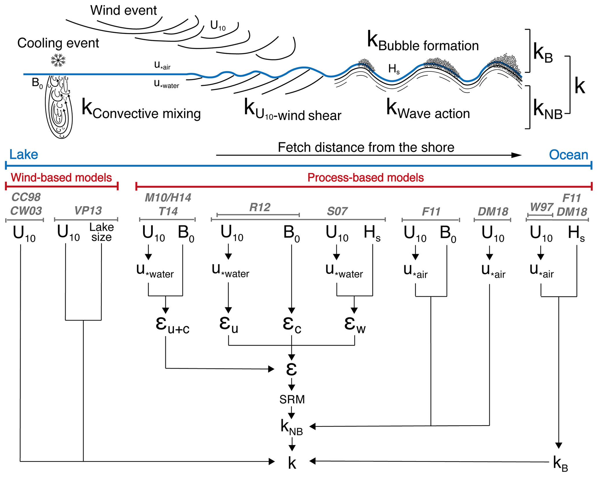
Figure 1 Conceptual scheme of the four main processes driving gas transfer velocity (k) in a large lake induced by wind and cooling events. These four processes are split into two types of k: k-bubble for the bubble formation (k_B=k_b) and k-no bubble for the convective mixing, wind shear, and wave action term which are added ($k_{\text{NB}}=k_{\mathrm{c}}+k_{\mathrm{u}}+k_{\mathrm{w}}$). Below this scheme, a non-exhaustive review of the conceptual approaches of k models used in first Fickian law is given. From left to right, the increase in the complexity level of k models and their study site (limnological to oceanic case) is visible. All of these variables are described in Sect. 2.4 and Table 1.

Table 1 Summary of the characteristics of k_Sc models for predicting the air–water gas transfer velocity based on wind speed (CC98 and CW03) and lake size (VP13), surface renewal model (T14, R12, and S07), COARSE approach (DM18), and both adapted models, namely SD21 and SD21-fit, from a combination of S07 and DM18.

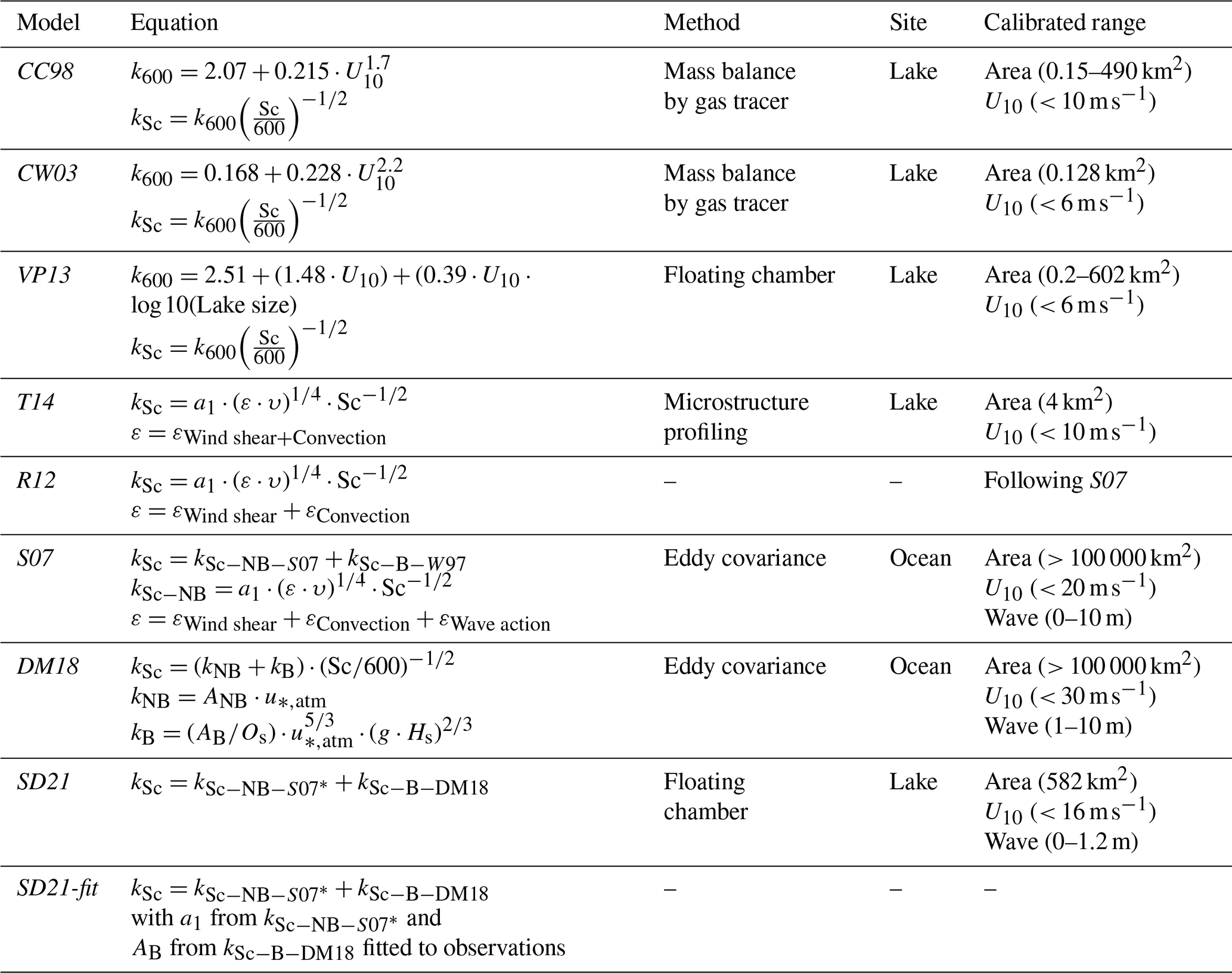
^∗ Adaptation of ε_{Wave action} for a large lake: CC98 – Cole and Caraco (1998), CW03 – Crusius and Wanninkhof (2003), VP13 – Vachon and Prairie (2013), T14 – Tedford et al. (2014), R12 – Read et al. (2012), S07 – Soloviev et al. (2007), and DM18 – Deike and Melville (2018).

k is inherently tied to turbulent mixing within the surface boundary layer, which enhances the diffusive gas exchange by renewing the surface mass content (Zappa et al., 2007). At the lake–atmosphere interface, turbulent mixing is the product of wind shear (k_u), buoyancy flux (k_c), and wind-driven surface waves, whose effect can be split into wave action (k_w) and wave breaking (k_b or k_B), with the latter producing air bubble and water spray (Fig. 1; Wüest and Lorke, 2003, Soloviev et al., 2007). Regarding the prominent role of wind action on surface turbulence, first quantitative models have empirically scaled k to wind speed (referenced at a 10 m height; U₁₀), as a proxy for the level of wind-driven turbulence (Fig. 1; Cole and Caraco, 1998; Crusius and Wanninkhof, 2003). The parameterisations of the k–wind relationships vary between authors (e.g. Klaus and Vachon 2020), as a likely consequence of the local characteristics of the lakes used in the calibration datasets (Table 1). However, all studies suggested a polynomial relationship between U₁₀ and k with an exponent larger than 1. Further development of empirical models integrated the lake surface area as a second parameter in the k–wind relationships, to account for the role of the fetch length for wind action (Vachon and Prairie, 2013). Generally, empirical wind-based models tend to underestimate fluxes, especially at low wind speed (e.g. Schubert et al., 2012; Heiskanen et al., 2014; Mammarella et al., 2015) where turbulent mixing through buoyancy flux is expected to take over wind shear. Moreover, these empirical models require a proper calibration each time they are applied in a new system with different characteristics, i.e. a new set of lakes and/or meteorological conditions (Klaus and Vachon, 2020), thereby limiting their universal applicability.

In parallel to empirical wind-based models, process-based models attempt to link k directly to near-surface turbulence. The surface renewal model (SRM) is one of the first, and still most widely used, theories (Danckwerts 1951; Lamont and Scott, 1970) with k depending on the product of the turbulent kinetic energy dissipation rate (ε) and the kinematic viscosity of water (υ), both to a power of one-quarter as follows:

$$\begin{array}{}\text{(2)}& k=a_{\mathrm{1}}(\mathit{\epsilon }\mathit{\upsilon }{)}^{\mathrm{1}/\mathrm{4}}{\text{Sc}}^{-\mathrm{1}/\mathrm{2}},\end{array}$$

where a₁ is a calibration constant parameter, and Sc is the Schmidt number. Recently, Lorke and Peeters (2006) and Katul and Liu (2017) demonstrated that this relationship, to which different approaches converge, can be seen as a universal scaling. As opposed to the practical empirical models presented above, process-based models have the potential to predict k using the turbulent dissipation rate over a wide range of environmental conditions extending beyond those encountered in the calibration dataset (Zappa et al., 2007). As for lakes, SRM k models have so far considered the friction velocity at the water side (u_*, wat) and the turbulence created by thermal convection using the buoyancy flux at the surface (B₀) (Fig. 1; Eugster et al., 2003; MacIntyre et al., 2010; Read et al., 2012; Tedford et al., 2014; Heiskanen et al., 2014). It is noteworthy that the SRM approach leads to k being related to u_*, wat (or U₁₀) to the first order (Wanninkhof, 1992; Lorke and Peeters 2006; see Sect. 2), whereas the empirical models described above predict a higher-order polynomial relationship. This inconsistency is tentatively solved in oceanography by adding another source of gas exchange associated with wind-waves' whitecaps. Early gas flux parameterisation already accounted for wind and buoyancy-driven turbulence as well as surface waves (Fig. 1; Woolf et al., 1997; Soloviev et al., 2007; Fairall et al., 2011). However, the buoyancy-driven contribution can often be neglected in oceanography, and recent efforts have been dedicated to a better parameterisation of the bubble enhancement term (Fig. 1; Deike and Melville, 2018). In lakes, wind fetch can be long enough to generate surface waves (Wanninkhof, 1992; Frost and Upstill-Goddard, 2002; Borges et al., 2004; Guérin et al., 2007), implying that surface waves could be a significant driver of k and subsequent CO₂ fluxes (Schilder et al., 2013; Vachon and Prairie, 2013). Thus, the role of surface waves has been essentially empirically accounted for in lake k models, through the polynomial scaling to U₁₀ in wind-based models, and most often neglected in studies using process-based parameterisations (mainly SRM) (e.g. Read et al., 2012). While this approximation may be appropriate for small-shielded lakes, it is likely to be insufficient in larger, long-fetched lakes.

Herein, we aim to identify the most adequate k model for Lake Geneva, a large, clear, hard-water lake in the Swiss Alps, to assess k values over a full annual cycle. We compare the performances of different models of gas transfer velocity, in their original or slightly modified published formulations from the limnological and oceanic literature. This set of models includes different levels of complexity, ranging from empirical models integrating wind speed and lake size to process-based models including wind shear, convection, and surface waves. Continuous ΔpCO₂ measurements by in situ automated sensors and CO₂ fluxes, obtained from a new generation of automated (forced diffusion) flux chamber, were collected during specific periods of intensive field survey covering a wide range of natural conditions. Empirical k values computed from chamber data are then compared to outputs from the different k models. Owing to the size of Lake Geneva, we anticipate that models accounting, implicitly or explicitly, for the four key exchange drivers (i.e. wind shear, convective mixing, wave action, and bubble formation) will show the highest accuracy and precision in their estimation of k and that a precise integration of surface wave effects in such a large system should enhance model predictions. Thereafter, the relative distribution of these components is computed over a full year and analysed in the scope of the temporal variability of the gas transfer velocity. Finally, we expect that extreme wind and associated wave events should contribute disproportionately to accumulated k values over the year. In such a case, episodic weather events could generate large CO₂ fluxes over very short timescales that should be accounted for when computing annual CO₂ emission budgets.

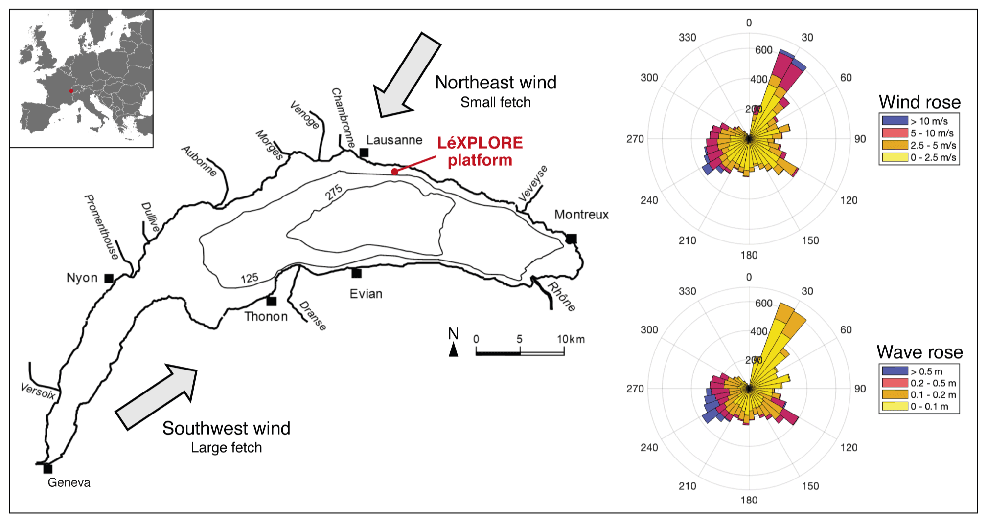
Figure 2 Location and map of Lake Geneva with the two prevailing winds (left) also depicted by the wind rose (top right). The wave rose highlights the highest wave field generated at the sampling location by the southwest wind with a larger fetch (bottom right). Both the wind and wave roses are computed with annual data from 13 June 2019 to 12 June 2020 at LéXPLORE.

2 Material and methods

2.1 Study site

Lake Geneva is a peri-Alpine lake defining part of the Swiss–French border, at 372 $\mathrm{m}\mathrm{a}.\mathrm{s}.\mathrm{l}.$ (metres above sea level) (46^∘26^′ N, 6^∘33^′ E). Its surface area (582 km²) and its maximum depth (309 m) make it the largest freshwater body in western Europe, with a volume of 89 km³ (Fig. 2). Lake Geneva is monomictic. The two prevailing winds are almost diametrically opposed and come from the southwest and northeast respectively (Fig. 2). The lake water has been surveyed monthly or fortnightly since the late 1950s (OLA-IS, AnaEE-France, INRAE of Thonon-les-Bains, and CIPEL; Rimet et al., 2020). The surface CO₂ concentrations, as computed from the routine temperature, alkalinity, and pH measurements (Stumm and Morgan, 1981), show a typical seasonal cycle with high, supersaturated values during winter mixing and values below saturation in summer (Perga et al., 2016).

2.2 Field data at LéXPLORE

All field data were collected from the LéXPLORE platform, a 10 m by 10 m pontoon equipped with high-tech instrumentation and installed on Lake Geneva in 2019 (Wüest et al., 2021). LéXPLORE is moored at a 110 m depth, 570 m off the northern lake shore (Fig. 2).

On LéXPLORE, local weather conditions (air temperature, wind speed and direction, relative humidity, short-wave radiation, and atmospheric pressure) were continuously recorded (at 10 min intervals) by a Campbell Scientific automatic weather station. Lake surface temperature was measured every minute at 50 cm depth using a Minilog II-T (VEMCO, resolution 0.01 ^∘C). The partial pressure of water surface CO₂ (pCO₂) was also measured at 50 cm depth during specific surveys (see Sect. 2.3) using a mini CO₂ sensor (Pro-Oceanus Systems Inc.) with an accuracy of ± 30 ppm. Values of pCO₂ in parts per million (ppm) were converted into micro-atmospheres (µatm) following the basic equation correcting for altitude (Russell and Denn, 1972). Therefore, we assume that the concentration and the temperature are homogeneous over the first 50 cm.

Fetch distance (m) from LéXPLORE to the lake shores considering wind direction was computed using data from the Federal Office of Topography online portal (Swisstopo geoportal: https://www.geo.admin.ch/, last access: 14 October 2020). The position of LéXPLORE is particularly relevant for this study as the fetch ranges from ∼ 0.5 to ∼ 30 km for the two prevailing winds. Significant wave height, H_s (in m), was computed after Hasselmann et al. (1973) according to the following equation:

$$\begin{array}{}\text{(3)}& H_{\mathrm{s}}=\mathrm{1.6}\times {\mathrm{10}}^{-\mathrm{3}}\cdot U_{\mathrm{10}}\cdot (\text{Fetch}/g{)}^{\mathrm{1}/\mathrm{2}},\end{array}$$

where g is the gravitational constant. This variable H_s is defined as the average height of the highest one-third of the waves (crest to trough) corresponding to the thickness over which the wind can push laterally (Wüest and Lorke, 2003). This equation is equivalent to the formulation by Carter (1982) that is more widely used in the oceanic literature. Simon (1997) tested the model for significant wave heights in Lake Neuchâtel (a lake close to Lake Geneva) with a fetch distance of 9 km. These results showed that the significant wave height in this lake was consistent with this oceanic formulation. However, Simon (1997) highlighted that the Joint North Sea Wave Project (JONSWAP) wave breaking parameterisation did not hold for winds greater than 5 m s⁻¹, producing faster wave breaking and with a higher probability in the case of surface waves that were not fully developed. Such lake waves are characterised by steeper slopes that favour their wave breaking and wave action (Wüest and Lorke, 2003).

The net CO₂ flux at the lake–atmosphere interface, F, was directly measured with an automated (forced diffusion) floating CO₂ flux chamber (eosFD, Eosense: environmental gas monitoring; Fig. A1; Risk et al., 2011), which was originally developed for soil flux studies. The flux chamber had a detection limit close to 0.05 $\mathrm{\mu }\mathrm{mol}{\mathrm{cm}}^{-\mathrm{2}}{\mathrm{h}}^{-\mathrm{1}}$ and measured F every 15 min in summer and 30 min in winter for battery-saving purposes. The standard floating chambers require quiet surface conditions (e.g. Cole et al., 2010; Vachon et al., 2010; Bastviken et al., 2015), thereby limiting studies to low to moderate wind speed conditions. One typical problem with floating chambers arises from the possible atmospheric leakage under rough surface conditions (Fig. A2a). To work around this problem, Vachon et al. (2010) recommend the creation of 10 cm long-edges entering the water (Fig. A2b), and this design also reduces artificial turbulence generated by the chamber's walls at surface. A second typical issue with this method is potential flux enhancement by artificial (chamber-generated) turbulence. This was also studied by Vachon et al. (2010), who demonstrated that the overestimations due to this effect can be as high as 1000 % at low wind but less than 50 % when the wind speed exceeds 4 m s⁻¹ in large lakes. At even higher wind speed, this overestimation should decrease further because the surface water turbulence becomes much greater than that produced by the floating chamber. Thus, our flux chamber was specifically conceived to increase stability under calm and windy conditions and to limit artificial turbulence, but we do not exclude a bias under low and moderate wind conditions (Figs. A1, A2c).

Regarding the operation of the eosFD, it has two independent cavities: one for the chamber and one for the atmosphere (Fig. A1). These are connected to the same CO₂ sensor by a pump which sends either the chamber gas or the air gas to the sensor at regular intervals (about 20 s) and then completely flushes the chamber cavity according to the programmed measurement time step (15 or 30 min). Therefore, the advantage of this new instrument is to have a constant monitoring of the chamber's variation but also of the atmosphere. In addition, the use of the same CO₂ sensor for the two measurements limits the need for intercalibration between CO₂ sensors. We tested the performance of the floating chamber by comparing the standard deviation of the CO₂ concentrations of the atmosphere and in the chamber estimated from two separated cavities (Fig. A1; Risk et al., 2011). We did not observe any difference in the standard deviation between high and low wind conditions (Fig. A3), suggesting that the measured fluxes remained reliable at high wind speed without leakage of the chamber.

We assessed the performances of our flux chamber during five specific periods over the annual cycle: 13–14 June 2019, 27–28 August 2019, 1–5 October 2019, 18–20 December 2019, and 20–26 February 2020. To select the most robust dataset for comparison with k estimates derived from models, we discarded flux data that were below the detection limit as well as CO₂ gradients that ranged within the uncertainty of sensors (i.e. ± 20 ppm for air and ± 30 ppm for water, resulting in a ± 50 ppm uncertainty) (Fig. A2). Accordingly, we were able to retain the most robust data points during the following deployment periods: 18–20 December 2019 and 20–26 February 2020. Finally, all these field data were standardised at a 1 h time step.

2.3 Computed k values from field data

k values (cm h⁻¹) from field observations (k_obs) were computed from the gas transfer velocity equation:

$$\begin{array}{}\text{(4)}& k_{\text{obs}}=F/(\mathit{\alpha }\cdot \mathrm{\Delta }\mathit{\text{p}}{\mathrm{CO}}_{\mathrm{2}}),\end{array}$$

where F is the measured CO₂ flux ($\mathrm{\mu }\mathrm{mol}{\mathrm{cm}}^{-\mathrm{2}}{\mathrm{h}}^{-\mathrm{1}}$); α is the gas solubility coefficient ($\mathrm{\mu }\mathrm{mol}{\mathrm{cm}}^{-\mathrm{3}}\mathrm{\mu }{\mathrm{atm}}^{-\mathrm{1}}$), which depends on the measured water temperature (Wanninkhof, 1992); and ΔpCO₂ is the differential of pCO₂ measured at 0.5 m below the surface (pCO_2-water) and pCO₂ at saturation (pCO_2-sat; in ppm) measured from the flux chamber corrected by altitude (µatm). It is noteworthy that the chemical enhancement factor (Wanninkhof and Knox, 1996) was not considered in this equation, as the fluxes retained corresponded to conditions of moderate pH (i.e. < 8). k_obs was then standardised in k₆₀₀ using the dimensionless Schmidt number (Sc) of CO₂: $k_{\mathrm{600}-\text{obs}}=k_{\text{obs}}\cdot (\mathrm{600}/\text{Sc}{)}^{-\mathrm{1}/\mathrm{2}}$ (600 for freshwater standardised at 20 ^∘C).

2.4 Models for air–water gas transfer velocity

After years of debate, a consensus has begun to emerge on the relationship linking k, the intensity of turbulence, and Sc (Eq. 2), even when starting from different physical assumptions (see Katul et al., 2018). In this study, we selected six parameterisations widely used in limnology and oceanography, combining specific calibration characteristics (Table 1). We first show that they can all be expressed following Eq. (2) for wind shear and convection, despite their different formulations. We then develop the effects of surface waves from oceanic models and adapt the wave action for a large lake. The final lake model integrating the wave effect is ultimately calibrated using our field data (Table 1).

2.4.1 Wind shear stress

We start with the case where near-surface dynamics are driven by a weak to moderate wind, in the absence of heat exchange. In this case, the contribution of surface waves can be neglected and the wind stress (${\mathit{\tau }}_{\mathrm{0}}={\mathit{\rho }}_{\text{air}}\cdot C_{\mathrm{10}}\cdot U_{\mathrm{10}}^{\mathrm{2}}$, where ρ_air is air density and C₁₀ is the drag coefficient at 10 m) is equal to the tangential shear stress (${\mathit{\tau }}_{\mathrm{t}}={\mathit{\rho }}_{\text{wat}}\cdot {u_{\ast ,\text{wat}}}^{\mathrm{2}}$, where ρ_wat is water density). The relationship between ε and the sheared velocity on the water side, $u_{\ast ,\text{wat}}$, is then derived from a law-of-the-wall scaling for the velocity profile: $\mathit{\epsilon }=u_{\ast ,\text{wat}}^{\mathrm{3}}/\mathit{\kappa }z\left(\mathrm{0}\right)$, where κ is the von Kármán constant (= 0.41), and z(0) is the thickness of the diffusive boundary layer. This relationship leads to

$$\begin{array}{}\text{(5)}& k_{\text{NB}}=a_{\mathrm{1}}\cdot {\left(\mathit{\nu }{u}_{\ast ,\text{wat}}^{\mathrm{3}}/\mathit{\kappa }z\left(\mathrm{0}\right)\right)}^{\mathrm{1}/\mathrm{4}}{\text{Sc}}^{-\mathrm{1}/\mathrm{2}}.\end{array}$$

The challenge is then to define z(0). Tedford et al. (2014) followed an ad hoc observational approach and chose z(0) = 0.15 m as the shallower depth where ε was measured. In contrast, theoretical studies have linked z(0) to the thickness of the diffusive or viscous sublayer (∼ 0.1–1 cm). In line with theory, we scale this layer as $z\left(\mathrm{0}\right)=c\mathit{\nu }/u_{\ast ,\text{wat}}$ (Wüest and Lorke, 2003; Lorke and Peeters, 2006) with c as a constant value. Taking c = 114 (Soloviev et al., 2007), the thickness of this layer typically ranges from 0.04 to 0.14 m under a wind regime of 10 to 1 m s⁻¹. Therefore, we modify Eq. (5) to compute the interfacial (no bubble, NB) exchange coefficient:

$$\begin{array}{}\text{(6a)}& k_{\text{NB}}=a_{\mathrm{1}}{u}_{\ast ,\text{wat}}(\mathrm{1}/\mathit{\kappa }c{)}^{\mathrm{1}/\mathrm{4}}{\text{Sc}}^{-\mathrm{1}/\mathrm{2}},\end{array}$$

or

$$\begin{array}{}\text{(6b)}& k_{\text{NB}}=a_{\mathrm{1}}({\mathit{\rho }}_{\text{air}}/{\mathit{\rho }}_{\text{wat}})C_{\mathrm{10}}{U}_{\mathrm{10}}(\mathrm{1}/\mathit{\kappa }c{)}^{\mathrm{1}/\mathrm{4}}{\text{Sc}}^{-\mathrm{1}/\mathrm{2}}.\end{array}$$

These equations show that the SRM formulation (Table 1, Fig. B1; Soloviev et al., 2007; Read et al., 2012) is analogous to the Coupled Ocean–Atmosphere Response Experiment Gas transfer algorithm (COAREG) flux (Fairall et al., 2011) and to the formulation used in Deike and Melville (2018) with the sheared velocity on the atmosphere side, $u_{\ast ,\text{atm}}$ (Table 1: DM18). Indeed, when equating the expression by Deike and Melville (2018),

$$\begin{array}{}\text{(7)}& \begin{array}{rl}{k}_{\text{NB}}& =A_{\text{NB}}{u}_{\ast ,\text{atm}}(\text{Sc}/\mathrm{600}{)}^{-\mathrm{1}/\mathrm{2}}\\ & =A_{\text{NB}}{u}_{\ast ,\text{wat}}({\mathit{\rho }}_{\text{wat}}/{\mathit{\rho }}_{\text{atm}}{)}^{\mathrm{1}/\mathrm{2}}(\text{Sc}/\mathrm{600}{)}^{-\mathrm{1}/\mathrm{2}}.\end{array}\end{array}$$

With Eq. (6a), we find that the coefficient a₁ = 0.29 in Soloviev et al. (2007) and Read et al. (2012) is essentially equivalent to the coefficient A_NB = $a_{\mathrm{1}}\left(\mathit{\kappa }c{)}^{-\mathrm{1}/\mathrm{4}}\right(\mathrm{1}/\mathrm{600}{)}^{\mathrm{1}/\mathrm{2}}({\mathit{\rho }}_{\text{wat}}/{\mathit{\rho }}_{\text{air}}{)}^{-\mathrm{1}/\mathrm{2}}\approx \mathrm{1.5}\times {\mathrm{10}}^{-\mathrm{4}}$ in Deike and Melville (2018) (Fig. B1), which, in turn, was found to be equal to the coefficient of A = 1.5 in Fairall et al. (2011). These results agree with Lorke and Peeters (2006), who derived a unified relation for interfacial fluxes (air–water and water–sediment) through a linear relationship of u_*, wat with k, especially at the bottom interface where shear is the only relevant process. Furthermore, Eq. (6) has a similar (i.e. quasi-linear) k–wind relationship to the data-driven parameterisation from VP13 but cannot explain the higher-order polynomial relationship reported in CW03 and CC98.

2.4.2 Convection

A second source of dissipation at the surface is the convection (ε_c) resulting from surface cooling. In the SRM formulation, only the negative buoyancy flux is considered when this term directly enters into the turbulent kinetic equation as a production term. The combination of wind shear and free convection near a boundary is described by the Monin–Obukhov similarity theory (MOST) with a general form derived from a turbulent kinetic energy balance (Lombardo and Gregg, 1989; Tedford et al. 2014):

$$\begin{array}{}\text{(8)}& \mathit{\epsilon }\left(z\right)={\mathit{\epsilon }}_{\mathrm{u}}\left(z\right)\left(c_{\mathrm{u}}+c_{\mathrm{c}}⌊{\displaystyle \frac{z}{L_{\text{MO}}}}⌋\right),\end{array}$$

where L_MO is the Monin–Obukhov length scale defined as $L_{\text{MO}}=u_{\text{*,\hspace{0.17em}wat}}^{\mathrm{3}}/\mathit{\kappa }{B}_{\mathrm{0}}$, including $\mathit{\epsilon }\left(z\right)=c_{\mathrm{u}}\cdot {\mathit{\epsilon }}_{\mathrm{u}}+c_{\mathrm{c}}\cdot {\mathit{\epsilon }}_{\mathrm{c}}$ in Eq. (2). The latter expression can be rearranged as follows:

$$\begin{array}{}\text{(9)}& k_{\text{NB}}=a_{\mathrm{1}}\left({\mathit{\epsilon }}_{\mathrm{u}}(c_{\mathrm{u}}+c_{\mathrm{c}}\cdot B_{\mathrm{0}}/{\mathit{\epsilon }}_{\mathrm{u}}{)}^{\mathrm{1}/\mathrm{4}}\right){\text{Sc}}^{-\mathrm{1}/\mathrm{2}},\end{array}$$

where a₁ ranges in the literature from 0.2 to 1.2 (Soloviev et al., 2007; MacIntyre et al., 2010; Tedford et al., 2014; Heiskanen et al. 2014; Winslow et al., 2016), c_u ranges from 0.84 to 1 (Winslow et al., 2016), and c_c ranges from 0.37 to 2.5 (Wyngaard and Coté, 1971; Tedford et al., 2014). Hereafter, we use the following set of values: c_u = 1 and c_c = 1. Fairall et al. (2011) used an essentially equivalent approach but formulated in terms of a Richardson number to describe the partitioning between dissipation from convection and wind shear, expressing the wind shear in terms of the air-side friction velocity: $R_{\mathrm{f}}=B_{\mathrm{0}}\mathit{\upsilon }/u_{\text{*,\hspace{0.17em}atm}}^{\mathrm{4}}$, which can be integrated into Eq. (9) as

$$\begin{array}{}\text{(10)}& k_{\text{NB}}=a_{\mathrm{1}}{\left({\displaystyle \frac{{\mathit{\rho }}_{\text{atm}}}{{\mathit{\rho }}_{\text{wat}}}}\right)}^{\mathrm{1}/\mathrm{2}}{u}_{\text{*,\hspace{0.17em}atm}}{\left({\displaystyle \frac{c_{\mathrm{u}}}{\mathit{\kappa }c}}\left(\mathrm{1}+{\displaystyle \frac{R_{\mathrm{f}}}{R_{\mathrm{f},\mathrm{c}}}}\right)\right)}^{\mathrm{1}/\mathrm{4}}{\left({\displaystyle \frac{\text{Sc}}{\mathrm{600}}}\right)}^{-\mathrm{1}/\mathrm{2}},\end{array}$$

where $R_{\mathrm{f},\mathrm{c}}=\frac{c_{\mathrm{u}}{\mathit{\rho }}_{\text{atm}}^{\mathrm{2}}}{c_{\mathrm{c}}{\mathit{\rho }}_{\text{wat}}^{\mathrm{2}}\mathit{\kappa }c}$. The details of this demonstration can be seen in Soloviev and Schlüssel (1994).

2.4.3 Wave action

The effect of surface waves is commonly implemented in oceanography but barely considered in limnology. All process-based models rely on the same parameterisation of energy dissipation by wind shear and convection. However, they differ in how they parameterise energy dissipation by wave action and wave breaking.

The contribution of the wave action (ε_w) is, accordingly, added as a third source of turbulence (Fig. 1). In the presence of surface waves, the balance between τ_t and τ₀ no longer holds. Therefore, Soloviev and Schlüssel (1994) added a corrective factor, φ, using the Keulegan number ($\text{Ke}=u_{\text{*,\hspace{0.17em}wat}}^{\mathrm{3}}/\left(g\mathit{\nu }\right))$, in order to decrease the component ${\mathit{\tau }}_{\mathrm{t}}={\mathit{\tau }}_{\mathrm{0}}\cdot \mathit{\phi }$ (where $\mathit{\phi }=\mathrm{1}/(\mathrm{1}+\text{Ke}/{\text{Ke}}_{\mathrm{c}})$), with the critical Keulegan number (Ke_c) defined in Soloviev and Lukas (2006). As a result, the equation for shear-driven dissipation ε_u(z) is as follows:

$$\begin{array}{}\text{(11)}& {\mathit{\epsilon }}_{\mathrm{u}}\left(z\right)={\displaystyle \frac{u_{\text{*,\hspace{0.17em}wat}}^{\mathrm{4}}}{\mathit{\kappa }c\mathit{\upsilon }}}\cdot {\mathit{\phi }}^{\mathrm{2}}.\end{array}$$

Following this step, the turbulent kinetic energy dissipation rate from wave action (ε_w) is added and defined with the Keulegan number by Soloviev et al. (2007) as follows:

$$\begin{array}{}\text{(12)}& \begin{array}{rl}{\mathit{\epsilon }}_{\mathrm{w}}=& {\mathit{\alpha }}_W{\left({\displaystyle \frac{\mathrm{3}}{B{S}_q}}\right)}^{\mathrm{1}/\mathrm{2}}\\ & \cdot {\displaystyle \frac{(\text{Ke}/{\text{Ke}}_{\text{c}}{)}^{\mathrm{3}/\mathrm{2}}}{(\mathrm{1}+\text{Ke}/{\text{Ke}}_{\text{c}}{)}^{\mathrm{3}/\mathrm{2}}}}{\displaystyle \frac{u_{\text{*,\hspace{0.17em}wat}}g}{\mathrm{0.062}\mathit{\kappa }{C}_{\mathrm{T}}(\mathrm{2}\mathit{\pi }{A}_{\mathrm{w}}{)}^{\mathrm{3}/\mathrm{2}}}}{\displaystyle \frac{{\mathit{\rho }}_{\text{atm}}}{{\mathit{\rho }}_{\text{wat}}}},\end{array}\end{array}$$

where $C_{\mathrm{T}}=(z_{\mathrm{0}}/H_{\mathrm{s}})$. z₀ is the surface roughness scale from the water side, and the C_T value is set as a constant at 0.6 (more details are given in Soloviev et al., 2007). This definition does not hold for closed basins because, in the case of incompletely developed waves, the dissipation of energy from wind shear transmitted to the waves is not fully redistributed in the water body (Simon, 1997). Hence, for the application in Lake Geneva, we followed Terray et al. (1996), who defined a varying C_T:

$$\begin{array}{}\text{(13)}& C_{\mathrm{T}}=\mathrm{1.38}\times {\mathrm{10}}^{-\mathrm{4}}{\left({\displaystyle \frac{U_{\mathrm{10}}}{C_{\mathrm{p}}}}\right)}^{\mathrm{2.66}},\end{array}$$

where C_p is the peak speed of the wave spectrum defined in Deike and Melville (2018) according to Toba (1972, 1978). This leads to C_T ≪ 1. This allows one to increase the effect of ε_w (inversely proportional to C_T in Eq. 12) on k. Here, we used this formulation to adapt the S07 ocean model for a large lake (closed basin). Henceforth we refer to the adapted uncalibrated and calibrated models as SD21 and SD21-fit respectively (Table 1). Finally, these three terms of ε (ε_u, ε_c, and ε_w) can be added before computing the SRM (Eq. 2) for determining k-no bubble (k_NB).

2.4.4 Bubble enhancement

Additional deviations from the linear relationship to U₁₀ are explained by the gas transfer resulting from bubbles and sprays during wave breaking. This mechanism is accounted for by adding a k-bubble (k_B) term to the previously mentioned k_NB. Soloviev et al. (2007) used the empirical k-bubble parameterisation from Woolf et al. (1997):

$$\begin{array}{}\text{(14)}& k_{\mathrm{B}}=W{\displaystyle \frac{\mathrm{2450}}{O_{\mathrm{s}}{\left(\mathrm{1}+\frac{\mathrm{1}}{{\left(\mathrm{14}{O}_{\mathrm{s}}{\text{Sc}}^{-\mathrm{0.5}}\right)}^{\mathrm{1}/\mathrm{1.2}}}\right)}^{\mathrm{1}/\mathrm{2}}}},\end{array}$$

where W is the fractional whitecap coverage only expressed as a function of wind ($\mathrm{3.84}\times {\mathrm{10}}^{-\mathrm{6}}\cdot U_{\mathrm{10}}^{\mathrm{3.41}}$), and O_s is the Ostwald gas solubility. This formulation does not take wave height into account (Fig. B1). Nevertheless, a recent study (Deike and Melville, 2018) performed a new numerical process-based parameterisation for gas transfer velocity from bubble enhancement considering H_s through the following equation:

$$\begin{array}{}\text{(15)}& k_{\mathrm{B}}={\displaystyle \frac{A_{\mathrm{B}}}{O_{\mathrm{s}}}}{u}_{\ast ,\text{atm}}^{\mathrm{5}/\mathrm{3}}(g{H}_{\mathrm{s}}{)}^{\mathrm{2}/\mathrm{3}}{\left({\displaystyle \frac{\text{Sc}}{\mathrm{600}}}\right)}^{-\mathrm{1}/\mathrm{2}},\end{array}$$

where A_B is an empirical factor with dimension (= 10⁻⁵ m⁻² s²), and O_s is defined by the ideal gas constant (R), the surface water temperature (T₀), and the CO₂ solubility coefficient in freshwater (α) (Reichl and Deike, 2020). The gas transfer velocity is the expressed as a sum of the no bubble k_NB and bubble k_B components (Table 1: S07, DM18, SD21, and SD21-fit) following Keeling (1993) and Woolf et al. (1997, 2005). Our adapted model for lake includes a refined parameterisation of the wave action term ε_w from S07 along with the bubble term from DM18. For these reasons, the model will be called SD21 in the rest of the paper. In addition, for the appellation SD21-fit, the a₁ parameter of Eq. (2) and the A_B parameter of Eq. (15) were fitted to the k₆₀₀ observations (a₁ = 0.33 and A_B = 3 × 10⁻⁵ m⁻² s²).

With this review of existing and adapting parameterisations, we show that (i) there is a discrepancy between an SRM-based model with shear stress as the only energy source and empirical parameterisations with a polynomial (order > 1) wind-based relationship. Such a discrepancy is tentatively resolved by adding the effect of convection and surface waves. (ii) We further highlight that most fitting parameters from the different SRM-based models are in good agreement. (iii) We finally recall that it is possible to provide a unifying parameterisation of k with an SRM model including wind shear, wind-induced waves, and convection with only a few input parameters such as U₁₀, B₀, and Fetch.

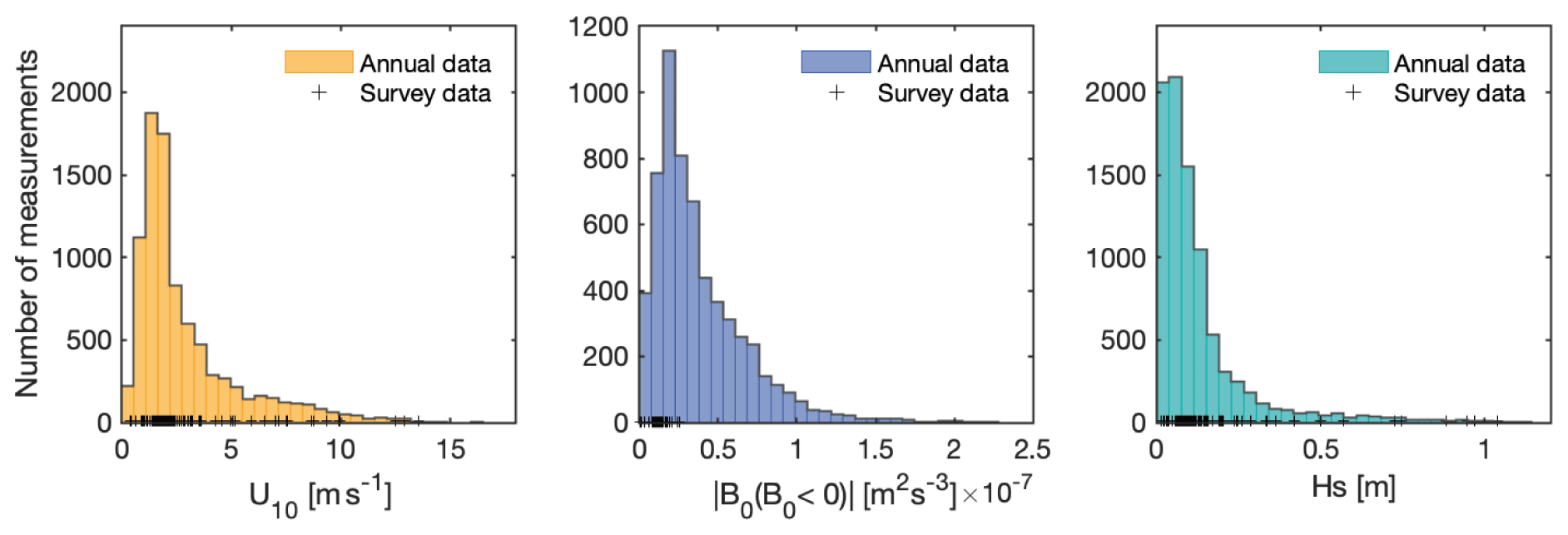
Figure 3 The annual distribution of the three main components used to compute k₆₀₀ models: wind speed at 10 m (orange), buoyancy flux at the surface during cooling (blue), and significant wave height (turquoise). These survey data observed during CO₂ flux measurements after quality control (+) are also shown.

3 Results

3.1 Observed and predicted k

After quality check, our dataset contains 94 discrete CO₂ flux observations. We first assess the representativeness of our sampling by comparing the survey-specific and annual distributions of the three main inputs for k models: U₁₀ (all models), B₀ during convective periods (T14, S07, SD21, and SD21-fit), and H_s (S07, DM18, SD21, and SD21-fit) (Fig. 3; the temporal evolution of these three terms is shown in Fig. C1). From 13 June 2019 to 12 June 2020, the average wind speed over Lake Geneva is 2.9 m s⁻¹ with a mode at 2.5 m s⁻¹; very low wind speeds (< 1 m s⁻¹) are encountered 12 % of the year, whereas high (> 5 m s⁻¹) to very high (> 10 m s⁻¹) wind events represent 15 % and 2 % of the year respectively. The sampling surveys covered the full annual range of U₁₀. Average and modal values of B₀ over the year are close to 0.25 × 10⁻⁷ m² s⁻³. However, the sampling covered only the lowest 50 % of the annual distribution and undersampled conditions of potentially strong convection. Considering that the dissipation by buoyancy flux, as parameterised in the process-based models, is already well known in the literature and that it is not the central point of our study, we posit that the undersampling of B₀ is not expected to significantly affect our analysis. The predicted modal H_s value is 0.15 m over the year. Events of high H_s (> 0.4 m) represent 6 % of the year, with a maximum H_s of 1.1 m. As for U₁₀, the surveys covered the full range of annual H_s.

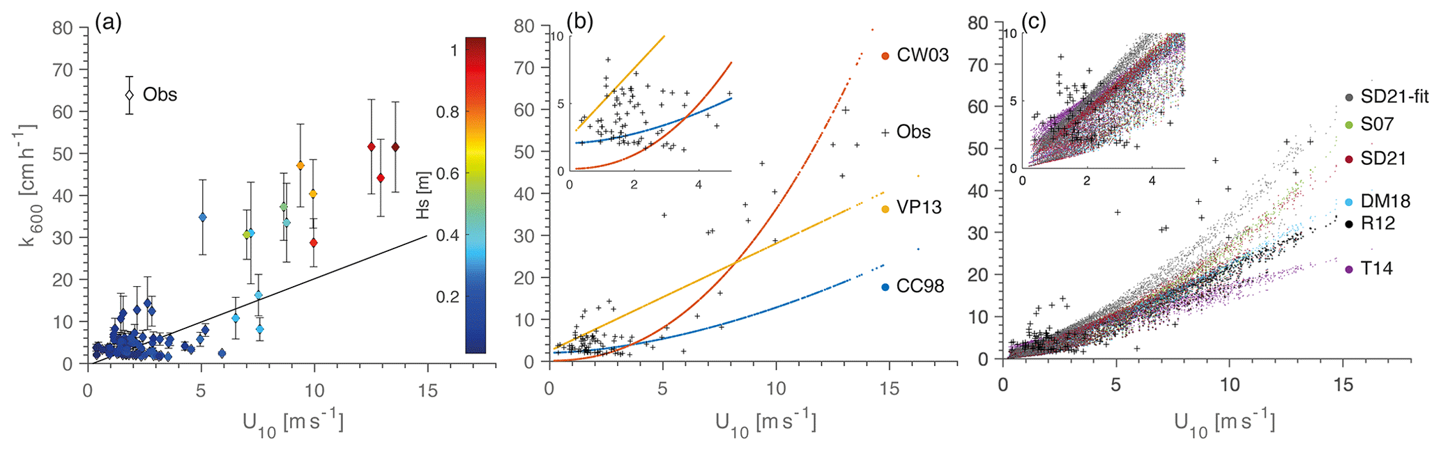
Figure 4 (a) k₆₀₀ observed as a function of U₁₀ and coloured according to H_s (colour bar), showing the error bars produced by the uncertainty of ΔCO₂ (± 50 ppm) as well as the $u_{\ast }-k_{\mathrm{600}}$ linear regression (solid line; see also Fig. B1); (b) k₆₀₀ wind-based models (CC98, CW03, and VP13); (c) k₆₀₀ process-based models (T14, S07, DM18, SD21, and SD21-fit) computed with annual data. Observed k₆₀₀ derived from CO₂ flux chamber measurements is shown using the “+” symbol.

Table 2 RMSE of k₆₀₀ models for all wind speed (U₁₀), U₁₀ < 5 m s⁻¹ (i.e. LW), and U₁₀≥ 5 m s⁻¹ (i.e. SW).

k₆₀₀ values based on observations are shown in Fig. 4a with their error bars corresponding to the uncertainties of the pCO₂ in air and in water (± 50 ppm). We notice that all of the measurements with a wave height > 0.4 m were observed for wind speeds > 5 m s⁻¹, and the corresponding k₆₀₀ values are located above the linear function (i.e. from a linear regression against wind shear velocity; Fig. B1) scaling k₆₀₀ to u_∗ (i.e. first-order relationship). We then compare the k₆₀₀ observed during the specific surveys to the values computed with all k₆₀₀ models throughout the annual cycle, in relation to U₁₀ (Fig. 4b, c). Table 2 provides the root-mean-square errors (RMSEs) for all model estimates compared to k_obs during the flux surveys, (i) for the full dataset (All Wind), and split (ii) for low wind (< 5 m s⁻¹, LW) and (iii) strong wind conditions (≥ 5 m s⁻¹, SW). The three empirical wind-based models only depend on wind (Fig. 4b). Both CC98 and CW03 were originally calibrated for small lakes, using a mass balance calibration method (Table 1). However, they lead to divergent gas transfer velocities, particularly above 5 m s⁻¹, illustrated by a RMSE for SW as high as 22.8 cm h⁻¹ for CC98, whereas CW03 performs better (RMSE SW = 12.8 cm h⁻¹). Furthermore, both models underestimate k₆₀₀ at low wind (Fig. 4a), with a higher deviation for CW03 (Table 2). The k values predicted by VP13 are closer to those of the process-based models that explicitly integrate wave actions (S07 and DM18) (Fig. 4b, c), demonstrating that lake size integration in the empirical model captures at least part of the wave action on k. Performances of VP13 at strong winds (RMSE SW = 12.7 cm h⁻¹) were better than those of the ocean-derived models integrating surface waves (RMSE SW = 13–15.9 cm h⁻¹). However, VP13 shows a positive offset during calm periods, along with the highest RMSE of the set of models at low wind speed (Fig. 4b, Table 2).

The process-based models (Fig. 4c) provide different k₆₀₀ values for a given wind speed, owing to the integration of additional environmental components (i.e. the varying drag coefficient, the convective mixing in R12 and T14, and the effect of waves in S07, DM18, SD21, and SD21-fit). All process-based models are similar at low winds, as they share a common physical basis for parameterisation of wind shear and convection. Therefore, they lead to similar RMSEs (2.9–3.5 cm h⁻¹) under such conditions, where surface waves are negligible (Table 2). Divergences occur at higher wind speeds. T14, initially developed for small lakes with limited wind exposure, performed the worst (RMSE = 19.8 cm h⁻¹). This increased k underestimation at high winds can be attributed to (i) dissipation by wave action and bubble formation not being considered (in R12 and T14) and (ii) to the use of a constant z(0) = 0.15 m in the T14 model (Eq. 5). This approximation of the diffusive layer is consistent with low wind speed but is almost 1 order of magnitude too large under strong wind speed. Other process-based models, designed for greater wind range (> 10 m s⁻¹), integrate surface waves and, as a result, lead to better estimates than R12 and T14 (RMSE = 10.4–15.9 cm h⁻¹). However, the ocean wave model of DM18 shows lower performances at strong winds than CW03 and VP13 (Fig. 4b, c). Finally, the specific fit parameterisation of the SD21-fit model improves the performance at high wind speeds by ∼ 30 % (RMSE = 10.5 cm h⁻¹), outperforming all the other methods.

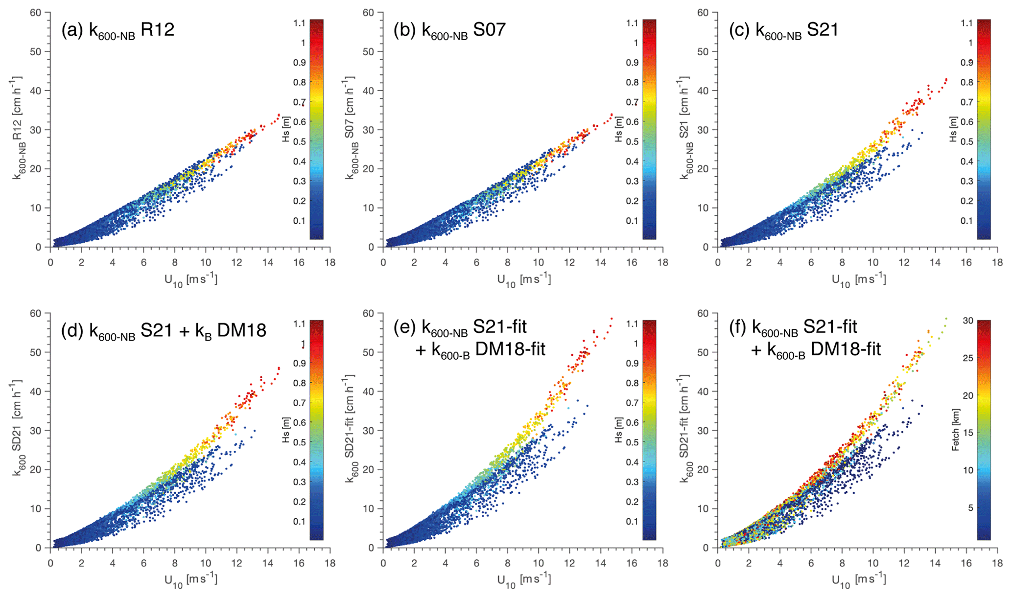
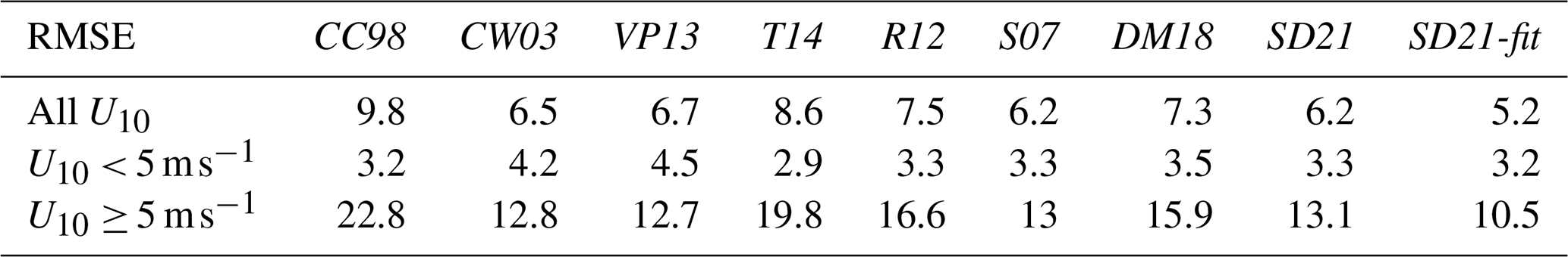
Figure 5 The U₁₀ vs. k₆₀₀ relationship modelled and coloured according to H_s (colour bar) in panels (a)–(e) as well as coloured according to fetch distance (colour bar) in panel (f): (a) R12 integrating wind shear and convection; (b) S07 integrating wind shear, convection, and wave action for fully developed waves; (c) S21 integrating wind shear, convection, and wave action for waves that are not fully developed; (d) SD21 is similar to S21 but the k-bubble term of DM18 is added; (e, f) SD21-fit is similar to SD21 but with a₁ and A_B fitted to observed k.

3.2 Surface wave integration

Herein, we scrutinise how those varying parameterisations ultimately alter the shape of relationship between k₆₀₀ and U₁₀. In R12 (Fig. 5a), wind is only included through wind shear, resulting in a linear relationship between k₆₀₀ and U₁₀, as already anticipated. Adding the wave action (no bubble) through the S07 parameterisation (Fig. 5b) does not lead to any significant departure from the minimal R12 model. Adapting wave action by decreasing C_T (for the no bubble term) leads to a departure from the wind shear linear relationship for H_s > 0.4 m (Fig. 5c).

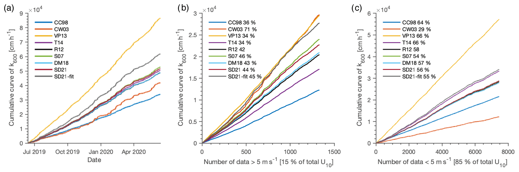
Figure 6 (a) Cumulative k₆₀₀ modelled over an annual cycle; (b) cumulative k₆₀₀ for wind > 5 m s⁻¹; (c) cumulative k₆₀₀ for wind ≤ 5 m s⁻¹.

Adding the k-bubble term related to wave breaking of DM18 further increases this deviation from the linear k₆₀₀–U₁₀ relationship but also scatters k₆₀₀ estimates for a given U₁₀ (Fig. 5d). Finally, the fitting with observationally based k₆₀₀ improves the estimation for strong wind (Fig. 5e, Table 2). Given the range of wind fetch from ∼ 0.5 to ∼ 30 km, the contribution of waves varies for a given wind speed depending on the fetch, as evidenced by the scattering of the parameterised k₆₀₀ for a given U₁₀ (Fig. 5f). A significant modification of k₆₀₀ by wave action and wave breaking occurs for a fetch length > 15 km and U₁₀ > 5 m s⁻¹ (Fig. 5f), in the case of Lake Geneva, generating wave of H_s > 0.4 m (Fig. 5e).

Compared with k₆₀₀ estimated by R12 (Fig. 5a), the SD21 and SD21-fit models provide k estimates that are 20 %–50 % higher for U₁₀ = 10 m s⁻¹ respectively and 40 %–70 % higher for U₁₀ = 15 m s⁻¹ respectively. Therefore, adapting the surface waves, through the change in the wave action for incompletely developed waves and the fitting to observed data encountered in local lake conditions, leads to better performances of the SD21 models. SD21-fit reached the lowest RMSE at all wind speeds and was thereafter used as a reference for the modelling of the annual gas transfer velocities.

3.3 Annual cumulative gas transfer velocity and the effect of extreme conditions

We show above that models accounting for surface waves better represent the non-linear increase in k₆₀₀ at high winds. Because high-wind events remain rare, we test whether a better representation of k₆₀₀ during rare, high-wind events affects the local estimates of k₆₀₀ over a full year. To this end, cumulative sums of hourly k₆₀₀ were computed over a full annual cycle (13 June 2019–12 June 2020) for all k models (Fig. 6). The annual dynamics, such as the annually averaged k₆₀₀, were compared using SD21-fit as a new reference model.

Cumulated k₆₀₀ computed for SD21-fit shows some episodic steep increases between December and March, due to the winterly prevalence of high-wind events (the winter average wind speed, 3.25 m s⁻¹, was greater than the summer mean, 2.55 m s⁻¹, by 25 %) and greater significant wave height (the winter average wave height, 0.15 m, was greater than the summer value, 0.10 m, by 50 %) (Fig. C1). The average hourly k₆₀₀ by the SD21-fit model is 7.3 ± 7.4 cm h⁻¹ (mean ± SE, Fig. 6a). Periods of high winds, although accounting for only 15 % of data points, contribute 44 % of annually cumulative k₆₀₀ in the SD21 and SD21-fit models (Fig. 6b), whereas periods of high waves (H_s≥ 0.4 m), accounting for only 6 % of data points, contribute to more than 20 % of annually cumulative k₆₀₀. The wind-based models are those for which cumulative k₆₀₀ diverges the most from the SD21-fit reference model, with the lowest annual averaged k₆₀₀ for CC98 and CW03 (3.9 ± 2.7 and 4.8 ± 9.3 respectively) and the highest for VP13 (9.9 ± 6.1). These divergences arise from the low performances of these models at low wind regimes (Figs. 4a, 6b; Table 2), which represent 85 % of annual data points. All of the other process-based models have relative dynamics of cumulative k₆₀₀ similar to that of the SD21-fit model and end up with annually averaged k₆₀₀ that are 15 % lower than for the SD21-fit. The representation of k₆₀₀ at low wind speeds is similar for all process-based models, and the divergence arises from the representation of the rarer high-wind-speed episodes, which contribute to 43 %–46 % of annual cumulative k₆₀₀ (Fig. 6b).

4 Discussion

The history of k models, simulating the gas transfer velocity for surface waters, dates back from the early 1990s. k models have been developed and tested in small lakes sheltered from winds (e.g. Crusius and Wanninkhof, 2003; Tedford et al., 2014), large lakes under low to moderate wind speed (Vachon and Prairie, 2013), and oceans (e.g. Soloviev et al., 2007; Fairall et al., 2011; Esters et al., 2017; Deike and Melville, 2018). While the effects of surface waves on k can be neglected in small lakes, we question whether this assumption holds for large lakes such as Lake Geneva, in which surface waves are frequently observed (Figs. 2, C1). We evaluated the performance of different experimental-based and process-based models to estimate k₆₀₀ in the large Lake Geneva. We show that integrating the effect of wave formation at high wind speeds and long fetch better represents the sharp increase in the k₆₀₀ values during such episodic windy events.

4.1 Choice of k models

Wind-based models have long been known to misestimate k₆₀₀ at low wind speeds (Eugster et al., 2003; MacIntyre et al., 2010; Erkkilä et al., 2018). Consistently, wind-based models showed the lowest performances for Lake Geneva, especially at low wind speeds (CW03 and VP13), which resulted in large discrepancies in annually averaged and cumulative k₆₀₀ over the full year. They are, however, easy to compute, require few inputs (only U₁₀), and remain by far the most used to estimate lakes' CO₂ emissions worldwide (e.g. Raymond et al. 2013). Another possibility is to broadly adopt process-based models. The presented process-based models require input data that are currently more easily accessible and are routinely acquired at high frequency in many lakes: wind speed, heat flux, and wind fetch (i.e. distance from the shore). The development of R packages, such as “LakeMetabolizer” (Winslow et al., 2016), in which the calculations of process-based models are implemented also alleviates their computational difficulty. Both increased data availability and computational tools should foster the use of process-based k models, which hold great potential to obtain more accurate global k₆₀₀ estimates.

The analysis of the models adapted from the existing literature to account for the effect of lake surface waves, SD21 and SD21-fit (Fig. 5d, e, f), showed that the wave contribution to k becomes significant for H_s > 0.4 m, corresponding, for Lake Geneva, to winds blowing at 5 m s⁻¹ from the southwest where the fetch length is maximal (> 15 km) with respect to the measurement site. A significant contribution to the gas transfer velocity by surface waves is expected in lakes where H_s > 0.4 m is not infrequent. Wave heights beyond this threshold value of H_s are frequently encountered in lakes that are larger than or a similar size to Lake Geneva (6 % of annual time at the LéXPLORE platform). In the Great Lakes of North America, Hubertz et al. (1991) showed that the mean wave heights of all of these lakes were > 0.4 m in summer and close to 1 m in winter with a maximum of up to 5 m. H_s > 0.4 m can also form over elongated lakes of smaller size, such as smaller Swiss lakes (e.g. Lake Neuchâtel and Lake Bienne) (Amini et al., 2017). As SD21-fit is a process-based model integrating the four main processes in a mathematically coherent way, we would expect that it can be applied to lakes experiencing H_s > 0.4 m and can improve the accuracy of k estimates. Because waves can physically damage inshore and offshore infrastructure, many large lakes benefit from wave forecasts. H_s data from those forecasting systems (e.g. National Data Buoy Centre – NOAA and Wave Atlas from SwissLakes.net; Amini et al., 2017) could allow one to test whether the SD21-fit models can be applied to those lakes and whether k_NB and k_B through a₁ and A_B need to be recalibrated or fitted to the local context if flux measurement data are available, as for this study. Energy dissipation during high-wave events increases the gas transfer velocity well beyond the linear relationship derived for wind shear alone. Therefore, we expect that computed gas fluxes at the air–water interface should be significantly improved by the integration of surface waves into the k models.

4.2 Implication of four components on the annual k estimation and the annual CO₂ fluxes

4.2.1 Seasonal and hourly distribution of $k_{{\mathrm{CO}}_{\mathrm{2}}}$

Converting k₆₀₀ to $k_{{\mathrm{CO}}_{\mathrm{2}}}$ using the Schmidt number (Wanninkhof, 1992) highlights the importance of water temperature in gas exchange dynamics. Indeed, the seasonal distribution of the cumulative k₆₀₀ is ∼ 20 % and ∼ 30 % for the warm (spring and summer) and cold (fall and winter) seasons respectively. Once the temperature effect is accounted for, this distribution increases to 26.1 % for summer and decreases to 24.9 % for winter but remains unchanged for spring and fall. While R12 only uses wind shear and convective terms, the selected process-based model (SD21-fit) allows a decomposition into the four main drivers of the gas transfer velocity, thereby paving the way to a better understanding of the implication of these processes throughout an annual cycle.

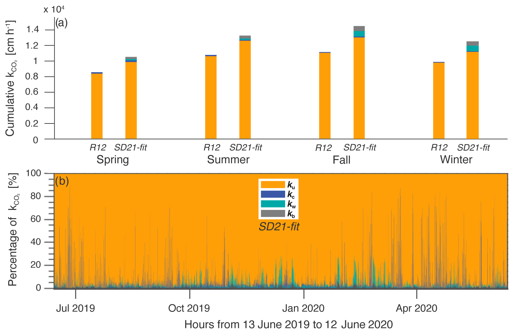
Figure 7 (a) Distribution of $k_{{\mathrm{CO}}_{\mathrm{2}}}$ generated by two main processes (k_u and k_c) in R12 and four main processes (k_u, k_c, k_w, and k_b) in SD21-fit for each season: spring (April–May–June), summer (July–August–September), fall (October–November–December), and winter (January–February–March). The height of the bar represents the cumulative $k_{{\mathrm{CO}}_{\mathrm{2}}}$ by season for both models (R12 and SD21-fit). (b) Distribution of four k generated by wind shear, convection, wave action, and bubble enhancement (k_u, k_c, k_w, and k_b respectively) along the annual cycle. For the SD21-fit model, k_u=SRM(ε_u), $k_{\mathrm{c}}=\text{SRM}({\mathit{\epsilon }}_{\mathrm{u}}+{\mathit{\epsilon }}_{\mathrm{c}}+{\mathit{\epsilon }}_{\mathrm{w}})-\text{SRM}({\mathit{\epsilon }}_{\mathrm{u}}+{\mathit{\epsilon }}_{\mathrm{w}})$, $k_{\mathrm{w}}=\text{SRM}({\mathit{\epsilon }}_{\mathrm{u}}+{\mathit{\epsilon }}_{\mathrm{c}}+{\mathit{\epsilon }}_{\mathrm{w}})-\text{SRM}({\mathit{\epsilon }}_{\mathrm{u}}+{\mathit{\epsilon }}_{\mathrm{c}})$, and k_b.

Wind shear remains the dominant component of the gas exchange velocity over the different seasons (Fig. 7a). The annual contribution of surface waves (wave action and bubble formation) is limited to 9 %–10 % of the cumulative k in fall and winter. The contribution of the buoyancy flux at the surface to k is even smaller for both models (R12 and SD21-fit) at this seasonal scale. However, both the buoyancy flux and the surface waves can significantly increase k during episodic events, during which they can contribute disproportionately to k at hourly (up to 80 % for convection) and daily (up to 25 % for surface waves) timescales (Fig. 7b). Several studies have emphasised the disproportionate contribution of episodic mixing events to the annual flux, bringing CO₂ back to lake surfaces such as after ice break in dimictic lakes (Karlsson et al., 2013; Finlay et al., 2019) or during fall mixing in a eutrophic deep lake (Reed et al., 2018). Process-based k models integrating both the buoyancy flux and the wind-induced waves offer the opportunity to mechanistically investigate how much these episodic events contribute to annual emissions through short-term modifications of the gas exchange velocity.

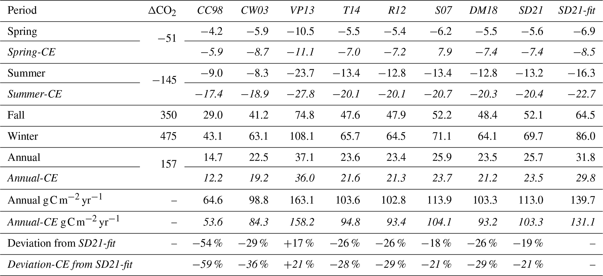
Table 3 Seasonal to annual CO₂ flux estimation ($\mathrm{mmol}\mathrm{C}{\mathrm{m}}^{-\mathrm{2}}{\mathrm{d}}^{-\mathrm{1}}$) from k models (with, denoted using “-CE” (italic font), and without (roman font) chemical enhancement), the monthly ΔCO₂ average (µatm), and the models' deviation from SD21-fit. CE was only considered for seasons when pH > 8.4.

4.2.2 Consequences of the choice of k model on the seasonal to annual CO₂ flux estimation

We produced coarse estimates of monthly CO₂ fluxes with the objective of scaling the effects of wave integration at seasonal and annual scales. Monthly fluxes were computed based on k estimates at LéXPLORE from the different models at an hourly time step as well as the monthly average of water temperature and recorded pCO₂ at the lake surface (OLA-IS, AnaEE-France, INRAE of Thonon-les-Bains, CIPEL; Rimet et al., 2020; Perga et al., 2016) as well as a constant pCO₂ in the atmosphere (400 µatm). For months for which surface pH > 8.4,k values were computed with and without considering the chemical enhancement (CE; Wanninkhof and Knox, 1996) (Table 3). The dependency of the chemical enhancement factor on k (Wanninkhof and Knox, 1996) might generate a further uncertainty in estimated CO₂ fluxes (e.g. with a greater k value being related to a lower chemical enhancement factor).

As predicted by Fick's law, the highest outgassing fluxes occur in fall and winter, when water mixing brings CO₂ up to the lake surface, whereas low gas uptake fluxes occur in spring and summer, when primary production depletes surface CO₂ below saturation. However, annual estimates of net CO₂ outgassing vary from 14.7 to 37.1 $\mathrm{mmol}\mathrm{C}{\mathrm{m}}^{-\mathrm{2}}{\mathrm{d}}^{-\mathrm{1}}$ (Table 3) depending on the k model used for computation. Consistently, differences between model estimates are relatively low in summer, as both the ΔpCO₂ gradient (100–200 µatm) and wave occurrence are limited. Adding CE during the spring and summer months causes an increase in influx of the order of 5 %–128 % depending on the k model used. For example, using CC98 in summer leads to a 93 % increase in the estimated influx (compared with fluxes without CE), whereas the increase is only 39 % for SD21-fit. This chemical enhancement factor deserves more attention in future studies, especially for high pH lakes and summer seasons. However, the variability introduced by the CE at the annual scale remains low (∼10 %) compared with that introduced by the choice of the k model. Estimated fluxes are also strongly dependent on the chosen k model in winter when both ΔpCO₂ (475 µatm) and surface wave occurrence are higher (Fig.7, Table 3). Therefore, while high-wave events represent only 6 % of the total surface wave occurrence (H_s > 0.4 m), an incomplete consideration and description of their contribution may lead to an annual flux underestimation of about 20 %–25 %.

The weak contribution of convection is at odds with observations in small lakes, although not unexpected, as large lakes are exposed to stronger winds, such that wind-shear-driven ε_u often outpaces convectively driven ε_c (Read et al., 2012). However, the limited impact of the buoyancy flux on k does not rule out its contribution to CO₂ exchange. Indeed, convective mixing plays a central role in the deepening of the mixed layer, allowing the export of the CO₂ stored in the hypolimnion towards the surface during the cold period and, thus, controlling the pCO₂ gradient (Zimmermann et al., 2019) and the observed wintertime outgassing. Altogether, both surface oversaturated CO₂ concentrations (as a result of convective mixing) and wind-induced waves are more relevant in fall and wintertime for the monomictic Lake Geneva, leading to most of the annual outgassing during this season (Table 3). As for many monomictic lakes, these seasons drive most of the annual CO₂ budget of Lake Geneva (Perga et al., 2016), whereas they usually correspond to those where direct measurements are the scarcest. An improved quantification of k values through SRM models including wind-induced waves should contribute to refining the overall estimation of large lakes' contribution to regional CO₂ emissions.

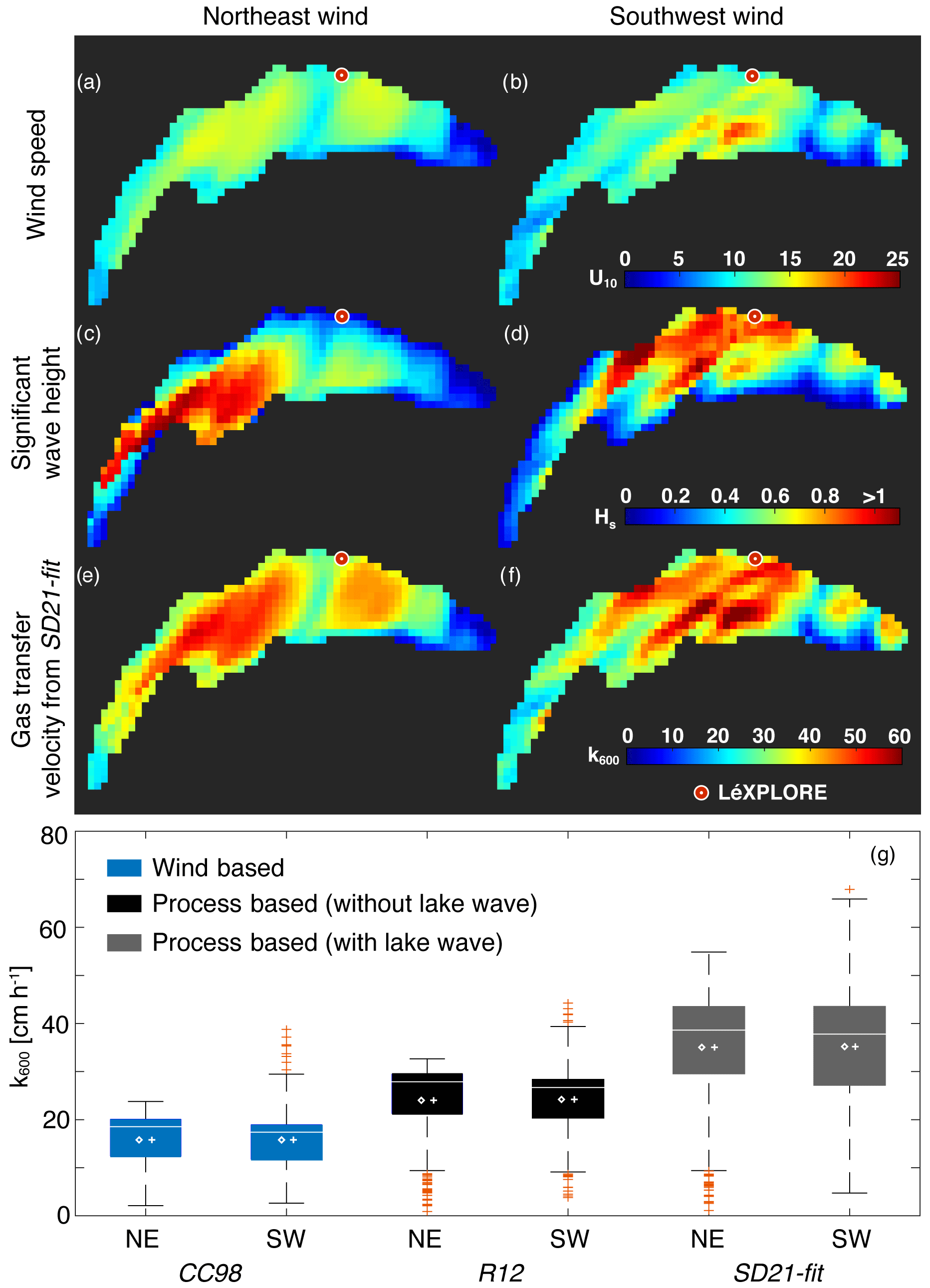
Figure 8 (a, b) Wind fields from COSMO-1 for two episodes of northeast and southwest wind directions; (c, d) wave fields on Lake Geneva considering the two prevailing winds (northeast and southwest); (e, f) gas transfer velocity from SD21-fit; (g) boxplots of the spatial variability, at the lake scale, of k values computed from CC98, R12, and SD21-fit under both meteorological conditions. Diamonds represents the spatial mean, and the cross (+) represents the k value computed from the averaged fetch distance (NE: 9.5 km; SW: 9.3 km).

4.3 Wind and wave field on Lake Geneva and their impact on the spatial integration of k₆₀₀

SD21 and SD21-fit were built on the basis of a single measurement point on the lake, just as for most of the existing k models. Therefore, the question of the extrapolation of the model to the whole lake remains essential. Herein, we showcase two snapshot situations of high wind (i) to illustrate how process-based models could enable spatially resolved estimates of k values and (ii) to exemplify how much k can vary as a result of the spatially variable wave and wind fields during a single episode. Two events of high and similar wind speed (11 m s⁻¹) but different directions (NE on 30 March 2020 at 08:00 UTC and SW on 10 February 2020 at 06:00 UTC; Fig. 8a, b) were extracted from the 0.01^∘ hourly resolved numerical weather model of the Swiss Federal Office of Meteorology and Climatology (COSMO-1, MeteoSwiss). The two fetch distances from both prevailing wind directions (NE, SW) were then measured at each pixel of the grid (n=583), from which the wave height field was mapped (Fig. 8c, d) considering Eq. (3) and the two wind grids. The maps were qualitatively consistent with previous studies on wind waves for Lake Geneva using the spectral wave model (SWAN) for wave height (Amini et al., 2016). Spatially resolved k values were computed from the fetch and wind grids, using the wind-based model CC98, the process-based model without lake wave implementation R12, and the SD21-fit model containing the lake wave parameterisation.

Taking H_s > 0.4 m as a threshold for the significant effect of waves on k, the two prevailing winds show opposite wave responses, with long fetch and higher wave heights affecting either the northern or the southern shores for the SW and NE winds respectively. Under both conditions, more than 60 % of the full lake surface area experiences H_s values > 0.4 m, leading to k values as high as 68 cm h⁻¹ as computed by SD21-fit (Fig. 8g). The eastern part of lake experiences the lowest wind speeds and wave heights in both situations, as a consequence of the orographic effect of the Alps surrounding the Grand Lake.

Both the range and the mean of estimated k values increase with increasing model complexity. Accounting only for wind speed, through the wind-based model CC98, leads to a spatially integrated k value of 15.7 cm h⁻¹ (range of 1–22 cm h⁻¹). k values computed from R12, accounting for both the wind shear and buoyancy flux, are on average 55 % greater (24.3 cm h⁻¹) with a moderate effect on the range of spatial variability. Finally, including surface waves results in a spatially averaged k value that is more than double the k value computed from wind speed only (35.5 cm h⁻¹), with a variability that is almost 3 times greater (range of 0–68). It is noteworthy that the spatial average of the k values computed by the wind grids (Fig. 8g, diamonds) is equivalent to the average of k values computed from the spatial mean fetch (9.5 km for NE and 9.3 km for SW; Fig. 8g, crosses) under these specific weather conditions. Thus, the application of an average fetch would be relevant to estimate a spatially averaged k value.

For all models, the integration of spatially resolved wind fields may improve the accuracy of k at the lake scale, but accounting for wind only would underestimate both the average gas piston velocity and its spatial variability. Therefore, a better understanding of wave behaviour in large lakes, using different approaches such as field and laboratory measurements, new physical models, and technical development, would improve the accuracy of gas exchange estimates at the lake–water interface, at both temporal and spatial scales. Further, estimates of lake-scale CO₂ fluxes would also require one to account for the spatial variability of CO₂. The question of the spatial variability of the ΔCO₂ is still open and remains difficult to analyse at high frequency in large lakes.

5 Conclusions

Investigations of the four main processes generating the gas transfer velocity in the large Lake Geneva demonstrated the importance of considering surface waves during episodic windy events responsible for more than 44 % of annual cumulative k₆₀₀. The in-depth study of the behaviour of the process-based models has enabled us to underscore their consistent predictions under low and strong wind conditions, especially considering the new combination and adaptation model, SD21-fit. This last model significantly improves the estimation of the CO₂ flux when these three thresholds appear in the field, U₁₀ > 5 m s⁻¹, Fetch > 15 km, and H_s > 0.4 m, making it applicable to a wide range of lake sizes. Furthermore, SD21-fit is assembled on solid theoretical bases coming from limnological and oceanic literature and allows one to analyse the distribution of these four main terms (k_u, k_c, k_w, and k_b) across a variety of timescales depending on the kind of study.

To conclude, the development of high-resolution gridded atmospheric models such as COSMO-1 is an asset for future estimates of the gas transfer velocity and the spatial heterogeneity of lake biogeochemical cycles. Moreover, this study sheds light on the complexity of large lakes located at the interface between small, sheltered lakes and the open oceans, experiencing a combination of processes relevant for both small and large systems. The possibility of using process-based models in a fairly simple way with few inputs to improve the precision of the gas transfer velocity and, therefore, the gas flux should be supported in future research. In addition, this approach is very promising with respect to uncovering long-term trends of CO₂ emissions from lakes as well as for finer estimation of fluxes during more intense episodic events.

Appendix A

Figure A1 Schematics of eosFD operation (https://eosense.com, last access: 18 August 2020), its mini-platform construction, and its positioning for measurements in the field (Lake Geneva at LéXPLORE platform). The raft design also complies with recommendations to minimise artificial turbulence induced by the chamber's walls, with 10 cm long-edges entering the water (Vachon et al., 2010).

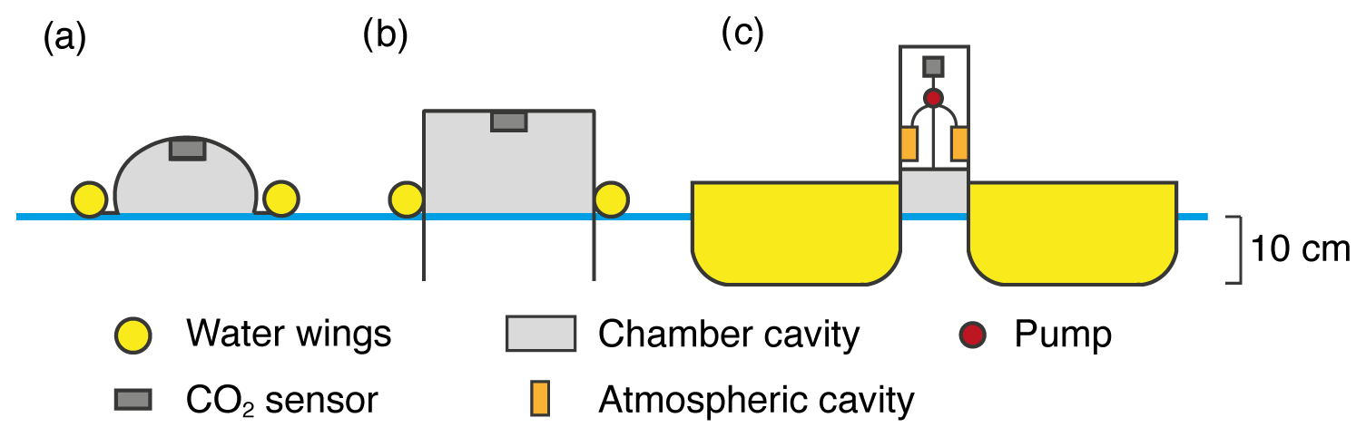
Figure A2 (a) Classical floating chamber; (b) floating chamber with 10 cm long-edges; (c) platform design used in this study: 10 cm long-edges, rounded-edges, and flat and long water wings.

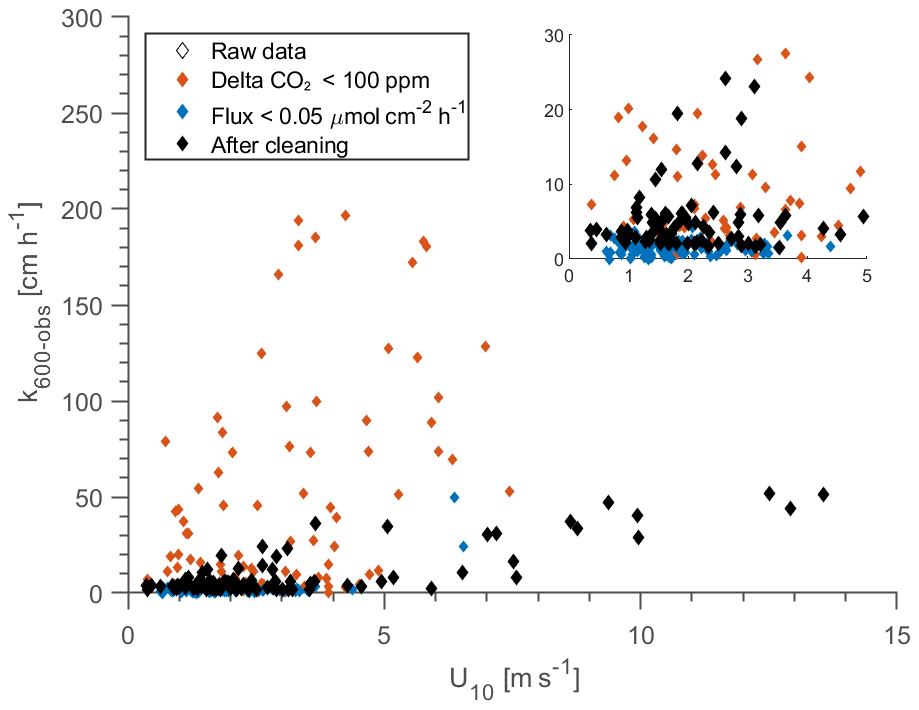
Figure A3 Visualisation of 304 observed k₆₀₀ values during the five periods of flux measurements: 13–14 June 2019, 27–28 August 2019, 1–5 October 2019, 18–20 December 2019, and 20–26 February 2020.

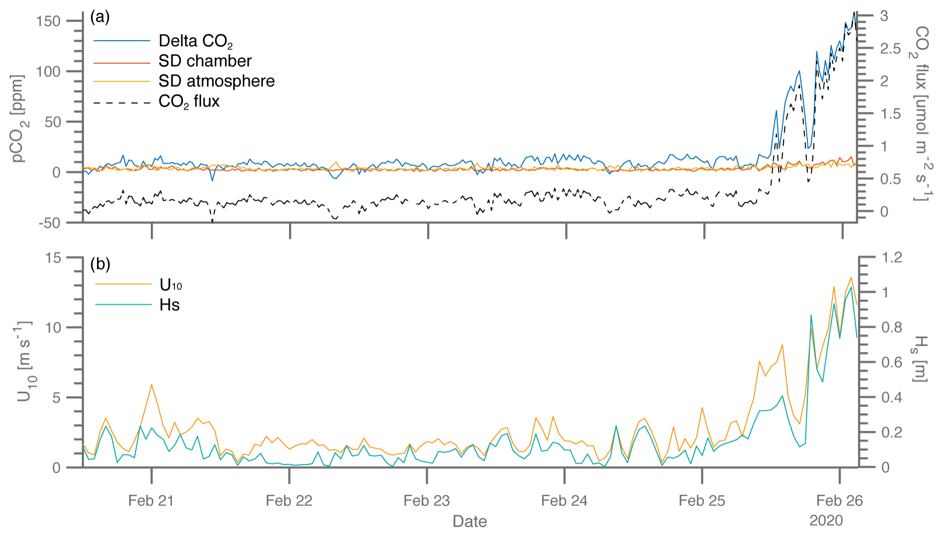
Figure A4 (a) Raw outputs of the eosFD during one period of CO₂ flux measurements, showing the ΔCO₂ between both cavities of measures (atmosphere cavity and chamber cavity) (blue line); the standard deviation of each cavity between two automated flushing events (30 min of interval) – chamber cavity (red line) and atmosphere cavity (yellow line); and the CO₂ flux (black dash line). (b) Temporal evolution of U₁₀ and H_s during the same period as the CO₂ flux measurements. The increase in flux on 25 February corresponds to the increase in wind speed and waves.

Appendix B

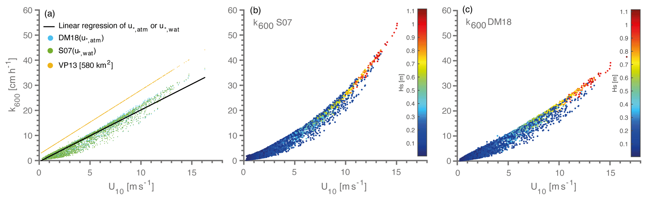
Figure B1 Panel (a) shows the comparison of Soloviev et al. (2007) and Deike and Melville (2018) for the first-order function of friction velocity at the water side ($u_{\ast ,\text{wat}}$) (blue points) and at the atmosphere side ($u_{\ast ,\text{atm}}$) (green points) with their linear regression (black line), the linear function of Vachon and Prairie (2013) for a lake size of 582 km² (yellow points), and the linear regression from $u_{*,\mathrm{wat}}$ or $u_{*,\mathrm{atm}}$. Panel (b) is a visualisation of S07 with empirical parameterisation of the bubble term (Woolf, 1997) regardless of wave height as a function of wind speed at 10 m. Panel (c) is a visualisation of DM18 as a function of wind speed, only using the effect of the bubble term from 10 m s⁻¹.

Appendix C

Figure C1 Annual evolution of three main inputs of k models: wind speed at 10 m (U₁₀), buoyancy flux at surface (B₀), and significant wave height (H_s).