Impact of environmental changes and land management practices on wheat production in India

Spring wheat is a major food crop that is a staple for a large number of people in India and the world. To address the issue of food security, it is essential to understand how the productivity of spring wheat varies with changes in environmental conditions and agricultural management practices. The goal of this study is to quantify the role of different environmental factors and management practices on wheat production in India in recent years (1980 to 2016). Elevated atmospheric CO₂ concentration ([CO₂]) and climate change are identified as two major factors that represent changes in the environment. The addition of nitrogen fertilizers and irrigation practices are the two land management factors considered in this study. To study the effects of these factors on wheat growth and production, we developed crop growth processes for spring wheat in India and implemented them in the Integrated Science Assessment Model (ISAM), a state-of-the-art land model. The model is able to simulate the observed leaf area index (LAI) at the site scale and observed production at the country scale. Numerical experiments are conducted with the model to quantify the effect of each factor on wheat production on a country scale for India. Our results show that elevated [CO₂] levels, water availability through irrigation, and nitrogen fertilizers have led to an increase in annual wheat production at 0.67, 0.25, and 0.26 Mt yr⁻¹, respectively, averaged over the time period 1980–2016. However, elevated temperatures have reduced the total wheat production at a rate of 0.39 Mt yr⁻¹ during the study period. Overall, the [CO₂], irrigation, fertilizers, and temperature forcings have led to 22 Mt (30 %), 8.47 Mt (12 %), 10.63 Mt (15 %), and −13 Mt (−18 %) changes in countrywide production, respectively. The magnitudes of these factors spatially vary across the country thereby affecting production at regional scales. Results show that favourable growing season temperatures, moderate to high fertilizer application, high availability of irrigation facilities, and moderate water demand make the Indo-Gangetic Plain the most productive region, while the arid north-western region is the least productive due to high temperatures and lack of irrigation facilities to meet the high water demand.

1 Introduction

Wheat is a major food crop and is ranked third in India and fourth in the world in terms of its production (FAOSTAT online database, 2019). Wheat can be of two main types: winter and spring wheat. Winter wheat undergoes a 30–40 d long vernalization period induced by below-freezing temperatures and hence has a longer growing season of 180–250 d. In contrast, spring wheat, which does not undergo vernalization, has a growing season of 100–130 d (FAO Crop Information, 2018). In India, spring wheat is sown during October–November and harvested during February–April (Sacks et al., 2010). It is grown in widely divergent climatic conditions across the country where different environmental factors like temperature, water availability, and [CO₂] may affect growth and yield. Ideally, a daily average temperature range of 20–25 ^∘C is ideal for wheat growth (MOA, 2016). Studies have reported heat stress in wheat for temperatures between 25 to 35 ^∘C (Deryng et al., 2014) during the grain development stages. Beyond the temperatures of 35 ^∘C, wheat fails to survive. High temperatures are terminal to wheat yield specifically in the flowering and grain filling stages during the second half of the growing season (Farooq et al., 2011). Increasing temperature change and heat stress events in recent decades and their impacts on wheat crop growth processes have been extensively studied (Asseng et al., 2015; Lobell et al., 2012; Farooq et al., 2011; Ortiz et al., 2008). Another environmental factor that has been widely studied is the impact of increasing [CO₂]. The resulting CO₂ fertilization effect is found to promote crop growth (Dubey et al., 2015). Apart from environmental factors, management practices including nitrogen fertilizer application and irrigation also significantly affect wheat production (Myers et al., 2017; Leaky et al., 2009; Luo et al., 2009). Because wheat is grown in the non-monsoon months, it is a high irrigation crop with almost 94 % of the wheat fields in India equipped for irrigation (MAFW, 2017). The quantification of the impacts of land management practices on crop growth helps in understanding how croplands can be managed to improve production (Tack et al., 2017).

Even though India is the third largest wheat producer in the world, domestic production is barely sufficient to meet the country's demand for food and livestock feed (USDA, 2018). Data from different sources report a relatively poor yield of wheat in India as compared to other countries (FAOSTAT online database, 2019). Hence, there is an urgent need to address this yield gap by developing better land management practices under different environmental conditions (Stratonovitch and Semenov, 2015; Zhao et al., 2014; Luo et al., 2009). A key first step to achieve this goal is to understand the processes involved in interactions of the crop with its environment and the factors responsible for impacting crop growth.

Dynamic global vegetation models (DGVMs) are well-established tools to study global climate–vegetation systems. Implementation of crop-specific parameterization and processes in DGVMs provides us with a better framework to assess and represent the role of agriculture in climate–vegetation systems (Song et al., 2013; Bondeau et al., 2007). This improves the representation of biogeochemical and biogeophysical processes, especially the feedback mechanisms, and the prediction of crop yield and production. Multiple process-based models with crop-specific representations are currently being used (e.g. Lu et al., 2017; Drewniak et al., 2013; Song et al., 2013; Lokupitiya et al., 2009; Bondaeu et al., 2007) instead of stand-alone crop models for this purpose.

This study explores the effects of environmental drivers and management practices on spring wheat in India using the Integrated Science Assessment Model (ISAM) (Song et al., 2015, 2013). The specific objectives of this study are (1) to implement a dynamic spring wheat growth module in ISAM and (2) to study the effect of environmental factors (elevated [CO₂] and climate change, including temperature and precipitation change) and land management practices (irrigation and nitrogen fertilizers) on the production of spring wheat in India for the 1980–2016 period using ISAM. To the best of our knowledge, this is the first study that evaluates the impacts of multiple environmental factors and land management practices on spring wheat in India at a country level by implementing spring wheat specific processes in a land surface model.

2 Methods

2.1 Study design

The study is designed as follows. First, field data on crop physiology are collected at an experimental spring wheat field site. Next, the spring wheat model is developed and implemented in ISAM. The model is run at site scale for the calibration and evaluation of the site data. Next, the model is run for the entire country and evaluated with country-scale wheat production data. Finally, numerical experiments are conducted to estimate the effects of various environmental factors and land management practices on spring wheat production. Details of each step are described below.

2.2 Site data

Field data on spring wheat growth are required to develop, calibrate, and evaluate the spring wheat model. Such data are not readily available in the public domain. Hence, a field campaign is conducted during two growing seasons: 2014–2015 and 2015–2016. Leaf area index (LAI) is measured for 2014–2015, and LAI and above-ground biomass at different growth stages are measured for the growing season 2015–2016 at a wheat experimental site. The site is approximately 650 m² in area and is located at 28^∘40^′ N, 77^∘12^′ E in the Indian Agricultural Research Institute (IARI) campus in New Delhi, which is a subtropical, semi-arid region. The crop was sown on 18 November 2014 and 20 November 2015. It reached physiological maturity on 30 March in both years. The wheat field is irrigated with an unlimited amount to ensure that the water stress to the crop is minimal. Mimicking local farming practices, whenever the soil is perceived to be dry, water is added till the top layers are near saturated. These led to four irrigation episodes in 2014–2015 and five in 2015–2016. A total amount of nitrogen fertilizer of 120 kg N ha⁻¹ is added to the crop in three batches of 60, 30, and 30 kg N ha⁻¹ in a span of 60 d from planting day.

The LAI is measured at weekly intervals with LI-COR's LAI-2000 plant canopy analyser that measures gap fraction at five zenith angles using hemispherical images from a fisheye camera. LAI is estimated by comparing one above-canopy and three below-canopy measurements. The observed LAI is actually an average of multiple (at least five) LAI observations at different locations in each plot. To measure above-ground biomass, plant samples from 50 cm row length are first cut just above the soil surface. Then, different plant organs like leaves, stem, and spike (after anthesis) and portions of plant samples are separated out. These are initially dried in the shade and later dried at 65 ^∘C in an oven for 72 h till the weight stabilizes. Finally, the weight of dried plant samples is measured using an electric balance. To measure yield, two samples of mature wheat crops are harvested from 1 m×1 m area in each plot and allowed to air dry. The total weight of grains and straw in each plot is recorded with the help of a spring balance. After thrashing and winnowing by mechanical thrasher, grains are weighed to estimate grain yield and thousand grain weight.

2.3 Model description

2.3.1 Dynamic C₃ crop model in ISAM

ISAM is a well-established land model that has been used for a wide range of applications (Gahlot et al., 2017; Song et al., 2016, 2015, 2013; Barman et al., 2014a, b). ISAM simulates water, energy, carbon, and nitrogen fluxes at a 1-hour time step with $\mathrm{0.5}{}^{\circ }\times \mathrm{0.5}{}^{\circ }$ spatial resolution. ISAM has vegetation-specific growth processes for all major plant-functional types implemented in the model to better capture seasonality for each. Song et al. (2013) have developed a soybean and maize model for ISAM. Because soybean and wheat are both C₃ crops, the dynamic C₃ crop model framework from the soybean model is used as a foundation to build a spring wheat model for this study. The model structure, phenological stages, carbon, and nitrogen allocation processes, parameters, and performance have been extensively described and evaluated in various studies (Song et al., 2016, 2015, 2013).

2.3.2 Development and implementation of spring wheat processes in ISAM

The spring wheat processes in ISAM are implemented using the C₃ crop framework (Song et al., 2013). For this purpose, C₃ crop specific equations and parameters are updated based on the literature. The model equations are available in Song et al. (2013). A brief description is given in the Supplement, and the revised parameters are available in Table S1 in the Supplement. Some of the parameter values are collected from the literature while the rest are estimated during model calibration.

ISAM accounts for dynamical planting (Song et al., 2013). This unique feature of ISAM is quite important for modelling wheat in India because in India wheat is grown in different climatic conditions (Ortiz et al., 2008) and in multiple cropping systems. In the rain-dependent, tropical, central parts of India, wheat is planted early; in eastern parts of India, where rice is harvested before the wheat is planted on the same field, wheat is planted late; and it is timely sown in the northern and western parts of India (Table S2). ISAM uses different conditions based on a 7 d average of air temperature and 30 d total precipitation to dynamically calculate the planting day. Observed wheat planting and harvest dates (Sacks et al., 2010) are used to calibrate the planting time and harvest time criteria in the model along with other state-level and regional datasets (NFSM, 2018). This allows for the correct simulation of the observed spatial variability of the planting date.

The heat stress effect is implemented to account for the observed negative effects of high temperatures on grains (Asseng et al., 2015; Farooq et al., 2011) during the reproductive stage of the phenology (Zhao et al., 2007). To include these effects, net carbon available for allocation to grains decreases as daily average temperatures increase from 25 to 35 ^∘C in the flowering and grain filling stages (Table S3; Eqs. S1–S3). This limits the growth of a plant. Beyond daily average temperatures of 35 ^∘C, the grains fail to develop.

2.4 Site-scale simulations for calibration and validation

The spring wheat model is calibrated at site level using LAI and above-ground biomass data collected at the IARI site for the 2015–2016 growing season using the protocol described in Song et al. (2013) and validated using LAI data for the 2014–2015 growing season. ISAM can be configured to run for a single point. Using this capability, ISAM is run at site scale to simulate spring wheat growth observed at the IARI site.

The model is spun up by recycling the Climate Research Unit–National Centers for Environment Prediction surface climate data (CRU-NCEP; Vivoy, 2018), Global Carbon Project Budget 2017 [CO₂] data (Le Quéré et al., 2018), and the airborne nitrogen deposition data (Dentener, 2006) for 2015–2016 until the soil temperature, soil moisture, the soil carbon pool, and the soil nitrogen pool reach a steady state. Then, the above-ground biomass carbon (leaves + stem + grain) is calibrated using above-ground biomass (Fig. 1a), nitrogen fertilizer amount added, sowing date, and harvest date for the 2015–2016 growing season. Next, phenology-dependent carbon allocation fractions for leaves, stem, and grain are calibrated using the LAI data (Fig. 1b), duration, and heat unit index requirement for each growth stage. The model is evaluated by comparing simulated and observed LAI for the 2014–2015 growing season.

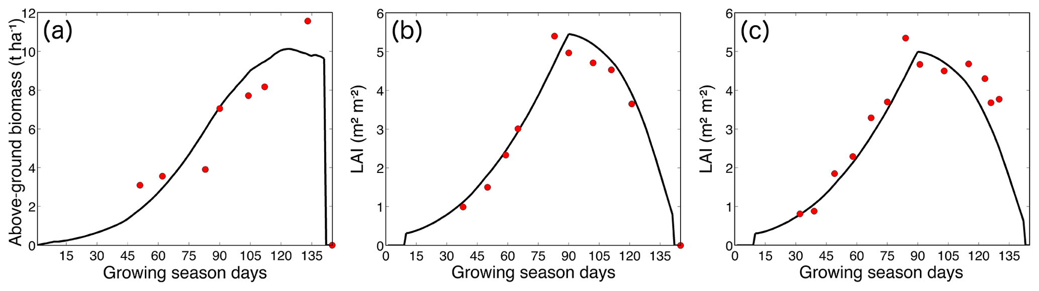
Figure 1 Model calibration and validation plots for the experimental wheat site at IARI, New Delhi. (a) Model calibration for above-ground biomass for the 2015–2016 growing season. (b) Model calibration for LAI for the 2015–2016 growing season. (c) The model-estimated LAI validated with site-measured data for the 2014–2015 growing season. The red dots are site-measured values and the black lines are ISAM-simulated values.

2.5 Gridded data for country-scale simulations

Driver data for environmental and anthropogenic forcings are required to conduct ISAM simulations. ISAM is driven by $\mathrm{0.5}{}^{\circ }\times \mathrm{0.5}{}^{\circ }$ surface climate data from CRU-NCEP (Viovy, 2018) with 6-hourly temperature, specific humidity, incoming short-wave and long-wave radiation, wind speed, and precipitation rate that are interpolated to hourly values. Annual [CO₂] data are taken from the Global Carbon Project Budget 2017 (Le Quéré et al., 2018). Spatially explicit annual nitrogen fertilizer data for wheat from 1901 to 2005 are created by combining nitrogen fertilizer data from Ren et al. (2018) and Mueller et al. (2012) (Table S3; Eqs. S4–S5).

Gridded data for the wheat harvested area, nitrogen fertilizer application, and irrigation are required as model input to estimate actual wheat production for India in recent years (1980–2016). For this purpose, an annual, spatially explicit gridded wheat harvested area dataset for India is created as part of this study by combining spatially explicit wheat area from Monfreda et al. (2008) for the mean value over the time period 1997–2003 (ca. 2000) and non-gridded state-specific annual wheat harvested area from the Directorate of Economics and Statistics, Ministry of Agriculture and Farmers Welfare, India (MAFW, 2017) (Eqs. S6, S7, S8). The annual area equipped for irrigation (AEI) dataset is created by linear interpolation of decadal data from Siebert et al. (2015) (Eq. S9).

2.6 Country-scale simulations

Country-scale simulations are conducted after model calibration and evaluation. First, we spin up the model for the year 1901 until the soil temperature, soil moisture, and the soil carbon and nitrogen pools reach a steady state at approximately 1901 levels. For the spin-up run, the model is driven by recycled CRU-NCEP (Viovy, 2018) climate data for the period 1901–1920, while [CO₂] (Le Quéré et al., 2018) and airborne nitrogen deposition (Dentener, 2006) are kept fixed at 1901 levels, and nitrogen fertilizer and irrigation are set to zero. Details of the spin-up process are described in Gahlot et al. (2017). After the model spin-up, numerical experiments are conducted as transient runs from 1901 to 2016. To estimate the effects of external forcings, country-scale runs are conducted over wheat-growing regions in India by varying different input forcings (Table 1). The control run (S_CON) represents the model run from 1901 to 2016 with time-varying annual [CO₂], climate data, annual grid-specific nitrogen fertilizer, and full irrigation to fulfil the water needs of the crop. Four additional simulations are conducted by assigning a constant value to each input forcing one at a time. For instance, in $S_{{\mathrm{CO}}_{\mathrm{2}}}$, all input variables (temperature, nitrogen, and irrigation) are the same as in the S_CON case except [CO₂], which is held constant at the 1901 level. The difference in model simulations from S_CON and $S_{{\mathrm{CO}}_{\mathrm{2}}}$ then gives the effect of elevated [CO₂] on wheat crop growth processes. Here we present the results only for the recent decades of 1980 to 2016.

Table 1 Description of numerical experiments conducted with ISAM wheat model from 1901 to 2016. The text in bold font highlights the special characteristics of the experimental simulations.

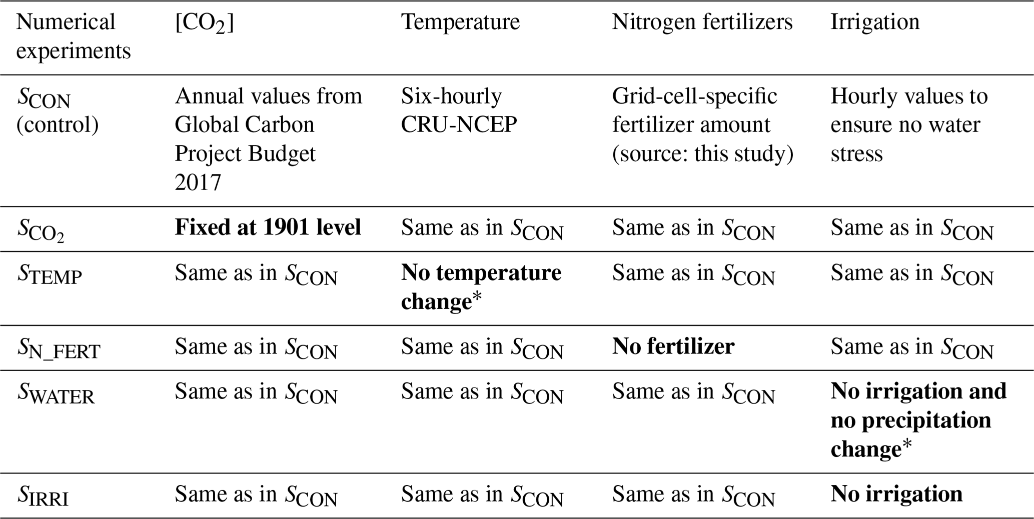
^∗ Data for years 1901–1930 are recycled to represent stable (no change) conditions.

Model performance at the country scale is evaluated by comparing the model simulated total wheat production at the country level with the FAOSTAT online database (2019) and the Directorate of Economics and Statistics, Ministry of Agriculture and Farmers Welfare (MAFW, 2017) data. The production for each grid cell is an area-weighted sum of production from irrigated and rainfed area fractions (Eq. S10).

Table 2 Characteristics of different spring wheat environments (SWEs) in India.

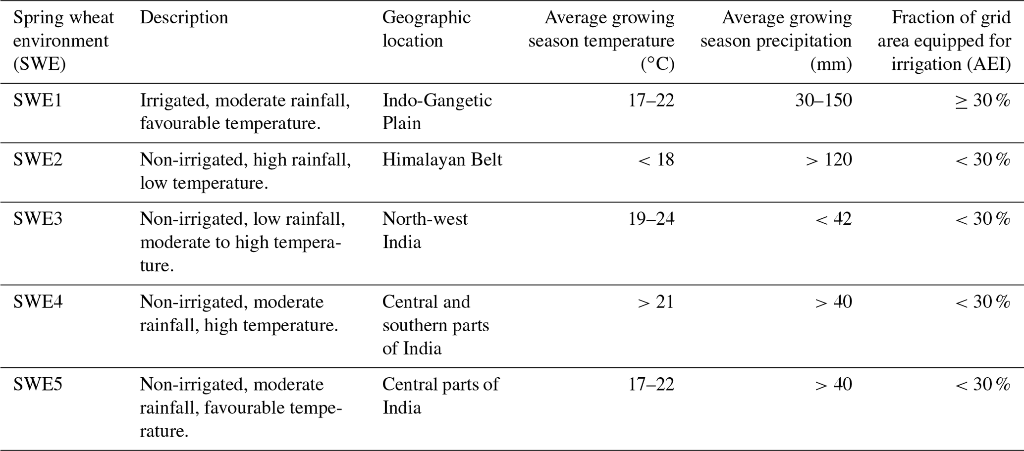
To study the spatial variation in production, the wheat-growing regions of India are divided into spring wheat environments (SWEs) based on the mega-environment concept (Chowdhury et al., 2019). For this purpose, we divide the wheat-growing regions of India into five SWEs (Fig. 2) based on temperature, precipitation, and area equipped for irrigation (Table 2) to identify regions with similar growing conditions for wheat. SWE1 (Fig. 2) represents mostly the Indo-Gangetic Plain that offers good access to irrigation for wheat, which is a non-monsoon crop. The growing season temperatures fall in the optimum range for wheat growth. SWE2, which is mainly comprised of the wheat-growing regions in the proximity of the Himalayas, is characterized by very low growing season temperatures and high rainfall. SWE3 represents the north-western parts of the country with moderate to high growing season temperatures, low rainfall, and small values of AEI. SWE4 represents the central parts of India and tropical wheat-growing regions with high temperatures and moderate growing season precipitation. SWE5 represents the crucial wheat-growing regions of the country where the conditions are similar to SWE1 but irrigation facilities are lacking. Wheat production for each of the SWEs are discussed further in the following sections.

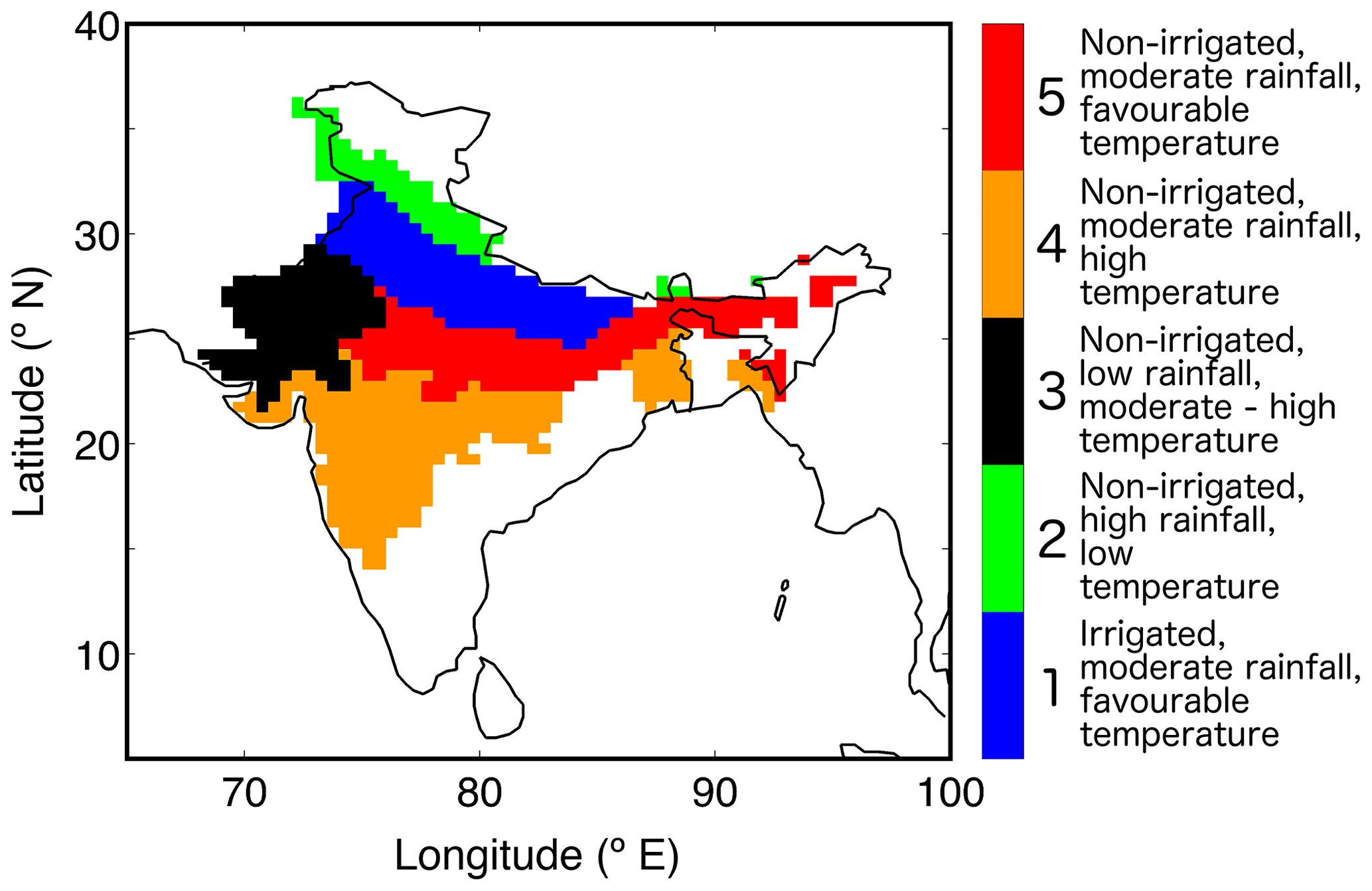
Figure 2 Classification of wheat-growing areas into spring wheat environments in India.

3 Results

3.1 Spring wheat model evaluation

The simulated magnitude and intra-seasonal variability in LAI for 2014–2016 compared well with the experimental wheat site at IARI, New Delhi (Fig. 1c).

The spatial distribution of the model-estimated wheat production at a country scale compared well, including the highly productive Indo-Gangetic Plain, with the data from Monfreda et al. (2008) for the year 2000 (Fig. 3). ISAM-simulated country-scale wheat production for 1980–2014 also compares well with production data from the FAOSTAT online database (2019) and MAFW (2017) datasets (Fig. 4) with correlation coefficients of 0.92 and 0.91, respectively, for the two datasets. However, the model-estimated production is slightly higher than both observed datasets. This may be attributed to the fact that the model is calibrated to the high-yielding wheat cultivars grown in recent years (2015–2016). Hence, the model is a valid tool for studying interactions of wheat with its environment for recent years.

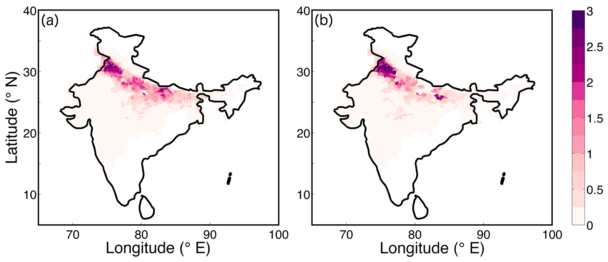
Figure 3 Wheat production (×10⁴ t) averaged for 1997–2003 (a) simulated by ISAM and (b) observed in the M3 dataset (Monfreda et al., 2008).

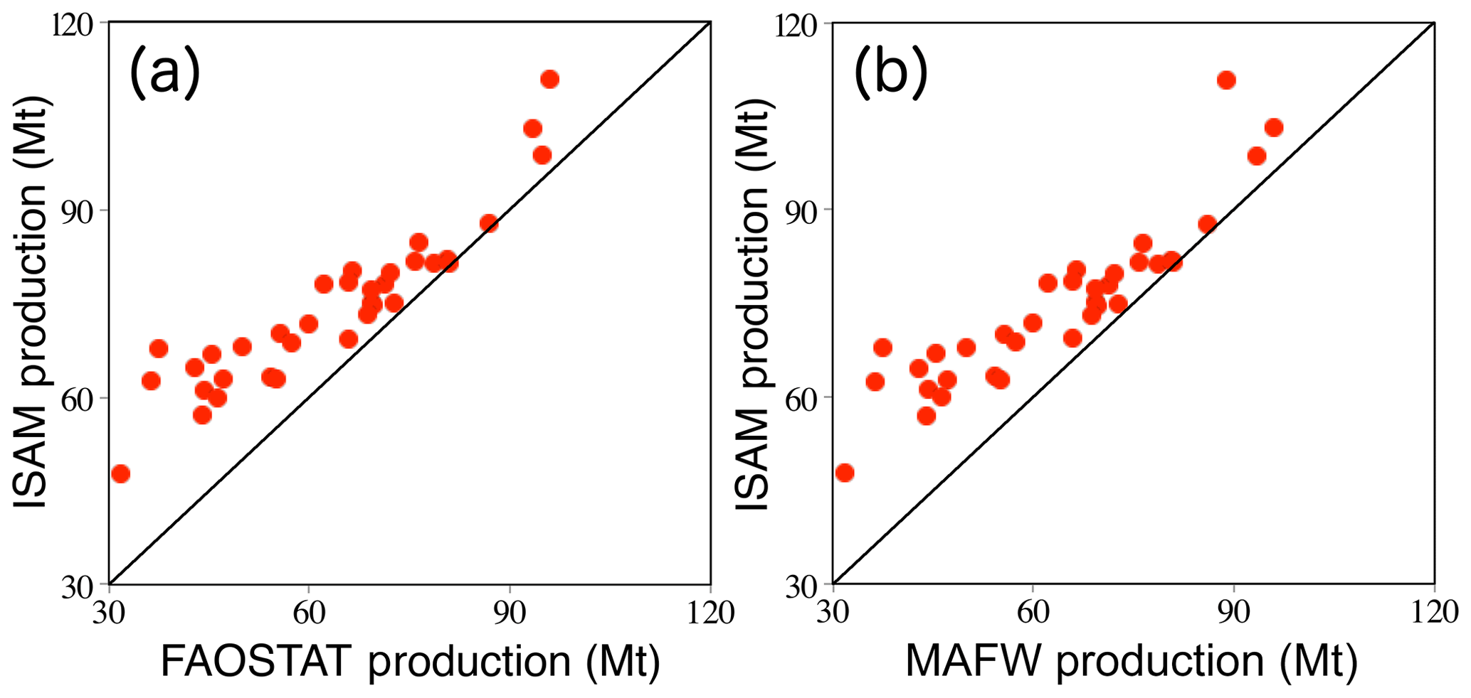
Figure 4 Scatter plots of the ISAM-simulated wheat production (Mt) compared to (a) FAOSTAT (2019) and (b) the Directorate of Economics and Statistics, Ministry of Agriculture and Farmers Welfare, India (MAFW, 2017) datasets from 1980 to 2014. The Pearson's correlation coefficients are (a) 0.92 and (b) 0.91.

3.2 Effects of environmental and anthropogenic forcings at the country scale

In this study, we examine the effects of two environmental factors ([CO₂] and temperature change) and two land management practices (nitrogen fertilizer and water availability) on the production of spring wheat. The impact of these factors is quantified as the difference between the control and the experimental simulations (Eq. S11) described in Table 1. Results show that during the 1980–2016 period, [CO₂], nitrogen fertilizers, and water available through irrigation have a positive impact on wheat production, but the impact of temperature is negative (Fig. 5) due to reasons detailed below. The effects of [CO₂], temperature change, addition of nitrogen fertilizers, and irrigation show a trend of 0.67, −0.39, 0.26, and 0.25 Mt yr⁻¹, respectively, over the period 1980–2016 (Table 3).

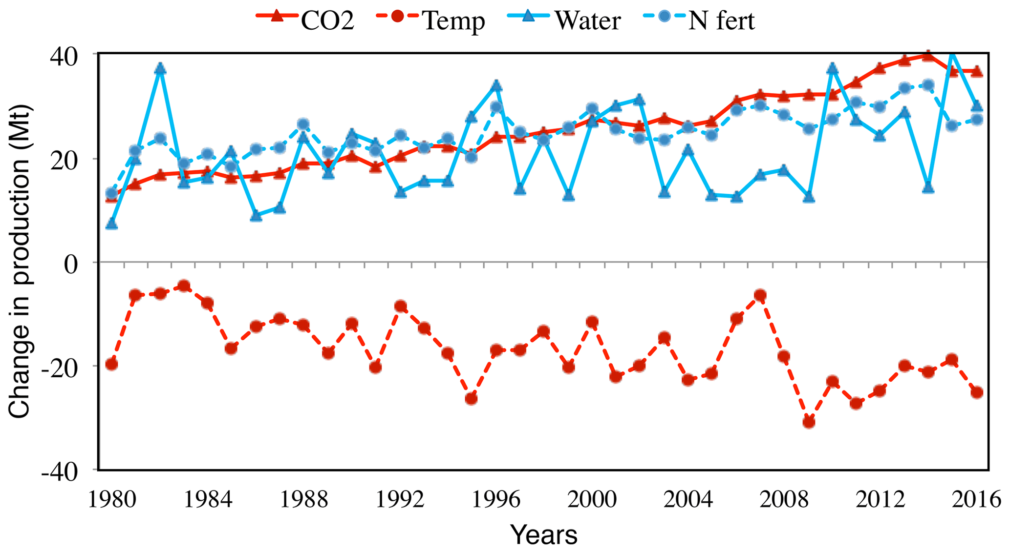
Figure 5 Impact (S_CON–$S_{<\mathrm{factor}>}$) of different environmental factors (atmospheric CO₂ and changing temperature) and land management practices (nitrogen fertilizer and water availability) on production for 1980 to 2016.

Table 3 Temporal variations of different input forcings and their impacts on annual wheat production in India during the study period (1980–2016).

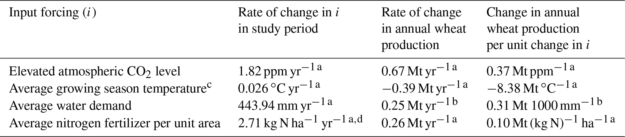
^a Trends are significant at p<0.01. ^b Trends are significant at p<0.1. ^c October to March. ^d Data available from 1980 to 2005.

CO₂ fertilization is the most dominant factor that has contributed to the increase in wheat production in India. Annual average [CO₂] worldwide has increased from 337.7 ppm in 1980 to 404.3 ppm in 2016. This increase in levels of [CO₂] at the rate of 1.82 ppm yr⁻¹ has promoted growth in wheat as elevated [CO₂] levels are known to enhance photosynthetic CO₂ fixation and have a positive impact on most C₃ plants (Myers et al. 2017; Leakey et al., 2009; Allen et al., 1996). Our results show that for every part per million rise in the [CO₂] level the total wheat production of the country has increased by 0.37 Mt (Fig. 6a; Table 3). This amounts to a 22 Mt (30 %) increase in production compared to the 1980–1984 period due to increased [CO₂] levels. A positive correlation coefficient of 0.97 between annual wheat production and annual CO₂ concentration confirms a positive impact of [CO₂] on wheat production. Other studies based on multiple approaches including experiments have also shown an increase in yield and growth of C₃ crops under high [CO₂] conditions (Dubey et al., 2015; Leakey et al., 2009).

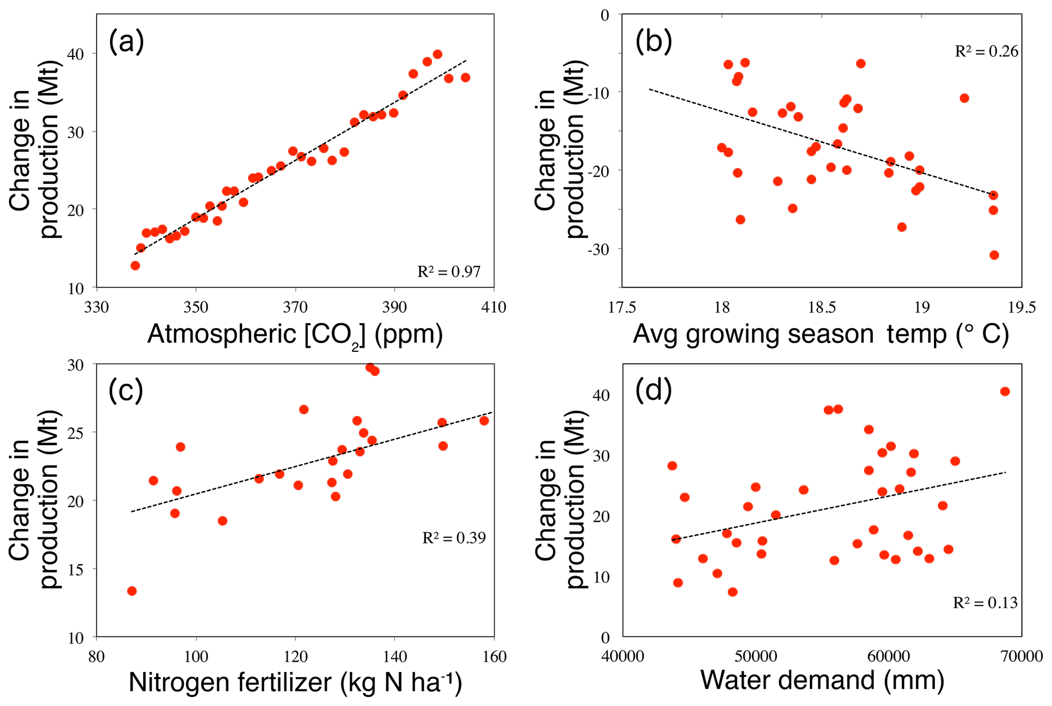
Figure 6 Plots of change in annual wheat production from 1980 to 2016 (S_CON–$S_{<\mathrm{factor}>}$) with annual (a) atmospheric CO₂, (b) average growing season temperature, (c) average nitrogen fertilizer, and (d) water demand. The black line shows Sen's slope (Sen, 1968).

Nitrogen fertilizers are added to the farmland to reduce nutrient stress on the crop. The use of nitrogen fertilizers is important in the Indian context due to two reasons. First, India is a tropical country where higher temperatures and precipitation cause the loss of nitrogen from the soil due to denitrification. Second, crop nitrogen demand is high because multiple cropping is widely practised. The average amount of nitrogen fertilizer added per unit area shows a positive trend of 2.71 kg N ha⁻¹ yr⁻¹ during 1980–2016. This implies an increase in total wheat production at the rate of 0.10 Mt for every kilogram of nitrogen per hectare added to the farm (Fig. 6c; Table 3). This amounts to an 10.63 Mt (15 %) increase in production compared to the 1980–1984 period due to increased fertilizer application.

Irrigation is a key factor for spring wheat in India where 93.6 % of the wheat area is equipped for irrigation (MAFW, 2017), and most of the irrigated area is concentrated in the Indo-Gangetic Plain. Unfortunately, data on the actual amount of water used for irrigation water are not available. Hence, in the S_CON simulation, we consider every grid cell is 100 % irrigated so that the crops do not undergo water stress at any point in the growing season. This is to say that irrigation water required in the model is dependent on the water demand of the crop. With this condition, our results show that with all the regions 100 % irrigated, wheat production shows a positive trend during 1980–2016. Overall, there is a 8.47 Mt (12 %) increase in production compared to the 1980–1984 period due to increased irrigation.

The average air temperature for the months of the wheat growing season (October–March) during the study period (1980 to 2016) showed an increase at the rate of 0.026 ^∘C yr⁻¹. Higher temperatures during the second half of the growing season is specifically known to produce smaller grains and low grain numbers (Stratonovitch and Semenov, 2015; Deryng et al., 2014). Our results have shown a decrease of 8.38 Mt (∼ 10 % reduction) of wheat per degree Celsius increase in average growing season temperature (Fig. 6b). This is higher than the global estimate of 6 % reduction per degree Celsius rise in mean temperature (Asseng et al., 2015). Studies have reported that wheat-growing regions at low latitudes are more susceptible to rising temperatures (Tack et al., 2017; Rosenzweig et al., 2014) since optimum temperatures in these regions have already been reached. Overall, there is a 13 Mt (18 %) reduction in production compared to the 1980–1984 period due to the rise in average growing season temperatures.

In the presence of all input forcings (S_CON), the trend of wheat production in India remains positive at 1.17 Mt yr⁻¹ from 1980 to 2016.

3.3 Effect of environmental and anthropogenic forcings at the regional scale

It is clear that environmental and management factors significantly affect wheat production at a country scale. It is important to understand how these factors can affect production for different regions. For this purpose, the results of the control simulation (S_CON) with all the forcings are analysed for each of the SWEs shown in Fig. 2. A SWE is representative of similar climatic and environmental conditions regionally under which wheat is grown. One SWE differs from the other in terms of different temperature ranges, precipitation received, and irrigation availability. The S_CON case is analysed to ensure that the input factors are fully implemented in the model-estimated production, and their effect can be studied effectively. One important thing to note is that irrigation in the model is calculated as the excess water demand required by the crop to grow in no-water-stress conditions. Hence, the S_CON calculates irrigation as the ideal case scenario assuming that all the water demand of the crop is met. Overall, this analysis will identify the factors (environmental conditions and land management practices) that predominantly drive the wheat production range in a given SWE.

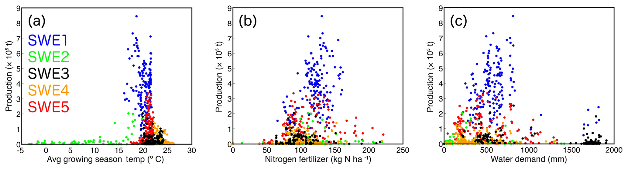
Figure 7 Scatter plots of grid-specific average wheat production from 1980 to 2016 with temporal average of input forcings: (a) growing season temperature, (b) nitrogen fertilizer, and (c) water demand for different SWEs.

The results of this regional analysis are presented in Fig. 7, which shows scatterplots of production as a function of various drivers for each wheat-growing grid cell in the model. A similar plot showing the relationship between production, AEI, and wheat area is presented in Fig. 8. Together, these two figures allow us to understand how different environmental factors and management practices can affect production in different SWEs. Atmospheric [CO₂] is omitted from this analysis because it is assumed to be spatially uniform.

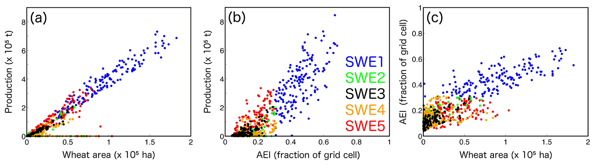
Figure 8 Scatter plots for gridded wheat production with the wheat area and area equipped for irrigation (AEI) for different SWEs.

The Indo-Gangetic Plain region (SWE1) is the best-suited environment for growing spring wheat in India due to favourable growing season temperatures (Fig. 7a), moderate to high fertilizer application (Fig. 7b), high availability of irrigation facilities (Fig. 8b), and moderate water demand (Fig. 7c). Hence, SWE1 is the major contributor to the annual total wheat production of India. Low temperatures (Fig. 7a) in the Himalayan foothill region (SWE2) result in the limited production of wheat in this region. High rainfall in growing season months is helpful, and, hence, limited amounts of water are required for irrigation (Fig. 7c) in this area. The arid north-western Indian region (SWE3) is very low in production due to the high temperatures (Fig. 7a) coupled with a lack of irrigation facilities (Fig. 8b) needed to mitigate the high water demand created by low precipitation. SWE4 in central and north-eastern India is also low in production due to high temperatures during the growing season (Fig. 7a) even though the water demand is low (Fig. 7c) due to moderate rainfall. SWE5 areas in south-central India have limited wheat production because of limited irrigation facilities (Fig. 8b) despite favourable temperature conditions.

Wheat production is directly proportional to the area on which wheat is cultivated in a given region or SWE (Fig. 8a). Figure 8b shows that wheat production is, in fact, positively correlated to AEI at the grid level. Since production in this analysis is derived from the S_CON case and no AEI data are used in its calculation, it is interesting to see such a strong correlation between wheat production and AEI at grid level because they are two independent datasets. This can be explained by Fig. 8c that clearly indicates that availability of irrigation (high AEI) is a major factor that drives the area on which wheat is cultivated in a grid cell. Wheat, being a non-monsoon crop, is highly dependent on the availability of irrigation in a region. For regions with high growing season temperatures, additional water stress is induced in the crop along with heat stress that limits crop production. Hence, the availability of favourable temperatures is crucial for ideal growing conditions for wheat. If irrigation can be made available in these regions, like in SWE5, the wheat cultivation area and wheat production can significantly grow in the years to come.

Table 4 Impacts of different external forcings on annual wheat production in the SWEs during the study period (1980–2016).

^a Values are significant at 99 %. ^b Values are significant at 90 %. ^c October to March.

Similar to the analysis done for the country-scale impact of different factors, we quantified the impact of factors on different SWEs. The results of this analysis are summarized in Table 4. SWE1 and SWE5 are the two regions where the magnitude of trends in the change in wheat production with different input forcings are the highest (Table 4). The magnitudes of the impacts of forcings on SWEs 2, 3, and 4 are relatively small. This is because the analysis involves production that is calculated as the yield times the harvested area. The numbers in Table 4, hence, do not reflect changes per unit of harvested area.

While CO₂ fertilization, water added through irrigation, and nitrogen fertilizers are found to increase wheat production in SWE1 at 0.26 Mt ppm⁻¹ [CO₂], 0.35 Mt (1000 mm)⁻¹, and 0.07 Mt (kg N)⁻¹ ha⁻¹, respectively, production is found to decrease by 3.52 Mt for every degree Celsius rise in average growing season temperatures. It is found that water added through irrigation has a small yet negative impact on production in SWE2. This can be due to excess surface runoff in SWE2 that might lead to the washing away of nitrogen from the soil resulting in nutrient stress in the crop. The impact of different forcings is also found to be significant for SWE5, where [CO₂], irrigation, and nitrogen fertilizers have promoted wheat production at the rates of 0.07 Mt ppm⁻¹ [CO₂], 0.41 Mt (1000 mm)⁻¹, and 0.01 Mt (kg N)⁻¹ ha⁻¹, respectively. Irrigation is seen to have the most impact on wheat production in SWE5 out of all the SWEs.

4 Conclusions and discussions

This study explores the effects of environmental drivers and management practices on spring wheat in India using ISAM. For this purpose, we build and implement a dynamic spring wheat module in ISAM where (i) we parameterize and calibrate the equations in the C₃ crop model framework available in ISAM, (ii) develop new equations for dynamic planting time and heat stress, (iii) collect field data to calibrate and evaluate the model at site scale, and (iv) develop gridded datasets of wheat cultivated area, irrigation, and nitrogen fertilizer data to conduct country-scale simulations. The model is able to simulate the spatio-temporal pattern of spring wheat production at the country scale. This evaluation implies that the model can serve as a simulation tool to conduct numerical experiments to understand the behaviour of spring wheat.

In order to quantitatively study the role of environmental and anthropogenic factors, we conducted a series of numerical experiments by switching off one factor at a time. Our analysis focuses on the 1980–2016 period. Results show that the increase in [CO₂] has a positive impact on wheat production due to the CO₂ fertilization effect. Atmospheric CO₂ concentration has increased by 1.82 ppm yr⁻¹, and production has increased at a rate of 0.37 Mt for every part per million rise in [CO₂] since the 1980s, which translates into a 22 Mt (30 %) increase in countrywide production during the study period. This is consistent with observational studies such as Kimball (2016) that show an increase in yield of C₃ grain crops due to elevated [CO₂].

The application of nitrogen fertilizer has increased at a rate of 2.71 kg N ha⁻¹ yr⁻¹, leading to increased production of spring wheat at the rate of 0.10 Mt for every kilogram of nitrogen per hectare added, which is equivalent to a 10.63 Mt (15 %) increase in countrywide production during the study period. Nitrogen deficiency is very high in India because of high consumption due to multiple cropping and nitrogen loss due to the denitrification of the soil aggravated by the tropical climate. Nitrogen fertilizer contributes to increased production by mitigating this nutrient deficiency.

Our model results suggest irrigation increase could have led to an increase in production of spring wheat at a rate of 0.31 Mt (1000 mm)⁻¹ of water added, implying a 8.47 Mt (12 %) increase in countrywide production during the study period. Irrigation appears to be the most important factor controlling production across all the spring wheat environments. We note here that in our experiments irrigation is equivalent to “no water stress”. This approach seems to be the best option because data on actual water use in irrigation are not available. In grid cells that are equipped for irrigation, we set the water stress term to zero. In reality, water stress may not go to zero in some areas where water or power availability is limited. In these areas, the model underestimates the simulated effect of irrigation on productivity.

Average growing season temperatures have increased by 0.026 ^∘C yr⁻¹ leading to a productivity loss of 8.38 Mt (∼ 10 %) per degree Celsius rise in temperature, which is equivalent to a 13 Mt (18 %) decrease in countrywide production during the study period. Crop heat stress is a major reason behind this loss. The optimum temperature for wheat is 25 ^∘C in the reproductive stage. The heat stress effect is triggered in the model when the canopy air temperature higher than 25 ^∘C and less than 35 ^∘C reduces grain filling and negatively impacts the growth of storage organs. The observed 10 % reduction rate in production is higher than the global average of 6 % (Asseng et al., 2015) because the growing season temperatures in India are already near the upper limit of the optimal range.

The regional-scale analysis shows that SWE1 is the best environment for growing spring wheat in India due to favourable growing season temperatures, moderate water demand, and the availability of irrigation facilities. Hence, this region is the main contributor to the annual total wheat production of India. North-western India (SWE3), covering the states of Rajasthan and Gujarat, is the least productive region due to high growing season temperatures coupled with a lack of irrigation facilities needed to mitigate the high water demand created by low precipitation. Studies have concluded that in order to improve and represent crop growth processes in the models and to increase certainty in model-based assessments, there is a need for more focused regional-scale studies (Maiorano et al., 2017; Koehler et al., 2013). This study is an attempt to work in a similar direction with a focus on wheat in India.

Apart from advancing our understanding of spring wheat growth processes, the crop model can also contribute to real-world decision-making. For example, our results show that wheat production in India has steadily increased at a rate of 1.17 Mt yr⁻¹ from 1980 to 2016. This implies that the negative effect of rising temperatures was offset by positive contributions from other drivers. Our model can be used to conduct experiments to identify optimal solutions to future scenarios. Furthermore, using crop-specific models like the spring wheat model developed in this study will improve the simulation of crop phenology for agroecosystems. This will likely lead to better estimates of carbon fluxes and their spatio-temporal variability.

The Earth system is a non-linear system in which different components interact with each other. In this study, we used a process-based model that includes such interactions and feedbacks between different drivers. For instance, higher temperatures increase the crop water demand. Higher [CO₂] increases photosynthesis that also affects nutrient and water demand. Because of these interactions, the sum of the effects will not add up to 100 %. Moreover, the experiments conducted in this study are not exhaustive; there are other factors like relative humidity and solar radiation that might affect production.

There is scope for improving the crop model and the modelling framework. The processes involved in CO₂ fertilization need improvement to match the Free-Air CO₂ Enrichment (FACE) studies. The addition of new processes accounting for the effects of pests and multiple cropping will make the simulations more representative of the Indian situation. Better data will also improve the fidelity of the simulations. A key bottleneck in simulating crop growth at regional to global scales is the lack of irrigation water use datasets. To the best of our knowledge, large-scale observation-based datasets of water used in irrigation do not exist even though there are numerous datasets for irrigated areas and areas equipped for irrigation (e.g. Zohaib et al., 2019). The development of irrigation water use datasets will reduce the uncertainty in simulating the effect of water stress on crop production. Equipped with these improvements, ISAM can become an indispensable tool for informing policy on food security and climate change adaptation.