the Creative Commons Attribution 4.0 License.
the Creative Commons Attribution 4.0 License.
 | 14 Jul 2020
Reaching 1.5 and 2.0 °C global surface temperature targets using stratospheric aerosol geoengineering
Douglas G. MacMartin
Jan T. M. Lenaerts
Leo van Kampenhout
Laura Muntjewerf
Cheryl S. Harrison
Kristen M. Krumhardt
Michael J. Mills
Ben Kravitz
Alan Robock
A new set of stratospheric aerosol geoengineering (SAG) model experiments has been performed with Community Earth System Model version 2 (CESM2) with the Whole Atmosphere Community Climate Model (WACCM6) that are based on the Coupled Model Intercomparison Project phase 6 (CMIP6) overshoot scenario (SSP5-34-OS) as a baseline scenario to limit global warming to 1.5 or 2.0 ∘C above 1850–1900 conditions. The overshoot scenario allows us to applying a peak-shaving scenario that reduces the needed duration and amount of SAG application compared to a high forcing scenario. In addition, a feedback algorithm identifies the needed amount of sulfur dioxide injections in the stratosphere at four pre-defined latitudes, 30∘ N, 15∘ N, 15∘ S, and 30∘ S, to reach three surface temperature targets: global mean temperature, and interhemispheric and pole-to-Equator temperature gradients. These targets further help to reduce side effects, including overcooling in the tropics, warming of high latitudes, and large shifts in precipitation patterns. These experiments are therefore relevant for investigating the impacts on society and ecosystems. Comparisons to SAG simulations based on a high emission pathway baseline scenario (SSP5-85) are also performed to investigate the dependency of impacts using different injection amounts to offset surface warming by SAG. We find that changes from present-day conditions around 2020 in some variables depend strongly on the defined temperature target (1.5 ∘C vs. 2.0 ∘C). These include surface air temperature and related impacts, the Atlantic Meridional Overturning Circulation, which impacts ocean net primary productivity, and changes in ice sheet surface mass balance, which impacts sea level rise. Others, including global precipitation changes and the recovery of the Antarctic ozone hole, depend strongly on the amount of SAG application. Furthermore, land net primary productivity as well as ocean acidification depend mostly on the global atmospheric CO2 concentration and therefore the baseline scenario. Multi-model comparisons of experiments that include strong mitigation and carbon dioxide removal with some SAG application are proposed to assess the robustness of impacts on societies and ecosystems.
- Article
(13520 KB) - Full-text XML
- BibTeX
- EndNote


Large-scale mitigation efforts to phase out anthropogenic emissions are likely no longer sufficient to keep global mean surface temperature from rising less than 2 ∘C above pre-industrial levels, which is required to avoid significant impacts on societies and ecosystems (IPCC, 2018). Stratospheric aerosol geoengineering (SAG) has been suggested as part of a portfolio of responses, including mitigation, adaptation, and carbon dioxide removal, to potentially reach required surface temperature targets and to reduce some of the effects of anthropogenic interference in the climate system (e.g., Long and Shepherd, 2014; Lawrence et al., 2018; MacMartin et al., 2018). Here, we present climate model experiments designed to assess impacts as a function of future greenhouse gas (GHG) concentrations, the amount of SAG application, target temperatures, and the details of the application.
Various uniformly defined SAG modeling experiments of different complexity have been designed within the Geoengineering Model Intercomparison Project (GeoMIP) to be performed by different modeling groups within phase 5 of the Coupled Model Intercomparison Project (CMIP5) (Kravitz et al., 2011) and CMIP6 (Kravitz et al., 2015). These simulations involve either injecting sulfur dioxide at the Equator or using earlier derived prescribed aerosol distributions to reach the described goals (e.g., Pitari et al., 2014). These were designed, for instance, to keep the radiative forcing at 2020 levels, or apply a constant injection followed by a termination of the injection after 50 years. New GeoMIP experiments were designed for CMIP6, using a high forcing SSP5-85 scenario as a baseline and applying either sulfur dioxide injections or solar dimming in order to reach the moderate radiative forcing of the SSP2-45 scenario (Kravitz et al., 2015). However, no tier 1 GeoMIP experiments have been designed so far to achieve the 2.0 and 1.5 ∘C required temperature targets of the Paris Agreement. Furthermore, earlier GeoMIP experiments specify injections at or in a region around the Equator, which result in excessive cooling of the tropics and less cooling of high latitudes, in turn causing large-scale precipitation shifts (Kravitz et al., 2013).
The Geoengineering Large Ensemble (GLENS) project has defined experiments that aim to keep surface temperature values at close to present-day levels to reduce impacts from global warming (Tilmes et al., 2018). The experiments used a feedback controller to maintain global average surface temperatures, as well as Equator-to-pole and interhemispheric temperature gradients, at 2020 levels. After each year of the simulation, the amount of sulfur injections at each of the four different latitude locations in the stratosphere was calculated, based on the deviations in meeting these surface temperature goals (see the Appendix for more details). GLENS was based on a high forcing future climate scenario (Representative Concentration Pathway 8.5; RCP8.5) and required an increasing amount of sulfur injection with time. GLENS simulations have shown that using global surface temperature and surface temperature gradients, instead of only controlling for global surface temperature, results in reduced side effects, including more even cooling and reduced shifts in precipitation patterns (Kravitz et al., 2019). However, there are other changes in the climate system that do not directly correlate with these quantities. Those include changes in atmospheric circulation and transport, monsoonal rainfall, and chemistry, as well as some responses of the biosphere on land and ocean. The magnitude of changes has been shown to be at least in part dependent on the applied amount and details of the application of SAG (Kravitz et al., 2017, 2019; Richter et al., 2018; Simpson et al., 2019; MacMartin et al., 2019). Furthermore, risks to climate and ecosystems posed by a sudden SAG termination grow with increasing amount of sulfur injection. Consequently, side effects and risks depend strongly on the required amount of intervention application, which is defined by the desired targets and the underlying greenhouse gas concentration pathway.
Several studies have pointed out that SAG may be able to reduce some of the effects of global warming temporarily while decarbonization efforts (including mitigation and negative emissions through carbon dioxide removal) are ramped up. This would be possible if following an overshoot scenario, where mitigation and decarbonization are applied in a way that surface temperatures would peak above desired temperature targets for a limited time and then slowly decline below these temperature targets. A so-called peak-shaving scenario was proposed that would potentially help prevent reaching tipping points until greenhouse gas levels have been sufficiently reduced (Wigley, 2006; Tilmes et al., 2016; MacMartin et al., 2018; Lawrence et al., 2018). Tilmes et al. (2016) and Jones et al. (2018) have produced simulations that kept surface temperature increases to 1.5 or 2 ∘C levels using different RCP forcing scenarios. Jones et al. (2018) used the RCP2.6 scenario as a baseline, resulting in a slight reduction of temperature by the end of the 21st century. Their scenario therefore did not require continuously increasing injections around the Equator but led to some injection reductions by the end of the century to reach 1.5 ∘C temperature targets. Tilmes et al. (2016) used a late decarbonization pathway, starting in 2040 from the high forcing scenario (RCP8.5) and applied different amounts of stratospheric aerosol geoengineering to keep surface temperatures to 2.0 and 1.5 ∘C, using a prescribed aerosol distribution scaled to produce the required cooling. Neither Jones et al. (2018) nor Tilmes et al. (2016) used a feedback algorithm or the multiple injection locations in their approach, as was done in GLENS, and their results showed continued warming in high latitudes and precipitation shifts, while reaching global temperature targets.
The experiments performed here combine two main objectives that have only been addressed separately in previous studies. First, we apply a feedback controller to maintain three temperature targets, in order to reduce some of the side effects identified in earlier studies. Second, we use an overshoot scenario as the baseline scenario to limit the needed amount and duration of SAG to reach a 2.0 or 1.5 ∘C surface temperature target. Furthermore, we use well-defined CMIP6 experiments as baseline experiments that have been performed by various modeling groups. To facilitate baseline scenarios that allow similar peak-shaving geoengineering experiments, as described by Tilmes et al. (2016), CMIP6 designed the overshoot scenario (OS) SSP5-34-OS (O'Neill et al., 2016). This scenario follows the high forcing scenario SSP5-85 until 2040 and then applies drastic decarbonization efforts, including mitigation and active carbon dioxide removal to produce net-negative emissions after 2070. The SSP5-34-OS scenario applies a sudden change in behavior in the consumption of fossil fuel emissions and also assumes large amounts of carbon removal. This produces a carbon dioxide (CO2) concentration overshoot and a surface temperature profile that significantly overshoots the required temperature target before 2100.
We use the state-of-the-art Community Earth System Model version 2 (CESM2) with the Whole Atmosphere Community Climate Model (WACCM6) atmospheric component, from here on called WACCM6, which has been used for CMIP6 simulations. Section 2 describes the model as well as the experiments. We further establish a protocol for new GeoMIP experiments that are designed to reach 1.5 and 2.0 ∘C surface temperature targets and are based on the SSP5-34-OS scenario in order to require less sulfur injection than using a high forcing scenario. We require the use of four pre-defined stratospheric injection locations as well as the use of a feedback controller (or a similar approach) to keep global surface temperatures, interhemispheric and pole-to-Equator surface temperatures, at the defined target temperatures. These experiments are more relevant for impact analysis than any of the existing GeoMIP experiments. We hope to motivate other modeling groups to conduct the same experiments, thereby allowing for an analysis of the outcomes from a multi-model perspective.
We further contrast differences that arise if applying SAG to a high forcing future scenario to reach the 1.5 ∘C temperature target. Resulting sulfur injections, stratospheric sulfur burden, and comparisons of the efficiency using different scenarios are done in Sect. 3. The outcomes of these simulations are discussed in Sect. 4, where we summarize large-scale effects of SAG on surface temperature and precipitation, sea surface temperatures, and the Atlantic Meridional Overturning Circulation (AMOC). In addition, we include some diagnostics that are important for ecosystem and societal impact studies including changes in land primary productivity and land ice mass balance, effects on ocean ecosystems, and the recovery of the Antarctic ozone hole. We do not discuss any detailed regional outcomes based on a two-member ensemble and a single model. Some comparisons are performed with the GLENS project to identify potential ranges of outcomes using an earlier CESM model version. Discussions and conclusions are presented in Sect. 5.
2.1 Model description
The model experiments described here were performed with the WACCM6. Details on CESM2 and WACCM6 model configurations, including an overview of the performance and new features, are described by Danabasoglu et al. (2019) and Gettelman et al. (2019), respectively. The WACCM6 atmospheric model uses a horizontal resolution of 1.25∘ in longitude and 0.95∘ in latitude, and 70 vertical layers, reaching up to 150 km height above sea level ( hPa). Stratospheric dynamics perform well compared to observations, producing an interactive quasi-biennial oscillation (Gettelman et al., 2019). The simulations are performed with comprehensive tropospheric, stratospheric, mesospheric, and lower thermospheric chemistry (Emmons et al., 2019) and an updated secondary organic aerosol scheme in the troposphere (Tilmes et al., 2019). It further uses a modal aerosol scheme (MAM4) for both troposphere and stratosphere (Liu et al., 2016) and prognostic sulfur injection to simulate eruptive volcanoes during the historical period (Mills et al., 2016, 2017). The atmospheric model is coupled to the other components in CESM2. The Parallel Ocean Program version 2 (Smith et al., 2010; Danabasoglu et al., 2012) includes several improvements compared to earlier versions, including ocean biogeochemistry represented by the Marine Biogeochemistry Library, which incorporates the Biogeochemical Elemental Cycle ocean biogeochemistry–ecosystem model (e.g., Moore et al., 2014; Harrison et al., 2018) and the NOAA WaveWatch III ocean surface wave prediction model (Tolman, 2009). Additional components are the sea-ice model CICE version 5.1.2 (Hunke et al., 2015) and the Community Ice Sheet Model version 2.1 (Lipscomb et al., 2019). The Community Land Model version 5 also includes various updates, including interactive crops and irrigation for the land (Lawrence et al., 2019), and the Model for Scale Adaptive River Transport.
CESM2 and WACCM6 have contributed to the Coupled Model Intercomparison Project phase 6 (CMIP6) (Eyring et al., 2016). As part of CMIP6, WACCM6 performed the Diagnostic, Evaluation and Characterization of Klima (DECK) simulations, as well as the historical simulations, which reproduced the observed surface temperature trend within the expected variability (Gettelman et al., 2019).
2.2 Description of the experiments
The SSP5-34-OS CMIP6 scenario is used as the baseline scenario for the GeoMIP testbed experiments. It starts in 2015 from a historical simulation and ends in 2100 (O'Neill et al., 2016). Anthropogenic, biomass burning, ocean, soil, and volcanic emissions are prescribed, as well as surface concentrations of greenhouse gases and land surface values, using the corresponding scenarios (Meinshausen et al., 2017), while biogenic emissions are interactively calculated. SSP5-34-OS follows the same specifications as the SSP5-85 high forcing scenario until 2040. After 2040, the SSP5-34-OS scenario diverts from SSP5-85. SSP5-85 CO2 concentrations continuously increase after 2040 until the end of the 21st century, reaching up to 1100 ppm, and methane (CH4) concentrations increase until 2070 and slowly decline thereafter (Fig. 1b). For SSP5-34-OS, strong mitigation efforts are set in place after 2040, as well as the inclusion of negative emissions. Nevertheless, CO2 concentrations still grow until about 2060, reaching ≈550 ppm, and then slowly decline by the end of the 21st century, reaching ≈500 ppm based on WACCM6 simulations. CH4 concentrations drop relatively quickly after 2040, due to its much shorter lifetime than CO2, reaching values of 1 ppb by the end of the 21st century. This is assuming a drastic phase-out of any anthropogenic production of CH4 after 2040.
Figure 1(a) Annual surface air temperature evolution for two ensemble members of the business-as-usual case (SSP5-85), the overshoot case that is following the SSP-85 case until 2040 and then starting strong mitigation and carbon dioxide removal (SSP5-34-OS), and for three different SAG scenarios: based on the SSP5-85 baseline scenario and applying sulfur injections to reduce warming to 1.5 ∘C above pre-industrial (PI) conditions (Geo SSP5-85 1.5); based on the SSP5-34-OS and reducing warming to 1.5 ∘C above PI (Geo SSP5-34-OS 1.5), and based on the SSP5-34-OS and reducing warming to 2.0 ∘C above PI (Geo SSP5-34-OS 2.0) A 10-year running mean has been applied to all the time series. Black lines indicate the 1850–1900 temperature average (pre-industrial (PI) control temperatures) and the 1.5 and 2.0 ∘C surface air temperatures above PI control. (b) Concentrations of carbon dioxide (CO2, dotted lines) and methane (CH4, solid line) for the two baseline simulations.
Two climate intervention experiments are designed to use the same prescribed greenhouse gas concentrations, emissions, and land surface values as the baseline SSP5-34-OS scenario. The experiments are designed to maintain global mean near-surface temperatures around 1.5 and 2.0 ∘C warming compared to 1850–1900 levels, respectively, and are called “Geo SSP5-34-OS 1.5” and “Geo SSP5-34-OS 2.0”. The start of each climate intervention experiment is defined by the time that the baseline simulation has reached a near-surface global mean temperature of 1.5 and 2.0 ∘C above pre-industrial, considering a 10-year running mean (in WACCM6, this is around 2020–2025 for 1.5 ∘C and around 2034 for 2 ∘C). For easier comparisons, all ensemble members use the same exact numbers for reaching the three temperature targets, even if surface temperatures slightly vary for different ensemble members.
Besides global mean surface temperature targets, we require two more surface temperature measures in the proposed experiments, namely interhemispheric temperature gradients and Equator-to-pole temperature targets, as described in Kravitz et al. (2016) and MacMartin et al. (2017). These additional temperature targets are defined based on the period when global mean surface temperatures have reached the specific climate goals; see above. Sulfur dioxide injections into the stratosphere are performed at four locations 5 km above the tropopause, at 15∘ N, 15∘ S, 30∘ N, and 30∘ S in latitude, and at an arbitrary longitude of 180∘ W, following the approach described in Kravitz et al. (2017) and Tilmes et al. (2018). We suggest the use of a feedback control algorithm, as applied here, that was developed by MacMartin et al. (2017), based on an earlier WACCM version 5.4 (WACCM5.4) (Mills et al., 2017). The injection rate each year is computed based on an initial guess (a “feedforward”) that is corrected based on the actual temperature history (the “feedback”). The feedforward function helps the controller more easily to reach the goals. This algorithm has been adopted in the WACCM6 without any changes, despite using a slightly different scenario in WACCM6 (using SSP5-85) compared to GLENS (using RCP8.5). For the OS simulations, the same feedback algorithm was applied but with changes to the feedforward function to account for the different temperature evolution in the baseline simulation. Details are described in the Appendix.
In this study, two realizations of the proposed experiments have been performed. Since the SSP5-85 scenario is identical to SSP5-34-OS until 2040, we started the SSP5-34-OS in 2040 from the SSP5-85 scenario. WACCM6 near-surface temperatures reached around 1.3 ∘C warming compared to the 1850–1900 average by 2015 and 1.5 ∘C around 2020–2025 using the two WACCM6 ensemble members from the historical simulation (Fig. 1a). The global mean surface warming reaches 6.3 ∘C by 2100. The SSP5-34-OS global mean surface temperature reaches up to 3 ∘C above the 1850–1900 temperature by 2060, aligned with the maximum peak in CO2 concentrations. Temperatures slightly decline by the end of the century to about 2.5 ∘C above pre-industrial. Global near-surface temperature targets were reached in the two SAG model experiments within about 0.2 ∘C (Fig. 1a, green and orange lines).
In addition to the proposed GeoMIP testbed experiments, we also performed a third climate intervention experiment that uses SSP5-85 as the baseline scenario, while applying sulfur injections to keep near-surface temperature levels at 1.5 ∘C targets, called “Geo SSP5-85 1.5”. This scenario is identical to the “Geo SSP5-34-OS 1.5” experiment between 2015 and 2040 (Fig. 1a, purple lines). This experiment is not required for the proposed GeoMIP testbed experiment but can be useful for additional analysis. Comparing the outcomes of Geo SSP5-85 1.5 with the Geo SSP5-34-OS 1.5 experiment allows us to explore the differences of the impact of SAG using a high forcing greenhouse gas scenario vs. the overshoot scenario after 2040. Geo SSP5-85 1.5 can also be compared to the results in GLENS, since it uses the same setup with a similar baseline simulation but different model versions (WACCM5.4). GLENS simulations include a three-member ensemble of the future baseline simulation starting in 2010, following the RCP8.5 pathway, called “RCP8.5” in the following. GLENS SAG simulations reached the same surface temperature targets of around 1.5 ∘C and are called “Geo RCP8.5 1.5” in the following (see Table 1).
Table 1Overview of model simulations.
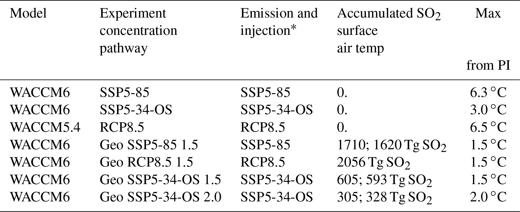
* Ensemble mean for GLENS (Geo RCP8.5 1.5); the two numbers correspond to the two ensemble members for the WACCM6 Geo cases.
The feedback algorithm calculates the required injection amount per injection location after each year of the simulation, based on the surface temperature deviations from the target temperatures. For all of the cases, a larger fraction of the injection was placed into the Southern Hemisphere (SH) (Fig. 2). For Geo SSP5-85 1.5, the injections were mainly placed at 30∘ N and 30∘ S, with a slightly smaller amount in the Northern Hemisphere (NH). Only half of the amount that was used at 30∘ S was required at 15∘ S and almost no injection was required at 15∘ N to achieve the pre-defined temperature goals. For the Geo SSP5-34-OS 1.5 and Geo SSP5-34-OS 2.0 experiments, most injections were placed at 30∘ N, 30∘ S, and 15∘ S. After 2080, for Geo SSP5-34-OS 1.5 (2070 for Geo SSP5-34-OS 2.0), only injections in the SH were needed, and injections at 15∘ S dominated. As a result, the sulfate loading is significantly larger over the SH than the NH. This is in contrast to what has been simulated in Geo RCP8.5 1.5 (GLENS), where more injections were required in the NH in order to achieve the same temperature targets (Tilmes et al., 2018). An in-depth investigation is needed in future studies to understand the differences using the two different CESM model versions. However, differences may be in part connected to differences in the ocean response, described in Sect. 4, and may be a result of differences in anthropogenic sulfur emissions between SSP5-85 and RCP8.5.
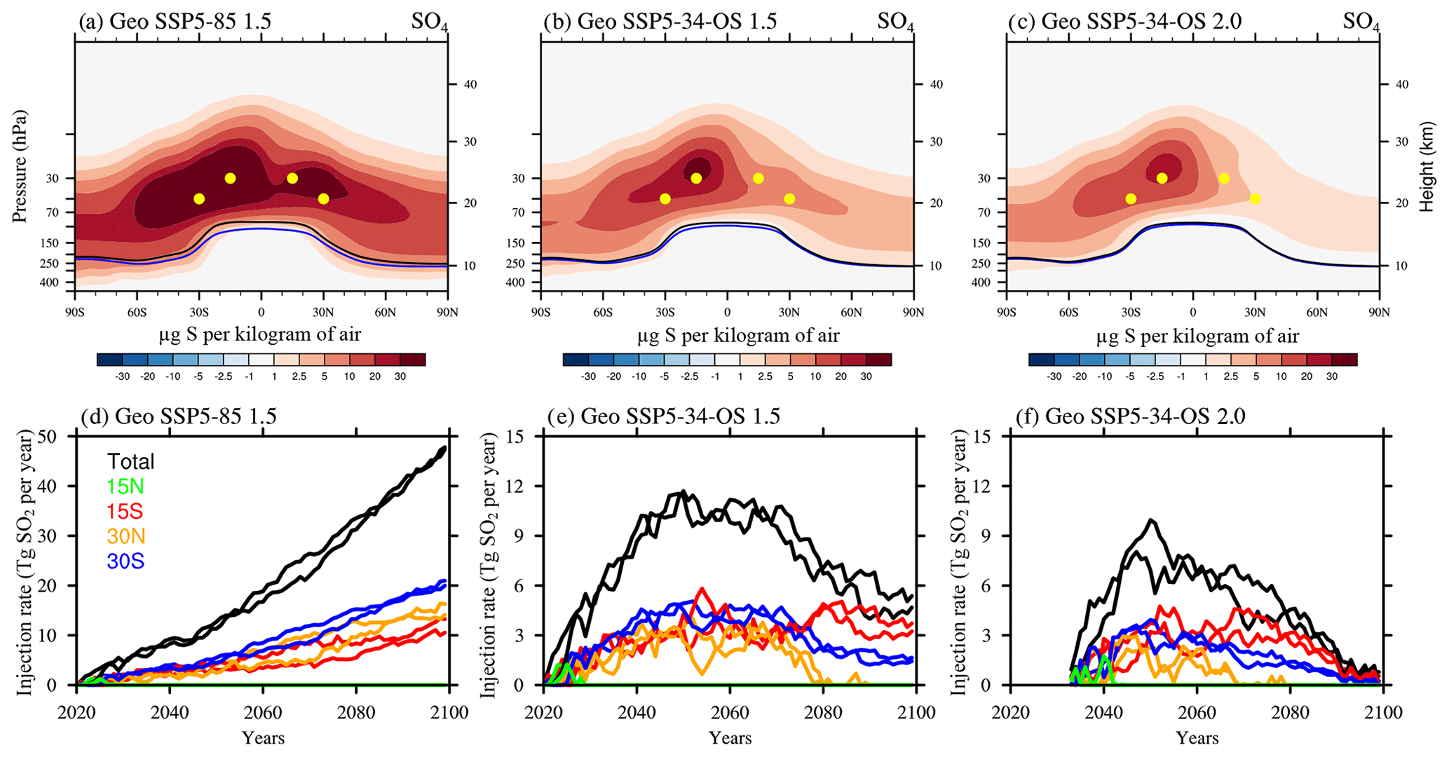
Figure 2(a–c) Difference of zonally and annually averaged sulfate SO4 burden between the ensemble average of stratospheric sulfur injection cases in 2070–2089 and the control experiment for the same period for Geo SSP5-85 (a), Geo SSP5-34-OS 1.5 (b), and Geo SSP5-35-OS 2.0 (c). The lapse rate tropopause is indicated as a black line for the control and a blue line for the SO2 injection cases. Yellow dots indicate locations of injection. (d–f) Injection rate in Tg SO2 per year for the three cases as in panels (a–c) (including two ensemble members): total injections (black), injections at 15∘ N (green), 15∘ S (red), 30∘ N (orange), and 30∘ S (blue).
Differences between the three SAG experiments and the Geo RCP8.5 1.5 also arise in terms of accumulated SO2 injection amount (Table 1) and aerosol burden with regard to sulfur injections per year (Fig. 3). The maximum injection amount in Geo SSP5-85 1.5 is 48 Tg SO2 per year with a total burden reaching up to 25 Tg S. This results in an accumulated injection amount of 1710 and 1620 Tg SO2, respectively, for the two ensemble members by the end of the century (Table 1). In contrast, Geo RCP8.5 1.5 required a larger injection with an accumulated injection amount of 2056 Tg SO2 and a corresponding burden of 28 Tg S. The correlation between sulfur burden and injection rate is similar between Geo RCP8.5 1.5 and Geo SSP5-85 1.5 (Fig. 3b), which concludes that production, transport, and removal processes in the two WACCM versions are similar. The reason for the slightly smaller required injection amount in Geo SSP5-85 1.5 compared to Geo RCP8.5 1.5 could be due to differences in the baseline scenarios, which specify a larger sulfate burden in the troposphere in SSP5-85 compared to RCP8.5 (not shown).

Figure 3Annual averaged stratospheric sulfate aerosol burden in Tg S for the geoengineering injection experiments minus the control with time (a) and injection rate (b). The stratospheric burden vs. injection amount (in units of years) is listed in the bottom panel for the two ensemble members of each experiment. In addition to the model experiments performed in this study, we add results for GLENS. See text more details.
The two SAG experiments that are based on the OS scenario show much reduced accumulated SO2 injections compared to the high forcing scenarios, with 605 and 593 Tg SO2 for the 1.5 ∘C temperature target and 305 and 328 Tg SO2 for the 2.0 ∘C temperature target for each of the two ensemble members. For Geo SSP5-34-OS 1.5, the total annual injection peaks between 2050 and 2070 at 10–12 Tg SO2, an amount comparable to the observed global sulfate perturbation from the 1991 eruption of Mt. Pinatubo (Baran and Foot, 1994; Dhomse et al., 2014; Mills et al., 2016). For Geo SSP5-34-OS 2.0, injections peak around 2050, reaching between 7 and 9 Tg SO2, and fall off after that towards around 1 Tg SO2 injections per year by the end of the century. In particular for the OS cases, there were periods in which the near-surface temperatures were slightly cooler than the target temperature. This was likely due to shortcomings in the feedforward component of the controller setup; in particular, the feedforward was estimated based only on the instantaneous cooling required and did not adequately take into account the “memory” in both the aerosol concentrations and the resulting temperature response. The feedforward component thus overestimated the amount of SO2 injection required once aggressive mitigation began; this was eventually successfully corrected by the feedback. Both experiments that are based on the OS baseline scenario show a larger burden per injection amount (Fig. 3b) for the years when SO2 injections have been declining because of the prevalent sulfate burden from previous years.
4.1 Surface air temperature changes
The design of the proposed testbed experiments allows us to assess the effects of SAG, while surface air temperatures are maintained at specific targets, here 1.5 and 2.0 ∘C above pre-industrial levels. Since 1.5 ∘C of warming, the more desired temperature target defined by the IPCC1.5 report, is reached around 2020 (2015–2025) for the first ensemble member of the WACCM6 SSP5-85 simulation, we use this period as the control period for our analysis. Results in Figs. 4 and 5 are therefore illustrated in reference to 2015–2025 control values based on SSP5-85. The evolution of global mean surface air temperatures in the different experiments has been described above. Here, we discuss the surface air temperature evolution in NH and SH, in order to illustrate interhemispheric temperature differences (Fig. 4, solid and dotted lines, respectively) for the different experiments.
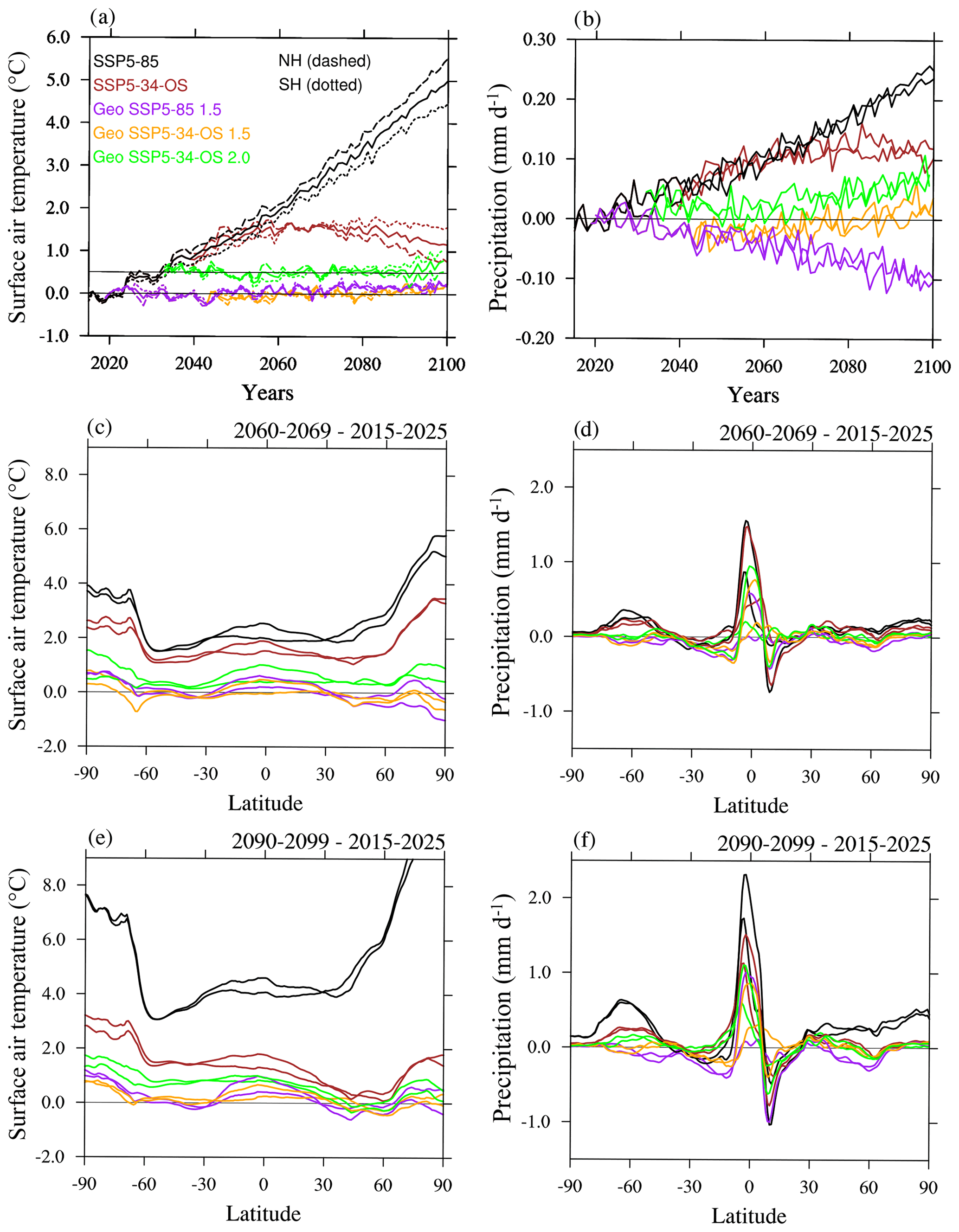
Figure 4(a) Time evolution of the ensemble mean area-weighted annual mean surface air temperature with regard to 2010–2025 conditions, averaged over the globe (solid), over the Northern Hemisphere (dashed), and over the Southern Hemisphere (dotted) for different model experiments (different colors; see legend); (b) time evolution of area-weighted annual precipitation with regard to 2015–2025 conditions for different model experiments and ensemble members (different colors); differences of zonal mean surface air temperatures (c, e) and precipitation (d, f) with regard to 2015–2025 SSP5-85 conditions for values in 2060–2069 (c, d) and 2090–2099 (e, f) for the different model experiments (different colors).
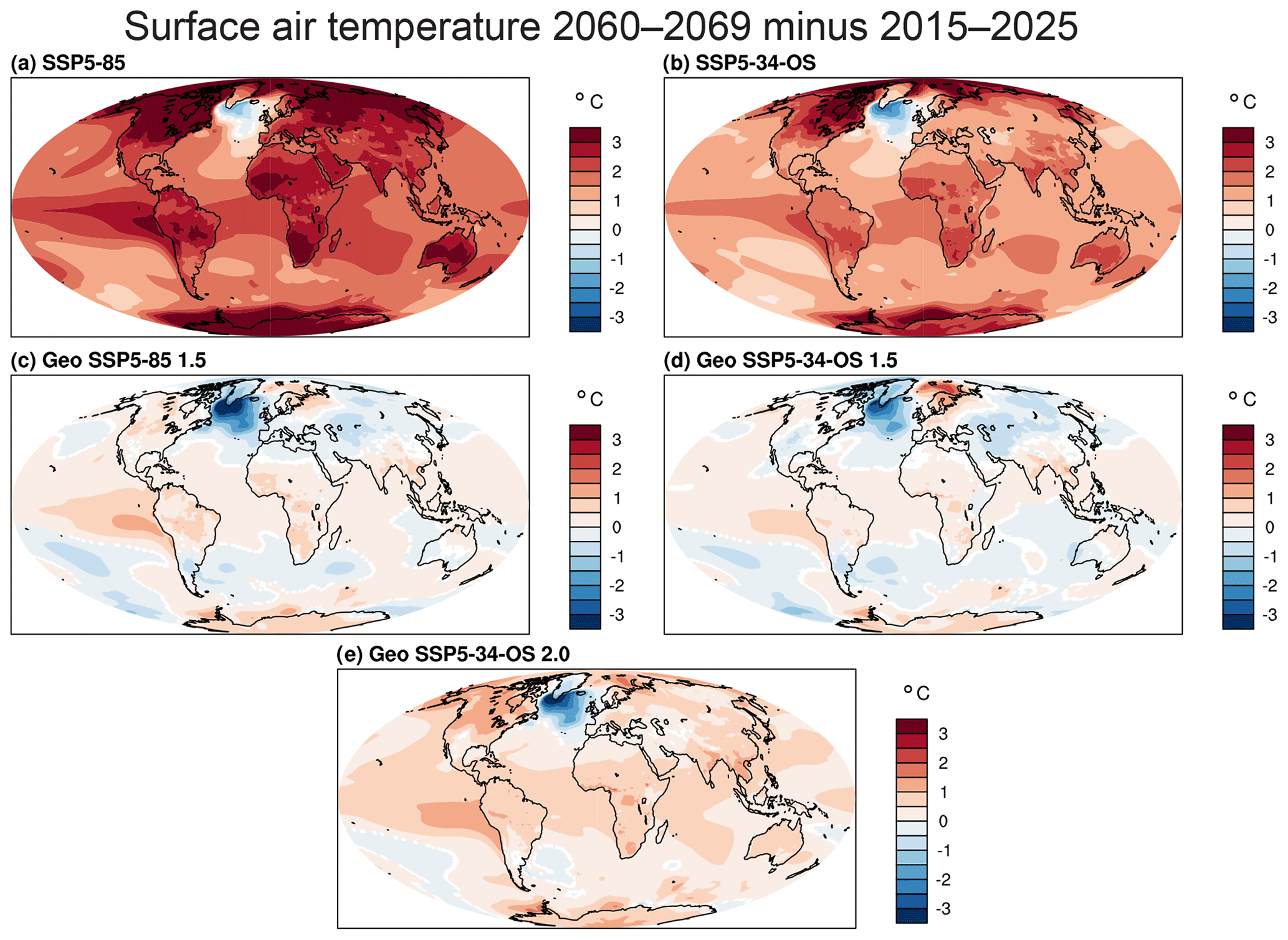
Figure 5Ensemble-mean surface air temperature difference between 2060–2069 and 2015–2025 for SSP5-85 and SSP5-35-OS (a, b), Geo SSP5-85 1.5 and Geo SSP5-34-OS 1.5 (c, d), and Geo SSP5-35-OS 2.0 (e). Regions shaded in color are significant with 95 % confidence based on Student's t test.
The two baseline simulations (SSP5-85 and SSP5-34-OS) show an increase in deviations of hemispheric surface air temperatures from the global mean temperature. While in SSP5-85, interhemispheric temperature differences continue to increase towards the end of the 21st century with stronger temperature trends in the NH compared to the SH, interhemispheric temperature differences in SSP5-34-OS reverse around 2070. This results in very small temperature trends in the SH after 2070 and decreasing temperatures in the NH. In WACCM6, NH temperatures are strongly impacted by the so-called “warming hole” in the North Atlantic, which describes a local cooling that counters increasing temperatures from increasing greenhouse gas concentrations (Fig. 5a and b). The cooling of surface air temperatures above the North Atlantic is similar in magnitude for both SSP5-85 and SSP5-34-OS, likely a result of a fairly similar slowdown of the AMOC, as discussed in Sect. 4.2. On the other hand, the warming in the NH due to increasing greenhouse gas concentrations is much larger in SSP5-85 than in SSP5-34-OS, resulting in the differences in north-to-south temperatures between the two baseline scenarios.
Applying the feedback algorithm to SSP5-85 and SSP5-34-OS results in a removal of the interhemispheric gradient in addition to maintaining global mean surface air temperatures. Only the last 15 years (2085–2100) of the Geo SSP5-34-OS 2.0 experiment produce somewhat larger warming in the SH than in the NH (Fig. 4a, c, e). Zonal mean surface air temperature changes from the different experiments are illustrated for two different periods in Fig. 4c and e. For the baseline simulations, temperature anomalies in high latitudes are higher than in midlatitudes and low latitudes, as expected, leading to much larger warming than the global mean. Effects of the warming hole (cooling) in the North Atlantic are visible (Fig. 5), particularly for the SSP5-34-OS scenario towards the end of the 21st century. SAG applications show a significant reduction in the warming of the polar regions, with very little difference between pole and Equator in all the sulfur injection experiments. Only a slight warming up to 1 ∘C occurs in the SH polar region by the end of the 21st century. The continuous cooling in the North Atlantic (Fig. 5c and d) is compensated by a warming over northwest Europe. Temperature goals are therefore reached equally well in all the sulfur injection experiments, using different baseline scenarios. The Geo SSP5-34-OS 2.0 scenario is slightly cooler in the NH and shows a slight warming in the SH compared to the temperature target. This experiment is designed to be 0.5 ∘C warmer than the other two SAG experiments. Therefore, independent of reaching the 1.5 or 2.0 ∘C temperature targets, the feedback approach is able to maintain zonally averaged surface air temperatures at most latitudes.
4.2 Atlantic Meridional Overturning Circulation changes
Sea surface temperature (SST) anomalies are significantly reduced by SAG in all scenarios. Simulated present-day (2015–2025) SST is already significantly warmer than pre-industrial (PI) across the tropics, subtropics, and into the Southern Ocean, with anomalies between 0.5 and 1.5 ∘C, reaching 2 ∘C in the equatorial Pacific for one ensemble member (Fig. A2). On top of this, in the 2060s, simulated SST is significantly warmer than 2015–2025, with broad regions reaching anomalies above 2 ∘C in the SSP5-85 case and 1.5 ∘C in the SSP5-34-OS case; the exception is the warming hole in the North Atlantic (Drijfhout et al., 2012), which is significantly and persistently cooler by 1–2 ∘C from both PI and present-day SST by 2070, even in SSP5-85 (Fig. A3). SST anomalies are largely reduced in all geoengineering protocols implemented in this study, especially in the 1.5 ∘C cases, with the exception of the warming hole, which remains persistently cool in all scenarios. Regions of persistently warm anomalies remain in the 2.0 ∘C case, including much of the eastern Indian Ocean and the equatorial eastern South Atlantic based on the two ensemble members.
The apparent warming hole in all of the simulations is very likely related to changes in the AMOC (Fig. 6). The baseline scenarios SSP5-85 and SSP5-34-OS show a very similar decline until the last two decades of the simulation, with a maximum decline of more than 50 % by the end of the century. Both SAG scenarios that target the 1.5 ∘C temperatures show only a relatively small decline from 2020 values (approximately 25 %), with the largest reduction during the last 20 years of the simulation. The Geo SSP5-34-OS 2.0 produces a stronger decline closer to 40 % and therefore closer to the SSP5-34-OS baseline scenario.
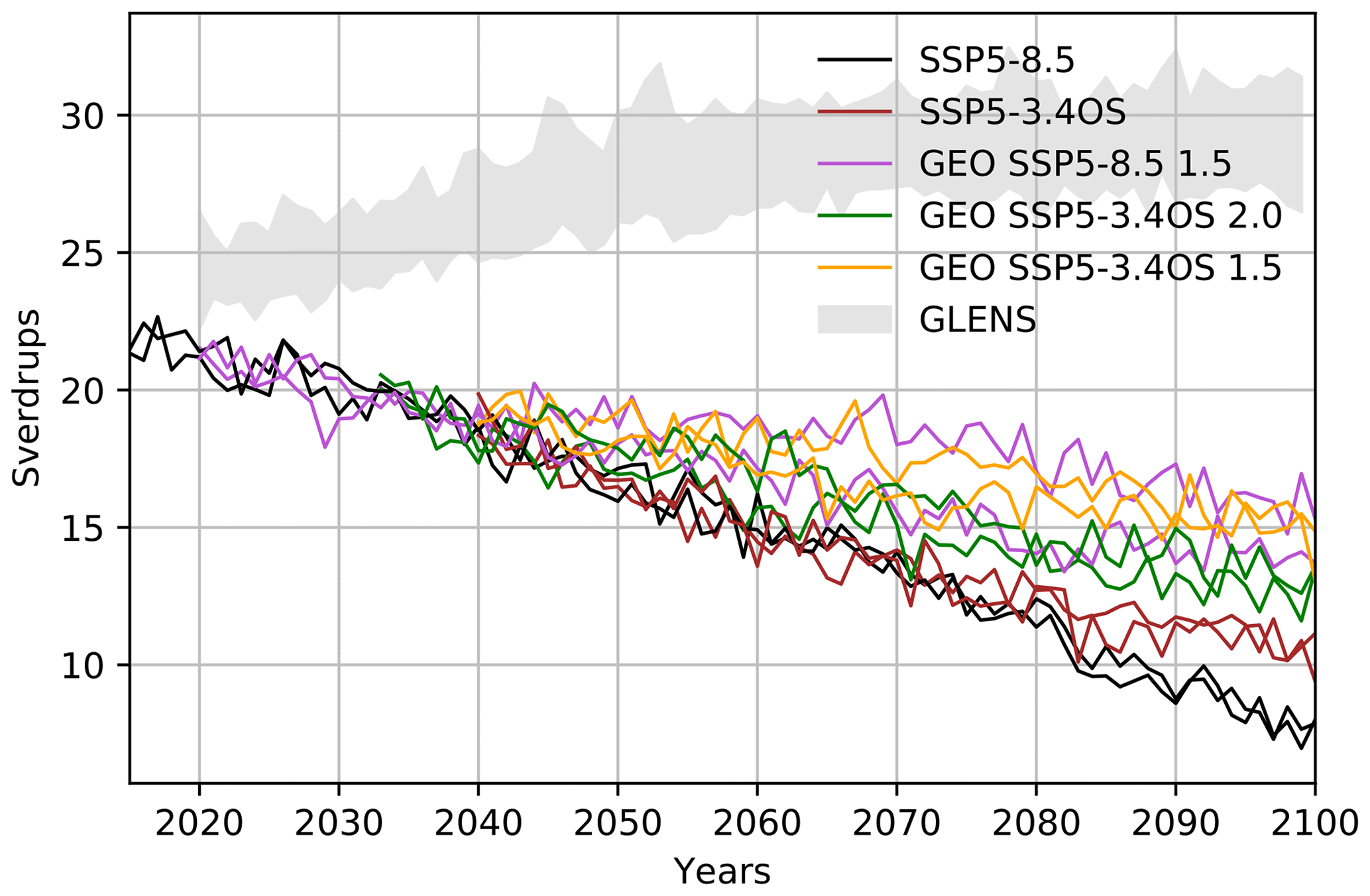
Figure 6Evolution of the maximum North Atlantic Meridional Overturning Circulation strength from the AMOC index for the different scenarios and ensemble members. Shaded grey area is AMOC index range in the 21-member GLENS ensemble. The AMOC index is defined as the maximum flux in the Atlantic basin between 500 m depth to the bottom, and between 28 and 90∘ N (Sverdrups).
In comparison, Geo RCP8.5 1.5 (GLENS) simulations do not show the relative cooling in the North Atlantic (Fasullo et al., 2018). The earlier version of the model shows a slowing of the AMOC for the RCP8.5 scenario similar to the WACCM6 CMIP6 SSP5-85 simulation, which is however much smaller. Danabasoglu et al. (2019) found that the maximum AMOC strength in CESM2 is stronger than in CESM1. The differences in AMOC between CESM1 and CESM2 reflect differences in water mass properties that are ascribed (partly) to surface flux differences, as the ocean model component in both model versions handles the dense-water overflows through the Denmark Strait and the Faroe Bank Channel in the same way. Applying SAG resulted in an acceleration of the AMOC in GLENS (Fig. 6, grey shaded area), which is not the case in any of the WACCM6 SAG simulations. In these simulations, the AMOC is still declining, even though less severely than in the SSP5-8.5 simulation. Responses of AMOC and therefore effects on surface air temperatures seem to be largely model version dependent.
4.3 Zonal mean precipitation changes
Global mean precipitation is changing compared to the 2015–2025 control (Fig. 4b), even though global surface air temperatures are maintained using SAG, as expected based on various earlier studies. Similarly to what has been found in Tilmes et al. (2016) and Jones et al. (2018), precipitation is increasing for the baseline scenarios, while applications of a low forcing scenario result in close to present-day global precipitation values. In WACCM6, precipitation is declining the most compared to 2020 values in Geo SSP5-85 1.5, with increasing reductions towards the end of the century, aligned with the increasing amount of sulfur dioxide injections, which is very similar to what has been found in GLENS (e.g., Fasullo et al., 2018). However, the SAG experiment based on the OS pathway and aiming for the 1.5 ∘C target, results in a much smaller global mean precipitation change. Furthermore, Geo SSP5-34-OS 2.0 shows a slight increase in global mean precipitation with increasing values after 2070.
Large-scale precipitation changes from the control are shown in the zonal mean precipitation anomalies (Fig. 4d and f). Both baseline simulations (SSP5-85 and SSP5-34-OS) show increasing precipitation in tropics and midlatitudes to high latitudes between 2060 and 2069. While this trend continues in SSP5-85, the SSP5-34-OS shows a reduction in the precipitation changes compared to control, as a result of reduced warming in this scenario by the end of the 21st century. A shift in tropical precipitation towards the SH (and therefore a shift in the Intertropical Convergence Zone – ITCZ) occurs and is most pronounced in the SSP5-85, with increasing intensity towards the end of the 21st century in both baseline scenarios. Despite the reduction in greenhouse gases and surface temperature relative to SSP5-85, impacts on tropical precipitation using the overshoot scenario are still large and may result in large regional impacts. SAG applications successfully reduce increasing precipitation and shifts in tropical precipitation in 2060–2069, with slight reductions in precipitation in the SH subtropics. Some larger differences occur by the end of the 21st century, where reductions in precipitation are most pronounced if using the SSP5-85 baseline scenario. Also, the strength in the shifts in tropical precipitation differs within the different ensemble members. More detailed investigations have to be performed in future studies, as well as in a multi-model comparison context. Precipitation changes are therefore strongly dependent on the amount and strategy of SAG application.
4.4 Land primary productivity
Net primary productivity (NPP) over land is the difference between gross primary productivity (GPP) and plant respiration (Cramer et al., 1999), and it is a key component in the terrestrial carbon cycle. NPP is sensitive to climate changes, including temperature, precipitation, soil moisture and photosynthetically active radiation. As shown in previous analysis (Cheng et al., 2019), relative to the baseline, SAG would reduce temperature, change precipitation and evaporation, which would potentially change soil moisture, and reduce the total incoming solar radiation. Therefore, terrestrial NPP is influenced by SAG.
Figure 7 shows the accumulated annual land NPP in different baselines and SAG scenarios. The shaded areas around the curves illustrate the natural variability of NPP based on pre-industrial control conditions. Differences between the scenarios are considered to be significant if they lie outside the shaded area, as is the case for SSP5-85 and Geo SSP5-85 1.5, showing a slight reduction in NPP if SAG has been applied. The other scenarios do not show a significant difference. NPP shows strong dependency on CO2 concentration, consistent with previous studies (Govindasamy, 2002; Kravitz et al., 2013; Glienke et al., 2015). In CLM5, CO2 concentration is one of the factors to determine the stomatal resistance and photosynthesis rate (Lawrence et al., 2019). With higher CO2 concentration in SSP5-85 and Geo SSP5-85 1.5, plants tend to have less stomatal conductance, which makes them more resistant to water stress, and to have higher photosynthesis rate. Therefore, land NPP in those two scenarios increases constantly through the whole simulation period. With mitigation and carbon dioxide removal strategy, CO2 concentration under SSP5-34-OS and the related SAG scenarios reaches a maximum around 2060, and then reduces slowly. In general, land NPP in our simulations follows the change of CO2 concentrations in the baseline. Temperature reduction or other climate changes from SAG show mild impact on land-accumulated NPP. However, comparison between baseline and SAG indicates regional different responses of land NPP to SAG climate changes.

Figure 7Annual land-accumulated NPP (Gt C yr−1) in baseline and SAG scenarios and ensemble members (different colors are indicated in legend). The shaded areas are significant with 95 % confidence, assuming normally distributed data.
Figure 8 shows NPP anomalies between the three SAG scenarios and their baseline during 2060–2069. Significance of results is assumed if the difference between the two simulations that are compared is larger than the natural variability, assuming the standard deviation (σ) in each model grid cell of the yearly means from the 499-year pre-industrial control run. An anomaly was considered significant when it was greater than 1.96σ (95 % confidence interval, assuming normally distributed data). There are similar patterns in the maps with SAG, where land NPP increases over tropical and midlatitude regions, while it decreases over high-latitude and high-altitude areas. The temperature reduction from SAG plays an important role in this pattern (Kravitz et al., 2013). Lower leaf temperature over tropical and midlatitude regions enhances stomatal conductance and hence promotes the carbon gain, while over high-latitude and high-altitude regions, the cooling is not optimal for plant growth. The magnitude of changes depends on both baseline and the temperature target. With a larger temperature difference between the baseline and the SAG, the NPP changes are bigger. As shown in Fig. 7, NPP changes are the largest between SSP5-8.5 and Geo SSP5-8.5 1.5.
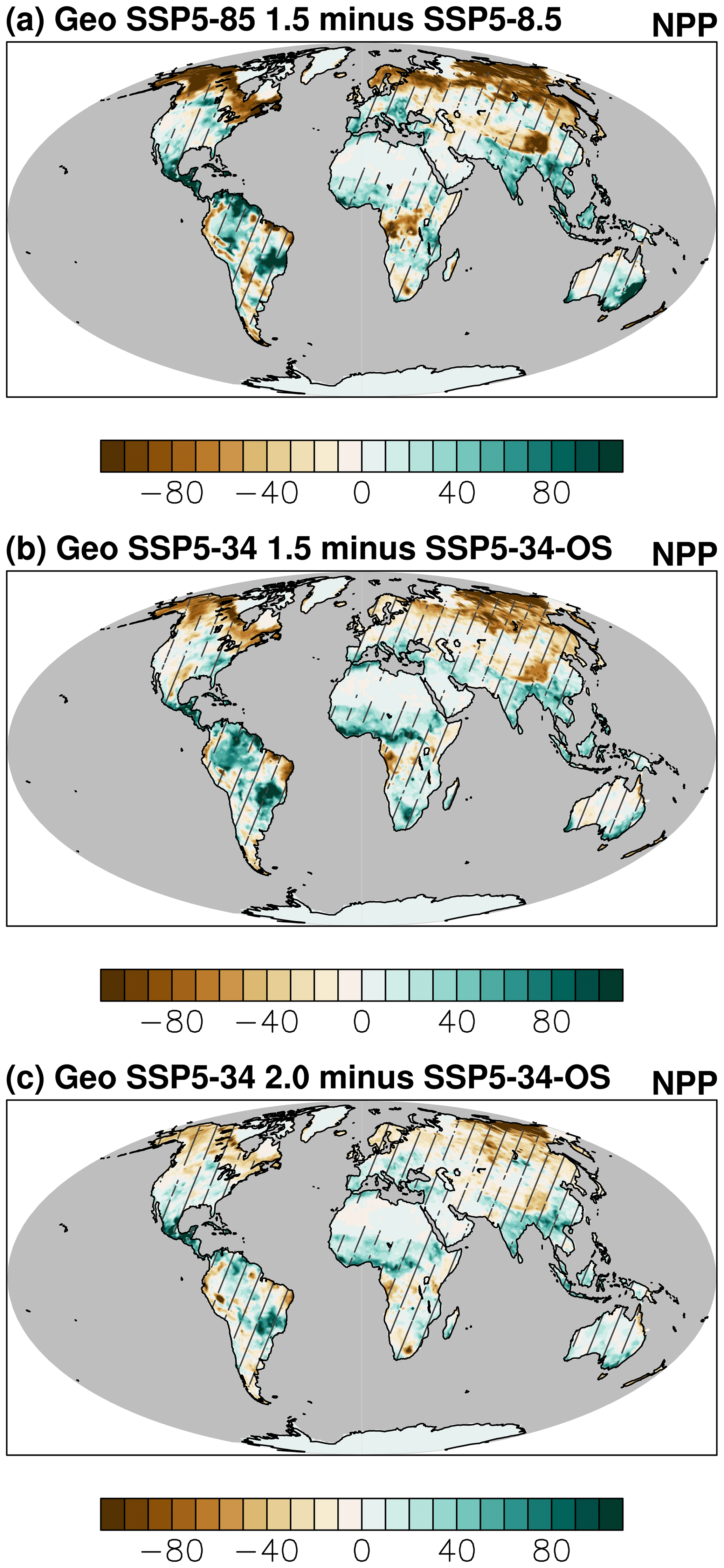
Figure 8Ensemble mean land-accumulated NPP difference (g C m−2 yr−1) between 2060 and 2069 for Geo SSP5-85 1.5 and SSP5-85 (a), Geo SSP5-34-OS 1.5 and SSP5-34-OS (b), and Geo SSP5-34-OS 2.0 and SSP5-34-OS (c). Hatched regions are areas not significant with 95 % confidence, assuming normally distributed data.
4.5 Ocean ecosystem impacts
Warming has large impacts on ocean ecosystems and fisheries, both directly through ocean temperature impacts on physiological processes, and indirectly through warming-induced changes in ocean physics. Increases in ocean temperature elevate respiration rates for endothermic (cold-blooded) animals, including zooplankton and fish, decreasing body size and limiting energy transfer to commercial fishery species and large marine vertebrates (Heneghan et al., 2019; Lotze et al., 2019). In contrast, warming ocean temperatures may stimulate NPP by phytoplankton, marine primary producers that make up the base of the marine food web, assuming no other changing conditions (Eppley, 1972; Krumhardt et al., 2017). Additionally, however, warming drives changes in ocean stratification, currents, and other physical mechanisms (clouds, sea ice, river flow) that affect nutrient delivery processes and available light (Laufkötter et al., 2015; Lauvset et al., 2017; Harrison et al., 2018). For example, warming-induced stratification increases in pelagic ecosystems may reduce the amount of nutrients supplied to the photic zone, decreasing marine NPP, indirectly impacting higher trophic levels. Combined together, net responses of marine ecosystems to climate perturbations are dependent on local physical and biogeochemical conditions, leading to diverse ecosystem responses in different regions (Bopp et al., 2013; Krumhardt et al., 2017; Lauvset et al., 2017). Globally integrated, these processes are predicted to cause a net decrease of globally integrated oceanic biological production in future climate scenarios (Krumhardt et al., 2017), with a projected 5 % decline in fisheries production for every degree of surface temperature warming (Lotze et al., 2019). Here, we investigate to what degree solar radiation management mitigates the primary drivers of marine ecosystem disruption, sea surface temperature, and net primary productivity.
Anomalies outside historical climate variability are one indication of ocean conditions that ecosystems are not adapted to and thus expected to cause disruption to fisheries and natural ecosystems (Bopp et al., 2013; Heneghan et al., 2019). As for land NPP, significance of SST (Fig. A3) and ocean NPP (Fig. 9) anomalies was determined by using the standard deviation (σ) in each model grid cell of the yearly means from the 499-year pre-industrial control run. An anomaly was considered significant when it was greater than 1.96σ (95 % confidence interval, assuming normally distributed data).
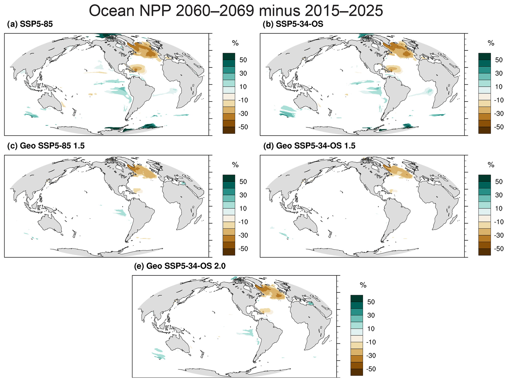
Figure 9Ensemble mean percent difference in ocean net primary productivity (NPP) in 2060–2069 relative to 2015–2025. Regions shaded in color are significant with 95 % confidence, assuming normally distributed data.
Oceanic NPP, the rate of photosynthetic carbon fixation by marine phytoplankton (Krumhardt et al., 2017; Harrison et al., 2018), represents the base of marine food web, supporting fisheries and natural ecosystems and driving the biological carbon pump that removes CO2 from the atmosphere (e.g., Sarmiento and Gruber, 2006; Harrison et al., 2018). Similar to previous Earth system model simulations, anomalies of NPP in future climate are highly variable in space and feature both strong positive and negative anomalies (Fig. 9), driven by different mechanisms in different biomes (Bopp et al., 2013; Krumhardt et al., 2017). In contrast to SST, simulated NPP is not significantly different in 2015–2025 relative to PI over much of the global ocean, with the exception of increased NPP at the poles, where both declining ice and warming temperatures increase production, and a narrow strip at the subtropical–subpolar boundary in the Southern Hemisphere (Fig. A2); these anomalies get stronger by 2070 (Fig. 9). Additionally, the North Atlantic warming hole is associated with NPP declines of 30 %–40 %, likely caused by changes in nutrient supply. All anomalies are substantially mitigated by SAG, with positive NPP anomalies relative to present disappearing over much of polar oceans, and NPP reductions in the North Atlantic decreasing from 30 %–40 % (baseline cases) to 20 %–30 % in the 1.5 ∘C SAG cases. Thus, SAG could reduce negative impacts of climate change on marine ecosystems in the North Atlantic, an important region for fisheries. It is important to note, however, that the ocean ecosystem model in CESM2 does not account for the effects of ocean acidification on marine phytoplankton, which could impact, for example, calcifying phytoplankton (Krumhardt et al., 2019) or diatoms (Bach et al., 2019; Petrou et al., 2019).
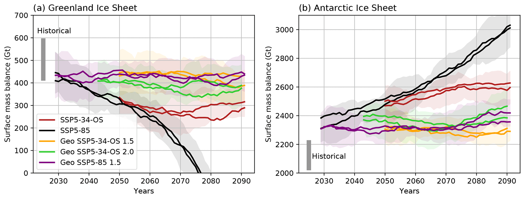
Figure 10Mean ice sheet surface mass balance (SMB) in Gt yr−1. Shading indicates standard deviation of one of the members, calculated after detrending the time series using empirical model decomposition. A 20-year running mean has been applied to filter out year-to-year variability. For the Greenland Ice Sheet (GrIS) (a), the area of integration is the contiguous ice sheet (1 699 077 km2). For the Antarctic Ice Sheet (AIS) (b), the area of integration is the grounded ice sheet (12 028 595 km2). The solid grey bar indicates the ±1 SD (standard deviation) SMB over the period 1960–1999 in CESM2 (WACCM) for reference.
4.6 Ice sheet surface mass balance
The mass balance (MB) of (grounded) ice sheets, which determines their contribution to sea level rise, is made up of two components: the surface mass balance (SMB; representing snowfall and surface melt) and solid ice discharge (D) across the grounding line (Lenaerts et al., 2019).
As D is controlled by ice flow speed and ice thickness, and responds relatively slowly to external forcing, it is challenging to detect an impact from SAG on ice discharge within a single century. Moreover, default CESM2 and therefore WACCM6 does not explicitly represent D, as it requires a dynamic ice sheet model coupled to the ESM, a feature that is currently only available in dedicated CESM2 experiments (Lipscomb et al., 2019). SMB, on the other hand, is explicitly represented in CESM2 (van Kampenhout et al., 2020). Since SMB is primarily driven by atmospheric and surface processes, in particular snowfall and surface melting, it has a much shorter response time than D. In addition, while ice sheet SMB exhibits large interannual variations, it also is observed to show a discernible trend on ice sheets in both hemispheres (Lenaerts et al., 2019). The observed Greenland Ice Sheet mass loss and associated sea level rise is primarily driven by a declining SMB (van den Broeke et al., 2016) and will very likely continue to do so in the future (Aschwanden et al., 2019). A common tipping point for the Greenland Ice Sheet (GrIS) is assumed to be SMB of 0, when the ice sheet no longer has a mechanism to gain mass; this threshold is likely already reached this century in higher-emission scenarios (Pattyn et al., 2018). In contrast, the Antarctic Ice Sheet (AIS) SMB has increased throughout the past century (Medley and Thomas, 2019), potentially acting to mitigate Antarctic mass loss through increasing D. While we are not able to identify the impact of SAG on Antarctic D, recent studies indicate that the Antarctic Ice Sheet will likely become unstable (leading to a sharp increase in D) when we increase global mean temperature by above 2 ∘C (Pattyn et al., 2018).
In Fig 10a, a general decrease in GrIS SMB is seen in all simulations compared to the historical period, but most notably in the high-warming scenarios (SSP5-85 and SSP5-34-OS). This decrease is driven by increased surface runoff (Fig. A4), which is only partly offset by increased snowfall (not shown). SAG is effective in stabilizing runoff and therefore SMB in all three simulations, albeit there still is a distinct departure from late 20th century values. Although this is good news for the stability of the GrIS, and the tipping point SMB of 0 is only reached in SSP5-85, it does not guarantee the GrIS existence in the long run since we do not resolve discharge. Moreover, the SMB–elevation feedback is not explicitly modeled, which starts to play a dominant role on millennial timescales (Pattyn et al., 2018). Based on these results, we deem it unlikely that large freshwater fluxes will originate from the GrIS by surface processes alone in all three geoengineering scenarios.
Figure 10b shows AIS SMB. In contrast to the GrIS, surface runoff plays only a minor role on the AIS (Fig. A4) and the overall trend is dominated by increased snowfall with temperature, resulting in increased SMB. A discernable departure from 1960–1999 values is obvious in all simulations due to end of 20th century warming. Throughout most of the 21st century, the response of AIS SMB is similar in all SAG simulations (Fig. 10b). The early stabilization in these simulations confirms the short response time of SMB, on the order of years to decades. Interestingly, simulations Geo SSP5-34-OS 1.5 and SSP5-85 1.5 depart from one another during the second half of the 21st century. We attribute this difference to the different aerosol loading in the two simulations, which impacts the formation of precipitation.
4.7 Evolution of the Antarctic ozone hole
The annually recurring ozone hole over Antarctica that began around 1980 is a result of enhanced chlorofluorocarbons (CFCs) and other halogen reservoirs in the stratosphere, the so-called ozone-destroying substances (ODSs), that mostly accumulated before the 1990s. Due to the very long lifetime of some CFCs (over 100 years), the burden of ODS peaked around the year 1990 and is now slowly declining. The Antarctic ozone hole is expected to recover back to 1980 values in 2060 (WMO, 2018). However, changes in surface climate due to anthropogenic climate change are projected to accelerate the Brewer–Dobson circulation in the stratosphere and with that transport more ozone into high latitudes and increase ozone with time, which can lead to a “super-recovery” of ozone. The larger the forcing scenario, the larger this effect, which would potentially slightly speed up the recovery of the ozone hole. RCP8.5 simulations as part of GLENS show the recovery of the Antarctic ozone in October by around 2060 compared to 1980 total column ozone values (Fig. 11a) and an increase of column ozone up to 30 DU by the end of the century. The same behavior is also shown in WACCM6 following SSP5-85. Overshoot scenarios also show a recovery to 1980 values, which stays at or slightly below that value for the rest of the simulations, as a result of the reduced climate change effect on ozone (Fig. 11b).
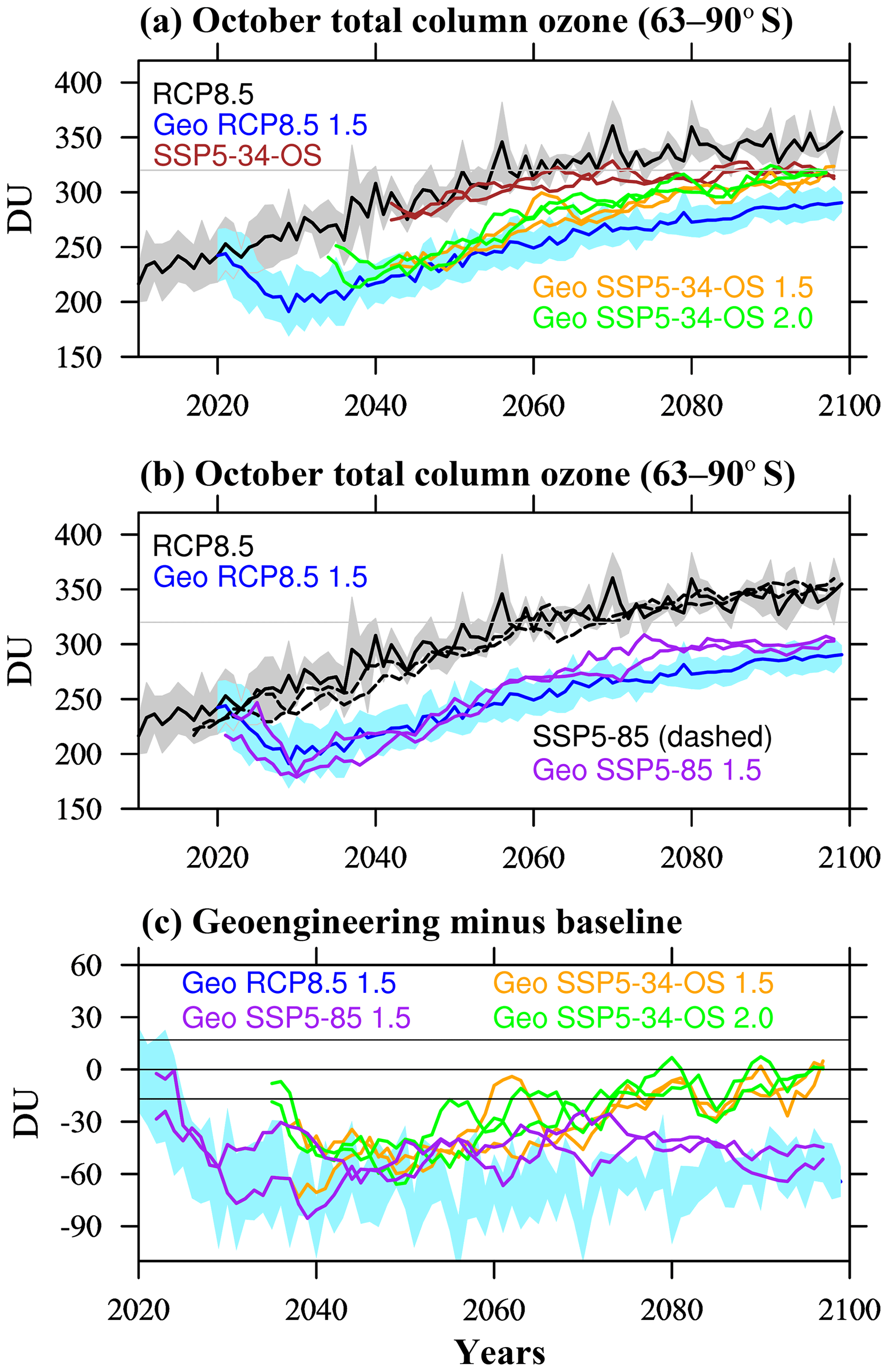
Figure 11October averaged total column ozone between 63 and 90∘ S for different model experiments and ensemble members (different colors) (a, b). Grey and light blue areas show the standard deviation of the GLENS ensemble and the light grey line indicates 1980 values. (c) Differences between geoengineering and corresponding baseline experiments; the two black lines around zero indicate the standard deviation from the GLENS baseline simulations. A running mean over 5 years has been applied to the results.
The increasing aerosol burden in the stratosphere in the SAG modeling experiments has significant effects on stratospheric chemistry and transport (e.g., Tilmes et al., 2009; Ferraro et al., 2014; Richter et al., 2018). The absorption of radiation by sulfate aerosols heats the lower tropical stratosphere. The amount of heating is proportional to the sulfur injection amount and results in a drop of the tropopause altitude and an increase in tropopause temperatures (Tilmes et al., 2017). These changes, in addition to the cooling of the surface and the troposphere, influence the strength of the subtropical and polar jets and therefore transport of stratospheric air masses, which results in changes in ozone. In addition, stratospheric aerosols increase the aerosol surface area important for heterogeneous reactions. This leads to an enhanced activation of chlorine and therefore increased ozone depletion in the polar stratosphere. The effect of SAG was estimated to delay the recovery of the ozone hole by at least 40 years (Tilmes et al., 2008). Changes in stratospheric ozone in regions outside the SH polar latitudes as the result of SAG will be discussed in future studies.
Both GLENS and WACCM6 simulations show a drop in Antarctic column ozone at the start of the SAG application between 2020 and 2030 of up to 70 DU and then an increasing trend, similar to the case without SAG application. Antarctic column ozone has not fully recovered in Geo SSP5-85 1.5 by the end of the century. On the other hand, the SAG scenarios Geo SSP5-34-OS 1.5 and 2.0 show a faster recovery of the ozone hole than Geo SSP5-85 1.5, which is reached around 2080. The reduced forcing scenario does require less sulfur injections to reach the temperature targets, which results in a smaller stratospheric aerosol burden. Therefore, less ozone depletion is expected and the delay of the recovery of the ozone hole would be shortened to 20–30 years. For SSP5-34-OS 2.0, the later start of SAG application leads on average to a weaker reduction of column ozone of around 45 DU compared to the drop in column ozone of around 60 DU if SAG would be started in 2020.
This paper describes a set of new SAG simulations using WACCM6, which aim to keep global warming to less than 1.5 or 2.0 ∘C above pre-industrial. The overshoot scenario SSP5-34-OS has been used as the baseline scenario, which follows the SSP5-85 future pathway until 2040, and then drastically increases decarbonization afterwards. The resulting overshoot in surface temperatures above the desired temperature targets allows the application of a peak-shaving scenario that requires limited SAG applications in time and amount, compared to steadily increasing injections needed for a high forcing scenario. We acknowledge that the SSP5-34-OS scenario is not a recommended scenario, because of delayed actions in mitigation and carbon dioxide removal; however, it is the only CMIP6 scenario that produces a temperature overshoot before the end of this century. More realistic and policy relevant scenarios need to be designed in the future that include earlier actions on mitigation, more realistic implementation of potential negative emissions and assumed surface emissions.
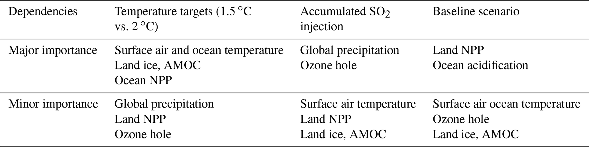
Table 2Impacts dependent on different measures: achieved temperature targets applying SAG, amount of sulfur burden, and the baseline scenario.
In addition to reaching global surface temperature targets, the experiment requires the achievement of interhemispheric and pole-to-Equator temperature targets, which can be done by using a feedback control algorithm to identify annual stratospheric injection amounts at four different latitudinal locations. For example, Kravitz et al. (2017) have shown several improvements in using the feedback controller to achieve the three temperature targets. Reaching global temperature surface targets of 1.5 or 2.0 ∘C and keeping interhemispheric and pole-to-Equator surface temperatures from changing has been shown to reduce global impacts, including heatwaves, sea ice melting, and large shifts in precipitation patterns. This scenario would therefore reduce climate impacts and risks, and therefore provide a complete picture for studying impacts on society and ecosystems as compared to using unrealistic SAG applications based on a high greenhouse gas scenario. However, before impact studies are meaningful, multi-model experiments are required to identify the range of outcomes and uncertainties. We therefore recommend including these experiments as a new testbed GeoMIP scenario for CMIP6.
Here, we further compare the experiments that are based on the OS scenario to SAG applications using the high greenhouse gas emission scenario SSP5-85, and to the earlier performed GLENS simulations that are based on the RCP8.5 scenario. These experiments provide the opportunity to explore the range of outcomes of SAG dependent on the amount of SAG injections, the background CO2 concentrations, and the target surface air temperatures. Applications of the feedback controller to achieve the three temperature targets in WACCM6, global surface temperatures, and interhemispheric and pole-to-Equator temperature gradients, result in small differences in the relative amount of warming in high latitudes between a 1.5 and a 2 ∘C temperature target. Therefore, differences that were described in the IPCC1.5 report (IPCC, 2018) between reaching the 1.5 or 2 ∘C target may be different if they are reached with SAG or with emission reductions only, and have to be investigated further. On the other hand, global precipitation changes depend on the amount of sulfur injections, resulting in a stronger reduction with increasing application. Precipitation changes and shifts in the ITCZ occur in both baseline scenarios and in the OS case by the end of the century. This is likely a result of changes in the distribution of tropospheric aerosols. SAG using the feedback algorithm helps to reduce these shifts, whereby reduction in precipitation is strongest with higher injection amounts and to a lesser amount depends on the temperature targets.
The impacts of SAG need to be explored within the entire space between scenarios and societal and ecological relevant impacts to holistically assess and improve SAG applications. Here, we provide examples of how such an assessment could be established, considering different types of scenarios, e.g., high-GHG scenarios, low-GHG scenarios, high vs. low SAG, and differences in temperature targets. All of these matter for different impact variables in a different manner. There are many different variables that need to be investigated. This paper explores only a few of those variables and illustrates their dependency on impacts based on temperature targets, amount of sulfur burden, and the baseline simulations (Table 2). Furthermore, differences in injection amounts will impact costs of the implementation and need to be considered but have not been investigated here.
Changes in AMOC, that are coupled to the surface temperatures, lead to a significant warming hole in WACCM6 with consequences for ocean temperatures, reducing NPP in the ocean in the North Atlantic. The reduced slowing of the AMOC with SAG would decrease some impacts on marine ecosystems. However, SAG will not mitigate other ecosystem stressors, like ocean acidification, which depend on the baseline scenario. Land NPP is also strongly dependent on the CO2 content of the atmosphere and therefore on the baseline simulations but not so much on the temperature target. On the other hand, mean ice sheet surface mass balance is strongly dependent on the surface temperature target and has only a small direct dependence on the amount of SAG application or the baseline simulations. Finally, the Antarctic ozone hole is expected to recover around 2060 without SAG but cannot fully recover by the end of the century if SAG would be applied to the SSP5-85 baseline scenario to reach 1.5 ∘C. Using the OS scenario, ozone super-recovery is reduced and SAG applications would delay the recovery by approximately 20–30 years until around 2080, with a slightly early recovery if the 2 ∘C target would be used.
In summary, future changes in different quantities that are important for societal and ecological impacts depend on very different measures, including the amount of SAG application, temperature target, and baseline simulation. A comprehensive assessment is required that holistically considers benefits and side effects of climate intervention strategies.
The injection rates necessary to achieve desired temperature targets through stratospheric sulfur injections in Earth system models are strongly model and scenario dependent. A trial-and-error approach could in principle be used to determine, in each model, the necessary injection rates as a function of time. However, this can be time-consuming even with only a single goal and a single latitude of injection, and may be prohibitive for tuning the time-varying injection rates across multiple latitudes to simultaneously meet multiple climate goals, particularly when the unknown injection rates might also depend nonlinearly on the amount of cooling needed. In addition, a simple trial and error approach is not able to respond smoothly to changes, which can however be done with applying control theory. We thus chose to use a trained control algorithm to effectively “learn” the right injection rates to use (MacMartin et al., 2014; Kravitz et al., 2016) and recommend a similar approach if other modeling centers want to repeat these experiments in different models.
A best estimate (also called the feedforward) for the required injection rates is first determined; if this were perfect, then no correction would be needed. A feedback algorithm is then used to update the injection rates after each year of the simulation in response to the error in meeting the goals over the previous years. The approach is documented in detail in Kravitz et al. (2016, 2017). The first step to reach the three temperature targets is to control for aerosol optical depth (AOD), which can then be directly related to the sulfur injections. The algorithm first computes the projection of AOD onto three independent basis functions. Thus, the global mean AOD is adjusted in response to an error in the global mean temperature, the interhemispheric difference in AOD adjusted in response to an error in interhemispheric temperature gradient and Equator-to-pole difference in AOD adjusted in response to Equator-to-pole temperature gradient. The injection rates at each latitude are then determined based on the desired AOD (see also MacMartin et al., 2017). Neither the relationship between injection rates and spatial patterns of AOD, nor the relationship between those patterns of AOD and the resulting surface temperature response need to be known accurately, as the feedback will converge despite uncertainty.
The feedforward provides the feedback control algorithm with an initial estimate on the needed injections. The feedforward that was used in Kravitz et al. (2017) and Tilmes et al. (2018) was a simple linear scaling of the desired cooling, with the proportionality estimated from 10-year simulations described in Tilmes et al. (2017). For the simulations conducted here, the same approach was used. The time-varying amount of cooling relative to the desired target was computed using the baseline simulations and fitted with a simple functional form. The feedforward functions () had to be fit to the different cases as illustrated in Fig. A1 with k being a function of years between the start of the injection and the end of the simulations:
-
SSP5-8.5, 1.5 ∘C target: ;
-
SSP5-34-OS, 1.5 ∘C target: for k<2050, ;
-
SSP5-34-OS, 2 ∘C target: .
Furthermore, because of the memory inherent in the system, more injection is needed while GHG levels are increasing than at the same temperatures later in the overshoot runs while GHG levels are decreasing. Because the feedback algorithm does not correct this error immediately, there is some temporary overcooling in our simulations roughly when the peak GHG warming (peak desired cooling from SAG) is obtained; this could have been corrected by accounting for the system memory in designing the feedforward. For the feedback correction, the same proportional–integral control law as in Kravitz et al. (2017) was used here. Thus, in each year of the simulation, the desired values for each of the three basis functions of AOD are computed as the sum of that year's best-estimate value (the feedforward), and a two-term feedback correction, as
where S (the injection amounts in the next year) is the sum of the best estimate or feedforward value for year k+1, and a feedback correction. Kp and Ki are the proportional and integral control gains, whereby Kp only reacts to the temperature error in the previous year (T[k]). Ki is required to ensure zero steady-state error (the correction in response to the integrated error will continue to build as long as there is nonzero bias in the error). The summation in the integral term begins from the first year of injection (j=0) through to the year of simulation just completed.
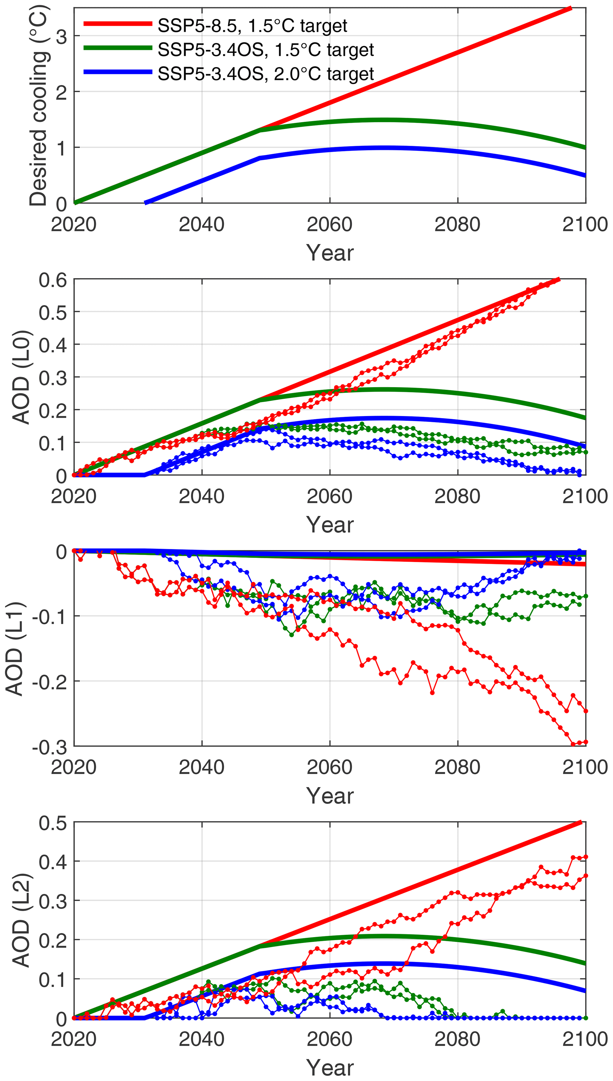
Figure A1Feedforward used in simulations. Top panel shows the fit to the desired temperature reduction for different cases (see text for details). Remaining panels show both the feedforward (best guess for desired AOD prior to conducting the simulation) and actual AOD after feedback correction (dotted lines) for the global mean AOD (L0), the projection of the AOD onto sin(lat) (the interhemispheric gradient L1), and the projection onto a quadratic (the Equator-to-pole gradient L2). There is substantial error in the initial guess, due to a combination of uncertainty, nonlinearity, and making the feedforward in a given year only proportional to the desired temperature reduction in that year; this illustrates the importance of using a feedback algorithm to correct these initial guesses.

Figure A2Simulated sea surface temperature (SST) anomaly (a) and % change in net primary productivity (NPP) (b) in SSP5-8.5 2015–2025 relative to pre-industrial long-term means. Regions shaded in color are significant with 95 % confidence, assuming normally distributed data.

Figure A3Ensemble mean sea surface temperature (SST) in 2060–2069 relative to 2015–2025 for different scenarios (different panels). Regions shaded in color are significant with 95 % confidence, assuming normally distributed data.
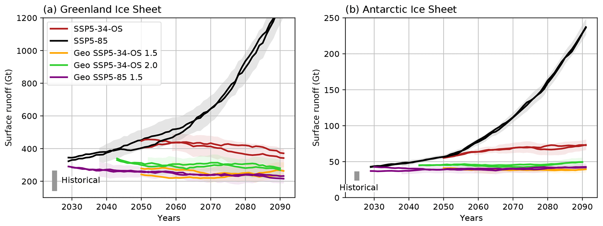
Figure A4Mean ice sheet runoff in Gt yr−1. Shading indicates standard deviation of one of the members, calculated after detrending the time series using empirical model decomposition. A 20-year running mean has been applied to filter out the high year-to-year variability. The area of integration is the same as in Fig. 10. The solid grey bar indicates the ±1 SD (standard deviation) runoff over the period 1960–1999 in CESM2 (WACCM) for reference.
Previous and current CESM versions are freely available (http://www.cesm.ucar.edu:/models/cesm2, last access: July 2020) (NCAR, 2020a). The CESM2 WACCM6 SSP5-85 and SSP5-34-OS data analyzed in this paper have been contributed to CMIP6 and are freely available at the Earth System Grid Federation (ESGF; https://esgf-node.llnl.gov/search/cmip6/, last access: July 2020) (ESGF, 2020) or from the NCAR Digital Asset Services Hub (DASH; https://data.ucar.edu, last access: July 2020) (NCAR, 2020b) or from the links provided from the CESM website (http://www.cesm.ucar.edu/, last access: July 2020) (NCAR, 2020c) under https://doi.org/10.5065/D67H1H0V (Danabasoglu, 2020). The additional SAG experiments are available under https://doi.org/10.26024/t49k-1016 (Tilmes, 2020).
As the first author, ST organized and wrote a large portion of the paper, produced all the simulations, and performed the analysis presented in about half of the figures. DGM was instrumental in properly setting up the feedback algorithm, and contributed to the interpretation of results and the writing of the paper. JTML and LvK analyzed land ice mass balance and produced related figures and text. LM produced AMOC figures and the corresponding text. LX analyzed land primary productivity and produced related figures and text. CSH and KMK analyzed sea surface temperature and ocean net primary productivity, producing related figures and text. MJM, BK, and AR contributed to the writing of the paper and the overall framing.
The authors declare that they have no conflict of interest.
We thank Douglas E. Kinnison and Anne K. Smith for helpful comments and suggestions. This material is based upon work supported by the National Center for Atmospheric Research, which is a major facility sponsored by the NSF under cooperative agreement no. 1852977. Computing and data storage resources, including the Cheyenne supercomputer (https://doi.org/10.5065/D6RX99HX), were provided by the Computational and Information Systems Laboratory (CISL) at NCAR.
This research has been supported by the National Science Foundation (grant no. CBET-1931641), the Indiana University Environmental Resilience Institute, the Prepared for Environmental Change Grand Challenge initiative, the US Department of Energy by Battelle Memorial Institute (grant no. DE-AC05-76RL01830), the NSF (grant nos. AGS-1617844 and 1852977), the Computational and Information Systems Laboratory (CISL) at NCAR, the Netherlands Earth System Science Centre (NESSC), and the Ministry of Education, Culture and Science (OCW) (grant no. 024.002.001).
This paper was edited by Valerio Lucarini and reviewed by two anonymous referees.
Aschwanden, A., Fahnestock, M. A., Truffer, M., Brinkerhoff, D. J., Hock, R., Khroulev, C., Mottram, R., and Khan, S. A.: Contribution of the Greenland Ice Sheet to sea level over the next millennium, Sci. Adv., 5, eaav9396, https://doi.org/10.1126/sciadv.aav9396, 2019. a
Bach, L. T., Hernández-Hernández, N., Taucher, J., Spisla, C., Sforna, C., Riebesell, U., and Arístegui, J.: Effects of elevated CO2 on a natural diatom community in the subtropical NE Atlantic, Front. Mar. Sci., 6, 1–16, https://doi.org/10.3389/fmars.2019.00075, 2019. a
Baran, A. J. and Foot, J. S.: New application of the operational sounder HIRS in determining a climatology of sulphuric acid aerosol from the Pinatubo eruption, J. Geophys. Res., 99, 25673, https://doi.org/10.1029/94JD02044, 1994. a
Bopp, L., Resplandy, L., Orr, J. C., Doney, S. C., Dunne, J. P., Gehlen, M., Halloran, P., Heinze, C., Ilyina, T., Séférian, R., Tjiputra, J., and Vichi, M.: Multiple stressors of ocean ecosystems in the 21st century: projections with CMIP5 models, Biogeosciences, 10, 6225–6245, https://doi.org/10.5194/bg-10-6225-2013, 2013. a, b, c
Cheng, W., MacMartin, D. G., Dagon, K., Kravitz, B., Tilmes, S., Richter, J. H., Mills, M. J., and Simpson, I. R.: Soil moisture and other hydrological changes in a stratospheric aerosol geoengineering large ensemble, J. Geophys. Res.-Atmos., 124, 12773–12793, https://doi.org/10.1029/2018JD030237, 2019. a
Cramer, W., Kicklighter, D. W., Bondeau, A., Iii, B. M., Churkina, G., Nemry, B., Ruimy, A., Schloss, A. L., and the Participants of the Potsdam NpP. Model Intercomparison: Comparing global models of terrestrial net primary productivity (NPP): overview and key results, Global Change Biol., 5, 1–15, https://doi.org/10.1046/j.1365-2486.1999.00009.x, 1999. a
Danabasoglu, G.: CESM2 data and software, UCAR, https://doi.org/10.5065/D67H1H0V, 2020. a
Danabasoglu, G., Bates, S. C., Briegleb, B. P., Jayne, S. R., Jochum, M., Large, W. G., Peacock, S., and Yeager, S. G.: The CCSM4 Ocean Component, J. Climate, 25, 1361–1389, https://doi.org/10.1175/JCLI-D-11-00091.1, 2012. a
Danabasoglu, G., Lamarque, J.-F., Bachmeister, J., Bailey, D. A., DuVivier, A. K., and Edwards, J.: The Community Earth System Model version 2 (CESM2), J. Adv. Model. Earth Syst., 12, https://doi.org/10.1029/2019MS001916, 2019. a, b
Dhomse, S. S., Emmerson, K. M., Mann, G. W., Bellouin, N., Carslaw, K. S., Chipperfield, M. P., Hommel, R., Abraham, N. L., Telford, P., Braesicke, P., Dalvi, M., Johnson, C. E., O'Connor, F., Morgenstern, O., Pyle, J. A., Deshler, T., Zawodny, J. M., and Thomason, L. W.: Aerosol microphysics simulations of the Mt. Pinatubo eruption with the UM-UKCA composition-climate model, Atmos. Chem. Phys., 14, 11221–11246, https://doi.org/10.5194/acp-14-11221-2014, 2014. a
Drijfhout, S., van Oldenborgh, G. J., and Cimatoribus, A.: Is a Decline of AMOC Causing the Warming Hole above the North Atlantic in Observed and Modeled Warming Patterns?, J. Climate, 25, 8373–8379, https://doi.org/10.1175/JCLI-D-12-00490.1, 2012. a
Emmons, L. K., Orlando, J. J., Tyndall, G., Schwantes, R. H., Kinnison, D. E., Marsh, D. R., Mills, M. J., Tilmes., S., and Lamarque, J.-F.: The MOZART Chemistry Mechanism in the Community Earth System Model version 2 (CESM2), J. Adv. Model. Earth Syst., 12. https://doi.org/10.1029/2019MS001882, 2019. a
Eppley, R.: Temperature and Phytoplankton Growth in Sea, Fish. Bull., 70, 1063–1085, 1972. a
ESGF: WCRP CMIP6, available at: https://esgf-node.llnl.gov/search/cmip6/, last access: July 2020. a
Eyring, V., Bony, S., Meehl, G. A., Senior, C. ., Stevens, B., Stouffer, R. J., and Taylor, K. E.: Overview of the Coupled Model Intercomparison Project Phase 6 (CMIP6) experimental design and organization, Geosci. Model Dev., 9, 1937–1958, https://doi.org/10.5194/gmd-9-1937-2016, 2016. a
Fasullo, J. T., Tilmes, S., Richter, J. H., Kravitz, B., MacMartin, D. G., Mills, M. J., and Simpson, I. R.: Persistent polar ocean warming in a strategically geoengineered climate, Nat. Geosci., 11, 910–914, https://doi.org/10.1038/s41561-018-0249-7, 2018. a, b
Ferraro, A. J., Highwood, E. J., and Charlton-Perez, A. J.: Weakened tropical circulation and reduced precipitation in response to geoengineering, Environ. Res. Lett., 9, 014001, https://doi.org/10.1088/1748-9326/9/1/014001, 2014. a
Gettelman, A., Mills, M. J., Kinnison, D. E., Garcia, R. R., Smith, A. K., Marsh, D. R., Tilmes, S., Vitt, F., Bardeen, C. G., McInerney, J., Liu, H.-L., Solomon, S. C., Polvani, L. M., Emmons, L. K., Lamarque, J.-F., Richter, J. H., Glanville, A. S., Bacmeister, J. T., Phillips, A. S., Neale, R. B., Simpson, I. R., DuVivier, A. K., Hodzic, A., and Randel, W. J.: The Whole Atmosphere Community Climate Model Version 6 (WACCM6), J. Geophys. Res.-Atmos., 124, 12380–12403, https://doi.org/10.1029/2019JD030943, 2019. a, b, c
Glienke, S., Irvine, P. J., and Lawrence, M. G.: The impact of geoengineering on vegetation in experiment G1 of the GeoMIP, J. Geophys. Res.-Atmos., 120, 10196–10213, https://doi.org/10.1002/2015JD024202, 2015. a
Govindasamy, B.: Impact of geoengineering schemes on the terrestrial biosphere, Geophys. Res. Lett., 29, 2061, https://doi.org/10.1029/2002GL015911, 2002. a
Harrison, C. S., Long, M. C., Lovenduski, N. S., and Moore, J. K.: Mesoscale Effects on Carbon Export: A Global Perspective, Global Biogeochem. Cy., 32, 680–703, https://doi.org/10.1002/2017GB005751, 2018. a, b, c, d
Heneghan, R. F., Hatton, I. A., and Galbraith, E. D.: Climate change impacts on marine ecosystems through the lens of the size spectrum, Emerg. Top. Life Sci., 3, 233–243, https://doi.org/10.1042/ETLS20190042, 2019. a, b
Hunke, E. C., Lipscomb, W. H., Turner, A. K., Jeffery, N., and Elliott, S.: The Los Alamos Sea Ice Model. Documentation and Software User's Manual, Version 5.1, Tech. rep., T-3 Fluid Dynamics Group, Los Alamos National Laboratory, Los Alamos, 2015. a
IPCC: Global warming of 1.5 ∘C, in: An IPCC Special Report on the impacts of global warming of 1.5 ∘C above pre-industrial levels and related global greenhouse gas emission pathways, in the context of strengthening the global response to the threat of climate change, sustainable development, and efforts to eradicate poverty, edited by: Masson-Delmotte, V., Zhai, P., Pörtner, H. O., Roberts, D., Skea, J., Shukla, P. R., Pirani, A., Moufouma-Okia, W., Péan, C., Pidcock, R., Connors, S., Matthews, J. B. R., Chen, Y., Zhou, X., Gomis, M. I., Lonnoy, E., Maycock, T., Tignor, M., and Waterfield, T., IPCC, in press, 2018. a, b
Jones, A. C., Hawcroft, M. K., Haywood, J. M., Jones, A., Guo, X., and Moore, J. C.: Regional Climate Impacts of Stabilizing Global Warming at 1.5 K Using Solar Geoengineering, Earth's Future, 6, 230–251, https://doi.org/10.1002/2017EF000720, 2018. a, b, c, d
Kravitz, B., Robock, A., Boucher, O., Schmidt, H., Taylor, K. E., Stenchikov, G., and Schulz, M.: The Geoengineering Model Intercomparison Project (GeoMIP), Atmos. Sci. Lett., 12, 162–167, https://doi.org/10.1002/asl.316, 2011. a
Kravitz, B., Caldeira, K., Boucher, O., Robock, A., Rasch, P. J., Alterskjaer, K., Karam, D. B., Cole, J. N. S., Curry, C. L., Haywood, J. M., Irvine, P. J., Ji, D., Jones, A., Kristjánsson, J. E., Lunt, D. J., Moore, J. C., Niemeier, U., Schmidt, H., Schulz, M., Singh, B., Tilmes, S., Watanabe, S., Yang, S., and Yoon, J.-H.: Climate model response from the Geoengineering Model Intercomparison Project (GeoMIP), J. Geophys. Res.-Atmos., 118, 8320–8332, https://doi.org/10.1002/jgrd.50646, 2013. a, b, c
Kravitz, B., Robock, A., Tilmes, S., Boucher, O., English, J. M., Irvine, P. J., Jones, A., Lawrence, M. G., MacCracken, M., Muri, H., Moore, J. C., Niemeier, U., Phipps, S. J., Sillmann, J., Storelvmo, T., Wang, H., and Watanabe, S.: The Geoengineering Model Intercomparison Project Phase 6 (GeoMIP6): simulation design and preliminary results, Geosci. Model Dev., 8, 3379–3392, https://doi.org/10.5194/gmd-8-3379-2015, 2015. a, b
Kravitz, B., Macmartin, D. G., Wang, H., and Rasch, P. J.: Geoengineering as a design problem, Earth Syst. Dynam., 7, 469–497, https://doi.org/10.5194/esd-7-469-2016, 2016. a, b, c
Kravitz, B., MacMartin, D. G., Mills, M. J., Richter, J. H., Tilmes, S., Lamarque, J.-F., Tribbia, J. J., and Vitt, F.: First Simulations of Designing Stratospheric Sulfate Aerosol Geoengineering to Meet Multiple Simultaneous Climate Objectives, J. Geophys. Res.-Atmos., 122, 12616–12634, https://doi.org/10.1002/2017JD026874, 2017. a, b, c, d, e, f
Kravitz, B., MacMartin, D. G., Tilmes, S., Richter, J. H., Mills, M. J., Cheng, W., Dagon, K., Glanville, A. S., Lamarque, J., Simpson, I. R., Tribbia, J., and Vitt, F.: Comparing Surface and Stratospheric Impacts of Geoengineering With Different SO2 Injection Strategies, J. Geophys. Res.-Atmos., 124, 7900–7918, https://doi.org/10.1029/2019JD030329, 2019. a, b
Krumhardt, K. M., Lovenduski, N. S., Long, M. C., and Lindsay, K.: Avoidable impacts of ocean warming on marine primary production: Insights from the CESM ensembles, Global Biogeochem. Cy., 31, 114–133, https://doi.org/10.1002/2016GB005528, 2017. a, b, c, d, e
Krumhardt, K. M., Lovenduski, N. S., Long, M. C., Levy, M., Lindsay, K., Moore, J. K., and Nissen, C.: Coccolithophore Growth and Calcification in an Acidified Ocean: Insights From Community Earth System Model Simulations, J. Adv. Model. Earth Syst., 11, 1418–1437, https://doi.org/10.1029/2018MS001483, 2019. a
Laufkötter, C., Vogt, M., Gruber, N., Aita-Noguchi, M., Aumont, O., Bopp, L., Buitenhuis, E., Doney, S. C., Dunne, J., Hashioka, T., Hauck, J., Hirata, T., John, J., Le Quéré, C., Lima, I. D., Nakano, H., Seferian, R., Totterdell, I., Vichi, M., and Völker, C.: Drivers and uncertainties of future global marine primary production in marine ecosystem models, Biogeosciences, 12, 6955–6984, https://doi.org/10.5194/bg-12-6955-2015, 2015. a
Lauvset, S. K., Tjiputra, J., and Muri, H.: Climate engineering and the ocean: effects on biogeochemistry and primary production, Biogeosciences, 14, 5675–5691, https://doi.org/10.5194/bg-14-5675-2017, 2017. a, b
Lawrence, D. M., Fisher, R. A., Koven, C. D., Oleson, K. W., Swenson, S. C., Bonan, G., Collier, N., Ghimire, B., Kampenhout, L., Kennedy, D., Kluzek, E., Lawrence, P. J., Li, F., Li, H., Lombardozzi, D., Riley, W. J., Sacks, W. J., Shi, M., Vertenstein, M., Wieder, W. R., Xu, C., Ali, A. A., Badger, A. M., Bisht, G., Broeke, M., Brunke, M. A., Burns, S. P., Buzan, J., Clark, M., Craig, A., Dahlin, K., Drewniak, B., Fisher, J. B., Flanner, M., Fox, A. M., Gentine, P., Hoffman, F., Keppel‐Aleks, G., Knox, R., Kumar, S., Lenaerts, J., Leung, L. R., Lipscomb, W. H., Lu, Y., Pandey, A., Pelletier, J. D., Perket, J., Randerson, J. T., Ricciuto, D. M., Sanderson, B. M., Slater, A., Subin, Z. M., Tang, J., Thomas, R. Q., Val Martin, M., and Zeng, X.: The Community Land Model version 5: Description of new features, benchmarking, and impact of forcing uncertainty, J. Adv. Model. Earth Syst., 11, https://doi.org/10.1029/2018MS001583, 2019. a, b
Lawrence, M. G., Schäfer, S., Muri, H., Scott, V., Oschlies, A., Vaughan, N. E., Boucher, O., Schmidt, H., Haywood, J., and Scheffran, J.: Evaluating climate geoengineering proposals in the context of the Paris Agreement temperature goals, Nat. Commun., 9, 3734, https://doi.org/10.1038/s41467-018-05938-3, 2018. a, b
Lenaerts, J. T. M., Medley, B., Broeke, M. R., and Wouters, B.: Observing and Modeling Ice Sheet Surface Mass Balance, Rev. Geophys., 57, 376–420, https://doi.org/10.1029/2018RG000622, 2019. a, b
Lipscomb, W. H., Price, S. F., Hoffman, M. J., Leguy, G. R., Bennett, A. R., Bradley, S. L., Evans, K. J., Fyke, J. G., Kennedy, J. H., Perego, M., Ranken, D. M., Sacks, W. J., Salinger, A. G., Vargo, L. J., and Worley, P. H.: Description and evaluation of the Community Ice Sheet Model (CISM) v2.1, Geosci. Model Dev., 12, 387–424, https://doi.org/10.5194/gmd-12-387-2019, 2019. a, b
Liu, X., Ma, P. L., Wang, H., Tilmes, S., Singh, B., Easter, R. C., Ghan, S. J., and Rasch, P. J.: Description and evaluation of a new four-mode version of the Modal Aerosol Module (MAM4) within version 5.3 of the Community Atmosphere Model, Geosci. Model Dev., 9, 505–522, https://doi.org/10.5194/gmd-9-505-2016, 2016. a
Long, J. C. S. and Shepherd, J. G.: The Strategic Value of Geoengineering Research, in: Global Environmental Change, Springer Netherlands, Dordrecht, 757–770, https://doi.org/10.1007/978-94-007-5784-4_24, 2014. a
Lotze, H. K., Tittensor, D. P., Bryndum-Buchholz, A., Eddy, T. D., Cheung, W. W. L., Galbraith, E. D., Barange, M., Barrier, N., Bianchi, D., Blanchard, J. L., Bopp, L., Büchner, M., Bulman, C. M., Carozza, D. A., Christensen, V., Coll, M., Dunne, J. P., Fulton, E. A., Jennings, S., Jones, M. C., Mackinson, S., Maury, O., Niiranen, S., Oliveros-Ramos, R., Roy, T., Fernandes, J. A., Schewe, J., Shin, Y.-J., Silva, T. A. M., Steenbeek, J., Stock, C. A., Verley, P., Volkholz, J., Walker, N. D., and Worm, B.: Global ensemble projections reveal trophic amplification of ocean biomass declines with climate change, P. Natl. Acad. Sci. USA, 116, 12907–12912, https://doi.org/10.1073/pnas.1900194116, 2019. a, b
MacMartin, D. G., Kravitz, B., Keith, D. W., and Jarvis, A.: Dynamics of the coupled human-climate system resulting from closed-loop control of solar geoengineering, Clim. Dynam., 43, 243–258, https://doi.org/10.1007/s00382-013-1822-9, 2014. a
MacMartin, D. G., Kravitz, B., Tilmes, S., Richter, J. H., Mills, M. J., Lamarque, J.-F., Tribbia, J. J., and Vitt, F.: The Climate Response to Stratospheric Aerosol Geoengineering Can Be Tailored Using Multiple Injection Locations, J. Geophys. Res.-Atmos., 122, 12574–12590, https://doi.org/10.1002/2017JD026868, 2017. a, b, c
MacMartin, D. G., Ricke, K. L., and Keith, D. W.: Solar geoengineering as part of an overall strategy for meeting the 1.5 ∘C Paris target, Philos. T. Roy. Soc. A, 376, 20160454, https://doi.org/10.1098/rsta.2016.0454, 2018. a, b
MacMartin, D. G., Wang, W., Kravitz, B., Tilmes, S., Richter, J. H., and Mills, M. J.: Timescale for Detecting the Climate Response to Stratospheric Aerosol Geoengineering, J. Geophys. Res.-Atmos., 124, 1233–1247, https://doi.org/10.1029/2018JD028906, 2019. a
Medley, B. and Thomas, E. R.: Increased snowfall over the Antarctic Ice Sheet mitigated twentieth-century sea-level rise, Nat. Clim. Change, 9, 34–39, https://doi.org/10.1038/s41558-018-0356-x, 2019. a
Meinshausen, M., Vogel, E., Nauels, A., Lorbacher, K., Meinshausen, N., Etheridge, D. M., Fraser, P. J., Montzka, S. A., Rayner, P. J., Trudinger, C. M., Krummel, P. B., Beyerle, U., Canadell, J. G., Daniel, J. S., Enting, I. G., Law, R. M., Lunder, C. R., O'Doherty, S., Prinn, R. G., Reimann, S., Rubino, M., Velders, G. J. M., Vollmer, M. K., Wang, R. H. J., and Weiss, R.: Historical greenhouse gas concentrations for climate modelling (CMIP6), Geosci. Model Dev., 10, 2057–2116, https://doi.org/10.5194/gmd-10-2057-2017, 2017. a
Mills, M. J., Schmidt, A., Easter, R., Solomon, S., Kinnison, D. E., Ghan, S. J., Neely, R. R., Marsh, D. R., Conley, A., Bardeen, C. G., and Gettelman, A.: Global volcanic aerosol properties derived from emissions, 1990–2014, using CESM1(WACCM), J. Geophys. Res.-Atmos., 121, 2332–2348, https://doi.org/10.1002/2015JD024290, 2016. a, b
Mills, M. J., Richter, J. H., Tilmes, S., Kravitz, B., MacMartin, D. G., Glanville, A. A., Tribbia, J. J., Lamarque, J.-F., Vitt, F., Schmidt, A., Gettelman, A., Hannay, C., Bacmeister, J. T., and Kinnison, D. E.: Radiative and chemical response to interactive stratospheric sulfate aerosols in fully coupled CESM1(WACCM), J. Geophys. Res.-Atmos., 122, 13061–13078, https://doi.org/10.1002/2017JD027006, 2017. a, b
Moore, J. C., Rinke, A., Yu, X., Ji, D., Cui, X., Li, Y., Alterskjaer, K., Kristjánsson, J. E., Muri, H., Boucher, O., Huneeus, N., Kravitz, B., Robock, A., Niemeier, U., Schulz, M., Tilmes, S., Watanabe, S., and Yang, S.: Arctic sea ice and atmospheric circulation under the GeoMIP G1 scenario, J. Geophys. Res.-Atmos., 119, 567–583, https://doi.org/10.1002/2013JD021060, 2014. a
NCAR: Community Earth System Model CESM2, available at: http://www.cesm.ucar.edu:/models/cesm2 (last access: July 2020), 2020a. a
NCAR: DASH Digital Asset Services Hub, available at: https://data.ucar.edu/ (last access: July 2020), 2020b. a
NCAR: Community Earth System, Model Leader of community owned & developed earth system models, available at: http://www.cesm.ucar.edu/ (last access: July 2020), 2020c. a
O'Neill, B. C., Tebaldi, C., van Vuuren, D. P., Eyring, V., Friedlingstein, P., Hurtt, G., Knutti, R., Kriegler, E., Lamarque, J.-F., Lowe, J., Meehl, G. A., Moss, R., Riahi, K., and Sanderson, B. M.: The Scenario Model Intercomparison Project (ScenarioMIP) for CMIP6, Geosci. Model Dev., 9, 3461–3482, https://doi.org/10.5194/gmd-9-3461-2016, 2016. a, b
Pattyn, F., Ritz, C., Hanna, E., Asay-Davis, X., DeConto, R., Durand, G., Favier, L., Fettweis, X., Goelzer, H., Golledge, N. R., Kuipers Munneke, P., Lenaerts, J. T. M., Nowicki, S., Payne, A. J., Robinson, A., Seroussi, H., Trusel, L. D., and van den Broeke, M.: The Greenland and Antarctic ice sheets under 1.5 ∘C global warming, Nat. Clim. Change, 8, 1053–1061, https://doi.org/10.1038/s41558-018-0305-8, 2018. a, b, c
Petrou, K., Baker, K. G., Nielsen, D. A., Hancock, A. M., Schulz, K. G., and Davidson, A. T.: Acidification diminishes diatom silica production in the Southern Ocean, Nat. Clim. Change, 9, 781–786, https://doi.org/10.1038/s41558-019-0557-y, 2019. a
Pitari, G., Aquila, V., Kravitz, B., Robock, A., Watanabe, S., Cionni, I., Luca, N. D., Genova, G. D., Mancini, E., and Tilmes, S.: Stratospheric ozone response to sulfate geoengineering: Results from the Geoengineering Model Intercomparison Project (GeoMIP), J. Geophys. Res.-Atmos., 119, 2629–2653, https://doi.org/10.1002/2013JD020566, 2014. a
Richter, J. H., Tilmes, S., Glanville, A., Kravitz, B., MacMartin, D., Mills, M., Simpson, I., Vitt, F., Tribbia, J., and Lamarque, J.-F.: Simulations of stratospheric sulfate aerosol geoengineering with the Whole Atmosphere Community Climate Model (WACCM), J. Geophys. Res.-Atmos., 122, 12557–12573, 2018. a, b
Sarmiento, J. L. and Gruber, N.: Ocean biogeochemical dynamics, Tech. rep., Princeton University Press, Princeton, 2006. a
Simpson, I. S., S.Tilmes, Richter, J. H., Kravitz, B., MacMartin, D. G., Mills, M. J., Fasullo, J. T., and Pendergrass, A. G.: The regional hydroclimate response to stratospheric sulfate geoengineering and the role of stratospheric heating, J. Geophys. Res.-Atmos., 124, 12587–12616, https://doi.org/10.1029/2019JD031093, 2019. a
Smith, R., Jones, P., Briegleb, B., Bryan, F., Danabasoglu, G., and Dennis, J.: The Parallel Ocean Program (POP) Reference Manual Ocean Component of the Community Climate System Model (CCSM) and Community Earth System Model (CESM), Tech. rep., LAUR-10-01853, available at: https://ccsm.ucar.edu/models/cesm1.2/pop2/doc/sci/POPRefManual.pdf, last access: 23 March 2010. a
Tilmes, S.: GeoMIP SSP5 run data, NCAR, https://doi.org/10.26024/t49k-1016, 2020. a
Tilmes, S., Müller, R., Salawitch, R. J., Schmidt, U., Webster, C. R., Oelhaf, H., Camy-Peyret, C. C., and Russell III, J. M.: Chemical ozone loss in the Arctic winter 1991–1992, Atmos. Chem. Phys., 8, 1897–1910, https://doi.org/10.5194/acp-8-1897-2008, 2008. a
Tilmes, S., Garcia, R. R., Kinnison, D. E., Gettelman, A., and Rasch, P. J.: Impact of geoengineered aerosols on the troposphere and stratosphere, J. Geophys. Res., 114, D12305, https://doi.org/10.1029/2008JD011420, 2009. a
Tilmes, S., Sanderson, B. M., and O'Neill, B. C.: Climate impacts of geoengineering in a delayed mitigation scenario, Geophys. Res. Lett., 43, 8222–8229, https://doi.org/10.1002/2016GL070122, 2016. a, b, c, d, e, f
Tilmes, S., Richter, J. H., Mills, M. J., Kravitz, B., MacMartin, D. G., Vitt, F., Tribbia, J. J., and Lamarque, J.-F.: Sensitivity of Aerosol Distribution and Climate Response to Stratospheric SO2 Injection Locations, J. Geophys. Res.-Atmos., 122, 12591–12615, https://doi.org/10.1002/2017JD026888, 2017. a, b
Tilmes, S., Richter, J. H., Kravitz, B., MacMartin, D. G., Mills, M. J., Simpson, I. R., Glanville, A. S., Fasullo, J. T., Phillips, A. S., Lamarque, J.-F., Tribbia, J., Edwards, J., Mickelson, S., and Ghosh, S.: CESM1(WACCM) Stratospheric Aerosol Geoengineering Large Ensemble Project, B. Am. Meteorol. Soc., 99, 2361–2371, https://doi.org/10.1175/BAMS-D-17-0267.1, 2018. a, b, c, d
Tilmes, S., Hodzic, A., Emmons, L. K., Mills, M. J., Gettelman, A., Kinnison, D. E., Park, M., Lamarque, J.-F., Vitt, F., Shrivastava, M., Jost, P. C., Jimenez, J., and Liu, X.: Climate forcing and trends of organic aerosols in the Community Earth System Model (CESM2), J. Adv. Model. Earth Syst., 11, 4323–4351, 2019. a
Tolman, H. L.: User manual and system documentation of WAVEWATCH III version 3.14, Technical Note 276, NOAA/NWS/NCEP/MMAB, 194 pp. + Appendices, 2009. a
van den Broeke, M. R., Enderlin, E. M., Howat, I. M., Kuipers Munneke, P., Noël, B. P. Y., van de Berg, W. J., van Meijgaard, E., and Wouters, B.: On the recent contribution of the Greenland ice sheet to sea level change, The Cryosphere, 10, 1933–1946, https://doi.org/10.5194/tc-10-1933-2016, 2016. a
van Kampenhout, L., Lenaerts, J. T. M., Lipscomb, W. H., Lhermitte, S., Noël, B., Vizcaíno, M., Sacks, W. J., and van den Broeke, M. R.: Present‐Day Greenland Ice Sheet Climate and Surface Mass Balance in CESM2, J. Geophys. Res.-Earth, 125, e2019JF005318, https://doi.org/10.1029/2019JF005318, 2020. a
Wigley, T. M.: A combined mitigation/geoengineering approach to climate stabilization, Science, 314, 452–454, 2006. a
WMO: Scientific Assessment of Ozone Depletion: 2018, Global Ozone Research and Monitoring Project – Report No. 58, Geneva, Switzerland, 2018. a
- Abstract
- Introduction
- Model description and experimental design
- Sulfur injection rates and burden
- Impacts of stratospheric aerosol geoengineering
- Discussions and conclusions
- Appendix A: Feedback control algorithm
- Code and data availability
- Author contributions
- Competing interests
- Acknowledgements
- Financial support
- Review statement
- References