the Creative Commons Attribution 4.0 License.
the Creative Commons Attribution 4.0 License.
 | 07 Dec 2020
The extremely warm summer of 2018 in Sweden – set in a historical context
Renate Anna Irma Wilcke
Erik Kjellström
Changgui Lin
Daniela Matei
Anders Moberg
Evangelos Tyrlis
Two long-lasting high-pressure systems in summer 2018 led to persisting heatwaves over Scandinavia and other parts of Europe and an extended summer period with devastating impacts on agriculture, infrastructure, and human life. We use five climate model ensembles and the unique 263-year-long Stockholm temperature time series along with a composite 150-year-long time series for the whole of Sweden to set the latest heatwave in the summer of 2018 into historical perspective. With 263 years of data, we are able to grasp the pre-industrial period well and see a clear upward trend in temperature as well as upward trends in five heatwave indicators. With five climate model ensembles providing 20 580 simulated summers representing the latest 70 years, we analyse the likelihood of such a heat event and how unusual the 2018 Swedish summer actually was.
We find that conditions such as those observed in summer 2018 are present in all climate model ensembles. An exception is the monthly mean temperature for May for which 2018 was warmer than any member in one of the five climate model ensembles. However, even if the ensembles generally contain individual years like 2018, the comparison shows that such conditions are rare. For the indices assessed here, anomalies such as those observed in 2018 occur in a maximum of 5 % of the ensemble members, sometimes even in less than 1 %.
For all of the indices evaluated, we find that the probability of a summer such as that in 2018 has increased from relatively low values in the pre-industrial era (1861–1890, one ensemble) and the recent past (1951–1980, all five ensembles) to higher values in the most recent decades (1989–2018). An implication of this is that anthropogenic climate change has strongly increased the probability of a warm summer, such as the one observed 2018, occurring in Sweden. Despite this, we still find such summers in the pre-industrial climate in our simulations, albeit with a lower probability.
- Article
(3689 KB) - Full-text XML
-
Supplement
(495 KB) - BibTeX
- EndNote


Long-lasting high-pressure-dominated weather resulted in remarkably warm and dry conditions in large parts of northern Europe during the summer of 2018 (Sinclair et al., 2019). As a consequence, Sweden experienced a very long warm period with an unusually high number of warm days. Similar pressure patterns to those observed in summer 2018 have previously been shown to be associated with warm temperature anomalies over different parts of Europe (Sousa et al., 2018; Zschenderlein et al., 2019); for example, Pfahl and Wernli (2012) found that most summer heatwaves (80 %) in northern Europe and Russia can be associated with atmospheric blocking situations. Sinclair et al. (2019) concluded that the 2018 heatwave was not intensified by surface feedbacks and dry soils, and was instead mainly forced by increased solar radiation due to anomalously clear skies (Räisänen, 2018). The high-pressure situation was already established in May, continued over summer until mid-August, and was only interrupted for short periods – mainly in June. According to the Swedish Meteorological and Hydrological Institute (SMHI) weather observations, the average temperature over Sweden for the 4-month period from May to August was 2.8 K warmer on average than the 1981–2010 climatological mean. The sustained period with warm conditions, in connection with little precipitation, led to a prolonged drought. The hot and dry conditions in Sweden in summer 2018 were associated with severe consequences for people, such as health problems and an excessive mortality rate (Åström et al., 2019), and for the environment, such as water shortages with adverse implications for arable land and pastures (Buras et al., 2020), including lack of forage, and unusually large areas being affected by forest fires (Krikken et al., 2019). Moreover, other environmental impacts, such as excessive fluxes of carbon dioxide and methane, due to extremely warm conditions in shallow parts of the Baltic Sea were observed (Humborg et al., 2019). Heatwaves are also reported to have impacted Sweden prior to 2018 in terms of an increased mortality rate among people (e.g. Oudin Åström et al., 2013), ecological consequences (Rasmont and Iserbyt, 2012), and in connection with air pollution episodes (Struzewska and Kaminski, 2008).
As a consequence of global warming, heatwaves have become more frequent and intense in many regions (e.g. IPCC, 2012, 2018; Sippel et al., 2020). In an observation-based analysis covering 1950–2017, Perkins-Kirkpatrick and Lewis (2020) found an upward trend in heatwave frequency for large parts of Europe, although no statistically significant trends were found for duration nor average intensity across all heatwave days. Numerous examples of intense high-impact heatwaves exist in the literature. For European conditions this includes the heatwave over large parts of southern and central Europe in 2003 and the heatwave that impacted large parts of Russia in 2010 (e.g. Russo et al., 2014). For Scandinavia, in particular, the proximity to the relatively cold North Atlantic implies that any shift to a more westerly or north-westerly circulation brings cooler air into the area and efficiently puts an end to any warm period. The large variability in the midlatitude circulation in this region implies that this is frequently the case and that long extended warm periods in the summer seasons are relatively rare. However, heatwaves do occur in this region and are part of the climatological conditions. Zschenderlein et al. (2019) reported that the maximum number of heatwave days for their Scandinavian study area was 25 for the 1979–2016 period, with an annual maximum duration of 12 d for the heatwave in July–August 1982. Furthermore, they noted that the two most intense heatwaves in this area were observed in 1991 and in 2014.
The high year-to-year variability in heatwaves occurring over northern Europe, implies that it is difficult to assess whether any potential trends or even single extreme events can be attributed to on-going global warming or if they are a result of the large natural variability (Suarez-Gutierrez et al., 2018). To address such questions, large ensembles of climate model simulations have been shown to be a valuable tool (e.g. Deser et al., 2012; Aalbers et al., 2018; Maher et al., 2019). In two recent studies, Leach et al. (2019) and Yiou et al. (2020) used large ensembles of climate models to address different aspects of heatwave conditions in the summer of 2018 in northern Europe. Determining the probability of an event like 2018 being observed, in addition to the probability of occurrence conditioned on large-scale patterns, Yiou et al. (2020) concluded that the probability of an event such as the one observed in the second half of July 2018 has increased as a result of human-induced climate change. As pointed out by Kirchmeier-Young et al. (2019) and also documented for northern Europe by Leach et al. (2019), the temporal and spatial scales are important for making such an attribution statement.
The aim of this study is to expand the findings from previous studies by evaluating a broad range of temperature conditions in Sweden during summer 2018 in relation to the historical climate. We first describe the conditions in 2018 in relation to a number of observations from Sweden for the last 150 years. For one of the stations, Stockholm, the time series extends back until 1756, adding another century to the analysis. Different aspects of heatwave characteristics, including the number of heatwave events, the total number of warm days, the total number of consecutive warm days, and the heatwave intensity, are assessed. In a next step, we investigate the likelihood of such a summer having occurred in the past century using five large global climate model ensembles, some of which cover the period since 1860 and others that start in the second half of the 20th century and extend to 2018. In this way, we assess the extent to which an extreme event like the summer of 2018 may have changed as a result of simulated global warming.
The historical context is given by comparing observed conditions in 2018 to observed and simulated climate conditions for (i) a pre-industrial period (1861–1890), (ii) a mid-20th-century period (1951–1980), and (iii) our reference period (1981–2010). For some analyses, we also look at the most recent past 30-year period ending in 2018 (1989–2018), which partly overlaps with the reference period. For the longest possible time perspective, we also consider the 1756–2018 period using the Stockholm temperature series. Our analysis focuses on summer months, where the classical summer season, June–August (JJA), is extended with May, as Sweden experienced an earlier onset of summer at the start of May in 2018. This extended summer has also been discussed by Hoy et al. (2020), who called for a summer period from April to September for Europe in 2018. As Sweden spans a wide range of latitudes (55 to 69∘ N) and, therefore, different climates, we analyse conditions north and south of 63∘ N separately (Fig. S1 in the Supplement).
2.1 Observational data
We use three sources of observational data (Table 1): (i) the gridded daily and monthly climatology E-OBS version 19.0e (Haylock et al., 2008) that covers Europe at a 12.5 km horizontal resolution for the 1951–2018 period, (ii) monthly averages for Sweden derived from SMHI observational stations starting in 1860, and (iii) a long-term record of homogenized daily temperatures derived from thermometer readings at the Stockholm Observatory starting in 1756. Here, we describe the Swedish data sets.

A spatially averaged temperature time series for Sweden has been derived from 35 stations covering the country (Fig. S2) that have long records, most of which start in 1860 (Alexandersson and Karlström, 2001). For stations with missing data, mostly in the first decades, and for stations where inhomogeneities have been identified (following Alexandersson and Moberg, 1997, and Moberg and Alexandersson, 1997), data from surrounding stations have been used to complement or correct the temperature series. For each station, monthly mean anomalies have then been calculated for each month with respect to the 1961–1990 average for that month. Next, the anomalies are averaged over the 35 stations and added to the 1961–1990 mean for any particular month. In this way, we minimize the influence of averaging over different absolute numbers, as a few of the observational records are not complete in the first years of the time series. By using anomalies we also minimize the influence of changes in location and instrumentation at some of the sites. In the following, we denote this as the average temperature for Sweden, but we note that it would deviate from any average based on gridded data, as the geographical coverage is skewed towards the southern part of the country.
The data from the Stockholm temperature series (Moberg et al., 2002; Moberg, 2020) have been adjusted for (i) all years after 1870, in order to exclude the urban warming trend in the city, and for other inhomogeneities detected in homogeneity tests against surrounding reference station data, and (ii) before 1859, in order to adjust for a supposed warm bias of the observed temperatures during summer. The adjustment for the urban warming trend and other inhomogeneities is applied such that the most recent homogenized temperatures are made somewhat colder than the non-homogenized temperatures; this is carried out in order to make the entire series representative of the rural conditions that prevailed before the mid-19th century. The size of the adjustment changes with time and varies over the year. It causes the homogenized temperature data after 1967 to be 0.8 K colder on average than non-homogenized temperatures for annual-mean data and 1.0 K colder on average for May–August. The second adjustment term is the same for every year before 1859, where it increases from 0 K at the start of May to −0.7 K in June and July and then decreases back to 0 K again at the end of August. This warm bias is likely due to the poor protection of thermometers against radiation during May–August in the period before 1859 (Moberg et al., 2003). We use data with the same adjustment as in Moberg et al. (2005). This adjustment alters our results marginally, but it does not affect the conclusions we draw.
2.2 Climate model data
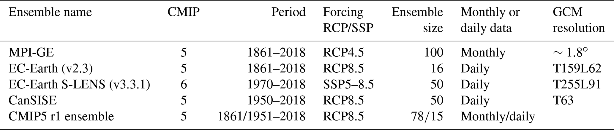
We use five global climate model (GCM) ensembles as listed in Table 2: (i) one member (r1) from each GCM in the CMIP5 (Phase 5 of the Coupled Model Intercomparison Project) multi-member ensemble (Taylor et al., 2012), (ii) the 100-member MPI–ESM grand ensemble (Maher et al., 2019), (iii) the 50-member CanSISE grand ensemble (Kushner et al., 2018; Scinocca et al., 2016), (iv) the 16-member EC-Earth (CMIP5 version) ensemble from Royal Netherlands Meteorological Institute (KNMI; Aalbers et al., 2018), and (v) the 50-member EC-Earth (S-LENS, Doescher et al., 2020; CMIP6 version, Eyring et al., 2016) ensemble from SMHI. The climate models have been run with forcing conditions representing those observed in 1860–2005 following either the CMIP5 or the CMIP6 protocols. From 2006 onward, climate models (i–iv) have been forced by the RCP (Representative Concentration Pathway) scenarios representing future conditions (RCP, Moss et al., 2010). For the S-LENS ensemble, EC-Earth has been forced by the SSP5–8.5 (Shared Socioeconomic Pathway) scenario from 2016 and by observed forcing until 2015 (Riahi et al., 2017). Although SSP5–8.5 is not identical to RCP8.5 forcing, it is the trajectory that is closest to the RCP8.5 pathway (Meinshausen et al., 2020). Most models have been forced by the RCP8.5 (or SSP5–8.5) scenario, whereas MPI-GE has been forced by RCP4.5. For all models, except EC-Earth S-LENS, the scenario forcing starts with the year 2006. As differences in radiative forcing between these scenarios are small in the first decades of the 21st century, we neglect any differences between the scenarios. Details related to time periods, the temporal resolution of temperature data, the forcing conditions, and the size of the respective model ensembles are given in Table 2. In total, we analyse 294 simulations, expanding the sample size for each 30-year period to 8820 (30 summers × 294 simulations). The larger sample increases the possibility of assessing statistically robust probabilities of heat events.
2.3 Variables and indices
All analyses are based on either daily or monthly temperature data. We look at both the daily average and daily maximum temperatures as well as the monthly means of daily average temperature. To assess the average temperature for the summer season, we use monthly mean temperatures for four individual summer months (May–August) separately as well as for two respective summer seasons (JJA, MJJA; seasonal average). Temperature anomalies are calculated against the 1981–2010 reference period.
Furthermore, three warm day indices, based on daily values, are used to assess the temperature variability during summer: (i) the total number of warm days per year (totWarmD); (ii) the maximum number of consecutive warm days per year (max_conWarmD); and (iii) the number of heat events (tot_event), where an event is defined as a minimum of 3 consecutive days of Tmax>threshold.
For simplicity, we define a warm day as a day i with Tmax,i greater than a relative threshold. The threshold is the 95th percentile calculated from all Tmax in May to August (MJJA) during the reference period (see Eq. 1).
This simple definition based on a relative measure is chosen to make it possible to compare conditions in different parts of Sweden to one another. For example, a perceived heatwave in the colder north of Sweden may not even appear in an analysis involving an absolute threshold representative of conditions in southern parts of the country, such as summer days defined as days with Tmax>25 ∘C. Other examples of benefits of a relative measure involve the comparison of coastal and inland stations or between low- and high-altitude stations, for similar reasons.
Additionally we calculate two commonly used heatwave indices. The first of these indices is the warm spell duration index (WSDI, Orlowsky and Seneviratne, 2012) which can be compared to max_conWarmD, although they differ in their definition of a warm day. The WSDI is calculated based on an individual threshold for each day of the year. A warm day is defined as a day with Tmax,i larger than the 90th percentile of Ai, as defined in Eq. (2) (from Eq. (1) in Russo et al., 2014):
where ∪ denotes the union of sets, and is the daily maximum temperature of day d in year y.
The WSDI is determined as the maximum number of consecutive warm days (larger than 3), e.g. for a given year (or season); thus, the WSDI is the longest duration of any such heatwave event.
The second heatwave index is the heat wave magnitude index (HWMI, Russo et al., 2014), which uses the same warm day definition as WSDI. Whereas the WSDI only takes the duration into account, the HWMI also considers the magnitude of the heatwave. The HWMI accounts for multiple local maxima of an event by summing them up and mapping them to a probability (called magnitude) related to annual maximum magnitudes of the reference period. Thus, it weights the duration more than the absolute maximum temperature of an event. This relates to the heat stress that builds up due to many warm days in a row rather than a couple of very warm days in a row (e.g. Notely et al., 2018). A more detailed description of how to calculate the HWMI can be found in Russo et al. (2014).
The analysis is carried out for all model ensembles where respective data are available. Thus, the pdf analysis based on monthly data includes all five ensembles (cf. Table 2 and Table S1 in the Supplement), whereas the warm day indices are based on daily temperature values which are not available from MPI-GE.
The analysis is performed in four steps. First, the observed temperature climate of summer 2018 in Sweden is set into a long-term 250-year perspective by comparing it to the Stockholm series; it is then set into a wider Swedish context by comparing it to observational data from SMHI and to E-OBS. Next, we investigate the extent to which the five GCMs represent warm summer conditions over the reference period (1981–2010) by comparing the GCM ensembles to the observed climate. We also investigate the extent to which conditions in Sweden in the summer of 2018 fall within the simulated ensembles and, therefore, infer the extent to which it could be considered extreme. Finally, we look at the GCM ensembles to address the question of whether a warm summer, such as that observed in 2018, would have been probable in a historical context by comparing it to pre-industrial (1861–1890) and mid-20th-century (1951–1980) conditions. The analysis is first presented for monthly and seasonal mean data in Sect. 3.1 and then repeated in Sect. 3.2 for the indices based on daily temperature data.
3.1 How extreme was the summer of 2018 in Sweden on a monthly and seasonal basis?
For Stockholm, the mean MJJA temperature in 2018 was 17.8 ∘C, which is 3.0 K above the mean for 1998–2017 or 4.0 K above the 1756–1900 mean. The temperature anomalies in Stockholm for each day in 2018 with respect to the long-term 250-year climatological average of 1756–2005 are displayed in Fig. 1. The figure clearly shows that the extended summer, ranging from May to mid-August, yielded a large number of days with temperatures that far exceeded the long-term mean. As shown by Sinclair et al. (2019), the large-scale circulation was dominated by persistent blocking high-pressure systems over Scandinavia in May as well as large parts of July and early August. In June, the situation was different with more low-pressure-dominated weather in northern Scandinavia, whereas the southernmost regions were under the influence of a high-pressure ridge over western Europe. This resulted in lower temperatures, which mainly occurred in northern Sweden but also episodically in southern Sweden, associated with intrusions of cooler air from the west and north-west. The episodes of relatively colder conditions in June can be seen in the Stockholm record, as illustrated in Fig. 1 by blue downward facing spikes.
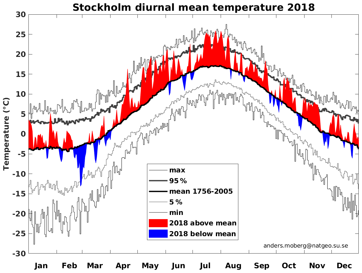
Figure 1Diurnal mean temperatures in Stockholm in 2018. For each day, the anomaly with respect to the 250-year climatological mean for 1756–2005 is displayed in red (warm) or blue (cold). The diagram also shows the warmest and coldest diurnal mean temperature for each calendar day recorded within the 1756–2005 period as well as the corresponding 5th and 95th percentiles.
For the full 4-month period of MJJA, we note that more than 35 % of the days were above the long-term (1756–2005) climatological 95th percentile calculated for each day (thick grey line in Fig. 1). This was indeed a unique feature for 2018. Only 1 additional year, the year 2002, exceeds the 95th percentile of the long-term climatology with 20 % of the days considering a May–August season. Additionally, only 10 other years have 15 % of days exceeding the 95th percentile for MJJA, indicating that a summer, such as 2018, with a very large number of warm days, is rare in a long-term historical perspective. This result is confirmed by the study of Hoy et al. (2020), who analysed 67 long time series all over Europe and found that 33 stations showed the summer half-year of 2018 to be the warmest on record. Hoy et al. (2020) also showed that the Stockholm time series peaks in 2018 for 9 out of 10 of their analysed heatwave indicators (Figs. 5 and 10 in Hoy et al., 2020). An example of this is the hot days (HD) with a maximum temperature above 30 ∘C indicator, which was observed to be 8 d over the previous record (18 d); the heatwave duration indicator, which was 22 d compared with the previous record of 11 d; and the heatwave intensity (HW95, sum of daily excess maximum temperatures > P95), which was 65 K compared with 35 K in 1975 (Hoy et al., 2020, Fig. 7). Another peculiar observation in Fig. 1 is that most individual daily mean temperatures in summer 2018 were not exceptionally warm when viewed individually. In the May–August season, it was rather the large total number of days with temperatures above the long-term climatological 95th percentile that was unique, of which most occurred in May and the second half of July.
Zooming out to the larger scale by exploring the observed monthly data over Sweden, we note that the long-term MJJA 2018 average was 2.8 K above the 1981–2010 mean. This is more than 0.7 K above the second warmest MJJA period recorded in 2002. Compared with the historical data from 1860, there is a clear indication of higher average seasonal mean temperatures over the last few decades. The mid-20th-century period (1951–1980) is 0.6 K warmer on average than the pre-industrial (1861–1890) mean. The difference compared with 1861–1890 increases to 1.2 K for 1981–2010 and to 1.5 K for 1989–2018. Furthermore, 12 out of the 16 (corresponding to the 10th percentile) warmest MJJA periods in the last 160 years (1860–2019) occur after 1988.
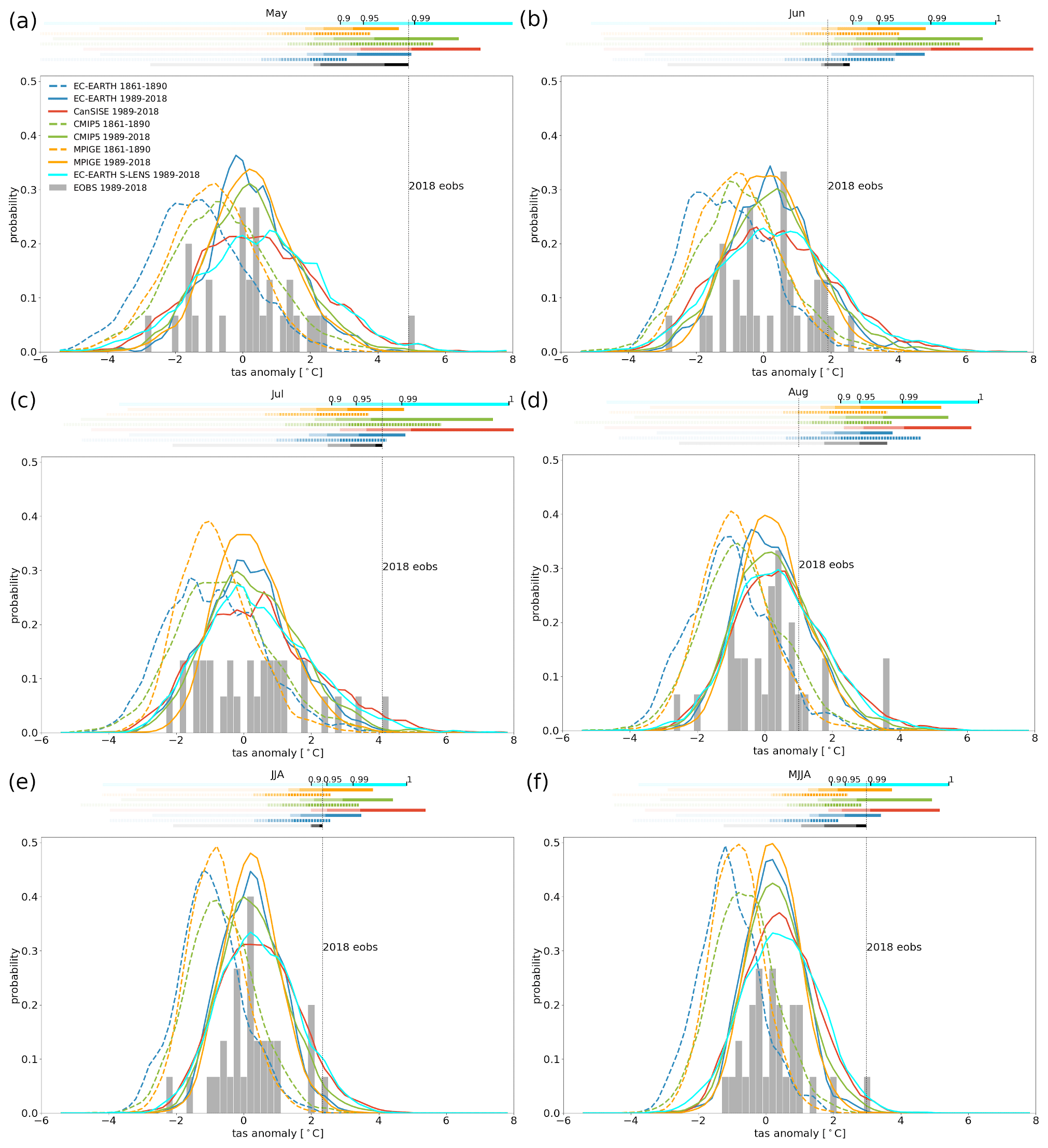
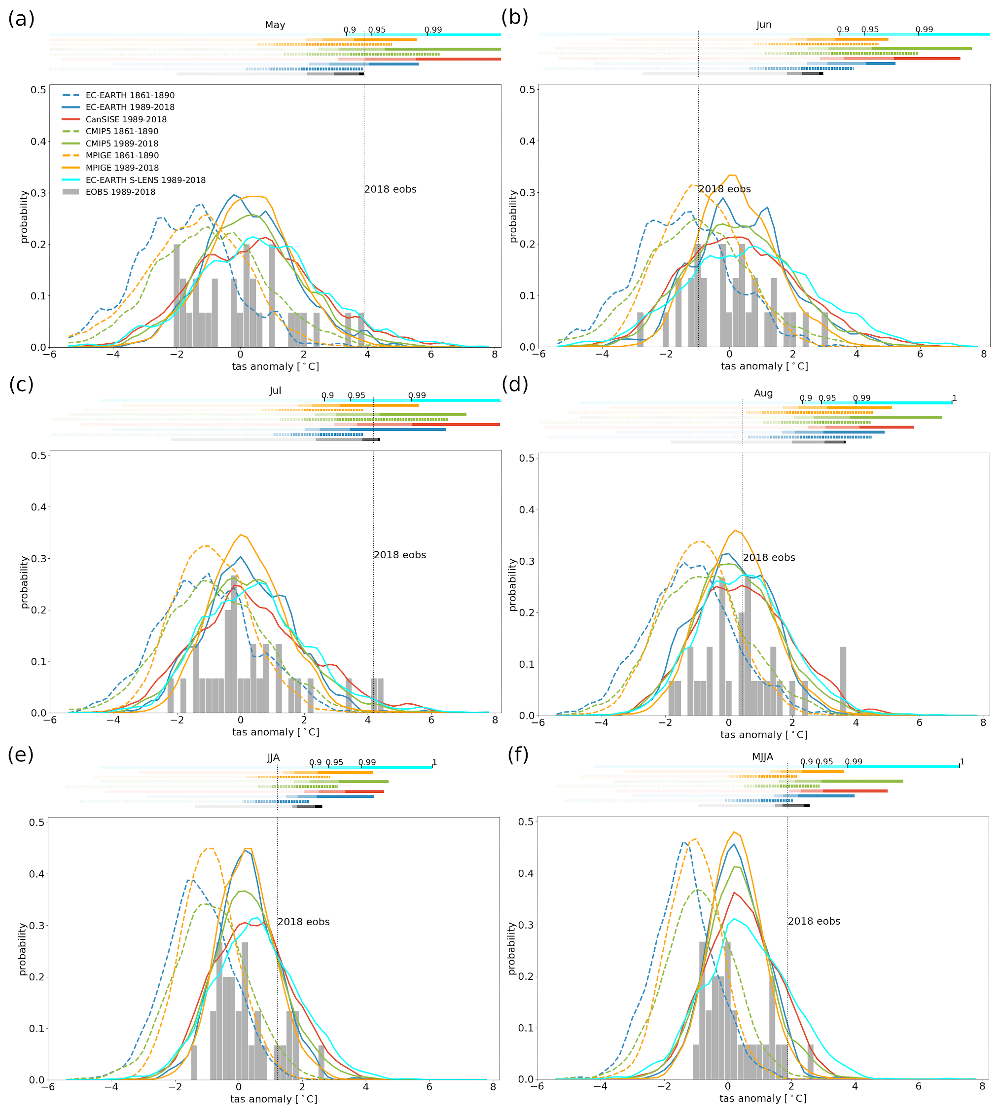
Figure 2Probability distributions for monthly average temperature anomalies, calculated for 1861–1890 (dashed) and 1989–2018 (solid) against 1981–2010 for the southern half of Sweden, for the individual months of May–August as well as seasonally pooled for JJA and MJJA respectively. The bars in the upper part of each panel are a guide to compare the positions of percentiles for each ensemble and period. The opacity of the bars indicates (in steps) the 90th, 95th, 99th, and 100 percentile ranges marked on the uppermost bar. Ensemble distributions are a kernel density fit, whereas the histogram for E-OBS is based on actual data. The observed year 2018 for respective months or season is indicated by the vertical dotted black line.
Probability distributions (pdfs) of the four individual summer months (May–August) from E-OBS temperature data in Fig. 2a–d further illustrate the rarity of the weather situation in 2018 in southern Sweden. This can be seen as May (Fig. 2a) and July (Fig. 2c) 2018, indicated by the dotted line, set the 100 % mark on the extreme warm tail of the observation distribution for the last few decades (grey histogram). June (Fig. 2b) and August (Fig. 2d) were also warmer than normal in southern Sweden, although not within the extreme tail, with June just above the 95th percentile and August well below the 90th percentile. For northern Sweden the picture is similar for May, July, and August, although June 2018 was in fact colder than average in this region, by about 1 K (see Fig. 3), due to low-pressure intrusions. We note that the monthly mean temperatures of May 2018 are the highest observed for May in all 25 Swedish provinces to date according to SMHI observations (not shown).
Pooling the single months together to form JJA and MJJA distributions (Fig. 2e, f), it can be seen that 2018 is the most extreme summer in southern Sweden in the past 30 years according to the E-OBS data set. Moreover, in northern Sweden, the summer of 2018 was more than 1 K warmer than average, but it was far from being among the warmest years (Fig. 3e, f). The extended summer period (MJJA) in 2018 is just above the 95th percentile in northern Sweden and is the second warmest event in the 1989–2018 period.
The climate simulations shown in Figs. 2 and 3 reveal a smoother picture compared with the observations, as we have pooled all of the members of one ensemble together into one probability distribution (solid coloured lines).
For the recent past period (1989–2018), five GCM ensembles (see Table 2) were available, and despite their varying ensemble size and different models, the probability distributions peak at similar monthly and seasonal mean temperature anomalies. We note, however, that even if the average anomalies are similar, there are differences in the spread of the individual ensemble members, as reflected by the different width and height of the probability distributions.
The 1989–2018 ensemble medians show temperature increases exceeding those of the reference period (1981–2010) by between 0.19 K in E-OBS and 0.44 K in EC-Earth-LENS for MJJA conditions.
Compared with the spread in observed temperatures as derived from E-OBS, all five GCM ensembles include summers as warm (or as cold) as any individual observed summer during the 1989–2018 period, both for individual months and for the 3- and 4-month-long summer seasons. May 2018 is, however, an exception to this, as it is warmer than all of the 100 simulated May months in the MPI-GE for southern Sweden. The fact that the GCM ensembles generally show a larger spread than that of the observations is not surprising, as they constitute a large number of realizations and, in turn, many 30-year periods representing the recent past climate, whereas the E-OBS data only represent one such period. The assessment presented here is not a full evaluation of the ability of the models to represent summertime temperatures in Sweden. However, the coverage of the E-OBS probability distribution within the GCM ensembles lends confidence in the climate models.
For northern Sweden, the models show a similar agreement as in southern Sweden regarding the position of the peak for each month or season (Fig. 3). Even though the observed May and July temperatures are the highest in the last 30 years, the model ensembles indicate that temperatures as high as those observed in 2018 are more likely to occur again in the north than in the south. The probabilities are, however, still low, being below 5 % for most of the model ensembles. Compared with southern Sweden, June and August 2018 were relatively mild in northern Sweden. For June, 2018 was even on the cooler side of the monthly temperature distributions.
Even if only May 2018 is completely outside of one of the GCM ensembles in southern Sweden, it is clear that both May and July as well as the JJA and MJJA summer seasons in 2018 stand out as being warm or very warm in the context of the large model ensembles.
Three ensembles include pre-industrial data, giving us the opportunity to compare the recent past climate and the year 2018 with the pre-industrial period (1861–1890). We also carry out a comparison with the mid-20th-century period (1951–1980) in order to be consistent with the analysis of daily data in Sect. 3.2. Here, the observed May 2018 temperatures in southern Sweden are outside of all climate model ensembles for 1861–1890 apart from the CMIP5 multi-model ensemble (dashed lines and bars in Fig. 2). However, the probability of such a warm month is also below 1 % in CMIP5 (Fig. 2a). The other two GCMs, MPI-GE and EC-Earth, do not include such a warm May in any of their ensemble members, not even for the mid-20th-century period (1951–1980; not shown). Again, when pooling the months to MJJA, none of the ensembles actually simulate temperature anomalies as high as those in 2018 for southern Sweden in the pre-industrial period (Fig. 2f dashed lines) nor in the mid-20th century. This also indicates that CMIP5 temperatures like those in May 2018 only fall into the distribution because of the chosen fit of the Gaussian pdf estimate. (The pdf curve continues smoothly to zero even if there is no value at the end of the tail.) Even if conditions in northern Sweden were not as extreme, with the relatively cooler June and August months, it is clear that the probability of a summer (MJJA) as warm as that observed in 2018 is less than 1 % in all ensembles (Fig. 3).
3.2 How extreme was the warm summer of 2018 in Sweden on an event basis?
As a heatwave is not only perceived by monthly averages, we calculated five different indices to account for different characteristics of extreme and long-lasting events (see Sect. 2.3): the total number of warm days (totWarmD), the maximum number of consecutive warm days representing the longest heat event (max_conWarmD), the number of heat events lasting at least 3 days (tot_event), the heat wave magnitude index (HWMI), and the warm spell duration index (WSDI). These indices are calculated for the extended summer period (MJJA). As they are all based on maximum daily temperature data, which are only available from 1951 for most of the simulations (see Table 2), we compare the mid-20th century (1951–1980) to the present-day period (1989–2018).
Figure 4a reveals that a total of 28 warm days (totWarmD) are found for southern Sweden in MJJA 2018 according to E-OBS. It is clear that this puts MJJA 2018 on the extreme end of the distribution and well above any other years. Comparing the observations for 1989–2018 with those for 1951–1980 shows that the distribution of totWarmD has widened and the mean and median (red mark) have concurrently been shifted towards more warm days. Moreover, the model ensembles agree on that message, with CanSISE showing the strongest change signal between the two periods. Looking at the most extreme summers, it is clear that all models indicate an increase in the 95th percentile (upper whisker) and show larger absolute maxima. For three out of four model ensembles, more summers with more than 28 warm days can be found in the present-day period compared with the mid-20th-century period. We also note that both observations and models indicate that there is a tendency for summers without any warm days to become less frequent with time. From Fig. 4b, we see that 28 warm days would only have been reached once in the simulated pre-industrial climate (in the 1860s), although this was only represented by one ensemble.
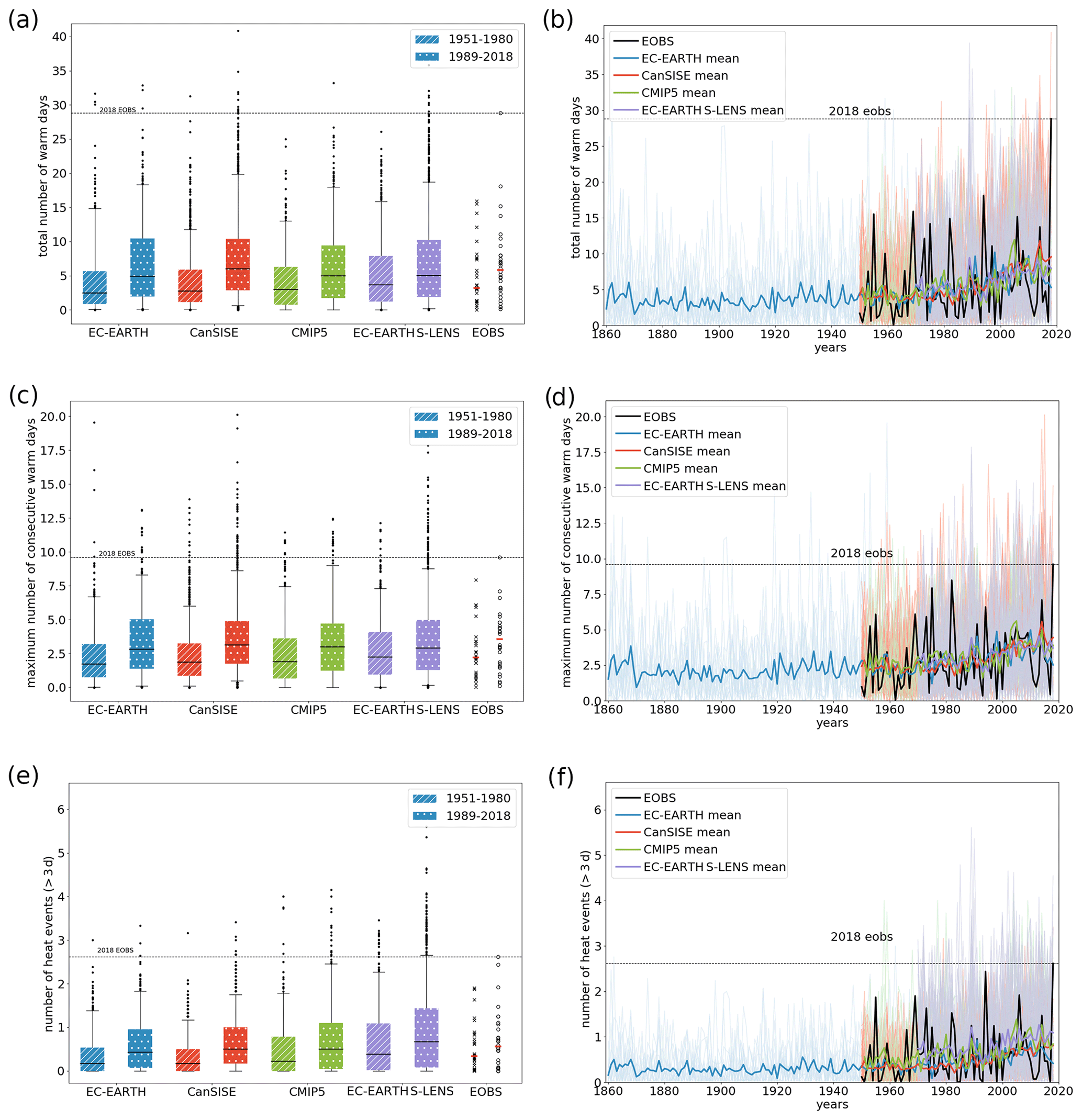
Figure 4The left column shows (a) the total number of warm days (totWarmD), (c) the maximum number of consecutive warm days (max_conWarmD), and the (e) number of heat events (tot_events) for the 1951–1980 (dashed) and 1989–2018 (dotted) periods for four models (x axis), calculated from the MJJA months and averaged over southern Sweden. All model members are pooled into one box. Corresponding data for E-OBS are shown to the right with the red mark indicating the median. The right column shows time series for each ensemble member (thin lines) and ensemble means (bold lines) for (b) totWarmD, (d) max_conWarmD, and (f) tot_event. The number of days for 2018 as derived from E-OBS is indicated by the horizontal dashed line.
The maximum number of consecutive warm days (max_conWarmD) reflects another aspect of warm days. This is important, as extended periods with warm conditions have a stronger impact on human health as well as on other parts of nature than a single heat day (e.g. Oudin Åström et al., 2013; Rasmont and Iserbyt, 2012). Figure 4d shows the time series for max_conWarmD where the thin coloured lines represent the single ensemble members, the bold lines represent the ensemble means, and the horizontal dotted black line indicates the max_conWarmD value of 2018 as calculated from E-OBS. The figure also shows that observed variability from E-OBS (black solid line) lies within the variability of all simulations and that 2018 does not stand out as being among the most extreme summers in the period. The sharp peaks for the single ensemble members indicate high year-to-year variability of max_conWarmD for each member as well as for the other indices (Fig. 4b, d, f).
The warming signal starting in the few last decades of the 20th century is clearly visible for all four ensembles, although it is particularly visible when referring to the long time series of EC-Earth. The time series also show that the summer 2018 max_conWarmD value is exceeded much more often in recent years than in earlier times, shifting the summer 2018 event towards the centre of the distributions. Figure 4c shows the change in all ensembles towards longer events with more consecutive warm days going from 1951–1980 to 1989–2018. However, it is clear that summer 2018 is still outside the whiskers in the figure, indicating that it is above the 95 % range for all ensembles. Again, as for the totWarmD (Fig. 3a), the lower whisker changes towards the present-day climate by starting to lift from zero (lower boundary).
The median max_conWarmD is very similar for all ensembles at about 2 and 3 d for the 1951–1980 and 1989–2018 periods respectively (cf. black median lines in the boxes in Fig. 4c). The maximum value ranges from 12 to 20 d for all ensembles and both periods. These results are very similar to Zschenderlein et al. (2019), who found a maximum heatwave duration of 12 d. We find this close similarity despite differences in the data set, the periods, the exact definition of the index, and the regions not being identical.
Furthermore, the total number of heat events (tot_event) reveals that summer 2018 was an unusual event with more heat events than covered by ensemble simulations for the historical time period (Fig. 4e, f). It is also leading the extreme tail, even for the present-day climate. The ensemble means show a clear upward trend at the end of the 20th century and the pooled distribution indicates a similar detachment from zero as discussed above for max_conWarmD. Moreover, the observations show a detachment from the zero lower limit in the most recent 20 years (Fig. 4f). As for the totWarmD (Fig. 4b), only 1 year in the pre-industrial climate has been simulated above the summer 2018 value by the EC-Earth model (Fig. 4f).
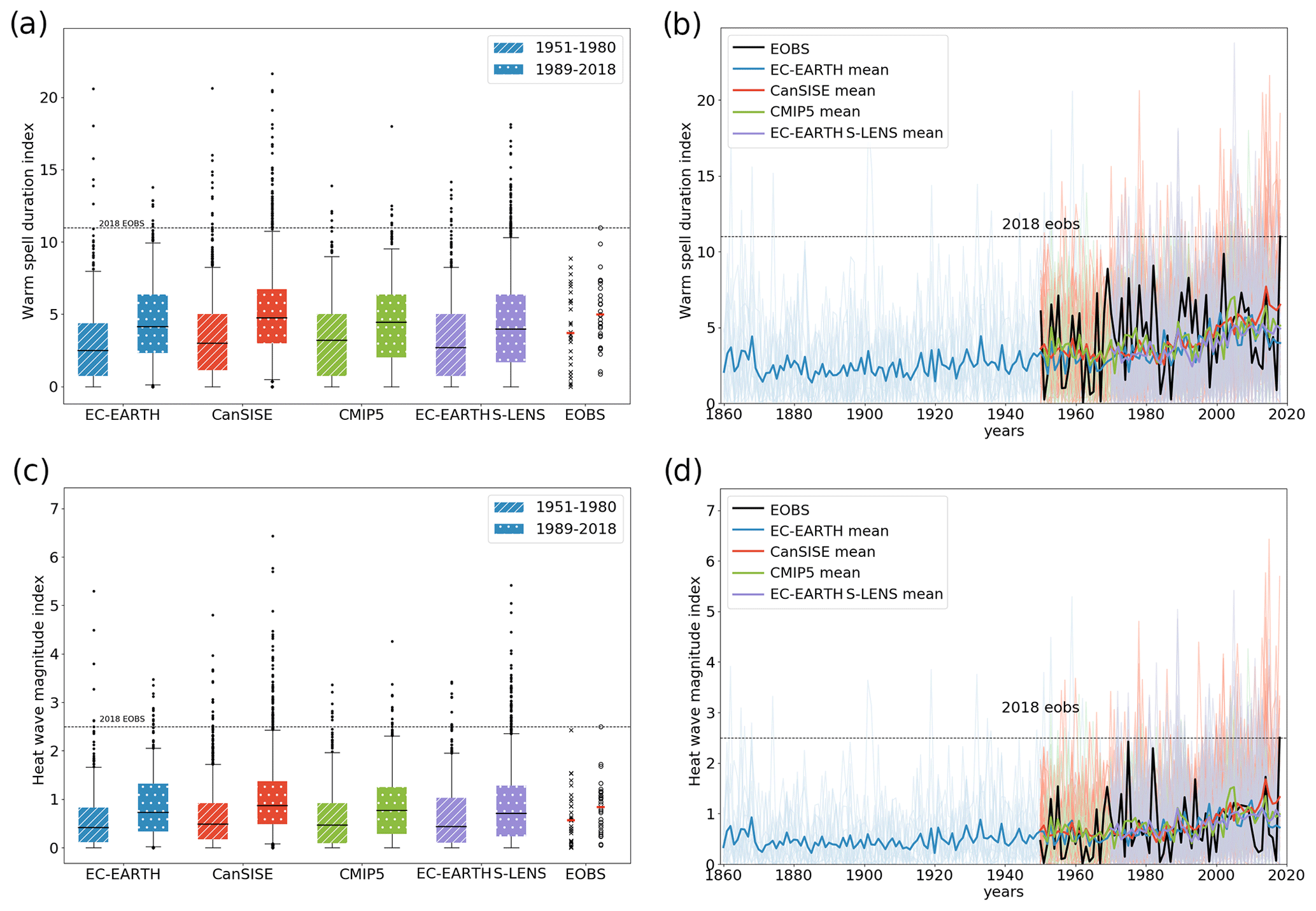
The picture of more extensive and intense heatwaves, as indicated above, is manifested in all indices. The more complex heat indices WSDI and HWMI also support this finding. Figure 5a shows the WSDI for each ensemble pooled using box-whiskers and the WSDI for 2018 based on E-OBS as a dotted horizontal line. For WSDI, the summer 2018 is on the extreme tail for all ensembles and periods. It again shows a clear upward shift of all distributions towards the summer 2018 value. The time series analysis of E-OBS indicates that 2018 stands out relative to any other year observed since 1951. At the same time, however, WSDI numbers as high as that observed in 2018 do occur in the model ensembles for 1989–2018, reaching almost the 5 % level in the CanSISE model.
HWMI (Fig. 5c, d) also follows the main picture described above. The summer 2018 value of 2.5 indicates a moderate heatwave magnitude (Russo et al., 2014) that does occur in all ensembles, although only with relatively low probabilities. Figure 5d shows that the observed HWMI varies between 0 and 2.5 for southern Sweden with a mean that increases from about 0.7 in the mid-20th century to 0.9 at the beginning of the current century.
3.3 Discussion
In this study, we assess the degree to which summer 2018 in Sweden can be considered an extreme event. Without doubt, the summer was remarkably warm and in some aspects way beyond what has been observed for Sweden as a whole for the last 160 years and for Stockholm in a 250 year perspective. However, the results also clearly show that the degree of rarity of the summer is very different depending on which measure is investigated. The monthly mean temperature for May and the number of warm days above the 95th percentile in MJJA are examples for which 2018 is the most extreme summer observed to date. For other indices, such as the WSDI, results indicate less extreme conditions compared with other years. Such differences may simply be the result of looking at different aspects of warm summers, but they may also be a result of different methods; for example, in this case, the difference may stem from using a fixed threshold relative to an index based on a day-to-day evolving threshold. As an example of how results may be different depending on the definition, we note that when May is not included as a summer month and we focus on the more commonly used generic 3-month JJA summer, summer 2018 was not as remarkable. In particular, in light of the large ensembles, such a warm JJA summer is found in single members of all of the assessed climate model ensembles even in the pre-industrial climate. Such a definition would make the study more comparable to other summer studies, but the impact of long-lasting heat events would be missed if an early onset of summer temperatures was not included.
An implication of our findings is that attribution statements based on specific features of a part of a season can not be taken as being representative of a more general full-season perspective and vice versa. Yiou et al. (2020) could demonstrate the thermodynamic contribution of human-induced climate change for the Scandinavian heatwave 2018. They found a +5.4 K temperature anomaly for the second and warmer part of the heatwave (19 d at the end of July 2018) over Scandinavia (including Norway, Sweden, Denmark, and Finland) relative to the 1981–2010 reference period. In particular, they found that each single day of this period was at least 3 K above the climatological mean. Yiou et al. (2020) also carried out a probability analysis based on two GCM ensembles and two RCM (regional climate model) ensembles and found that a heat event like the 19 d at the end of July 2018 was 5 to 2000 times more likely in the present-day climate than in the pre-industrial period. This agrees well with our analysis of the five large GCM ensembles.
Leach et al. (2019) stated that the 2018 heatwave over Europe would not have happened without human-induced climate change. For Europe, they found an event like the 2018 summer to be 10 to 100 times more likely in the present-day climate than in the pre-industrial climate.
For all of the aspects of summer temperatures assessed in this study, the five model ensembles present a relatively coherent picture with the central values (medians) and ensemble spreads (e.g. standard deviation or interquartile ranges) being similar. However, for the more extreme values, like the 95th or 99th percentile, differences between ensembles tend to be larger with more systematic differences between them. For instance, the CanSISE and the EC-Earth-LENS ensemble tend to give significantly stronger warm extremes than the ensembles from the previous version of the EC-Earth model and the MPI-GE. We note that for all of the model ensembles assessed here, there are, with few exceptions, always individual summers as extreme as 2018 in the 1989–2018 period. It is difficult to judge, based on the relatively simple evaluation presented here, whether the GCMs are performing well by implying that such summers are, even if rare events, still an existing type of summer in today's climate, or, if the models are overestimating the chance of such a summer. This fundamental uncertainty restricts us from making a formal attribution analysis as we simply do not know which climate to evaluate the models against.
All models suffer from simulation biases. For summer temperatures, all models show a certain cold bias over northern Europe which ranges from −0.2 to −1 K (not shown). However, as the analysis was carried out for each ensemble separately and focused on anomalies, the impact of any systematic bias was reduced.
It is known that GCMs have difficulties capturing many aspects of blocking (e.g. Davini and D'Andrea, 2016; Dawson and Palmer, 2015). Studies on atmospheric blocking representation in the GCMs used here agree on an underestimation of blocking frequency, which mostly occurs in winter but is also seen in summer (EC-Earth: Hartung et al., 2017; CMIP5: Woolings et al., 2018; Masato et al., 2013; Dunn-Sigouin and Son, 2013; MPI-GE: Maher et al., 2019; Müller et al., 2018; CanESM: Schaller et al., 2018; Brunner et al., 2018).
Increasing the horizontal and vertical resolution of GCMs can strongly improve their ability to capture atmospheric blocking (Hartung et al., 2017; Jung et al., 2012). However a positive effect of increased resolution could not be confirmed for summer blocking episodes (Schiemann et al., 2017). Sousa et al. (2018) found that the frequency of summer blocking (23 % of days, and only 9 % of days over Scandinavia) is less than that of winter blocking (35 % of days). The small sample size of summer blocking episodes over northern Europe handicaps statistical analysis; hence, the number of references on that topic is low.
For this study, we focus on the advantage of large ensembles that increase the sample size for the statistical evaluation of high-temperature events.
A more extensive model evaluation exercise that incorporates a rigorous test of the model's ability to simulate extended periods with high-pressure situations such as that observed in 2018, including the temperature conditions during such episodes, is planned for a forthcoming study.
We analyse the temperature conditions in Sweden during summer 2018 in comparison with the observed climate. The results clearly show that summer 2018 stands out as an unusually warm event in relation to the observed climate. We have also shown that the degree of rarity depends on the measure that is evaluated. For instance, we note that the average temperature of the month of May was the most exceptional compared with observations. Moreover, average July temperatures and the 4-month average May–August temperatures are far above previous maxima for southern Sweden, whereas June and August temperatures are more modest. Some other indices, like the warm spell duration index (WSDI) and heatwave magnitude index (HWMI), show less extreme conditions.
We also compare the summer of 2018 with a large number of climate model simulations. Five different global climate model ensembles with a total of 294 climate model simulations have been assessed. This gives us the opportunity to set the observed summer in 2018 in the perspective of 8820 summers over the period from 1989 to 2018. We find that conditions like those observed in summer 2018 do occur in all climate model ensembles. An exception is the monthly mean temperature for May for which 2018 was warmer than any member in one of the climate model ensembles. However, even if the ensembles comprise individual years like 2018, the comparison shows that such conditions are rare. For the indices assessed here, anomalies such as those observed in 2018 occur less than once in 20 years in all ensembles except for the total number of warm events in one of the ensembles. For some indices, the anomalies are even more rare and do not occur more frequently than once in 100 years. We note that there are very large differences between the various models with respect to the degree of probability a summer like 2018 would have. As a consequence, we do not assign specific probabilities but instead discuss the results more qualitatively.
As the simulations also cover historical periods further back in time, we can assess the extent to which conditions have changed over time as a consequence of increased greenhouse warming. For all of the indices evaluated, we find that the probability of a summer like that in 2018 has increased from relatively low values in 1861–1890 and 1951–1980 to higher values in the most recent decades (1989–2018). An implication of this is that anthropogenic climate change has strongly increased the probability of a warm summer, such as the one observed in 2018, occurring in Sweden. Despite this, we still find that such summers also occur in models in the pre-industrial climate, albeit with a lower probability.
The MPI Grand Ensemble is now openly available at https://esgf-data.dkrz.de/projects/mpi-ge/ (last access: 1 December 2020) (Maher et al., 2019); CanSISE data from the CanESM2 model are available online at http://crd-data-donnees-rdc.ec.gc.ca/CCCMA/products/CanSISE/output/CCCma/ (last access: 1 December 2020) (Kushner et al., 2018; Scinocca et al., 2016); the EC-Earth ensemble from KNMI is available at https://climexp.knmi.nl/KNMI14Data/CMIP5/output/KNMI/ECEARTH23/rcp85/ (last access: 1 December 2020) (Aalbers et al., 2018). EC-Earth-LENS is produced by the Swedish Meteorological and Hydrological Institute (SMHI) and can be made available upon request. The ensemble will be uploaded to the Earth System Grid Federation (ESGF) during 2020. CMIP5 data are openly available via ESGF data nodes. The Stockholm daily mean temperature series is available at https://doi.org/10.17043/stockholm-historical-temps-daily-2 (Moberg, 2020).
The supplement related to this article is available online at: https://doi.org/10.5194/esd-11-1107-2020-supplement.
RAIW and EK designed the structure of the experiment and the document and did most of the writing. RAIW carried out the analysis on the temperature and three indices. EK performed the analysis on observations. CL undertook the analysis on HWMI and WSDI. AM carried out the analysis on the Stockholm time series. DM and ET provided the ensemble data from the MPI climate modelling group (as it was not openly available at the beginning of this study). All authors commented on the results and helped revise the paper.
The authors declare that they have no conflict of interest.
The authors are grateful to Lennart Wern at SMHI for providing the monthly mean temperature data. The authors acknowledge the World Climate Research Programme's Working Group on Coupled Modelling, which is responsible for CMIP, and we thank the climate modelling groups (listed in Table S1) for producing their model output and making it available.
This study was supported by FORMAS (REGTREND, EDUCAS) and the EUCP project, which is funded by the European Commission through the Horizon 2020 Research and Innovation programme (grant no. 776613). The research leading to these results has also received funding from the German Federal Ministry of Education and Research (BMBF) through the JPI Climate/Belmont Forum InterDec project (FKZ grant no. 01LP1609A to Evangelos Tyrlis and Daniela Matei) and JPI Climate/JPI Oceans NextG-Climate Science-ROADMAP (FKZ grant no. 01LP2002A to Daniela Matei).
This paper was edited by Sagnik Dey and reviewed by two anonymous referees.
Aalbers, E. E., Lenderink, G., van Meijgaard, E., and van den Hurk, B. J. J. M.: Local-scale changes in mean and heavy precipitation in Western Europe, climate change or internal variability?, Clim. Dynam., 50, 4745, https://doi.org/10.1007/s00382-017-3901-9, 2018.
Alexandersson, H. and Eggertsson Karlström, C.: Temperaturen och nederbörden i Sverige 1961–1990, Referensnormaler – utgåva 2, SMHI, reports Meteorologi, 99, SMHI, Norrköping, Sweden, 71 pp., ISSN 0283-7730, 2001.
Alexandersson, H. and Moberg, A.: Homogenization of Swedish Temperature data. PART I: Homogeneity Test for Linear Trends, Int. J. Climatol., 17, 25–34, https://doi.org/10.1002/(SICI)1097-0088(199701)17:1<25::AID-JOC103>3.0.CO;2-J, 1997.
Åström, C., Bjelkmar, P., and Forsberg, B.: Attributing summer mortality to heat during 2018 heatwave in Sweden, Environ. Epidemiol., 3, 16–17, https://doi.org/10.1097/01.EE9.0000605788.56297.b5, 2019.
Brunner, L., Schaller, N., Anstey, J., Sillmann, J., and Steiner, A. K.: Dependence of present and future European temperature extremes on the location of atmospheric blocking, Geophys. Res. Lett., 45, 6311–6320, https://doi.org/10.1029/2018GL077837, 2018.
Buras, A., Rammig, A., and Zang, C. S.: Quantifying impacts of the 2018 drought on European ecosystems in comparison to 2003, Biogeosciences, 17, 1655–1672, https://doi.org/10.5194/bg-17-1655-2020, 2020.
Davini, P. and D'Andrea, F.: Northern Hemisphere Atmospheric Blocking Representation in Global Climate Models: Twenty Years of Improvements?, J. Climate, 29, 8823–8840, https://doi.org/10.1175/JCLI-D-16-0242.1, 2016.
Dawson, A. and Palmer, T. N.: Simulating weather regimes: Impact of model resolution and stochastic parameterization, Clim. Dynam., 44, 2177–2193, https://doi.org/10.1007/s00382-014-2238-x, 2015.
Deser, C., Phillips, A., Bourdette, V., and Teng, H.: Uncertainty in climate change projections: the role of internal variability, Clim. Dynam., 38, 527–546, https://doi.org/10.1007/s00382-010-0977-x, 2012.
Doescher, R. and the EC-Earth Consortium: The EC-Earth3 Earth System Model for the Climate Model Intercomparison Project 6, in preparation, 2020.
Dunn-Sigouin, E. and Son, S.-W.: Northern Hemisphere blocking frequency and duration in the CMIP5 models, J. Geophys. Res.-Atmos., 118, 1179–1188, https://doi.org/10.1002/jgrd.50143, 2013.
Eyring, V., Bony, S., Meehl, G. A., Senior, C. A., Stevens, B., Stouffer, R. J., and Taylor, K. E.: Overview of the Coupled Model Intercomparison Project Phase 6 (CMIP6) experimental design and organization, Geosci. Model Dev., 9, 1937–1958, https://doi.org/10.5194/gmd-9-1937-2016, 2016.
Hartung, K., Svensson, G., and Kjellström, E.: Resolution, physics and atmosphere–ocean interaction – How do they influence climate model representation of Euro-Atlantic atmospheric blocking?, Tellus A, 69, https://doi.org/10.1080/16000870.2017.1406252, 2017.
Haylock, M. R., Hofstra, N., Klein Tank, A. M. G., Klok, E. J., Jones, P. D., and New, M.: A European daily high-resolution gridded data set of surface temperature and precipitation for 1950–2006, J. Geophys. Res., 113, D20119, https://doi.org/10.1029/2008JD010201, 2008.
Hoy, A., Hänsel, S., and Maugeri, M.: An endless summer: 2018 heat episodes in Europe in the context of secular temperature variability and change, Int. J. Climatol., https://doi.org/10.1002/joc.6582, in press, 2020.
Humborg, C., Geibel, M.C., Sun, X., McCrackin, M., Mörth, C.-M., Stranne, C., Jakobsson, M., Gustafsson, B., Sokolov, A., Norkko, A., and Norkko, J.: High Emissions of Carbon Dioxide and Methane From the Coastal Baltic Sea at the End of a Summer Heat Wave, Front. Mar. Sci., 6, 493, https://doi.org/10.3389/fmars.2019.00493, 2019.
IPCC: Managing the Risks of Extreme Events and Disasters to Advance Climate Change Adaptation, in: A Special Report of Working Groups I and II of the Intergovernmental Panel on Climate Change, edited by: Field, C. B., Barros, V., Stocker, T. F., Qin, D., Dokken, D. J., Ebi, K. L., Mastrandrea, M. D., Mach, K. J., Plattner, G.-K., Allen, S. K., Tignor, M., and Midgley, P. M., Cambridge University Press, Cambridge, UK and New York, NY, USA, 582 pp., 2012.
IPCC: Global warming of 1.5 ∘C, in: An IPCC Special Report on the impacts of global warming of 1.5 ∘C above pre-industrial levels and related global greenhouse gas emission pathways, in the context of strengthening the global response to the threat of climate change, sustainable development, and efforts to eradicate poverty, edited by: Masson-Delmotte, V., Zhai, P., Pörtner, H. O., Roberts, D., Skea, J., Shukla, P. R., Pirani, A., Moufouma-Okia, W., Péan, C., Pidcock, R., Connors, S., Matthews, J. B. R., Chen, Y., Zhou, X., Gomis, M. I., Lonnoy, E., Maycock, T., Tignor, M., and Waterfield, T., in press, 2018.
Jung, T., Miller, M. J., Palmer, T. N., Towers, P., Wedi, N., Achuthavarier, D., Adams, J. M., Altshuler, E. L., Cash, B. A., Kinter, J. L., Marx III, L., Stan, C., and Hodges, K. I.: High-resolution global climate simulations with the ECMWF model in Project Athena: Experimental design, model climate, and seasonal forecast skill, J. Climate, 25, 3155–3172, https://doi.org/10.1175/JCLI-D-11-00265.1, 2012.
Kirchmeier-Young, M. C., Wang, H., Zhang, X., and Seneviratne, S. I.: Importance of framing for extreme event attribution: The role of spatial and temporal scales, Earth's Future, 7, 1192–1204, https://doi.org/10.1029/2019EF001253, 2019.
Krikken, F., Lehner, F., Haustein, K., Drobyshev, I., and van Oldenborgh, G. J.: Attribution of the role of climate change in the forest fires in Sweden 2018, Nat. Hazards Earth Syst. Sci. Discuss., https://doi.org/10.5194/nhess-2019-206, in review, 2019.
Kushner, P. J., Mudryk, L. R., Merryfield, W., Ambadan, J. T., Berg, A., Bichet, A., Brown, R., Derksen, C., Déry, S. J., Dirkson, A., Flato, G., Fletcher, C. G., Fyfe, J. C., Gillett, N., Haas, C., Howell, S., Laliberté, F., McCusker, K., Sigmond, M., Sospedra-Alfonso, R., Tandon, N. F., Thackeray, C., Tremblay, B., and Zwiers, F. W.: Canadian snow and sea ice: assessment of snow, sea ice, and related climate processes in Canada's Earth system model and climate-prediction system, The Cryosphere, 12, 1137–1156, https://doi.org/10.5194/tc-12-1137-2018, 2018.
Leach, N., Li, S., Sparrow, S., van Oldenborgh, G. J., Lott, F. C., Weisheimer, A., and Allen, M. J.: Anthropogenic influence on the 2018 summer warm spell in Europe: the impact of different spatio-temporal scales, B. Am. Meteorol. Soc., 101, S41–S46, 2019.
Maher, N., Milinski, S., Suarez-Gutierrez, L., Botzet, M., Dobrynin, M., Kornblueh, L., Kröger, J., Takano, Y., Ghosh, R., Hedemann, C., Li, C., Li, H., Manzini, E., Notz, N., Putrasahan, D., Boysen, L., Claussen, M., Ilyina, T., Olonscheck, D., Raddatz, T., Stevens, B., and Marotzke, J.: The Max Planck Institute Grand Ensemble: Enabling the Exploration of Climate System Variability, J. Adv. Model. Earth Syst., 11, 1–21, https://doi.org/10.1029/2019MS001639, 2019.
Masato, G., Hoskins, B. J., and Woollings, T.: Winter and Summer Northern Hemisphere Blocking in CMIP5 Models, J. Climate, 26, 7044–7059, https://doi.org/10.1175/JCLI-D-12-00466.1, 2013.
Meinshausen, M., Nicholls, Z., Lewis, J., Gidden, M. J., Vogel, E., Freund, M., Beyerle, U., Gessner, C., Nauels, A., Bauer, N., Canadell, J. G., Daniel, J. S., John, A., Krummel, P., Luderer, G., Meinshausen, N., Montzka, S. A., Rayner, P., Reimann, S., Smith, S. J., van den Berg, M., Velders, G. J. M., Vollmer, M., and Wang, H. J.: The shared socio-economic pathway (SSP) greenhouse gas concentrations and their extensions to 2500, Geosci. Model Dev., 13, 3571–3605, https://doi.org/10.5194/gmd-13-3571-2020, 2020.
Moberg, A.: Stockholm Historical Weather Observations – Daily mean air temperatures since 1756, Dataset version 2.0, Bolin Centre Database, https://doi.org/10.17043/stockholm-historical-temps-daily-2, 2020.
Moberg, A. and Alexandersson, H.: Homogenization of Swedish Temperature data. PART II: Homogenized Gridded Air Temperature Compared with a Subset of Global Gridded Air Temperature since 1861, Int. J. Climatol., 17, 35–54, https://doi.org/10.1002/(SICI)1097-0088(199701)17:1<35::AID-JOC104>3.0.CO;2-F, 1997.
Moberg, A., Bergström, H., Ruiz Krigsman, J., and Svanered, O.: Daily air temperature and pressure series for Stockholm (1756–1998), Climatic Change, 53, 171–212, https://doi.org/10.1023/A:1014966724670, 2002.
Moberg, A., Alexandersson, H., Bergström, H., and Jones, P. D.: Were Southern Swedish summer temperatures before 1860 as warm as measured?, Int. J. Climatol., 23, 1495–1521, https://doi.org/10.1002/joc.945, 2003.
Moberg, A., Tuomenvirta, H., and Nordli, Ø.: Recent climatic trends, in: Physical Geography of Fennoscandia, Oxford Regional Environments Series, edited by: Seppälä, M., Oxford University Press, Oxford, 113–133, 2005.
Moss, R. H., Edmonds, J. A., Hibbard, K. A., Manning, M. R., Rose, S. K., van Vuuren, D. P., Carter, T. R., Emori, S., Kainuma, M., Kram, T., Meehl, G. A., Mitchell, J. F. B., Nakicenovic, N., Riahi, K., Smith, S. J., Stouffer, R. J., Thomson, A. M., Weyant, J. P., and Wilbanks, T. J.: The next generation of scenarios for climate change research and assessment, Nature, 463, 747–756, https://doi.org/10.1038/nature08823, 2010.
Müller, W. A., Jungclaus, J. H., Mauritsen, T., Baehr, J., Bittner, M., Budich, R., Bunzel, F., Esch, M., Ghosh, R., Haak, H., Ilyina, T., Kleine, T., Kornblueh, L., Li, H., Modali, K., Notz, D., Pohlmann, H., Roeckner, E. Stemmler, I., Tian, F., and Marotzke, J.: A higher-resolution version of the Max Planck Institute Earth System Model (MPI-ESM1.2-HR), J. Adv. Model. Earth Syst., 10, 1383–1413, https://doi.org/10.1029/2017MS001217, 2018.
Notley, S. R., Meade, R. D., D'Souza, A. W., McGarr, G. W., and Kenny, G. P.: Cumulative effects of successive workdays in the heat on thermoregulatory function in the aging worker, Temperature, 5, 293–295, https://doi.org/10.1080/23328940.2018.1512830, 2018.
Orlowsky, B. and Seneviratne, S.: Global changes in extreme events: Regional and seasonal dimension, Climatic Change, 110, 669–696, https://doi.org/10.1007/s10584-011-0122-9, 2012.
Oudin Åström, D., Forsberg, B., Ebi, K., and Rocklöv, J.: Attributing mortality from extreme temperatures to climate change in Stockholm, Sweden, Nat. Clim. Change, 3, 1050–1054, https://doi.org/10.1038/nclimate2022, 2013.
Perkins-Kirkpatrick, S. E. and Lewis, S. C.: Increasing trends in regional heatwaves, Nat. Commun., 11, 3357, https://doi.org/10.1038/s41467-020-16970-7, 2020.
Pfahl, S. and Wernli, H.: Quantifying the relevance of atmospheric blocking for co-located temperature extremes in the Northern Hemisphere on (sub-)daily time scales, Geophys. Res. Lett., 39, L12807, https://doi.org/10.1029/2012GL052261, 2012.
Räisänen, J.: Energetics of interannual temperature variability, Clim. Dynam., 52, 3139–3156, https://doi.org/10.1007/s00382-018-4306-0, 2018.
Rasmont, P. and Iserbyt, S.: The Bumblebees Scarcity Syndrome: Are heat waves leading to local extinctions of bumblebees (Hymenoptera: Apidae: Bombus)?, Ann. Soc. Entomol. Fr., 48,, 275–280, https://doi.org/10.1080/00379271.2012.10697776, 2012.
Riahi, K., van Vuuren, D. P., Kriegler, E., Edmonds, J., O'Neill, B. C., Fujimori, S., Bauer, N., Calvin, K., Dellink, R., Fricko, O., Lutz, W., Popp, A., Cuaresma, J. C., KC, S., Leimbach, M., Jiang, L., Kram, T., Rao, S., Emmerling, J., Ebi, K., Hasegawa, T., Havlik, P., Humpenöder, F., Da Silva, L. A., Smith, S., Stehfest, E., Bosetti, V., Eom, J., Gernaat, D., Masui, T., Rogelj, J., Strefler, J., Drouet, L., Krey, V., Luderer, G., Harmsen, M., Takahashi, K., Baumstark, L., Doelman, J. C., Kainuma, M., Klimont, Z., Marangoni, G., Lotze-Campen, H., Obersteiner, M., Tabeau, A., Tavoni, M.: The Shared Socioeconomic Pathways and their energy, land use, and greenhouse gas emissions implications: An overview, Global Environ. Change, 42, 153–168, https://doi.org/10.1016/j.gloenvcha.2016.05.009, 2017.
Russo, S., Dosio, A., Graversen, R. G., Sillmann, J., Carrao, H., Dunbar, M. B., Singleton, A., Montagna, P., Barbola, P., and Vogt, J. V.: Magnitude of extreme heat waves in present climate and their projection in a warming world, J. Geophys. Res., 119, 12500–12512, https://doi.org/10.1002/2014JD022098, 2014.
Schaller, N., Sillmann, J., Anstey, J., Fischer, E. M., Grams, C. M., and Russo, S.: Influence of blocking on Northern European and Western Russian heatwaves in large climate model ensembles, Environ. Res. Lett., 13, 054015, https://doi.org/10.1088/1748-9326/aaba55, 2018.
Schiemann, R., Demory, M.-E., Shaffrey, L. C., Strachan, J., Vidale, P. L., Mizielinski, M. S., Roberts, M. J., Matsueda, M., Wehner, M. F., and Jung, T.: The Resolution Sensitivity of Northern Hemisphere Blocking in Four 25-km Atmospheric Global Circulation Models, J. Climate, 30, 337–358, https://doi.org/10.1175/JCLI-D-16-0100.1, 2017.
Scinocca, J. F., Kharin, V. V., Jiao, Y., Qian, M. W., Lazare, M., Solheim, L., Flato, G. M., Biner, S., Desgagne, M., and Dugas, B.: Coordinated global and regional climate modelling, J. Climate, 29, 17–35, https://doi.org/10.1175/JCLI-D-15-0161.1, 2016.
Sinclair, V. A., Mikkola, J., Rantanen, M., and Räisänen, J.: The summer 2018 heatwave in Finland, Weather, 74, 403–409, https://doi.org/10.1002/wea.3525, 2019.
Sippel, S., Meinshausen, N., Fischer, E. M., Székely, E., and Knutti, R.: Climate change now detectable from any single day of weather at global scale, Nat. Clim. Change, 10, 35–41, https://doi.org/10.1038/s41558-019-0666-7, 2020.
Sousa, P. M., Trigo, R. M., Barriopedro, D., Soares, P. M. M., and Santos, J. A.: European temperature responses to blocking and ridge regional patterns, Clim. Dynam., 50, 457–477, https://doi.org/10.1007/s00382-017-3620-2, 2018.
Struzewska, J. and Kaminski, J. W.: Formation and transport of photooxidants over Europe during the July 2006 heat wave – observations and GEM-AQ model simulations, Atmos. Chem. Phys., 8, 721–736, https://doi.org/10.5194/acp-8-721-2008, 2008.
Suarez-Gutierrez, L., Li, C., Müller, W. A., and Marotzke, J.: Internal variability in European summer temperatures at 1.5 ∘C and 2 ∘C of global warming, Environ. Res. Lett., 13, 064026, https://doi.org/10.1088/1748-9326/aaba58, 2018.
Taylor, K. E., Stouffer, R. J., and Meehl, G. A.: An Overview of CMIP5 and the Experiment Design, B. Am. Meteorol. Soc., 93, 485–498, https://doi.org/10.1175/BAMS-D-11-00094.1, 2012.
Woollings, T., Barriopedro, D., Methven, J., Son, S.-W., Martius, O., Harvey, B., Sillmann, J., Lupo, A. R., and Seneviratne, S.: Blocking and its Response to Climate Change, Curr. Clim. Change Rep., 4, 287–300, https://doi.org/10.1007/s40641-018-0108-z, 2018.
Yiou, P., Cattiaux, J., Faranda, D., Kadygrov, N., Jézéquel, A., Naveau, P., Ribes, A., Robin, Y., Thao, S., van Oldenborgh, G. J., and Vrac, M.: Analyses of the Northern European summer heatwave of 2018, B. Am. Meteorol. Soc., 101, S35–S40, https://doi.org/10.1175/BAMS-D-19-0170.1, 2020.
Zschenderlein, P., Fink, A. H., Pfahl, S., and Wernli, H.: Processes determining heat waves across different European climates, Q. J. Roy. Meteorol. Soc., 145, 2973–2989, https://doi.org/10.1002/qj.3599, 2019.