Meeting climate targets by direct CO₂ injections: what price would the ocean have to pay?

We investigate the climate mitigation potential and collateral effects of direct injections of captured CO₂ into the deep ocean as a possible means to close the gap between an intermediate CO₂ emissions scenario and a specific temperature target, such as the 1.5 ^∘C target aimed for by the Paris Agreement. For that purpose, a suite of approaches for controlling the amount of direct CO₂ injections at 3000 m water depth are implemented in an Earth system model of intermediate complexity.

Following the representative concentration pathway RCP4.5, which is a medium mitigation CO₂ emissions scenario, cumulative CO₂ injections required to meet the 1.5 ^∘C climate goal are found to be 390 Gt C by the year 2100 and 1562 Gt C at the end of simulations, by the year 3020. The latter includes a cumulative leakage of 602 Gt C that needs to be reinjected in order to sustain the targeted global mean temperature.

CaCO₃ sediment and weathering feedbacks reduce the required CO₂ injections that comply with the 1.5 ^∘C target by about 13 % in 2100 and by about 11 % at the end of the simulation.

With respect to the injection-related impacts we find that average pH values in the surface ocean are increased by about 0.13 to 0.18 units, when compared to the control run. In the model, this results in significant increases in potential coral reef habitats, i.e., the volume of the global upper ocean (0 to 130 m depth) with omega aragonite > 3.4 and ocean temperatures between 21 and 28 ^∘C, compared to the control run. The potential benefits in the upper ocean come at the expense of strongly acidified water masses at depth, with maximum pH reductions of about −2.37 units, relative to preindustrial levels, in the vicinity of the injection sites. Overall, this study demonstrates that massive amounts of CO₂ would need to be injected into the deep ocean in order to reach and maintain the 1.5 ^∘C climate target in a medium mitigation scenario on a millennium timescale, and that there is a trade-off between injection-related reductions in atmospheric CO₂ levels accompanied by reduced upper-ocean acidification and adverse effects on deep-ocean chemistry, particularly near the injection sites.

1 Introduction

The Paris Agreement of December 2015 has set the political target of limiting global warming to well below 2 ^∘C, if not 1.5 ^∘C, above preindustrial levels (UNFCCC, 2015). Staying within the Paris target range is perceived as a safe limit that avoids dangerous anthropogenic climate change and ensures sustainable food production and economic development (Rockström et al., 2009; Knutti et al., 2015; Rogelj et al., 2016). As a first step towards meeting the Paris climate goals, countries have outlined national post-2020 climate action plans by submitting their nationally determined contributions (NDCs) to climate mitigation in order to meet the <2 ^∘C climate target (e.g., Clémençon, 2016). However, even if these NDCs are fully realized, it is estimated that a median warming of 2.6 to 3.1 ^∘C will occur by the year 2100 (Rogelj et al., 2016). Consequently, it is questionable whether conventional measures currently considered by individual states will be sufficient to reach and maintain the <2 ^∘C climate target (e.g., Horton et al., 2016).

The scientific rationale of such claims is based on observational records and results of climate models of varying complexity that have found a tight correlation between cumulative CO₂ emissions and global mean temperature (Allen et al., 2009; Matthews et al., 2009; MacDougall, 2016). From this transient climate response to cumulative carbon emissions (TCRE) it can be estimated that the total quota of CO₂ emissions from all sources (fossil-fuel combustion, industrial processes and land-use change) that is compatible with a 1.5 ^∘C target will be used up in a few years at current emission rates (Knopf et al., 2017; Mengis et al., 2018), and for a 2 ^∘C target it is likely to be reached in the next 2 to 3 decades (Friedlingstein et al., 2014). Thus, the window of opportunity for deep and rapid decarbonization that would allow for such a climate target through emission reduction alone is closing soon (Sanderson et al., 2016).

Given the very challenging and urgent nature of the task of reaching the agreed-upon Paris climate goals, unconventional methods are being discussed. Under specific consideration are negative emission technologies, i.e., measures that deliberately remove CO₂ from the atmosphere (e.g., Gasser et al., 2015) and store it somewhere else, e.g., in geological reservoirs or the deep ocean (e.g., IPCC, 2005). Negative emissions are already included in all realistic scenarios from integrated assessment models (IAMs) that limit global warming to <2 ^∘C or less above preindustrial levels (Collins et al., 2013; Rockström et al., 2016; Rogelj et al., 2016). However, none of the currently debated negative-emissions technologies, such as bioenergy with carbon capture and storage (BECCS), direct air capture with carbon storage (DACCS), and enhanced weathering (EW), appear to have, regardless of the scenario, the potential to meet the <2 ^∘C target without significant impacts on land, energy, water or nutrient resources (Fuss et al., 2014; Smith et al., 2016; Williamson, 2016; Boysen et al., 2017).

One other option that has been considered is ocean carbon sequestration by the direct injection of CO₂ into the deep ocean (e.g., Marchetti, 1977; Hoffert et al., 1979; Orr et al., 2001; Orr, 2004; IPCC, 2005; Reith et al., 2016). The CO₂ could be derived from point sources such as power plants or direct air capture facilities, and thereby it could contribute to the carbon sequestration part of CCS, DACCS or BECCS. The direct injection of CO₂ into the deep ocean can also be thought of as the deliberate acceleration of the oceanic uptake of atmospheric CO₂, which happens naturally via invasion and dissolution of CO₂ into the surface waters, albeit at a relatively slow rate limited by the sluggish ocean overturning circulation. On millennial timescales, about 65 %–80 % of anthropogenic CO₂ is thought to be taken up by the ocean via gas exchange at the ocean surface and by entrainment of surface waters into the deep ocean. This portion rises to 73 %–93 % on timescales of tens to hundreds of millennia via the neutralization of carbonic acid with sedimentary calcium carbonate (CaCO₃) (e.g., Archer, 2005; Zeebe, 2012). Directly injecting CO₂ into the deep ocean could speed up this natural process by directly accessing deep waters, some of which remain isolated from the atmosphere for hundreds or thousands of years (DeVries and Primeau, 2011; their Fig. 12), and by bringing the anthropogenic CO₂ in closer contact with the sediment where carbonate compensation reactions occur. This would prevent anthropogenic CO₂ from having an effect on the climate in the near future and accelerate its eventual and nearly permanent removal via reactions with CaCO₃ sediments.

Despite the well-known potential of the ocean to take up and store carbon (e.g., Sarmiento and Toggweiler, 1984; Volk and Hoffert, 1985; Sabine et al., 2004), direct CO₂ injection into the deep ocean is currently not allowed by the London Protocol and the Convention for the Protection of the Marine Environment of the North-East Atlantic (OSPAR Convention) (Leung et al., 2014). A main concern that led to the current ban is that direct CO₂ injection will harm marine ecosystems in the deep sea, e.g., cold-water corals and sponge communities, at least close to the injection site (e.g., IPCC, 2005; Schubert et al., 2006; Gehlen et al., 2014). As emphasized by Keeling (2009) and Ridgwell et al. (2011) there are, however, trade-offs between injection-related damages in the deep ocean and benefits at the ocean surface via a reduction in atmospheric pCO₂ and a decrease in upper-ocean acidification. These should be discussed in relation to other mitigation options, which probably all imply offsetting some local harm against global benefits. Our current study aims to inform such a debate by providing quantitative information about impacts on ocean carbonate chemistry caused by the direct injection of CO₂ into the deep ocean as a potential measure to reach and maintain a specific temperature target as given by the Paris climate targets.

For this purpose, we consider the direct injection of CO₂ into the deep ocean as “oceanic CCS”, deposing CO₂ from point sources such as fossil-fuel- or biomass-based power plants or direct air capture plants. We assume that aggressive emission reduction has led from a business-as-usual CO₂ emission scenario to a world with intermediate CO₂ emissions such as the one represented by the Representative Concentration Pathway (RCP) 4.5. Model-predicted global mean surface air temperatures for the RCP4.5 CO₂ emission scenario range between 1.7 and 3.2 ^∘C for the year 2100 (Clarke et al., 2014), which is approximately in agreement with the warming after the full achievement of current NDCs. Consequently, the 1.5 ^∘C climate target would not be reached under the RCP4.5 scenario and is likely to be exceeded after the year 2050 (IPCC, 2014). We here explore the potential as well as collateral oceanic effects of oceanic CCS as a means to fill the gap between emissions and climate impacts of the RCP4.5 and the 1.5 ^∘C target of the Paris agreement. Note that we neglect the effects of non-CO₂ forcing agents as well as any additional costs and trade-offs in terms of CO₂ emissions caused by the carbon capture and injections (e.g., through the implementation of required infrastructure for deploying oceanic CCS). Consequently, our results provide a lower-limit estimate, i.e., the least cumulative CO₂ amount that would need to be injected into the deep ocean in order to comply with the desired target. The paper is organized as follows: in Sect. 2 we address the methodological framework by describing the University of Victoria (UVic) model and the experimental setup of our experiments. In Sect. 3 the results and the discussion of our model simulations are presented. Section 4 outlines the conclusions.

2 Methods

2.1 Model description

The model used is version 2.9 of the University of Victoria Earth System Climate Model (UVic ESCM). It consists of three dynamically coupled main components: a three-dimensional general circulation ocean model based on the Modular Ocean Model (MOM2) (Pacanowski, 1996) including a marine biogeochemical model (Keller et al., 2012), a dynamic and thermodynamic sea-ice model (Bitz and Lipscomb, 1999), and a CaCO₃ sediment model (Archer, 1996). The UVic ESCM further includes a terrestrial vegetation and carbon-cycle model (Meissner et al., 2003) based on the Hadley Centre TRIFFID (Top-down Representation of Interactive Foliage and Flora Including Dynamics) model and the hydrological land component MOSES (Met Office Surface Exchange Scheme), and a one-layer atmospheric energy–moisture balance model (based on Fanning and Weaver, 1996). All components have a common horizontal resolution of 3.6^∘ longitude × 1.8^∘ latitude. The oceanic component has 19 vertical levels with thicknesses ranging from 50 m near the surface to 500 m in the deep ocean. Formulations of the air–sea gas exchange and seawater carbonate chemistry are based on the Ocean Carbon-Cycle Model Intercomparison Project (OCMIP) abiotic protocol (Orr et al., 1999). Marine sediment processes of CaCO₃ burial and dissolution are simulated using a model of deep-ocean sediment respiration (Archer, 1996).

2.2 Experimental design

For our default control run and injection experiments, the model has been spun up for 10 000 years under preindustrial atmospheric and astronomic boundary conditions and run from 1765 to 2005 using historical fossil-fuel and land-use carbon emissions (Keller et al., 2014). From the year 2006 onwards simulations are forced with CO₂ emissions according to the RCP4.5 and the Extended Concentration Pathway (ECP) 4.5, which runs until the year 2500 (Meinshausen et al., 2011). This forcing includes CO₂ emissions from fossil-fuel burning as well as land-use carbon emissions, e.g., from deforestation. After the year 2500, CO₂ emissions are assumed to decrease linearly until they cease at the end of the simulations in year 3020. In the default control run and injection experiments we neither apply greenhouse gas emissions other than CO₂ nor simulate the effect of sulfate aerosols or non-CO₂ effects of land-use change. Further, prescribed monthly varying winds from the National Centers for Environmental Prediction (NCEP) reanalysis are used together with dynamic feedback from a 1st-order approximation of geostrophic wind anomalies associated with changing winds in a changing climate (Weaver et al., 2001).

Simulated CO₂ injections are based on the OCMIP carbon sequestration protocols (see Orr et al., 2001; Orr, 2004). These are carried out in an idealized manner by adding CO₂ directly to the dissolved inorganic carbon (DIC) pool. This neglects gravitational effects, and it also assumes that the injected CO₂ instantaneously dissolves into seawater and is transported quickly away from the injection point and is distributed homogenously over the entire model grid box. The lateral dimensions of this are a few hundred kilometers and many tens of meters in the vertical direction (Reith et al., 2016). Consequently, the formation of CO₂ plumes or lakes as well as the potential risk of fast-rising CO₂ bubbles is neglected (IPCC, 2005; Bigalke et al., 2008).

The physical transport of the injected CO₂ and its transport pathways from the individual injection sites towards the surface of the ocean are tracked by means of inert “dye” tracers (one per injection site). At the injections sites, these tracers are loaded at rates proportional to the amount of CO₂ injected. At the sea surface the tracers are subject to a loss to the atmosphere, which is computed in proportionality to the total CO₂ gas exchange and fractional contribution to the total DIC of the respective tracer at the ocean surface. The sum of tracer loss to the atmosphere from the individual dye tracers provides an estimate of the loss of injected carbon to the atmosphere.

Following Orr et al. (2001), Orr (2004) and Reith et al. (2016) CO₂ is injected at seven separate injection sites, which are defined as individual grid boxes near the Bay of Biscay (42.3^∘ N, 16.2^∘ W), New York (36.9^∘ N, 66.6^∘ W), Rio de Janeiro (27.9^∘ S, 37.8^∘ W), San Francisco (31.5^∘ N, 131.4^∘ W), Tokyo (33.3^∘ N, 142.2^∘ E), Jakarta (11.7^∘ S, 102.6^∘ E) and Mumbai (13.5^∘ N, 63^∘ E) (Reith et al., 2016; their Fig. 1). Injected CO₂ is distributed equally among the seven injection sites. Direct CO₂ injections are carried out in the vertical grid box ranging from 2580 to 2990 m water depth (hereafter referred to as injection at 3000 m). Compared to shallower injection, this reduces leakage and increases retention time (e.g., Orr et al., 2001; Orr, 2004; Jain and Cao, 2005; Ridgwell et al., 2011; Reith et al., 2016). At this depth, liquid CO₂ is denser than seawater, which has the additional advantage that any undissolved droplets would sink to the bottom rather than rise to the surface.

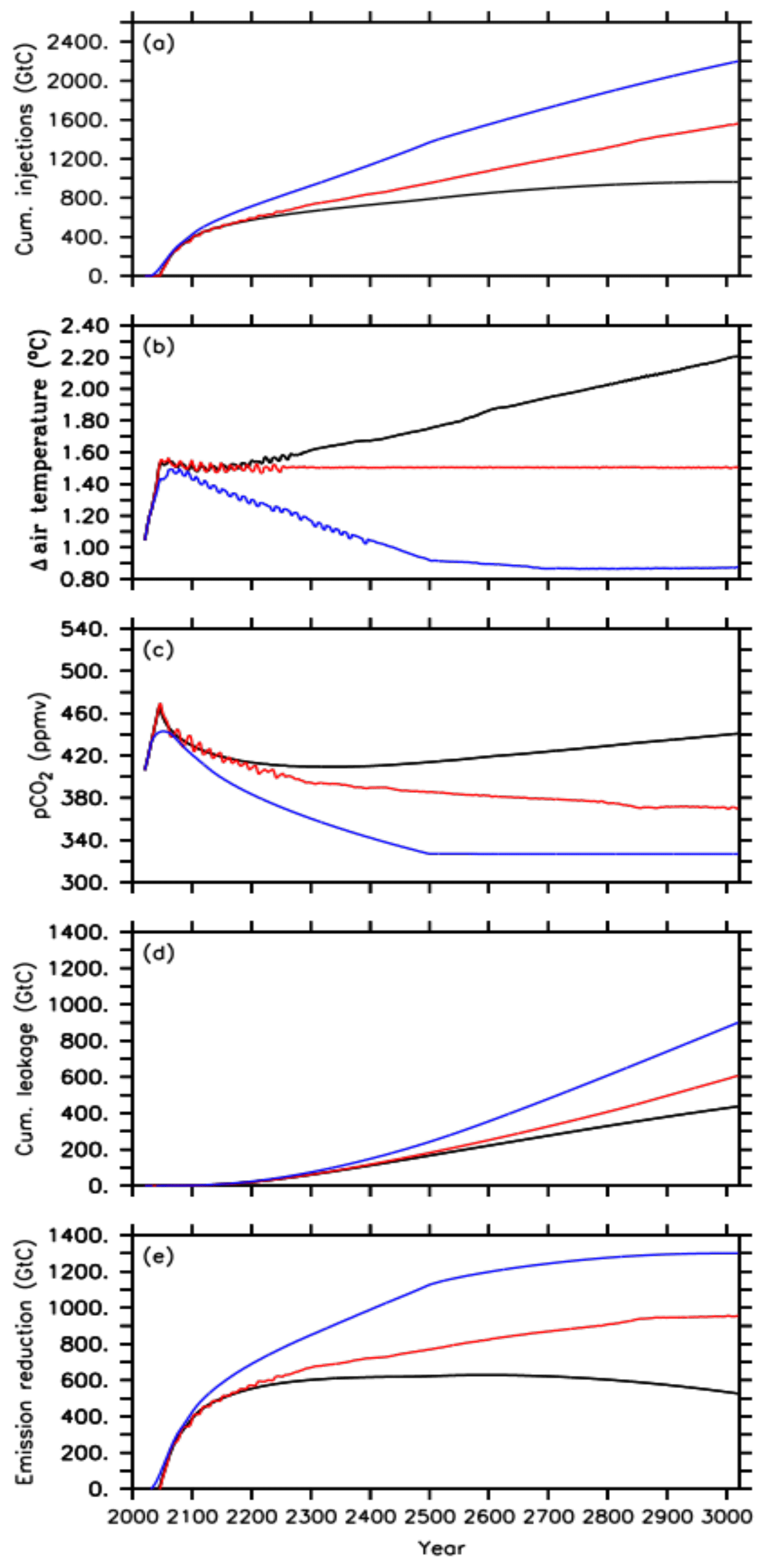
Figure 1 Time series of the different default injection experiments, i.e., the A1 simulation (black lines), A2 simulation (red lines) and A3 simulation (blue lines) for (a) cumulative CO₂ injections, (b) global mean surface air temperature, relative to preindustrial levels, (c) atmospheric CO₂ concentration, (d) cumulative leakage of injected CO₂ and (e) required emission reduction.

2.3 Model experiments

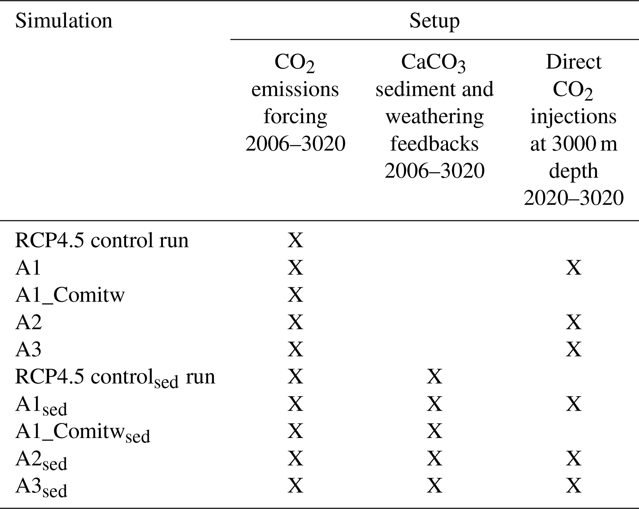
Three conceptually different approaches for applying oceanic CCS are simulated using the UVic model: the first approach (A1) assumes that all anthropogenic CO₂ emissions are injected after a warming of 1.5 ^∘C is realized for the first time; the second approach (A2) injects, in every year, an amount of CO₂ that ensures that temperatures do not rise beyond the 1.5 ^∘C target; and the third approach (A3) injects an amount of CO₂ to ensure that atmospheric CO₂ concentrations follow the RCP/ECP2.6 scenario as closely as possible. All idealized approaches are designed to counter the excessive emissions of the RCP4.5 scenario by direct CO₂ injections into the deep ocean to reach and maintain a specific temperature target as given by the 1.5 ^∘C target until the end of this century and for another millennium. Injections in A2 (A3) are interrupted when the simulated annual mean surface air temperature (atmospheric pCO₂) falls below the respective climate target. We further study how the simulation of CaCO₃ sediment feedbacks and associated continental weathering modifies required CO₂ injections, and the resulting impacts on ocean biogeochemistry are also studied. Table 1 provides an overview of all conducted simulations and their setup from the year 2006 onwards.

Table 1 Overview of all conducted simulations and their setup. The “X” denotes that the respective feature is applied. Note that the applied CO₂ forcing follows the RCP4.5 CO₂ emission scenario from 2006 to 2100 and the extended RCP4.5 CO₂ emissions scenario from 2100 to 2500. From 2500 onwards CO₂ emissions linearly decline until 0 Gt C yr⁻¹ in the year 3020.

In the first approach (A1), all further CO₂ emissions of the RCP4.5 scenario are completely redirected to the injection sites after the global mean surface air temperature has exceeded the 1.5 ^∘C target for the first time. Some committed warming (e.g., Matthews and Caldeira, 2008; Gillet et al., 2011) occurs in these simulations due to past emissions and climate cycle feedbacks. This committed warming is at some point overlaid by the leakage of injected CO₂ out of the ocean (e.g., Orr, 2004; Reith et al., 2016) as well as by oceanic and terrestrial carbon-cycle feedbacks that lead to a CO₂ increase in the atmosphere and respective additional warming (see Sect. 3.1). To diagnose the contribution from leakage, we design a leakage-free sensitivity simulation (A1_Comitw), in which CO₂ emissions are set to zero once the 1.5 ^∘C target is reached, and no CO₂ is injected into the deep ocean.

In contrast to the first approach, the second one (A2) keeps the global mean temperature at the defined threshold of 1.5 ^∘C, relative to preindustrial levels, by injecting as much CO₂ into the deep ocean as is necessary to maintain an annual mean temperature that is only 1.5 ^∘C above preindustrial levels. We diagnose this amount of CO₂ using the transient response to emissions (TCRE, Allen et al., 2009; Matthews et al., 2009; MacDougall, 2016) of our model and the difference of the modeled annual mean atmospheric temperature and the target temperature. CO₂ is only injected if the modeled temperature is above the target temperature. In order to avoid interference with seasonal and longer periodic fluctuations of the atmospheric temperature (sensitivity experiments; not shown), we apply a running-mean-averaging timescale of 1000 d. CO₂ injection rates required to reach the respective target are updated every 5 d, which is when the atmospheric and oceanic model components are coupled. The rate of CO₂ injection taken out of the atmosphere can be larger than the actual CO₂ emissions (RCP/ECP4.5), i.e., constituting net negative CO₂ emissions.

In the third approach (A3), we inject the amount of CO₂ that is needed to follow the atmospheric CO₂ concentrations of the extended Representative Concentration Pathway RCP2.6 and Extended Concentration Pathway ECP2.6, which is a reference scenario that has been suggested to reach the <2 ^∘C climate target with a ≥66 % probability (IPCC, 2014). From the year 2500 onwards, the targeted atmospheric CO₂ concentration is held constant until the end of the simulations. Therefore, at every atmospheric time step the model computes the difference between its currently simulated atmospheric CO₂ concentration, given the RCP4.5 CO₂ emissions, and the targeted atmospheric CO₂ concentration from the RCP2.6 pathway. This difference is used to diagnose the CO₂ injection needed to keep the model's atmospheric CO₂ concentrations as close as possible to the RCP2.6 concentration pathway. A respective amount of CO₂ is injected and subtracted from the prescribed CO₂ emissions to the atmosphere, which eventually results in net negative emissions. We apply temporal averaging and update the required CO₂ injection every 5 d.

In sensitivity experiments (Table 1) we further investigate the effect of CaCO₃ sediment feedbacks and continental weathering on the cumulative CO₂ injections and on seawater carbonate chemistry for the different approaches. The effect of CaCO₃ sediment dissolution is thought to be relevant as CO₂ injected at depth may react relatively directly with sedimentary CaCO₃ and increase CaCO₃ dissolution near or downstream of the injection sites, resulting in an accelerated neutralization of this anthropogenic CO₂ compared to a situation where CO₂ slowly invades the ocean via air–sea gas exchange (Archer et al., 1998; IPCC, 2005). Therefore, we investigate the effect of CaCO₃ sediment feedbacks in our simulations by running the model with and without a sediment sub-model. The global average percentage of CaCO₃ in sediments in our “sed” simulations (Sect. 3.2) is about 31 % for the year 2020 and compares well to about 34.5 % derived from observations as reported in Eby et al. (2009). To ensure that in a steady state (i.e., during the model spin-up) DIC and alkalinity are conserved, the UVic model with the sediment module also has a simple representation of continental weathering to compensate for the burial-related loss of DIC and alkalinity. From the model spin-up we diagnose the global terrestrial weathering flux of DIC as 0.12 Gt C yr⁻¹ with an alkalinity flux of 0.02 Pmol yr⁻¹. During the transient runs with the sediment module, this weathering flux is held constant, whereas sedimentary CaCO₃ accumulation or dissolution is allowed to evolve freely. Consequently, ocean alkalinity and DIC are adjusted in response to interactions between seawater, injected CO₂ and sediments. Simulations with the sediment and weathering sub-model are based on a separate set of spin-up experiments (50 000 years), drift runs and historical simulations that all employ the sediment and weathering sub-model. Hereafter, simulations performed with the sediment and weathering model are referred to by the subscript sed (Table 1).

Relevant carbonate system parameters that are not computed at the model's run-time are derived offline for all simulations by means of the MATLAB version of CO2SYS (Lewis and Wallace, 1998; van Heuven et al., 2009; Koeve and Oschlies, 2012; currently available from http://cdiac.ess-dive.lbl.gov/ftp/co2sys, last access: 17 November 2017), using carbonic acid dissociation constants of Mehrbach et al. (1973), as refitted by Dickson and Millero (1987), and other related thermodynamic constants (Millero, 1995).

3 Results and discussion

3.1 Oceanic CCS and the 1.5 ^∘C climate target

Here, we present the cumulative mass of CO₂ injected in the default runs (without CaCO₃ sediments) of the different approaches and show how effective these are in reaching and maintaining the 1.5 ^∘C climate target.

In the default simulation of the first approach (A1) oceanic CCS starts in the year 2045 after the 1.5 ^∘C climate target has been exceeded for the first time at a corresponding atmospheric CO₂ concentration of about 466 ppmv (Fig. 1a–c). Between the years 2020 and 2045, about 278 Gt C has been emitted in the form of CO₂ into the atmosphere, i.e., a small fraction of the 1242 Gt C of total emissions corresponding to the extended RCP4.5 scenario between the years 2020 and 3020. From 2045 until 3020, all CO₂ emissions (964 Gt C in total) are directly injected into the deep ocean (Fig. 1a), resulting in zero anthropogenic CO₂ emissions into the atmosphere for the remaining simulation. After the injection starts in the year 2045, the atmospheric CO₂ concentration decreases, but this is only until the year 2341, when a minimum of about 409 ppmv is reached (Fig. 1c). The increase of atmospheric CO₂ from year 2342 onwards is a result of an earlier leakage of CO₂ injected into the deep ocean. By the end of the simulation, a total amount of 437 Gt C has leaked back into the atmosphere (Fig. 1d). Thus, only about 55 % of the total mass injected (964 Gt C) remains in the ocean until the year 3020. From 2078 onwards, the land perennially turns into a carbon source with a total carbon loss of about 21 Gt C to the atmosphere.

Global mean temperature, relative to preindustrial levels, oscillates around the 1.5 ^∘C climate target within ±0.02 ^∘C after injections started until the year 2200. Until then, this approach (A1) is thus nearly successful in reaching and maintaining the 1.5 ^∘C climate target. Subsequently, however, global mean surface air temperature shows a slow increase of up to 0.02 ^∘C until 2341 although atmospheric CO₂ is still decreasing. This warming signal is owed to the lagged response of the deep ocean to previously increasing atmospheric CO₂, i.e., committed warming, resulting in a decline of the ocean heat uptake from the atmosphere and thus in an increase of the global mean temperature (Zickfeldt and Herrington, 2015; Zickfeldt et al., 2016). In this simulation (A1), this feedback mechanism (see also Fig. S1 in the Supplement) is overlaid by increasing an leakage of injected CO₂ back into the atmosphere, which becomes the dominating process for atmospheric warming as obvious from the atmospheric CO₂ increase after the year 2342 (Fig. 1c and d). Hence, the global mean air temperature shows a steeper increase until it reaches a maximum of about +2.2 ^∘C above the preindustrial level at the end of the simulation (Fig. 1b). Thus, on a millennial timescale, the A1 simulation overshoots the 1.5 ^∘C climate target by about 0.7 ^∘C. By subtracting this diagnosed leakage of 437 Gt C from the cumulative CO₂ injections (964 Gt C), we determine the required CO₂ emission reduction (527 Gt C) (Fig. 1e) relative to the RCP/ECP4.5 scenario to comply with a global mean temperature of about +2.2 ^∘C, relative to preindustrial levels, on a 1000-year timescale.

Oceanic CCS in the second approach (A2) starts as well in 2045 (Fig. 1a and c). Global mean temperature oscillates around the 1.5 ^∘C climate target until the year 2300 (Fig. 1b). These oscillations get smaller over time until the global mean temperature essentially stays at 1.5 ^∘C until the end of the simulation. We find that the oscillations arise in the applied model from climate–sea-ice feedbacks under the near-term 1.5 ^∘C conditions (see Fig. S2). The terrestrial biosphere turns into a carbon source in 2061 and land–atmosphere carbon fluxes oscillate around zero until the end of the simulation. The total carbon loss from land to the atmosphere is about 75 Gt C. Atmospheric CO₂ concentrations show a continuous decline when the global mean temperature is held at the aspired climate target (Fig. 1b and c). This is caused by a decline in ocean heat uptake as mentioned above and is consistent with an additional accumulation of heat in the atmosphere at constant atmospheric CO₂ concentrations (e.g., Zickfeldt and Herrington, 2015; Zickfeldt et al., 2016). In our second approach, this needs to be counteracted by further CO₂ injections into the deep ocean.

By the end of the A2 run, cumulative CO₂ injections amount to about 1562 Gt C, which is about 600 Gt C (62 %) higher than in the A1 simulation. This amount of additional CO₂ injections is needed in order to reduce global mean warming at the end of the 1000-year simulation from 2.2 ^∘C in A1 to 1.5 ^∘C in A2. In the A2 run, the diagnosed mass of injected CO₂ that has leaked into the atmosphere and has been reinjected into the deep ocean during the entire simulation adds up to about 60 Gt C until the year 3020 (Fig. 1d). Hence, about 61 % of the total mass injected (1562 Gt C) stays in the ocean. This results in a required CO₂ emission reduction of about 955 Gt C (Fig. 1e), i.e., the amount of emission reduction necessary to comply with the 1.5 ^∘C climate target on a 1000-year timescale.

In the third approach, A3, oceanic CCS starts in the year 2031 (Fig. 1a) as the atmospheric CO₂ concentration caused by the RCP4.5 CO₂ emission scenario starts to exceed the targeted RCP2.6 atmospheric CO₂ concentration. Relative to preindustrial levels, the global mean temperature continues to increase to a maximum of approximately +1.5 ^∘C in the year 2078 at a corresponding atmospheric CO₂ concentration of 433 ppmv (Fig. 1b and c). Subsequently, the temperature decreases until it reaches about +0.9 ^∘C relative to preindustrial temperatures, while the atmospheric CO₂ concentration reaches 327 ppmv at the end of the simulation (Fig. 1b and c). Up to that point in time, cumulative CO₂ injections in the A3 simulation amount to about 2200 Gt C (Fig. 1a). In response to negative emissions the land turns into an atmospheric carbon source (Keller et al., 2018) between 2076 and 2600 with a total loss of about 144 Gt C to the atmosphere. From the year 2600 onwards, the carbon flux between the atmosphere and land is nearly zero (below 0.03 Gt C yr⁻¹). By the end of the simulation, the diagnosed leakage of injected carbon adds up to about 900 Gt C (Fig. 1d), which means that about 59 % of the injected CO₂ remains in the ocean until the year 3020. The required emission reduction to move from an RCP4.5 pathway to RCP2.6 in the A3 run is about 1300 Gt C (Fig. 1e).

By the end of the A3 simulation, cumulative CO₂ injections are about 636 Gt C (29 %) higher than in the A2 simulation. This is also reflected in the higher diagnosed leakage by about 293 Gt C in total, when compared to the A2 simulation. In an attempt to follow the atmospheric CO₂ concentration of the RCP2.6 (Sect. 2.3), cumulative CO₂ injections are almost twice the amount of the cumulative CO₂ emissions difference between the RCP4.5 scenario and the RCP2.6 scenario applied here. This can be explained by the fact that deep-oceanic CCS steepens the surface-to-deep DIC gradient (Fig. S3a) fostering a back transport to the surface ocean. Most of this enhanced deep water DIC is transported with the meridional overturning circulation to the Southern Ocean (south of 40^∘ S), where the largest fraction of the total leakage occurs in our injection experiments (Fig. S3b). By the end of the A1 simulation, we find that about 60 % of the diagnosed leakage has outgassed in the Southern Ocean compared to about 77 % in the A2 run and about 80 % in the A3 simulation. Overall, we find that the higher the direct CO₂ injections into the deep ocean are, the higher the leakage (Fig. 1a and d) is and the higher the relative portion outgassed in the Southern Ocean is.

What this means in terms of the effectiveness of oceanic CCS is further highlighted by the comparison of the required cumulative CO₂ injections of the three different approaches (A1, A2 and A3) and the respective required emission reductions needed to reach the run's specific climate target under a RCP/ECP4.5 CO₂ emission scenario. As illustrated in Fig. 2a–c, the approaches A1, A2 and A3 represent increasingly stringent climate targets as evident from decreasing atmospheric warming relative to preindustrial conditions. Cumulative CO₂ injections by the year 2100 are largely equivalent to the required emission reduction because only a tiny fraction of injected CO₂ has outgassed until that point in time (Figs. 1d and 2a). However, by the end of the millennial injection experiments, cumulative CO₂ injections are much larger than the required emission reductions in the year 3020 as indicated by the slopes of the eye-fitted lines in Fig. 2b and c. This is due to the fact that the leakage in the injection experiments (Fig. 1d) requires a larger CO₂ removal effort; i.e., CO₂ that leaks out has to be reinjected. If there were no leakage of injected carbon, i.e., perfect storage, then the cumulative CO₂ injections would equal the required emission reductions.

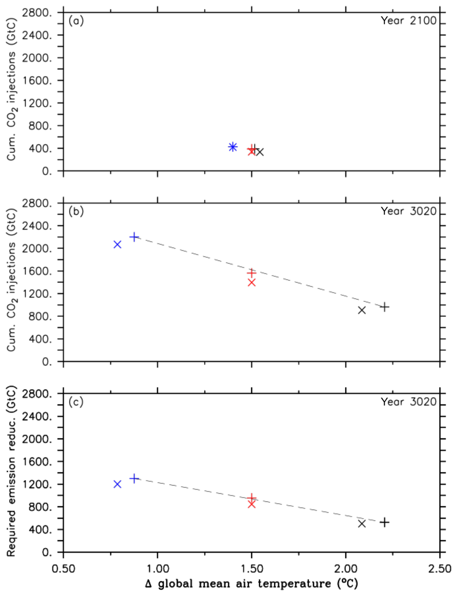
Figure 2 Comparison between simulations of the first approach (A1, black symbols), simulations of the second approach (A2, red symbols) and simulations of the third approach (A3, blue symbols). The cross symbols refer to the default simulations, and the X symbols denote simulations with CaCO₃ sediment and weathering feedbacks. These symbols represent (a) cumulative CO₂ injections and their corresponding global mean temperatures, relative to preindustrial levels, in the year 2100, (b) cumulative CO₂ injections and their corresponding global mean temperatures, relative to preindustrial levels, at the end of the simulation (in the year 3020), and (c) required emission reduction and its corresponding global mean temperature, relative to preindustrial levels, at the end of the simulations. Note that the dashed black lines are eye-fitted to the results of the standard runs.

Land response

Biological processes primarily control the exchange of atmospheric CO₂ with the land, where the majority of the carbon is stored in soils and permafrost. CO₂ is removed from the atmosphere by plant photosynthesis and primarily returned to the atmosphere by respiration and other processes such as fire (Ciais et al., 2013). As long as primary production (GPP; i.e., gross photosynthetic carbon fixation) is greater than carbon losses due to respiration and processes such as fire, the land will be a carbon sink (Le Quéré et al., 2016). If this balance changes, then the land can become a source of CO₂ to the atmosphere. In our simulations as emissions increase and decrease (with oceanic CCS), eventually reaching net negative – and/or zero – emissions, the terrestrial carbon cycle is perturbed and can switch from a sink to a source. The magnitude of the land carbon-cycle response due to an injection-related atmospheric carbon reduction, and an eventual increase as in the A1 experiment (see Sect. 3.1), is mainly governed by the reduced CO₂ fertilization effect on net primary productivity and the temperature-related change in heterotrophic soil respiration, responses that were investigated in Reith et al. (2016). In all simulations the land changes from a carbon sink to source, eventually reaching almost a balance (almost zero net flux) in the A2 and A3 simulations. In the A1 simulation, the increase in atmospheric CO₂ after a period of decline (Fig. 1c) is not able to overcome the temperature effect that elevates respiration rates, and the land continues to perennially lose carbon.

3.2 Sensitivities to CaCO₃ sediment feedbacks and weathering fluxes

As illustrated in Fig. 2b, cumulative CO₂ injections in the A2_sed simulation are about 165 Gt C (11 %) smaller until the year 3020 when compared to the A2 run (1562 Gt C). This smaller CO₂ injection is a result of two processes (CaCO₃ sediment dissolution and constant terrestrial weathering), which both have the net effect of adding alkalinity to the model ocean when compared to the standard experiments without sediment feedbacks and continuous weathering fluxes. By the end of the simulation, average ocean alkalinity has increased by 32 mmol m⁻³ in the A2_sed run compared to an average value of 2422 mmol m⁻³ in the A2 run. About 84 % of this increase in global mean alkalinity can be attributed to ocean CCS and resulting sediment dissolution at depth; the rest is from ocean-acidification-induced CaCO₃ dissolution according to the RCP4.5 CO₂ emission scenario, as evident from the control run with sediment and weathering feedback. An increase in ocean alkalinity may enhance the oceanic uptake of atmospheric CO₂, however, only if waters with increased alkalinity arrive at the surface waters and lower surface ocean pCO₂. This, in turn, reduces the required CO₂ injections to reach and maintain the 1.5 ^∘C climate target. Dissolution of CaCO₃ deep-sea sediments caused by the injection of CO₂ into the deep ocean at 3000 m causes the dissolution of 11.8 Pmol CaCO₃ in the A2_sed simulation by the year 3020, releasing 11.8 Pmol DIC and 23.6 Pmol alkalinity to the deep ocean. Highest CaCO₃ dissolution rates occur in the vicinity of the seven injection sites (Fig. S4a and b). Hence, ocean acidification reaching the deep ocean and ocean CCS convert sediments from a CaCO₃ sink (116 Gt CaCO₃-C at the end of the respective spin-up run) to a source of its dissolution products. A second process that contributes to the increase in ocean alkalinity is the terrestrial CaCO₃ weathering flux, which arrives in the surface ocean via river discharge and amounts to about 19.3 Pmol alkalinity and 9.7 Pmol C (116 Gt C) by the end of the A2_sed simulation.

Disentangling the relative role of the two processes (turning CaCO₃ burial into CaCO₃ dissolution and the continuous flux of alkalinity from terrestrial weathering) with respect to stabilizing oceanic CO₂ uptake and thereby affecting the required CO₂ injections is not trivial. Waters affected by CaCO₃ sediment dissolution in the deep ocean need to return to the ocean surface before having an effect on surface ocean pCO₂ and oceanic CO₂ uptake (Cao et al., 2009). The fluxes from terrestrial weathering, however, are in our simulation, continuous and constant with time (no sensitivity to weathering changes in atmospheric pCO₂, surface air temperature, precipitation or terrestrial production) and directly arrive in the surface ocean via river inflow. It is thus likely that, in comparison to the standard experiments without terrestrial weathering, the latter affects the atmosphere–ocean CO₂ flux well before the alkalinity input related to CaCO₃ dissolution. Quantifying the effect of each process to reduce the required CO₂ injection individually, however, would require additional simulations, e.g., experiments with CaCO₃ dissolution turned on but terrestrial weathering turned off. This is beyond the scope of this study. As a consequence of the two processes mentioned above, the required emission reduction amounts to about 846 Gt C, i.e., ∼109 Gt C (11 %) less when compared to the A2 run (Fig. 2b).

The net effects of sediment and weathering feedbacks on the required CO₂ injections in simulations of the second approach described above are as well represented in the injection experiments of the first and third approach, but they are of a smaller magnitude, i.e., 5 % less (Fig. 2a–c).

3.3 Biogeochemical impacts

Here, we present injection-related biogeochemical impacts with respect to changes in pH and the saturation state of aragonite in the default simulations of the second (A2) and third approach (A3) and of the respective RCP4.5 control run. Simulations of the first approach are neglected here because this one cannot reach and maintain the 1.5 ^∘C climate target.

At the beginning of our default simulations (in the year 2020), the uptake of anthropogenic CO₂ has lowered average pH at the ocean surface by about 0.12 units, relative to its preindustrial value of about 8.16 (Fig. 3a). This trend continues in the control simulation until its maximum reduction of about −0.25 units in the year 2762, which stays nearly constant until the end of the simulation (Fig. 3a).

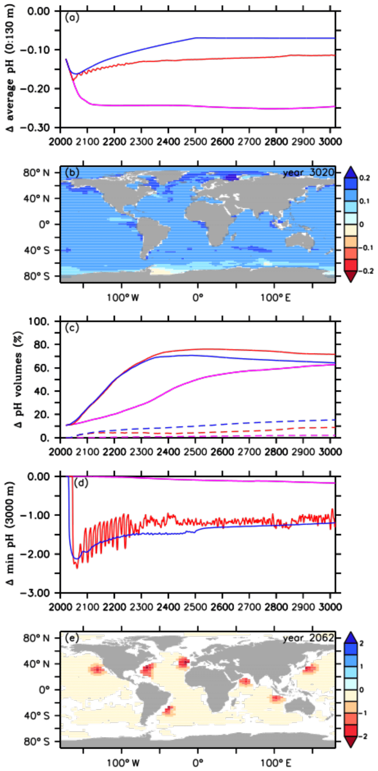
Figure 3 Comparison of pH values between the default RCP4.5 control run (purple lines), the A2 simulation (red lines), and the A3 simulation (blue lines) for (a) the average ocean surface pH (0 to 130 m depth), (b) the difference in ocean surface pH, relative to preindustrial levels, between the A2 simulation and the default RCP4.5 control run in the year 3020, (c) pH volumes of the first (≤7.8 and ≥7.4, solid lines) and second categories (<7.4, dashed lines), (d) minimum pH values at 3000 m depth, and (e) the difference in minimum pH at 3000 m depth between the A2 simulation and the default RCP4.5 control run in the year 2062.

As direct CO₂ injections lead to a decline in the atmospheric CO₂ concentration (Fig. 1c) and, in consequence, to a lower upper-ocean carbon uptake via air–sea gas exchange, we find smaller reductions in the average ocean surface pH, i.e., reduced upper-ocean acidification, after the year 2045 in the A2 simulation and after the year 2031 in the A3 run (Fig. 3a), i.e., shortly after their respective oceanic CCS starting points (Fig. 1a). In the year 3020 the average ocean surface pH in the A2 simulation is about +0.13 units higher, when compared to the control run (Fig. 3a). Using global mean surface ocean pH as a metric, surface ocean acidification in the year 3020 compared to the year 2020 is slightly more intense in the A2 simulation but even more reduced in the A3 run. In both cases this is a direct effect of a lower atmospheric pCO₂ (Fig. 1c) compared to the year 2020. Amelioration of surface ocean pH shows regional variability (Fig. 3b), with local maxima of the pH difference between the A2 simulation and the control run in the year 3020 up to +0.23 units, in particular in northern latitudes (Fig. 3b). However, surface ocean acidification is less reduced in the Southern Ocean and even slightly higher in parts of the Weddell Sea, where most of the injected CO₂ leaks back into the atmosphere (Fig. 3b).

The simulated ameliorations in the surface ocean pH come at the expense of strongly acidified water masses in the vicinity of the seven injection sites at 3000 m depth, when compared to the RCP4.5 control run. In order to assess how much of the global ocean volume ($\sim \mathrm{1.6}\times {\mathrm{10}}^{\mathrm{9}}$ km³) shifts to biotically critical pH values in our simulations, we define two pH categories. The first category is defined as 7.4 ≤ pH ≤ 7.8 (solid lines in Fig. 3c) and is chosen because studies have shown that all calcifiers such as coralline algae and foraminiferans are strongly reduced or are absent from acidified areas (pH < 7.8), and the overall biomass of the benthic community is about 30 % less compared to normal conditions (e.g., IPCC, 2011; Fabricius et al., 2015). The second category includes pH values that are lower than 7.4 (dashed lines in Fig. 3c). Such low pH values are for instance found in the vicinity of volcanic CO₂ vents and cause a massive drop in biodiversity (e.g., Ogden, 2013).

In our control simulation, we find a steady increase in the ocean volume characterized by 7.4 ≤ pH ≤ 7.8, from about 11 % of total ocean volume in the year 2020 to about 63 % in the year 3020 (Fig. 3c). Oceanic CCS in the A2 and A3 simulation leads to a much steeper increase of “moderately” acidified waters (7.4 ≤ pH ≤ 7.8) with maximum values of 76 % and 71 %, respectively, in the year 2551 (Fig. 3c), but these decrease to 72 % and 64 % in the year 3020. Considering our chosen category (7.4 ≤ pH ≤ 7.8), ocean CCS mainly speeds up interior-ocean acidification but does not increase the acidified volume at the end of the simulation very much. At the end of the simulation the A3 simulation and the A2 run show an increase of affected interior-ocean water by 1 % and 13 %, respectively, compared to the control run.

Respective volumes of the second category (pH < 7.4) start to appear around the year 2400 in the control simulation and then slowly increase to about 2 % until the end of the simulation (Fig. 3e). In contrast, oceanic CCS directly results in the immediate appearance of waters with pH < 7.4, with a volume steadily increasing until the year 3020, where it reaches 9 % of total ocean volume in the A2 simulation and 15 % in the A3 run (Fig. 3c). The differences in both pH categories between the injection experiments are due to the higher cumulative mass of injected CO₂ in the A3 run, leading to a smaller volume in the first category and to a bigger volume in the second one (Figs. 1a and 2b).

In order to further identify extreme pH values related to the injections, we look at minimum pH values. These are found at 3000 m depth, i.e., the depth at which oceanic CCS is carried out. Relative to preindustrial conditions, the highest reductions in pH minima are found in the A2 simulation with about −2.37 units in the year 2062, however with large regional variability (Fig. 3d and e). Subsequently, the pH minima in the A2 simulation show strong oscillations until about the year 2400, which are caused by the different annual CO₂ injection rates. By the end of the A2 simulation, minimum pH values at 3000 m depth are up to 1 unit lower than in the control run (Fig. 3d). We find a similar pattern in the A3 simulation, although the pH reductions show only slight oscillations, resulting in a more constant pH reduction than in the A2 simulation (Fig. 3d). In comparison to the injection experiments, minimum pH values in the control run start to appear from the year 2300 onwards, leading to a reduction by about −0.17 units in the year 3020 (Fig. 3d); i.e., the deep ocean feels ocean acidification very slowly.

To summarize we observe an increasing benefit in reduced acidification at the ocean surface with higher cumulative CO₂ injections, which comes at the expense of increasing acidified water masses in the intermediate and deep ocean, with the strongest pH reductions in the vicinity of the injection sites (Fig. 3e). Figure 4a and b illustrate this trade-off for the injection experiments of the A2 and A3 simulations as well as for the respective control runs in the year 3020. By comparing the different simulations with each other, we find that continental weathering and CaCO₃ sediment feedbacks lead to a slightly higher increase in average pH levels at the ocean surface as well as smaller minimum pH values at 3000 m depth, when compared to preindustrial levels. This is caused by the dissolution of CaCO₃ sediments and the terrestrial weathering flux, which both have the net effect of adding alkalinity to the ocean and thereby increasing the buffer capacity of seawater.

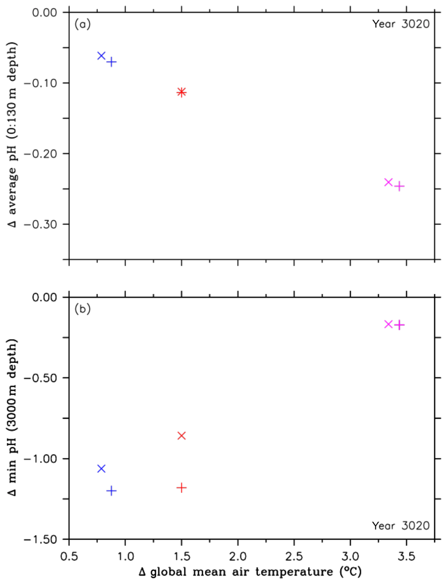
Figure 4 Comparison of pH values and their corresponding global mean temperatures in the year 3020, both relative to preindustrial levels, between the RCP4.5 control simulations (purple symbols), simulations of the second approach (A2, red symbols), and simulations of the third approach (A3, blue symbols). The cross symbols refer to the default simulations, and the X symbols denote simulations with CaCO₃ sediment and weathering feedbacks. These symbols represent (a) changes in the ocean surface pH (0 to 130 m depth), relative to preindustrial levels, and (b) changes in minimum pH values at 3000 m depth, relative to preindustrial levels.

The reported reductions in global average surface pH in our control simulation caused by the partial oceanic uptake of the RCP4.5 CO₂ emissions correspond to an increase in hydrogen ions (H⁺), which partly react with carbonate ions (${\mathrm{CO}}_{\mathrm{3}}^{\mathrm{2}-}$) to form bicarbonate ions (${\mathrm{HCO}}_{\mathrm{3}}^{-}$). This leads in consequence to a reduction in the surface saturation state (Ω) with respect to the CaCO₃ minerals aragonite and calcite. This is of importance to marine calcifiers because the formation of shells and skeletons generally occurs where Ω>1 and dissolution occurs where Ω<1 (unless the shells or skeletons are protected, for instance, by organic coatings) (Doney et al., 2009; Guinotte and Fabry, 2008). Since aragonite is about 1.5 times more soluble than calcite (Mucci, 1983) and since aragonite is the mineral form of coral reefs, which are of large socioeconomic value, we only report here on simulated changes in the saturation state of aragonite.

To investigate how tropical coral reef habitats might be impacted in our simulations, we here define the potential coral reef habitat as the volume of the global upper ocean (0–130 m, the two topmost model grid cells), which is characterized by Ω_AR>3.4 and ocean temperatures between 21 and 28 ^∘C, where most coral reefs exist (Kleypas et al., 1999). We present this volume as the percent fraction of the total upper-ocean volume (4.637×10⁷ km³) in our model.

For preindustrial conditions (in the year 1765), we find that about 37 % of the upper-ocean volume is within our defined thresholds (green star in Fig. 5a and b). At the beginning of our simulations (in the year 2020), this coral reef habitat volume has already declined to about 13 %, consistent with the current observation that many coral reefs are already under severe stress (e.g., Pandolfi et al., 2011; Ricke et al., 2013). In the RCP4.5 control run, we observe that the potential tropical coral reef habitat volume reaches 0 % in the year 2056 and remains so thereafter (Fig. 5a) with a decrease in aragonite oversaturation levels being the main driver.

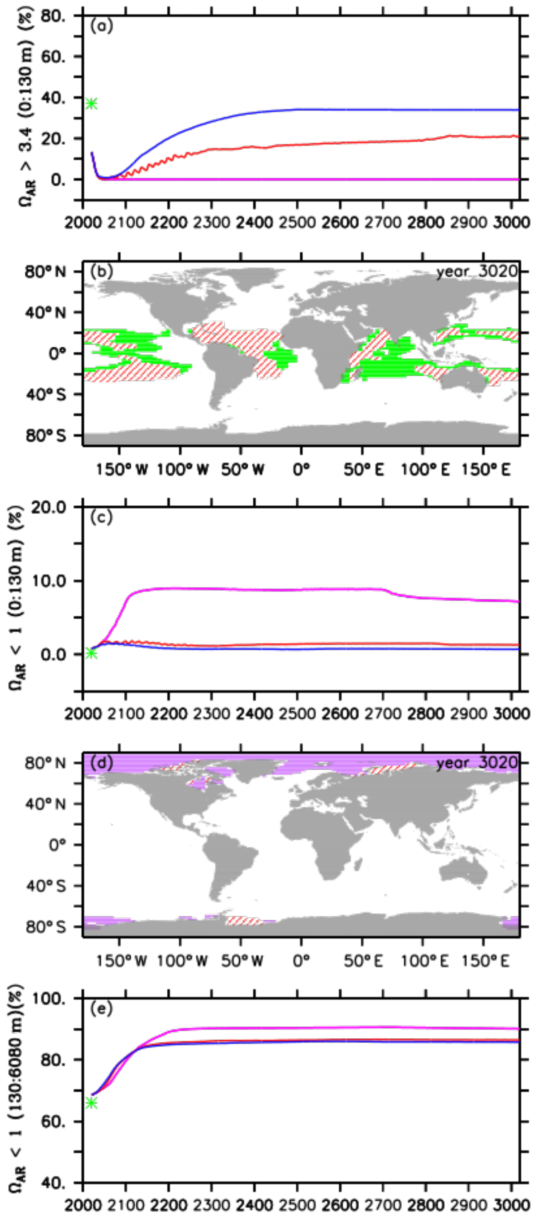
Figure 5 Comparison of volumes for different saturation states between preindustrial levels (green stars), the default RCP4.5 control run (purple lines), the A2 simulation (red lines), and the A3 simulation (blue lines) for (a) omega aragonite > 3.4 in the upper ocean (0 to 130 m depth), (b) potential coral reef habitat defined as the volume of the global upper ocean (0 to 130 m depth) with omega aragonite > 3.4 and ocean temperatures between 21 and 28 ^∘C for preindustrial levels (green) and the A2 simulation (red hatching) in the year 3020, (c) omega aragonite < 1 in the upper ocean (0 to 130 m depth), (d) the global distribution of omega aragonite < 1 for the default control run (purple) and the A2 simulation (red hatching), and (e) omega aragonite < 1 in the intermediate and deep ocean (130 to 6080 m depth).

In our injection experiments, we find an increase in the potential tropical coral reef habitat volume right after the start of oceanic CCS (Fig. 5a). Despite this, in the A2 simulation the respective volume still approaches zero (0.2 %) in the year 2044, although it does then steadily increase again until it reaches 21 % at the end of the simulation, i.e., still 16 % less than its preindustrial state but also 8 % more compared to the current situation (Fig. 5a and b). The respective habitat volume in the A3 simulation shows an earlier and stronger increase, resulting in a habitat volume of about 34 %, i.e., 3 % less than preindustrial levels, at the end of the model experiment (Fig. 5a).

In preindustrial times, water masses in the upper ocean (0–130 m) that were undersaturated with respect to aragonite (Ω_AR<1) were negligible (0.2 %; Fig. 5c, green star). This undersaturated volume has increased to about 1 % at the beginning of our simulations. Over the course of the control run, we observe an increase with a maximum of about 9 % in the year 2212. Subsequently, the respective undersaturated volume slightly decreases until it reaches a minimum of about 7 % at the end of the simulation. Undersaturated surface waters are located in higher latitudes (Fig. 5d), which is, for instance, considered a threat to pteropods like Limacina helicina (e.g., Lischka et al., 2011). In the A2 and A3 simulations, the respective undersaturated volumes are significantly smaller and never exceed 2 % of the surface ocean volume (Fig. 5c and d). Undersaturated surface water volumes in the A2 run are slightly higher than those in the A3 simulation.

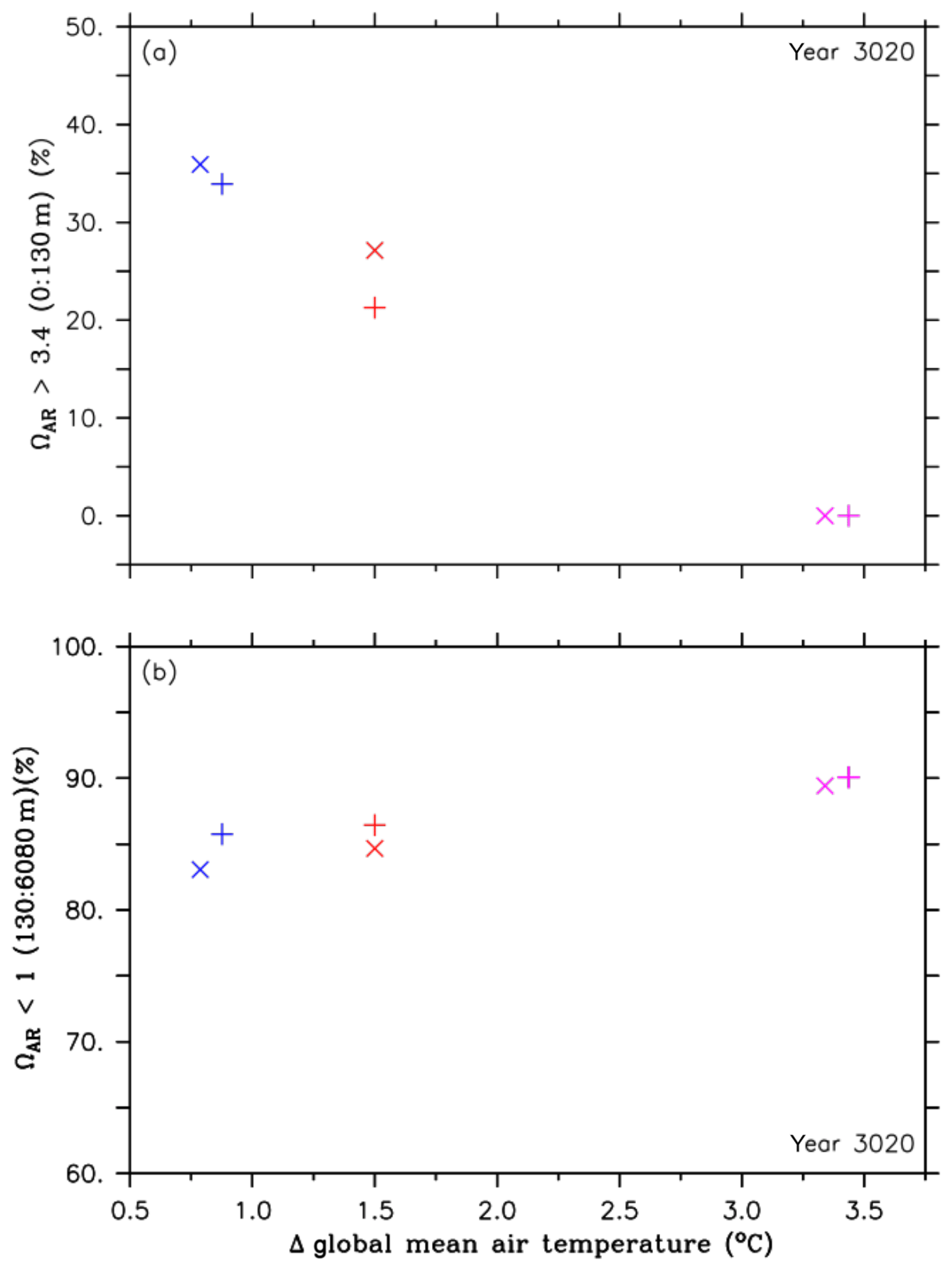
Figure 6 Comparison of volumes for different aragonite saturation states and their corresponding global mean temperatures in the year 3020, both relative to preindustrial levels, between the RCP4.5 control simulations (purple symbols), simulations of the second approach (A2, red symbols) and simulations of the third approach (A3, blue symbols). The cross symbols refer to the default simulations, and the X symbols denote simulations with CaCO₃ sediment and weathering feedbacks. These symbols represent (a) omega aragonite > 3.4 in the upper ocean (0 to 130 m depth), relative to preindustrial levels, and (b) changes in minimum pH values at 3000 m depth, relative to preindustrial levels.

Further, we assess the volume that is undersaturated with respect to aragonite in the intermediate and deep ocean (130–6080 m) and present it as a percentage of the entire interior-ocean volume (1.311×10⁹ km³). This is of interest since changes in interior-ocean Ω_AR may affect the growth conditions of cold-water corals (e.g., Guinotte and Fabry, 2008; Flögel et al., 2014; Roberts and Cairns, 2014) and the dissolution depth of sinking aragonite particles.

At the beginning of the simulations, 69 % of the interior oceans are undersaturated with respect to aragonite, which is about 3 % more than preindustrial levels (Fig. 5e). Subsequently, the increase in undersaturated water volume is similar among all simulations until about the year 2122, when the undersaturated volume in the control simulation continues to increase until its maximum of about 91 % in the year 2713. The undersaturated volumes in the injection experiments show only a very small increase after the year 2122, leading until the year 3020 to values of about 86 % in both injection simulations (Fig. 5e). The bigger volume in the control run is likely caused by acidified waters at the ocean surface that ventilate intermediate and mode waters (Resplandy et al., 2013).

Figure 6a and b show a similar trade-off in the injection experiments of the second and third approach in the year 3020 regarding pH (Fig. 4a and b), i.e., an increase of the aragonite saturation states in the upper ocean and an increase of undersaturated conditions in the intermediate and deep ocean. Further, the effects of CaCO₃ sediment dissolution and continental weathering lead to the highest benefit in the upper ocean and the lowest harm in the intermediate and deep ocean (Fig. 6a and b). See Sect. 1 and Figs. S5–S9 about the different evolution of the aragonite saturation horizon (Ω_AR=1, ASH) in the RCP4.5 control run and the A2 and A3 experiments.

As mentioned in the introduction, the neglect of non-CO₂ greenhouse gases in our injection experiments underestimates the required cumulative CO₂ injections and associated trade-offs in each approach. This is due to the fact that non-CO₂ greenhouse gases directly affect the Earth's energy balance, resulting in either warming or cooling of the atmosphere. Gases like methane and nitrous oxide warm the Earth, while aerosols such as sulfate cool it (e.g., Myhre et al., 2013). The current net effect is a small positive radiative forcing, which, although controversially debated, is expected to increase as the cooling effect of sulfate aerosols is predicted to decline over the next half of this century (Moss et al., 2010; Hansen et al., 2017; Rao et al., 2017).

4 Conclusion

This modeling study explores the potential and biogeochemical impacts of three different approaches to control the amount of oceanic CCS as a means to fill the gap between the CO₂ emissions and climate impacts of the RCP4.5 scenario and a specific temperature target such as the 1.5 ^∘C climate target. We do so from the perspective of using only ocean CCS for this purpose.

The analysis of the A1 simulation (first approach) reveals that because of committed warming and the eventual outgassing of some of the injected CO₂, it would not be sufficient to inject the residual RCP4.5 CO₂ emissions (964 Gt C in total) once a global mean temperature of 1.5 ^∘C is exceeded for the first time (in the year 2045) until the year 3020. In order to overcome the observed overshoot of +0.7 ^∘ C by the year 3020 in the first approach, we find that about 600 Gt C (62 %) more needs to be injected, as indicated by the default simulation of the second approach, i.e., the A2 run (Figs. 1a, b and 2b).

Following the atmospheric CO₂ concentration of the RCP/ECP2.6 as closely as possible by applying oceanic CCS would require cumulative CO₂ injections of about 2200 Gt C until the year 3020. However, global mean temperature reaches +0.9 ^∘C by the end of the A3 simulation and thus undershoots the respective climate target.

The cumulative CO₂ injections in the second and third approach and the respective required emission reductions question the suitability of oceanic CCS for the aspired target on such a timescale because the outgassed CO₂ amounts, which are 607 and 900 Gt C by the year 3020, respectively (Figs. 1d and 2b, c), would need to be recaptured by additional technologies such as direct air capture and subsequently reinjected into the deep ocean. The required emission reductions of about 955 Gt C in the second approach and about 1300 Gt C in the third approach point to the massive CO₂ amounts that would need to get removed from the atmosphere under the RCP/ECP4.5 CO₂ emission scenario in order to be compatible with the 1.5 ^∘C or lower climate target on a millennium timescale.

From the integrated analysis of the model runs from all three approaches (i.e., eye-fitted lines in Fig. 2b and c), we quantify the amount of emission reduction and oceanic CCS, respectively, required to lower the model-predicted global mean temperature by 1 ^∘C. In the near future (2100) this measure is 446 Gt C ^∘C⁻¹ for both oceanic CCS and the required emission reductions as only a tiny fraction has outgassed until that point in time (see Sect. 3.1). On a millennial timescale this measure is about 951 Gt C ^∘C⁻¹ for oceanic CCS and about 595 Gt C ^∘C⁻¹ (37 % less) for the required emission reductions, respectively, highlighting that a large fraction of injected CO₂ has outgassed.

Inclusion of CaCO₃ sediment and weathering feedbacks reduces the required cumulative CO₂ injections and required emission reductions by about 6 % in the first and third approach and by about 11 % in the second approach, respectively (Fig. 2b and c). The neglect of non-CO₂ greenhouse gases in the applied forcing of the injection experiments underestimates the cumulative CO₂ injections that would be required. In general, it is estimated that non-CO₂ climate agents contribute between 10 % and 30 % to the total forcing (Friedlingstein et al., 2014) until the year 2100 and for business-as-usual simulations. Extrapolating the current contribution of greenhouse gases other than CO₂ qualitatively into the future, we expect that CO₂ injections of the magnitude of the A3 simulation may be required to stay safely below +1.5 ^∘C on a millennium timescale. We propose that our generalized estimates of emission reduction and oceanic CCS per 1 ^∘C cooling, respectively, may be used in the future to quantify additional efforts in order to compensate for non-CO₂ greenhouse-gases-induced warming.

With respect to the biogeochemical impacts in the injection simulations of the second and third approach, we observe an increase of the average pH and aragonite saturation states in the surface ocean (0–130 m) after the start of oceanic CCS, when compared to the RCP4.5 control run. These are due to the direct effect of a lower atmospheric pCO₂ in the injection experiments, i.e., reduced upper-ocean acidification (Sect. 3.3).

Potential tropical coral reef habitats in the upper-ocean volume, which are here defined as having an Ω_AR>3.4 and ocean temperatures between 21 and 28 ^∘C, are observed to steadily increase after the start of oceanic CCS in the A2 run and the A3 simulation (Fig. 5a), almost reaching preindustrial levels in the A3 simulation. However, the potential coral reef habitats in the respective injection experiments are close to zero for several decades (Fig. 5a), raising the question of whether coral reefs would be able to recover from globally inhabitable conditions after this period of time. Local application of ocean alkalinization (Feng et al., 2016) may be a technical solution to protect coral reefs during this time period, in particular in regions where coral reefs are essential for shoreline protections.

The observed reduction of ocean acidification in the surface ocean comes at the expense of more strongly acidified water masses in the intermediate and deep ocean, with the strongest reductions in pH levels in the vicinity of the seven injections sites (Fig. 3d and e). Although it is difficult to predict how this would impact marine ecosystems, it is very likely that such conditions would put them under severe stress.

Overall, the trade-off between injection-related damages in the deep ocean and benefits in the upper ocean illustrate the challenge of evaluating the offset of local harm against global benefit, which is very likely the subject of any deliberate CO₂ removal method (e.g., Smith et al., 2016; Boysen et al., 2017; Fuss et al., 2018). Leaving aside the massive economic effort associated with ocean CCS of the size needed to reach the 1.5 ^∘C climate target (even when starting from a currently optimistic RCP4.5 mitigation scenario), humanity will have to decide whether severe stress and potential loss of deep-sea ecosystems is acceptable when paid off by conserving or restoring surface ocean ecosystems to a large extent.