Investigating the applicability of emergent constraints

Recent research on emergent constraints (ECs) has delivered promising results in narrowing down uncertainty in climate predictions. The method utilizes a measurable variable (predictor) from the recent historical past to obtain a constrained estimate of change in an entity of interest (predictand) at a potential future CO₂ concentration (forcing) from multi-model projections. This procedure first critically depends on an accurate estimation of the predictor from observations and models and second on a robust relationship between inter-model variations in the predictor–predictand space. Here, we investigate issues related to these two themes in a carbon cycle case study using observed vegetation greening sensitivity to CO₂ forcing as a predictor of change in photosynthesis (gross primary productivity, GPP) for a doubling of preindustrial CO₂ concentration. Greening sensitivity is defined as changes in the annual maximum of green leaf area index (LAI_max) per unit CO₂ forcing realized through its radiative and fertilization effects. We first address the question of how to realistically characterize the predictor of a large area (e.g., greening sensitivity in the northern high-latitude region) from pixel-level data. This requires an investigation into uncertainties in the observational data source and an evaluation of the spatial and temporal variability in the predictor in both the data and model simulations. Second, the predictor–predictand relationship across the model ensemble depends on a strong coupling between the two variables, i.e., simultaneous changes in GPP and LAI_max. This coupling depends in a complex manner on the magnitude (level), time rate of application (scenarios), and effects (radiative and/or fertilization) of CO₂ forcing. We investigate how each one of these three aspects of forcing can affect the EC estimate of the predictand (ΔGPP). Our results show that uncertainties in the EC method primarily originate from a lack of predictor comparability between observations and models, the observational data source, and temporal variability of the predictor. The disagreement between models on the mechanistic behavior of the system under intensifying forcing limits the EC applicability. The discussed limitations and sources of uncertainty in the EC method go beyond carbon cycle research and are generally applicable in Earth system sciences.

1 Introduction

Earth system models (ESMs) are powerful tools to predict responses to a variety of forcings such as an increasing atmospheric concentration of greenhouse gases and other agents of radiative forcing (Klein and Hall, 2015). Still, long-term ESM projections of climate change have substantial uncertainties. This can be due to poorly understood processes in some cases and to missing or simplified representations called parameterizations in others (Flato et al., 2013; Klein and Hall, 2015; Knutti et al., 2017). Certain important processes, especially in the atmosphere, happen at spatial scales finer than can possibly be represented in current ESMs. Consequently, various phenomena in the system ranging from local extreme precipitation events to large-scale climate modes can be poorly simulated (Flato et al., 2013). Errors propagate and can be amplified through feedbacks among interacting components in the Earth system, resulting in biases whose origins can be difficult to identify (Flato et al., 2013). Furthermore, an inherent component of the Earth climatic system, its internal natural variability, is complicated to represent and simulate in models (Flato et al., 2013; Klein and Hall, 2015).

Model intercomparison projects explore these uncertainties by coordinating a wide range of simulation setups focusing on internal variability, boundary conditions, and parameterizations (Taylor et al., 2012; Flato et al., 2013; Eyring et al., 2016; Knutti et al., 2017). Models developed at various institutions are driven with the same forcing information (e.g., historical forcing) or with identical idealized boundary conditions. However, each modeling group decides which of the processes to consider and implement in their ESM. The conventional approach of handling these multi-model ensembles is to use unweighted ensemble averages (Knutti, 2010; Knutti et al., 2017). This assumes that the models are independent of one another and equally good at simulating the climate system (Flato et al., 2013; Knutti et al., 2017). The large spread between model projections suggests that this assumption is not valid. Therefore, alternate methods have been developed to extract results more accurate than multi-model averages (e.g., model weighting scheme based on performance and interdependence; Knutti et al., 2017). The concept of emergent constraints arises in this context, namely as a method to reduce uncertainty in ESM projections relying on historical simulations and observations (Hall and Qu, 2006; Boé et al., 2009; Cox et al., 2013; Klein and Hall, 2015; Cox et al., 2018).

The two key parts of a method based on emergent constraint (EC) are a linear relationship arising from the collective behavior of a multi-model ensemble and an observational estimate for imposing the said constraint (Fig. 1). The linear relationship is a physically (or physiologically) based correlation between inter-model variations in an observable entity of the contemporary climate system (predictor) and a projected variable (predictand) that is difficult to observe or not observable at all. Combining the emergent linear relationship with observations of the predictor sets a constraint on the predictand (Cox et al., 2013; Flato et al., 2013; Klein and Hall, 2015; Knutti et al., 2017). Many such ECs have been identified and reported, as briefly summarized below.

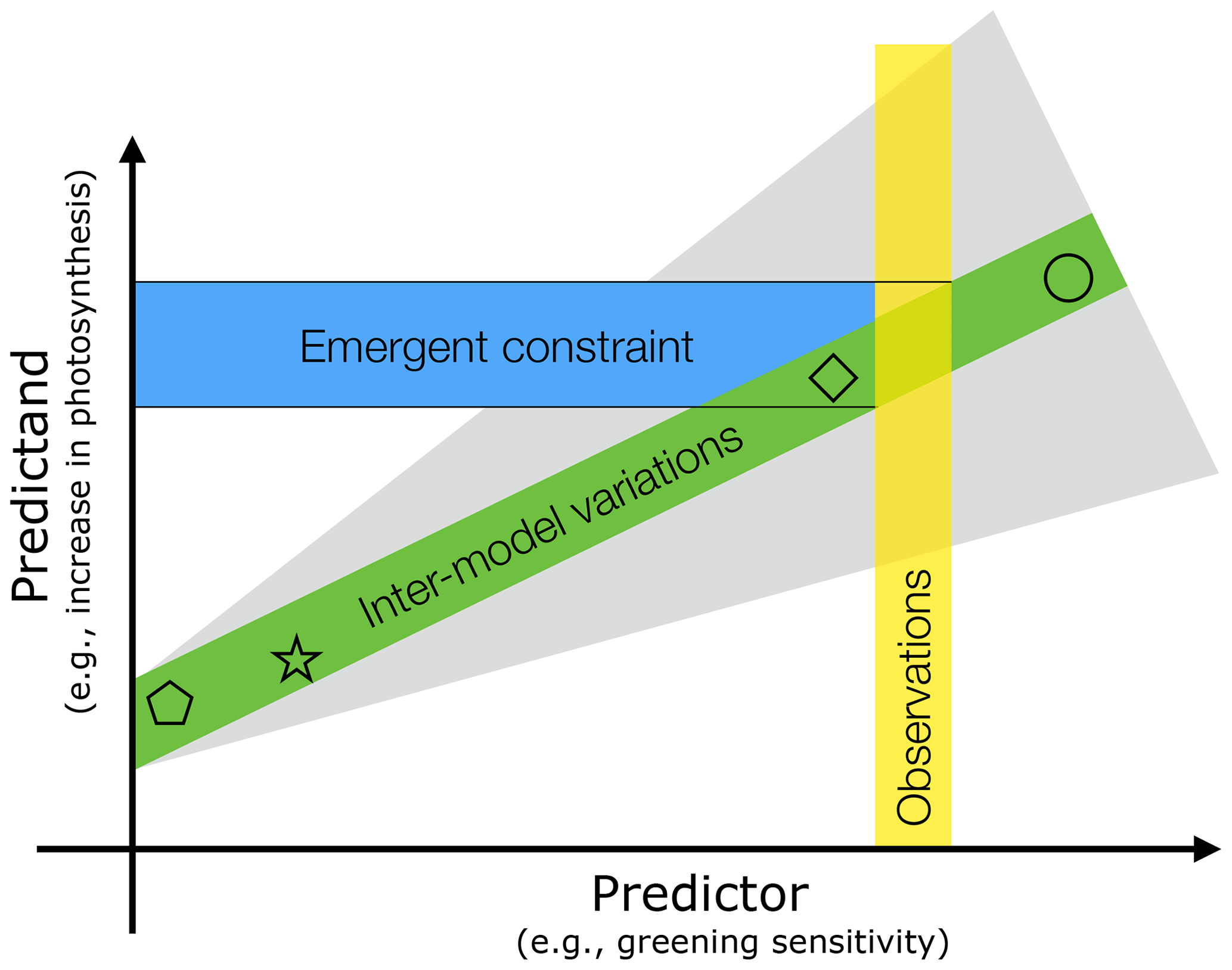
Figure 1 Schematic depiction of the emergent constraint (EC) method and factors affecting the uncertainty of the constrained estimate. The predictor (x axis) is change in the annual maximum of green leaf area index (LAI_max) due to unit forcing (CO₂ increase and associated climatic changes) during a representative historical period. It is termed greening sensitivity in this study. The predictand (y axis) is projected change in gross primary productivity (GPP) in response to rising CO₂ concentration (e.g., for a doubling of the preindustrial level). Both the predictor and predictand refer to large area values: in this case, the entire northern high latitudes (NHLs). Inter-model variations (each symbol represents a model) in matching pairs of predictors and predictands result in a linear relationship between the two (green band); i.e., the ratio (predictand ∕ predictor) is approximately constant across the model ensemble. The slope depends on forcing attributes (gray shading), such as its level (CO₂ concentration; Sect. 3.4), time rate of application (scenarios such as various RCPs; Sect. 3.4), and different effects (i.e., fertilization, radiative forcing; Sect. 3.5). The observed sensitivity (vertical yellow bar) is used to find the constrained estimate of the predictand (i.e., change in GPP). The ability to accurately estimate the predictor depends on the source of observational data (Sect. 3.1) and its spatial (Sect. 3.2) and temporal variability (Sect. 3.3). Observed (yellow bar) and modeled predictor values (x coordinate of symbols) must be obtained from matching time periods, i.e., at the same level of historical forcing, to ensure comparability (Sect. 3.3 and 3.4). All these factors, together with the goodness of fit of inter-model variations (width of green shading), finally define the uncertainty of the derived constrained estimate (blue horizontal bar with black solid lines depicting the upper and lower bound of uncertainty).

Hall and Qu (2006) proposed a constraint on projections of snow albedo the feedback based on the correlation between large inter-model variations in feedback strength of the current seasonal cycle. The EC was first established for the CMIP3 ensemble and confirmed for phase five of the Coupled Model Intercomparison Project (CMIP5; Flato et al., 2013; Qu and Hall, 2014). Several EC studies followed with the goal of reducing uncertainty in projections of the cloud feedback under global warming, as reviewed by Klein and Hall (2015). It is thought that erroneous representation of low-cloud feedback in ESMs essentially contributes to the large uncertainty in equilibrium climate sensitivity (ECS; 1.5 to 5 K), i.e., warming for a doubling of preindustrial atmospheric CO₂ concentration (2×CO₂; Sherwood et al., 2014; Klein and Hall, 2015). Recently, Cox et al. (2018) presented a different approach to constrain ECS based on its relationship to the variability of global temperatures during the recent historical warming period. They reported a constrained ECS estimate of 2.8 K for 2×CO₂ (66 % confidence limits of 2.2–3.4 K).

The concept of EC also found its way into the field of carbon cycle projections. A series of studies analyzed the extent to which interannual atmospheric CO₂ variability can serve as a predictor of the long-term temperature sensitivity of terrestrial tropical carbon storage. Cox et al. (2013) and Wenzel et al. (2014) reported an emergent linear relationship, although with different slopes for CMIP3 and CMIP5 ensembles, resulting in slightly divergent constrained estimates (CMIP3: $-\mathrm{53}\pm \mathrm{17}$ Pg C K⁻¹, CMIP5: $-\mathrm{44}\pm \mathrm{14}$ Pg C K⁻¹). Wang et al. (2014), however, were unable to detect a similar relationship between the proposed predictor and predictand. Recently, Lian et al. (2018) presented an EC estimate of the global ratio of transpiration to total terrestrial evapotranspiration (T∕ET), which is substantially higher (0.62±0.06) than the unconstrained value (0.41±0.11). For the marine tropical carbon cycle, Kwiatkowski et al. (2017) identified an emergent relationship between the long-term sensitivity of tropical ocean net primary production (NPP) to rising sea surface temperature (SST) in the equatorial zone and the interannual sensitivity of NPP to El Niño–Southern Oscillation-driven SST anomalies. Tropical NPP is projected to decrease by 3±1 % for a 1 K increase in equatorial SST according to the observational constraint.

Similar results were reported for modeled extratropical terrestrial carbon fixation in a 2×CO₂ world. Plant productivity is expected to increase due to the fertilizing and radiative effects of a rising atmospheric CO₂ concentration. Wenzel et al. (2016) focused on constraining the CO₂ fertilization effect on plant productivity in the northern high latitudes (60–90^∘ N, NHLs) and the entire extratropical area in the Northern Hemisphere (30–90^∘ N) using the seasonal amplitude of long-term CO₂ measurements at different latitudes. They presented a linear relationship between the sensitivity of CO₂ amplitude to a rising atmospheric CO₂ concentration and the relative increase in zonally averaged gross primary production (GPP) for 2×CO₂. The observed CO₂ amplitude sensitivities at respective stations provide a constraint on the increase in GPP due to the CO₂ fertilization effect, namely 37 % ± 9 % and 32 % ± 9 % for 2×CO₂ in the NHL and extratropical region, respectively.

Focusing on the NHLs, Winkler et al. (2019) investigated how both effects of CO₂ enhance plant productivity while assessing the feasibility of vegetation greenness changes as a constraint. Enhanced GPP due to the physiological effect and ensuing climate warming is indirectly evident in large-scale increases in summertime green leaf area (Myneni et al., 1997a; Zhu et al., 2016). Historical CMIP5 simulations show that the maximum annual leaf area index (LAI_max, leaf area per ground area) increases linearly with both CO₂ concentration and temperature in NHLs. In all ESMs, these changes in LAI_max strongly correlate with changes in GPP arising from the combined radiative and physiological effects of CO₂ enrichment. Thus, the large variation in modeled historical LAI_max responses to the effects of CO₂ linearly maps to variation in ΔGPP at 2×CO₂ in the CMIP5 ensemble. This linear relationship in inter-model variations enables the usage of the observed long-term change in LAI_max as an EC on ΔGPP at 2×CO₂ in NHLs (3.4±0.2 Pg C yr⁻¹ for 2×CO₂; Winkler et al., 2019).

The robustness of these EC estimates is debated, mainly because the EC approach is susceptible to methodological inconsistencies. For example, Cox et al. (2013), Wang et al. (2014), and Wenzel et al. (2015) investigated constraining future terrestrial tropical carbon storage using the same set of models and data. However, they arrived at different EC estimates and divergent conclusions. Some reasons for failure and the essential criteria of the EC approach were described previously (Bracegirdle and Stephenson, 2012b; Klein and Hall, 2015), but this list is far from complete. To account for this gap in the literature, a detailed investigation and description of the EC method in terms of its potential sources of uncertainty and the range of applicability are needed.

Here, we revisit the study of Winkler et al. (2019) and elaborate on key issues concerning the robustness of the EC method. Uncertainty of the constrained estimate depends on (a) the observed predictor and (b) modeled relationship, aside from the goodness of fit of the latter (green shading in Fig. 1). As for (a), the source of observations is an obvious first line of inquiry (Sect. 3.1). The spatial aggregation of data and model simulations introduces uncertainties, as the EC method is applied on large areal values of the predictor and predictand. This is the subject of Sect. 3.2. The observed and modeled predictors are from the historical period. The representativeness, duration, and match between data and models all introduce an uncertainty related to variations in the temporal domain – these are explored in Sect. 3.3. The yellow shading in Fig. 1 represents the total uncertainty on the observed predictor from these three fronts. Regarding (b), the modeled linear relation varies (gray shading in Fig. 1) depending on three attributes of the forcing, i.e., the CO₂ concentration change along with its magnitude, rate, and effect (Sect. 3.4 and 3.5). Lessons learned from analyses along these lines are presented in the Conclusion.

2 Data and methods

2.1 Remotely sensed leaf area index

We used the recently updated version (V1) of the leaf area index dataset (LAI3g) developed by Zhu et al. (2013). It was generated using an artificial neural network (ANN) and the latest version (third generation) of the Global Inventory Modeling and Mapping Studies group (GIMMS) Advanced Very High Resolution Radiometer (AVHRR) normalized difference vegetation index (NDVI) data (NDVI3g). The latter have been corrected for sensor degradation, inter-sensor differences, cloud cover, observational geometry effects due to satellite drift, Rayleigh scattering, and stratospheric volcanic aerosols (Pinzon and Tucker, 2014). This dataset provides global and year-round LAI observations at 15 d (bimonthly) temporal resolution and 1∕12^∘ spatial resolution from July 1981 to December 2016. Currently, this is the only available record of such length.

The quality of the previous version (V0) of the LAI3g dataset was evaluated through direct comparisons with ground measurements of LAI, indirectly with other satellite-data-based LAI products, and also through statistical analysis with climatic variables, such as temperature and precipitation variability (Zhu et al., 2013). The LAI3gV0 dataset (and the related fraction of vegetation-absorbed photosynthetically active radiation dataset) has been widely used in various studies (Anav et al., 2013; Piao et al., 2014; Poulter et al., 2014; Forkel et al., 2016; Zhu et al., 2016; Mao et al., 2016; Mahowald et al., 2016; Keenan et al., 2016). The new version, LAI3gV1, used in our study is an update of that earlier version.

We also utilized a more reliable but shorter dataset from the Moderate Resolution Imaging Spectroradiometer (MODIS) aboard the NASA Terra satellite (Yan et al., 2016a, b). These data are well calibrated, cloud-screened, and corrected for atmospheric effects, especially tropospheric aerosols. The sensor platform is regularly adjusted to maintain a precise orbit. All algorithms, including the LAI algorithm, are physics based, well tested, and currently producing sixth-generation datasets. The dataset provides global and year-round LAI observations at 16 d (bimonthly) temporal resolution and 1∕20^∘ spatial resolution from 2000 to 2016.

Leaf area index is defined as the one-sided green leaf area per unit ground area in broadleaf canopies and as one-half the green needle surface area in needleleaf canopies in both observational and CMIP5 simulation datasets. It is expressed in square meters and green leaf area per square meter of ground area. Leaf area changes can be represented either by changes in annual maximum LAI (LAI_max; Cook and Pau, 2013), or growing season average LAI. In this study, we use the former because of its ease and unambiguity, as the latter requires quantifying the start and end dates of the growing season, something that is difficult to do accurately in NHLs (Park et al., 2016) with the low-resolution model data. Further, LAI_max is less influenced by cloudiness and noise; accordingly, it is most useful in investigations of long-term greening and browning trends. The drawback of LAI_max is the saturation effect at high LAI values (Myneni et al., 2002). However, this is less of a problem in high-latitudinal ecosystems that are less densely vegetated compared to tropical regions, with LAI_max values typically in the range of 2 to 3.

The bimonthly satellite datasets were merged to a monthly temporal resolution by averaging the two composites in the same month and bilinearly remapped to the resolution of the applied reanalysis product (0.5^∘ × 0.5^∘, CRU TS4.01).

2.2 Environmental driver variables

We use time series of temperature and CO₂ to derive the observed historical forcing (Sect. 2.4) and climatologies of precipitation and temperature to calculate climatic regimes (Fig. 2). Monthly averages of near-surface air temperature and precipitation are from the latest version of the Climatic Research Unit Time Series dataset (CRU TS4.01). The global data are gridded to 0.5^∘ ×0.5^∘ resolution (Harris et al., 2014). Global monthly means of atmospheric CO₂ concentration are from the GLOBALVIEW-CO2 product (obspack_co2_1_globalviewplus_v2.1_2016_09_02; for details see https://doi.org/10.25925/20190520) provided by the National Oceanic and Atmospheric Administration/Earth System Research Laboratory (NOAA/ESRL).

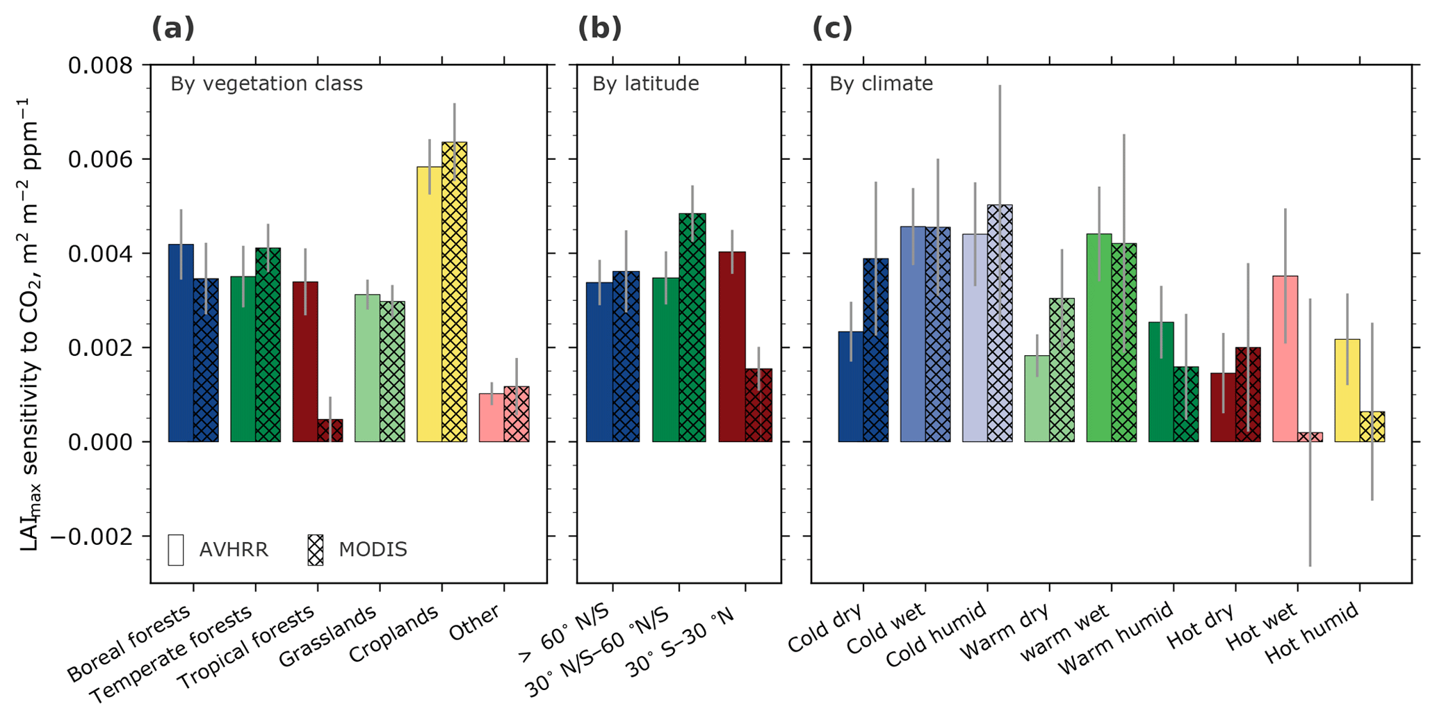
Figure 2 Bar charts showing regression slopes of LAI_max against atmospheric CO₂ concentration for broad vegetation classes (a) (Olson et al., 2001; Fritz et al., 2015), latitudinal bands (b), and climate regimes (c). The class “Other” includes deserts, mangroves, barren and urban land, snow and ice, and permanent wetlands. The climatic boundaries are defined as follows: cold: <10 ^∘C; warm: >10 and <25 ^∘C; hot: >25 ^∘C; dry: <500 mm a⁻¹; wet: >500 and <1000 mm a⁻¹; humid: >1000 mm a⁻¹. Sensitivities evaluated from data from two satellite-borne sensors are shown, AVHRR (1982–2016; Pinzon and Tucker, 2014) and MODIS (2000–2016; Yan et al., 2016a, b). Gray bars indicate the standard error of the best linear fit.

2.3 Earth system model simulations

We analyzed recent climate–carbon simulations of seven ESMs participating in the fifth phase of the Coupled Model Intercomparison Project, CMIP (Taylor et al., 2012). The model-simulated data were obtained from the Earth System Grid Federation, ESGF (https://esgf-data.dkrz.de/projects/esgf-dkrz/, last access: 21 September 2018). Seven ESMs provide output for the variables of interest (GPP, CO₂, LAI, and near-surface air temperature) for simulations titled esmHistorical, RCP4.5, RCP8.5, 1pctCO2, esmFixClim1, and esmFdbk1. It is the same set of models analyzed in Wenzel et al. (2016) and Winkler et al. (2019). The individual model setups and components are illustrated in more detail in various studies, such as Arora et al. (2013), Wenzel et al. (2014), Mahowald et al. (2016), and Winkler et al. (2019).

The esmHistorical simulation spanned the period 1850 to 2005 and was driven by observed conditions such as solar forcing, emissions or concentrations of short-lived species, natural and anthropogenic aerosols or their precursors, land use, and anthropogenic and volcanic influences on atmospheric composition. The models are forced by prescribed anthropogenic CO₂ emissions rather than atmospheric CO₂ concentrations.

Several Representative Concentration Pathways (RCPs) have been formulated describing different trajectories of greenhouse gas emissions, air pollutant production, and land use changes for the 21st century. These scenarios have been designed based on projections of human population growth, technological advancement, and societal responses (van Vuuren et al., 2011; Taylor et al., 2012). We analyzed simulations forced with specified concentrations of a high emissions scenario (RCP8.5) and a medium mitigation scenario (RCP4.5) reaching a radiative forcing level of 8.5 and 4.5 W m⁻² at the end of the century, respectively. These simulations were initialized with the final state at the end of the historical runs and spanned the period 2006 to 2100.

The 1pctCO2 simulation is an idealized fully coupled carbon–climate simulation initialized from a steady state of the preindustrial control run and atmospheric CO₂ concentration prescribed to increase 1 % yr⁻¹ until a quadrupling of the preindustrial level. The simulations esmFixClim and esmFdbk aim to disentangle the two carbon cycle feedbacks in response to rising CO₂ analogous to the 1pctCO2 setup. In esmFixClim CO₂-induced climate change is suppressed (i.e., the radiation transfer model has a constant preindustrial CO₂ level), while the carbon cycle responds to increasing CO₂ concentration (vice versa for esmFdbk; Taylor et al., 2012; Arora et al., 2013).

2.4 Estimation of greening sensitivities

We largely follow the methodology detailed in Winkler et al. (2019). For both model and observational data, the two-dimensional global fields of LAI and the driver variables are cropped according to different classification schemes (namely climatic regimes, latitudinal bands, and vegetation classes; Olson et al., 2001; Fritz et al., 2015). The aggregated values are area-weighted, averaged in space, and temporally reduced to annual estimates dependent on the variable: annual maximum LAI, annual average atmospheric CO₂ concentration, and growing degree days (GDD0, yearly accumulated temperature of days with near-surface air temperature > 0 ^∘C).

We use a standard linear regression model to derive the historical greening sensitivities in models and observations alike (for details see the Methods section entitled “Estimation of historical LAI_max sensitivity” in Winkler et al., 2019). On the global scale, LAI_max is assumed to be a linear function of atmospheric CO₂ concentration. For the temperature-limited high northern latitudes, we also have to account for warming and include temperature as an additional driver. We do this using GDD0. Through a principal component analysis (PCA) of CO₂ and GDD0 we avoid redundancy from colinearity between the two driver variables but retain their underlying time trend and interannual variability (for details see the Methods section entitled “Dimension reduction using principal component analysis” in Winkler et al., 2019). In particular, the PCA is performed on large-scale aggregated values as well as on a pixel level to investigate spatial variations. We only retain the first principal component (denoted ω), which explains a large fraction of the variance in models and observations (for more details see Table 1 in the Supplement in Winkler et al., 2019). Figure A1 depicts the temporal development of CO₂ and GDD0 as well as their principal component ω for observations. For the NHLs, LAI_max is then formulated as a linear function of the proxy driver time series ω (Winkler et al., 2019). The best-fit gradients and associated standard errors of the linear regression model represent the LAI_max sensitivities, or greening sensitivities, and their uncertainty estimates, respectively.

3 Results and discussion

There are two parts to the EC methodology (Fig. 1) – a statistically robust relationship between modeled matching pairs of predictor–predictand values and an observed value of the predictor. The predictors are from a representative historical period. The predictands are modeled changes in a variable of interest at another forcing state of the system (e.g., potential future). The projection of the observed predictor on the modeled relation yields a constrained value of the predictand. A causal basis has to buttress the predictor–predictand relationship or the EC method may be spurious. For example, a meaningful coupling between concurrent changes in GPP and LAI_max with an increasing atmospheric CO₂ concentration underpins our specific case study in the NHLs; i.e., some of the enhanced GPP due to the rising CO₂ concentration is invested in additional green leaves by plants (Myneni et al., 1997a; Forkel et al., 2016; Zhu et al., 2016; Mao et al., 2016; Winkler et al., 2019). Figure 1 of the Supplement in Winkler et al. (2019) illustrates the specifics of the causal link underlying this predictor–predictand relationship. This tight coupling ensures an approximately constant ratio of predictand to predictor across the models within the ensemble, thus setting up the potential for deriving an EC estimate. Uncertainty in the constrained estimate depends on the observed predictor and modeled relationship, aside from the goodness of fit of the latter (Fig. 1). These are detailed below.

3.1 Uncertainty in observed predictor due to data source

We investigate observational uncertainty using LAI data from two different sources, AVHRR (1∕12^∘) and MODIS (1∕20^∘), and spatially aggregating these over broad vegetation classes, latitudinal bands, and climatic regimes. The observed large-scale LAI_max sensitivities to CO₂ forcing are always positive (greening) irrespective of the source data and the method of aggregation (Fig. 2, Table 1). Overall, MODIS-based estimates have higher uncertainty because of the shorter length of the data record (17 years). The failure to reliably estimate sensitivities in tropical forests (also in the latitudinal band 30^∘ S–30^∘ N and in hot, wet, and humid climatic regimes; see Table 1 and Fig. 2) is due to the saturation of optical remote sensing data over dense vegetation (LAI_max>5) and problems associated with high aerosol content and ubiquitous cloudiness. In other regions, the estimated sensitivities are comparable across sensors and aggregation schemes, in particular in the high-latitudinal band (>60^∘ N–S; AVHRR: $(\mathrm{3.4}\pm \mathrm{0.5})\times {\mathrm{10}}^{-\mathrm{3}}$, MODIS: $(\mathrm{3.6}\pm \mathrm{0.9})\times {\mathrm{10}}^{-\mathrm{3}}$ m² m⁻² ppm⁻¹ CO₂). This aligns with previous studies reporting a net increase in green leaf area across the high latitudes during the observational period (Myneni et al., 1997b; Zhu et al., 2016; Forkel et al., 2016).

Table 1 Coefficients of determination (R²) of LAI_max sensitivity to CO₂ for different large-scale aggregated regions. Data are from two optical remote sensors of different time length, AVHRR (1982–2016) and MODIS (2000–2016). Asterisks denote nonsignificant values: ${}^{**}$ p>0.1; ^* p>0.05.

This analysis illustrates the applicability and limitations of using observed greening sensitivities to CO₂ forcing as a constraint on photosynthetic production. For example, data from both AVHRR and MODIS sensors provide a comparable estimate of greening sensitivity in the colder high latitudes (boreal forests and tundra vegetation classes; Winkler et al., 2019). In the lower latitudes, however, the discrepancies among the two sensors indicate a considerable observational uncertainty and thus no robust estimation of the observed predictor is possible.

3.2 Uncertainty due to spatial aggregation

We focus further analyses on the NHL region (>60^∘ N; Fig. 2b) for two reasons. First, the direct human impact (i.e., land management) can be neglected in the high latitudes, and thus we can assume that the observed changes reflect the response of natural ecosystems. Second, the observational evidence of increased plant productivity in recent decades is well established (e.g., Sect. 3.1; Keeling et al., 1996; Myneni et al., 1997a; Graven et al., 2013; Forkel et al., 2016; Wenzel et al., 2016) – an important requisite in defining a robust predictor.

In addition to the physiological effect of CO₂, warming also plays a key role in controlling plant productivity in NHL temperature-limited ecosystems and thus vegetation greenness. To avoid redundancy from colinearity between CO₂ and GDD0, we reduce dimensionality by performing a principal component analysis of the two driver variables (Sect. 2.4). The resulting first principal component explains most of the variance and retains the trend and year-to-year fluctuations in both CO₂ and GDD0. Therefore, we obtain a proxy driver (hereafter denoted ω) that represents the overall forcing signal causing observed vegetation greenness changes in NHLs (Fig. A1). Accordingly, greening sensitivity for the entire NHL area is derived as a response to ω, the combined forcing signal of rising CO₂ and warming. This procedure also enables better comparability between observations and models because varying strengths of the physiological and radiative effects of CO₂ among models are taken into account (Sect. 3.3–3.5).

The vegetated landscape in the NHL region is heterogeneous, with boreal forests in the south, vast tundra grasslands to the north, and shrublands in between. The species within each of these broad vegetation classes respond differently to changes in key environmental factors. Even within a species, such responses might vary due to different boundary conditions, such as topography, soil fertility, and micrometeorological conditions. How this fine-scale variation in greening sensitivity impacts the aggregated value is assessed below.

The distribution of greening sensitivities from all NHL pixels is slightly skewed towards the positive (blue histogram). The mean value of this distribution (blue dashed line) is comparable to the sensitivity estimate derived from the spatially averaged NHL time series (dashed yellow line; Fig. 3). Based on the Mann–Kendall test (p>0.1), over half of the pixels (54 %) show positive statistically significant trends (greening), while about 10 % show browning trends (possibly due to disturbances; Goetz et al., 2005). The distribution of these statistically significant sensitivities (red histogram) therefore has two modes, a weak browning and a dominant greening mode, resulting in a substantially higher mean value (red dashed line) in comparison to the spatially averaged estimate (dashed yellow line; Fig. 3). Thus, by taking into account the remaining 36 % of nonsignificantly changing pixels (as in the NHL spatially averaged estimate), an additional source of uncertainty is possibly introduced. The mean sensitivity value is, of course, higher when only pixels showing a greening trend are considered in the analysis (green dashed line; Fig. 3). These are the only areas in NHLs that actually show a large increase in plant productivity and consequently significant changes in leaf area.

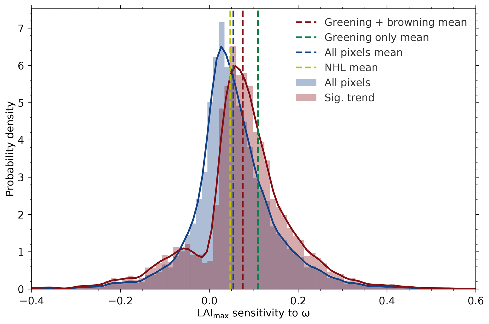
Figure 3 Histograms and associated probability density functions (Gaussian kernel density estimation) of observed LAI_max sensitivity to ω at pixel scale for the northern high-latitudinal band (>60^∘ N, data from AVHRR sensor). Blue depicts the distribution of LAI_max sensitivities of all pixels and red is for pixels with statistically significant (Mann–Kendall test, p<0.1) greening or browning trends (the dashed lines denote the respective mean value). The green dashed line shows the mean value of “greening” pixels only, whereas the dashed yellow line shows the LAI_max sensitivity to ω for the entire northern high-latitudinal belt.

The model output of several ESMs (CMIP5) reveal similar pixel-level variation in both the predictor (LAI_max to ω, historical simulation; Sect. 2.3) and associated changes in the predictand (GPP, 1pctCO2; Sect. 2.3), although ESMs operate on much coarser resolution (Fig. A2; see also Anav et al., 2013, 2015). Due to the coupling of the predictor and predictand, the distribution of pixels with significant changes is approximately the same for the two variables (Fig. A2). Accordingly, averaging the equally distributed estimates likely does not affect the predictor–predictand relationship in the model ensemble (Fig. 1). Consequently, if all spatial gridded data arrays are consistently processed to spatially aggregated estimates, each predictand and predictor (observed and modeled) estimate contains a coherent component of spatial variations. In other words, considering browning and nonsignificant pixels results in a lower overall LAI_max sensitivity in NHLs, which in turn leads to a lower constrained estimate of ΔGPP in NHLs. This is consistent with the underlying relationship between the predictor and predictand. On a related note, Bracegirdle and Stephenson (2012a) suggest that this source of error is not significantly dependent on the spatial resolution when comparing model subsets from high to low resolution.

The above analysis confirms that spatially averaged estimates are approximations containing a random error component due to the inclusion of data from insignificantly changing pixels and a systematic bias component from pixels of reversed sign. This uncertainty is relevant to the EC method, wherein the observed sensitivity decisively determines the constrained estimate from the ensemble of ESM projections (Kwiatkowski et al., 2017; Winkler et al., 2019). However, if spatial variations are treated consistently as an inherent component of observations and models, the EC method is only slightly susceptible to this source of uncertainty.

3.3 Uncertainty due to temporal variations

We rely on long-term CMIP5 ESM simulations covering the historical period 1850 to 2005 (Sect. 2.3) to assess the temporal variation in the predictor variable because of the shortness of the observational record. Three representative models (CESM1-BGC, MIROC-ESM, and HadGEM2-ES) spanning the full range of NHL greening sensitivities in the CMIP5 ensemble (Winkler et al., 2019) are selected for this analysis. For each model, LAI_max sensitivity to ω in moving windows of different lengths is evaluated (15, 30, and 45 years; Figs. 4 and A3). The analysis reveals two crucial aspects that highlight how temporal variations impair the comparability of the predictor variable between models and observations – an essential component of the EC approach.

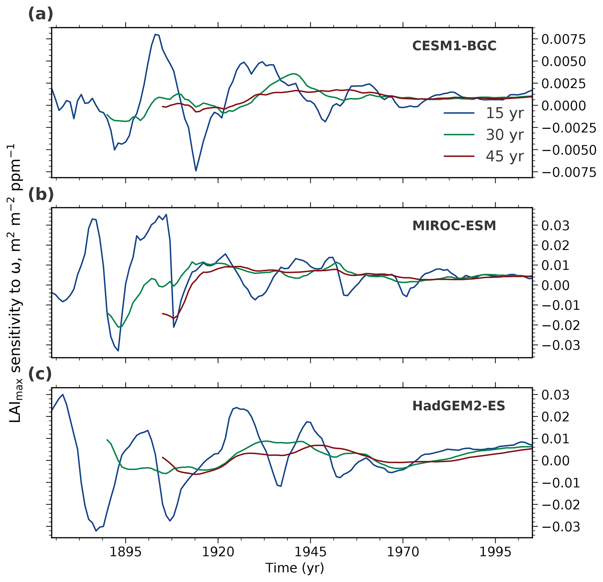
Figure 4 Temporal variation of LAI_max sensitivity to ω in three selected CMIP5 models spanning the full range from low-end (CESM1-BGC, a), to closest to observations (MIROC-ESM, b), to high-end (HadGEM2-ES, c). The colored lines show LAI_max sensitivity variations for moving windows of varying length: 15 (blue), 30 (green), and 45 (red) years over the historical period from 1860 to 2005.

First, the window locations of modeled and observed predictor variables have to match. If the forcing in the simulations is low, for example in the second half of the 19th century when the CO₂ concentration was increasing slowly, interannual variability dominates and LAI_max sensitivity cannot be accurately estimated irrespective of the window length (Figs. 4 and A3). With increasing forcing over time (rising yearly rate of CO₂ emissions and, consequently, the concentration), the signal-to-noise ratio increases and LAI_max sensitivity to ω estimation stabilizes, for example in the second half of the 20th century. Therefore, LAI_max sensitivities estimated at different temporal locations result in noncomparable values and eventually a false constrained estimate (details in Sect. 3.4). As an example, modeled sensitivities based on a 30-year window centered on the year 1900, when the CO₂ level increased by 10 ppm, and observed sensitivity estimated from a 30-year window centered on the year 2000, when the CO₂ level increased by 55 ppm, describe different states of the system and therefore should not be contrasted in the EC method.

Second, in addition to the temporal location, window lengths also have to match between observations and models. For all three models, sensitivities estimated from 15-year chunks show high variability, and thus a 15-year record is perhaps too short to obtain robust estimates. The LAI_max sensitivity estimation becomes more stable with strengthening forcing and increasing window length (Figs. 4 and A3). As a consequence, using short-term observed sensitivity as a constraint on long-term model projections results in an incorrect EC estimate. Hence, the MODIS sensor record is, on the one hand, too short and does not, on the other hand, overlap temporally with the historical CMIP5 forcing. Therefore, it does not provide a robust predictor in this EC study.

3.4 Level and time rate of CO₂ forcing

The EC method raises an obvious question – does it not implicitly assume that the key operative mechanisms underpinning the EC relation remain unchanged because a future system state is being predicted based on its past behavior? To be specific, we are attempting to predict GPP at a future point in time based on greening sensitivity inferred from the past. Does this not require the assumption that the key underlying relationship that makes this prediction possible, namely a robust coupling between contemporaneous changes in GPP and LAI_max, remains unchanged from the past to the future? To address this question, we resort to the CMIP5 idealized simulation (1pctCO2), wherein atmospheric CO₂ concentration increases 1 % annually, starting from a preindustrial level of 284 ppm until a quadruple of this value is reached (Sect. 2.3). We limit the analysis to the three models (CESM1-BGC, MIROC-ESM, and HadGEM2-ES) that bracket the full range of GPP enhancement and LAI_max sensitivity in the original seven-ESM ensemble (Winkler et al., 2019).

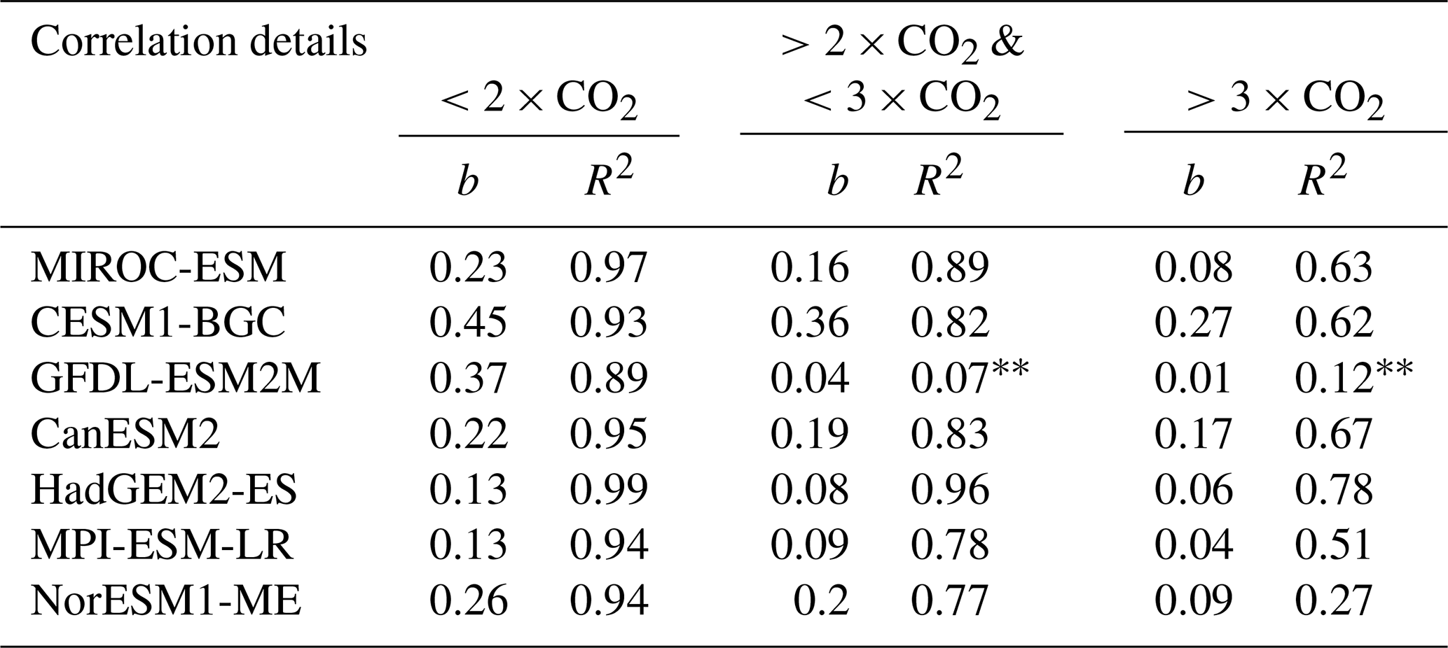
The relationship between simultaneous changes in GPP and LAI_max remains linear for all CMIP5 models in the range 1×CO₂ to 2×CO₂ (Figs. 5 and A4, Table 2). With concentration increasing beyond 2×CO₂, all models show a weakening correlation (R²; Table 2) and decreasing slope (b; Table 2) of this relationship (Figs. 5 and A4), suggesting a saturating rate of allocation of additional GPP to new leaves at higher levels of CO₂. Consequently, LAI_max sensitivity to increasing CO₂ and associated warming decreases. At and over 4×CO₂ (1140 ppm), a level unlikely to be seen in the near future, there appears to be no relationship between ΔGPP and ΔLAI_max in some models. This raises the question of to what extent the weakening of the relationship between the predictor and predictand in each model at higher CO₂ concentrations affects the EC analysis (Fig. 1). To shed light on this matter, we perform the following thought experiment.

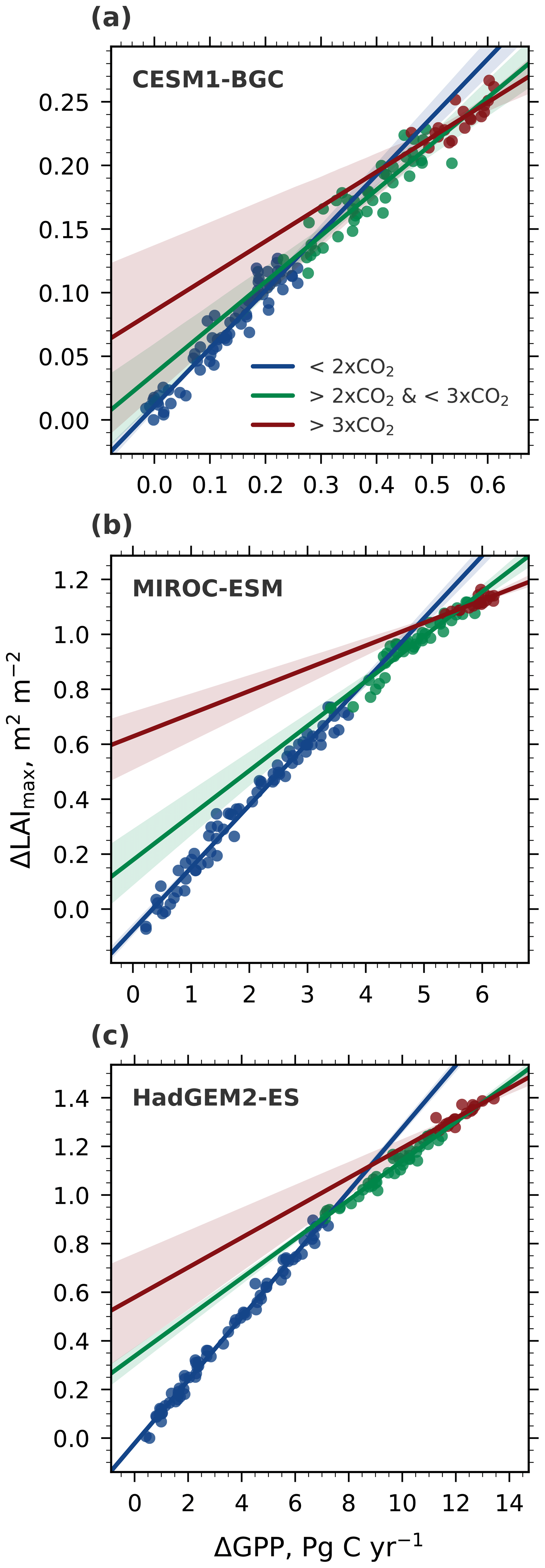
Figure 5 Correlation of ΔLAI_max and ΔGPP with increasing CO₂ forcing, starting from a preindustrial concentration of 280 ppm (1×CO₂) to 4×CO₂ (CMIP5 1pctCO2 simulations). Results are shown for three selected CMIP5 models spanning the full range of LAI_max sensitivity to ω: low-end: CESM1-BGC (a), closest to observations: MIROC-ESM (b), and high-end: HadGEM2-ES (c). Blue colored dots show the relation between 1×CO₂ and 2×CO₂, green colored dots between 2×CO₂ and 3×CO₂, and red colored dots between 3×CO₂ and 4×CO₂. The respective colored lines represent the best linear fit through those dots and the shading represents the 95 % confidence interval.

Table 2 Slopes (b) and coefficients of determination (R²) for regression between changes in LAI_max against changes in annual mean GPP for the NHLs at different atmospheric CO₂ levels in all available CMIP5 models (1pctCO2 simulation). Asterisks denote nonsignificant values: ${}^{**}$ p>0.1; ^* p>0.05.

Understanding the relationship and interplay between forcing (increasing CO₂ concentration), the predictor (LAI_max sensitivity), and the predictand (ΔGPP) is key to evaluating the EC method. We conceive four possible scenarios of how the system might behave with increasing forcing. For simplicity, we assume a linearly increasing CO₂ concentration; LAI represents LAI_max, and GPP refers to its annual value below (Fig. 6). The four scenarios are as follows: all linear, all nonlinear (saturation), and two mixed linear–nonlinear cases (Table A1). We emulate a multi-model ensemble by applying different random parameterizations for the linear and saturation (the hyperbolic tangent function) responses of GPP to CO₂ and of LAI to GPP. One of these realizations is assumed to represent pseudo observations (dashed lines, Fig. 6). We discuss one case in detail for illustrative purposes (no. 3; Table A1).

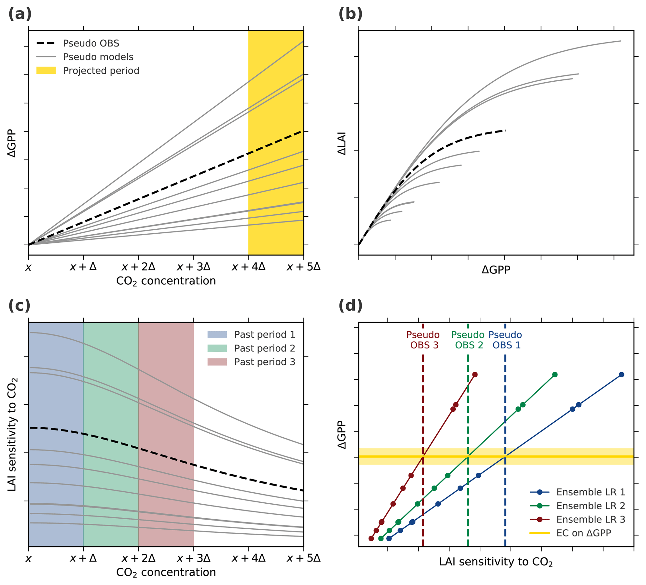
Figure 6 Thought experiment to examine the applicability of EC analysis under the assumption of an idealized linear–nonlinear behavior of the system (Case 3, Table A1). (a) Changes in GPP relate linearly to changes in CO₂ concentration. The yellow band marks the projection period of interest, i.e., the period of CO₂ concentration from x+4Δ to x+5Δ. (b) The increment in LAI with increasing GPP is assumed to decrease with rising CO₂ concentration (described by a hyperbolic tangent function). The parameterization in the linear and nonlinear functions for pseudo observations (dashed black line) as well as models (solid gray lines) is determined randomly for each model. (c) The diagnostic variable, LAI sensitivity to CO₂, decreases with increasing CO₂ as a consequence of the nonlinear relation between ΔGPP and ΔLAI. The colored bands indicate three “past” periods from x to x+Δ (blue), x+Δ to x+2Δ (green), and x+2Δ to x+3Δ (red). (d) Linear relationships among the pseudo model ensembles (Ensemble LR, colored lines) between LAI sensitivities to CO₂ of the three past periods and ΔGPP from the projected period. Colored dots mark different models and the dashed lines represent associated pseudo observations for the respective historical period. The solid yellow line depicts the constant EC on projected ΔGPP irrespective of the past period.

In scenario 3, ΔGPP increases linearly with increasing CO₂ (Fig. 6a), while ΔLAI ∕ ΔGPP saturates (Fig. 6b). The LAI sensitivity to CO₂ weakens with increasing forcing (Fig. 6c) as a response to the saturation of GPP allocation to leaf area. We derive LAI sensitivities to CO₂ for three different periods (“past periods” in Fig. 6c) to constrain ΔGPP at a much higher CO₂ level (“projected period” in Fig. 6a). Next, we apply the EC method on these pseudo projections of ΔGPP, relying on LAI sensitivities derived from the three past periods (Fig. 6d). The EC method is applicable even at a low forcing level (past period 1) in this simplified scenario because we neglect the stochastic internal variability of the system. The slope of the emergent linear relationship increases (Fig. 6d) as modeled LAI sensitivities decrease with a rising CO₂ concentration (Fig. 6c). The observational constraint on future ΔGPP, however, remains nearly the same because pseudo-observed LAI sensitivity also weakens at higher CO₂ levels (dashed lines, Fig. 6c and d). Thus, the three EC estimates of ΔGPP are approximately identical (Fig. 6d) and independent of the forcing level during past periods. With intensified forcing, the relationship between the predictor and predictand remains linear within the model ensemble, although their relationship becomes nonlinear within each model and, crucially, in reality as well. In other words, as long as the models agree on the occurrence and strength of saturation for given forcing, i.e., the dynamics of the system, the inter-model variations of the predictor and predictand relate linearly within the ensemble (Fig. 6). The same behavior is also seen in the other three scenarios (Table A1; Figs. A5 and A6).

Nevertheless, with ever increasing forcing and associated steepening of the emergent linear relationship, the LAI sensitivity loses its explanatory power at some point because the linear relationship eventually lies within the observational uncertainty and no meaningful constraint can be derived. This and disagreement between models on system dynamics are ultimate limits of the EC method. Interestingly, we find that all CMIP5 models agree on the occurrence of saturation but slightly disagree on the strength of saturation for given CO₂ forcing (Figs. 5 and A4, and Table 2). Further, we find that the “all nonlinear” scenario best describes the dynamics of the system in the forcing range from 1×CO₂ to 4×CO₂. However, the saturation of LAI to GPP happens at a lower CO₂ level than saturation of GPP to CO₂. Still, inferences from the interpretation of Case 3 (Fig. 6) are equally applicable.

Results from the above thought experiment also highlight the importance of matching window locations and lengths between models and observations, as discussed earlier (Sect. 3.3). For instance, taking LAI sensitivity from past period 2 (green dashed line, Fig. 6d) as an observational constraint on the multi-model linear relationship based on past period 3 (red solid line, Fig. 6d) results in a significant overestimation of constrained ΔGPP (intersection of the two lines, Fig. 6d).

The above analysis confirms that the constrained GPP estimate at one future period (e.g., 2×CO₂) is nearly independent of the past periods from which the observational sensitivities are derived. Now, we evaluate the EC method wherein the sensitivity from one past period is used to obtain constrained GPP estimates at different periods in a potential future, i.e., progressively farther down the timeline of a CO₂-enriched world. We utilize the greening sensitivity derived from 35 years of observed LAI_max data (AVHRR; Sect. 2.1) and apply the EC method to CMIP5 1pctCO2 simulations. The sensitivities in this case are due to forcing from both the CO₂ increase and associated warming during the observational period (Sect. 2.4). We seek constrained GPP estimates for the NHLs at different CO₂ levels (2×CO₂, 3×CO₂, and 4×CO₂).

Winkler et al. (2019) previously reported a strong linear relationship between modeled contemporaneous changes in LAI_max and GPP arising from the combined radiative and physiological effects of CO₂ enrichment until 2×CO₂ in the CMIP5 ensemble. As a result, models with low LAI_max sensitivity to ω project lower ΔGPP for a given increment of CO₂ concentration and vice versa. Thus, the large variation in modeled historical LAI_max sensitivities linearly maps to the variation in ΔGPP at 2×CO₂ (blue line, Fig. 7a; Winkler et al., 2019). At higher levels, such as 3×CO₂ (green line, R²=0.93) and 4×CO₂ (red line, R²=0.88), this linear relationship within the model ensemble, while still present, weakens (Fig. 7a; Table 3). This is because the CMIP5 models do not agree on the strength of the saturation effect at higher CO₂ levels (Figs. 5 and A4). The increment in constrained GPP estimates for successive equal increments of CO₂ decreases due to the saturation effect in all CMIP5 models (dashed horizontal lines, Fig. 7a). For example, the change in GPP between 3×CO₂ and 4×CO₂ (ΔGPP ∼ 1.06 Pg C yr⁻¹; Table 3) is much lower than between 2×CO₂ and 3×CO₂ (ΔGPP ∼ 2.34 Pg C yr⁻¹; Table 3).

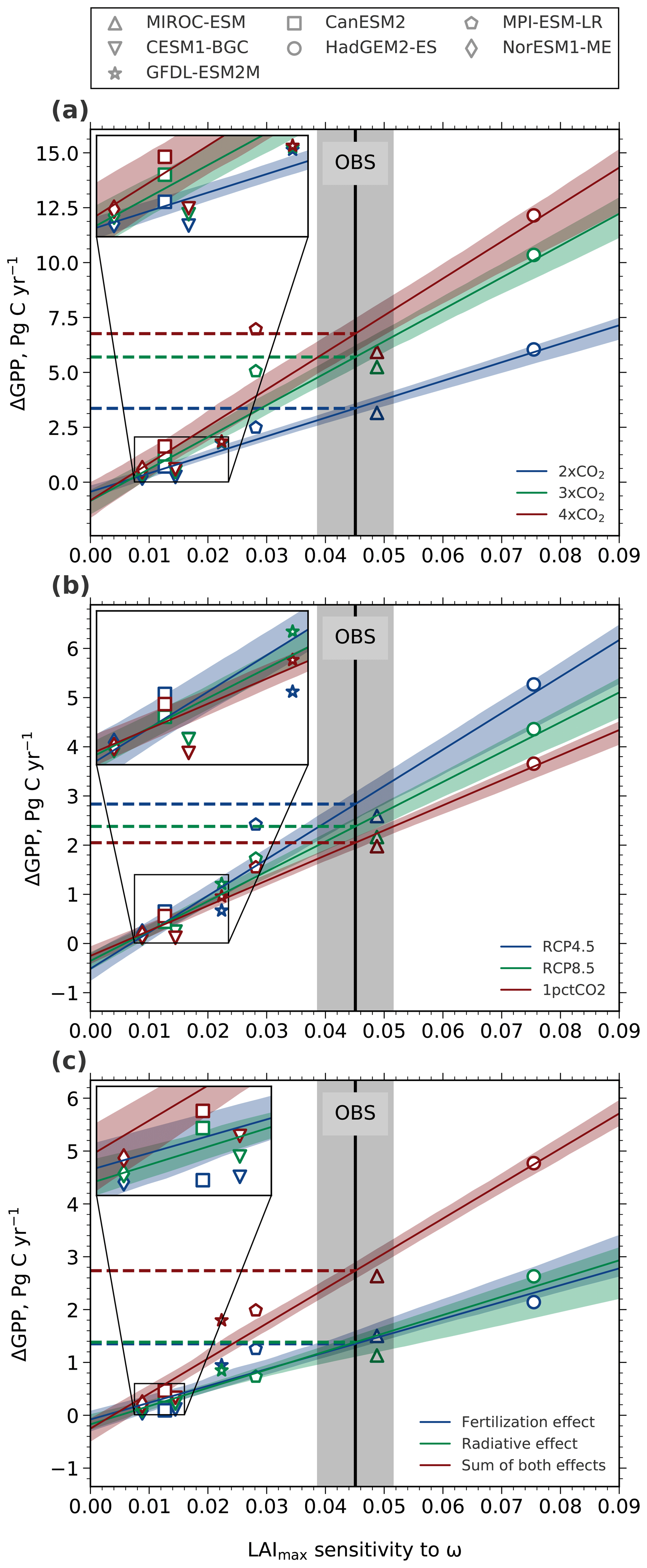
Figure 7 Linear relationships between the historical sensitivity of LAI_max to ω and an absolute increase in GPP at different levels (a), different time rates (b), and the effects of rising CO₂ (c). The solid black line depicts the observational sensitivity including the standard error (gray shading). Each CMIP5 model is represented by a distinct marker (legend at the top). The colored lines show the best linear fits including the 68 % confidence interval estimated by bootstrapping across the model ensemble. The colored dashed lines indicate the derived constraints on ΔGPP. (a) Absolute changes in GPP at different levels of CO₂: 2×CO₂ (blue), 3×CO₂ (green), and 4×CO₂ (red). (b) Absolute changes in GPP for a rising CO₂ concentration from 380 to 535 ppm at different time rates: RCP4.5 (90-year, blue), RCP8.5 (45-year, green), and 1pctCO2 (30-year, red). (c) Absolute changes in GPP due to the two disentangled effects of CO₂ at 2×CO₂ in idealized simulations: fertilization effect (esmFixClim1, blue), radiative effect (esmFdbk1, green), and the sum of both effects (red).

Table 3 Coefficients of determination (R²) of the emergent linear relationships in Fig. 7 (asterisks denote nonsignificant values: ${}^{**}$ p>0.1; ^* p>0.05). ECs on ΔGPP (upper and lower bound of uncertainty in square brackets) for different atmospheric CO₂ levels and fully coupled as well as idealized setups. The rightmost column shows the increase in ΔGPP for an increment of 1×CO₂. The lowermost section compares EC estimates of ΔGPP for equivalent changes in CO₂ concentration (CO₂ rises from 380 to 535 ppm) but for different time rates.

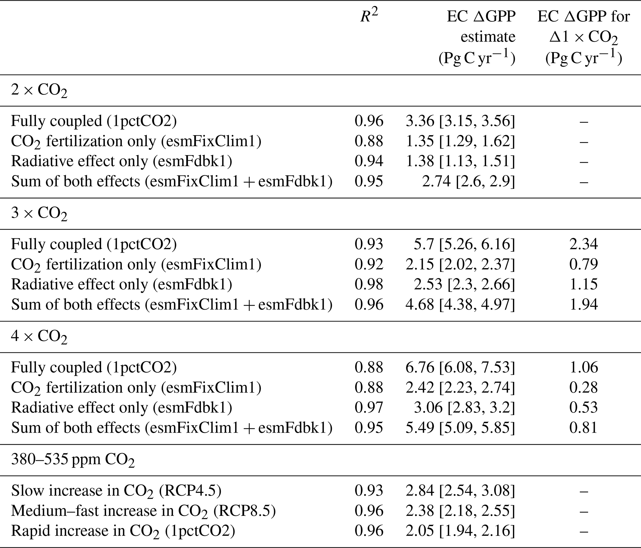
We have thus far focused on the magnitude of CO₂ concentration change and not on the time rate of this change. For example, a given amount of change in CO₂ concentration, say 200 ppm, can be realized over different time periods, say over 100 or 150 years. The problem of varying rates of CO₂ concentration change is implicitly encountered when ESMs are executed under different forcing scenarios, such as RCPs (Sect. 2.3). A question then arises as to whether the constrained predictand estimate is independent of the time rate of CO₂ concentration change and dependent only on the magnitude of CO₂ concentration change. To investigate this aspect of forcing, we extract GPP estimates at the same CO₂ concentration (535 ppm; final concentration in RCP4.5) from three simulations of different forcing rates and calculate the difference relative to a common initial CO₂ concentration (380 ppm; initial concentration of RCP scenarios). Hence, the magnitude of the forcing is the same but applied over different durations (RCP4.5: ∼90 years, RCP8.5: ∼45 years, and 1pctCO2: ∼30 years). A clear majority of the CMIP5 models show substantial differences in ΔGPP between the different pathways of CO₂ forcing. In general, GPP changes are higher for lower time rates of CO₂ forcing, i.e., forcing over longer time periods. As a consequence, the EC estimates of ΔGPP for the same increase in CO₂ concentration are scenario dependent (Fig. 7b; Table 3) – a counterintuitive result. For instance, in the RCP4.5 scenario (which is characterized by a lower rate of CO₂ increase) an increment of 155 ppm CO₂ yields a GPP enhancement of ∼2.84 Pg C yr⁻¹ (see Table 3). This GPP enhancement is ∼39 % and ∼20 % larger than in the 1pctCO2 run (∼2.05 Pg C yr⁻¹; Table 3) and the RCP8.5 (∼2.38 Pg C yr⁻¹; Table 3) scenario, respectively, for the same total increase in CO₂ concentration. Both these scenarios are characterized by a faster rate of CO₂ increase than RCP4.5. This analysis suggests that the vegetation response to rising CO₂ is pathway dependent, at least in the NHLs. One of the reasons for this could be species compositional changes in scenarios of low forcing rates, i.e., over longer time frames. This novel result, however, requires a separate in-depth study.

3.5 Effects of CO₂ forcing

A higher concentration of CO₂ in the atmosphere stimulates plant productivity through fertilization and radiative effects (Nemani et al., 2003; Leakey et al., 2009; Arora et al., 2011; Goll et al., 2017). The two effects can be disentangled in the model world by conducting simulations in a “CO₂ fertilization effect only” (esmFixClim1) and a “radiative effect only” (esmFdbk1) setup (Sect. 2.3). These are termed below as idealized model simulations. We investigate here whether historical runs and observations, which include both effects, can be used to constrain GPP changes in idealized CMIP5 simulations (as in Wenzel et al., 2016).

We find strong linear relationships between historical LAI_max sensitivity and ΔGPP for 2×CO₂ in both idealized setups (esmFixClim1: R²=0.92, esmFdbk1: R²=0.98; Table 3, Fig. 7c). Consequently, this linear relationship is also pronounced for calculated sums of both effects for each model (esmFixClim1 + esmFdbk1: R²=0.95; Table 3, Fig. 7c). This suggests that the two effects act additively on plant productivity, and thus each effect can be simply expressed in terms of a scaling factor of the total GPP enhancement. Hence, the application of the EC method on idealized simulations using real-world observations is conceptually feasible.

Interestingly, the two effects contribute about the same to the general increase in GPP at 2×CO₂ (esmFixClim1: ΔGPP ∼ 1.35 Pg C yr⁻¹, esmFdbk1: ΔGPP ∼ 1.38 Pg C yr⁻¹; Table 3, Fig. 7c). At higher concentrations, such as 3×CO₂ and 4×CO₂, the enhancement in GPP saturates in both idealized setups. However, the radiative effect becomes dominant relative to the CO₂ fertilization effect when CO₂ concentration exceeds 2×CO₂ (e.g., at 4×CO₂ esmFixClim1: ΔGPP ∼ 2.42 Pg C yr⁻¹, esmFdbk1: ΔGPP ∼ 3.06 Pg C yr⁻¹; Table 3). Therefore, we can expect that at some point in the future, NHL photosynthetic carbon fixation will benefit more from climate change (e.g., warming) than from the fertilizing effect of CO₂.

3.6 Uncertainties in the multi-model ensemble

Besides the methodological sources of uncertainty discussed above, the estimate of an EC may also be deficient due to inaccurate assumptions about the model ensemble. First, possible common systematic errors in a multi-model ensemble (i.e., the entire ensemble misses an unknown process that plays a key role in a high CO₂ world) are implicitly omitted in the EC approach; however, they could cause a general overestimation or underestimation of the constrained value (Bracegirdle and Stephenson, 2012b; Stephenson et al., 2012). Second, the set of forcing variables for historical simulations may be incomplete (i.e., not yet identified drivers of observed changes), and thus the comparability of observations and model simulations is limited (Flato et al., 2013). Third, the EC method can be overly sensitive to individual models of the ensemble, which has a bearing on the robustness of the constrained value (Bracegirdle and Stephenson, 2012b). Bracegirdle and Stephenson (2012b) proposed a diagnostic metric (Cook's distance) to test an ensemble for influential models. Fourth, the predictand–predictor relationship not only has to rely on a physical but also on a logical connection within the model ensemble. For instance, Wenzel et al. (2016) established a linear relationship between relative changes in the predictand taking the initial state into account (changes in GPP for a doubling of CO₂ relative to the initial preindustrial state) and a predictor neglecting the initial state (historical sensitivity of CO₂ amplitude to rising CO₂). This statistical relationship can be spurious because the model skills in simulating an accurate initial state and a plausible sensitivity to a forcing are not connected. These issues are to be contemplated when establishing an EC estimate and evaluating its robustness.

4 Conclusions

An in-depth analysis of the EC method is illustrated in this article through its application to projections of change in NHL photosynthesis under conditions of a rising atmospheric CO₂ concentration. Key conclusions highlighting the functionality of the EC method are presented below.

The importance of how the observational predictor is obtained cannot be emphasized enough because the EC method is particularly sensitive to observational uncertainty. The single observational estimate essentially determines the EC, whereas the emergent linear relationship is established based on a collection of multi-model estimates (each model gets “one vote”; however, some models might be more influential than others; Bracegirdle and Stephenson, 2012b). Hence, the observational uncertainty has a much larger bearing on the EC than the uncertainty of each individual model. To overcome this source of uncertainty, various meaningful observations should be taken into consideration when establishing the observed predictor.

Spatially aggregating observations and model output at different resolutions in the EC method constitutes another source of uncertainty. Predictors and predictands expressed as regional estimates (e.g., area-weighted mean of the NHLs) are approximations of complex fine-scale processes. Aggregation will inevitably introduce a random error component due to the inclusion of estimates from areas where the predictor does not change or a systematic bias from areas where the predictor has a reversed sign. Thus, the spatially aggregated variables are meaningful only if most of the region is in agreement about the response to CO₂ forcing (e.g., more than half of the NHLs is greening with rising CO₂). However, we find that the source of uncertainty related to spatial aggregation is of minor importance as long as spatial variations in observations and model simulations are treated consistently.

A large source of uncertainty is associated with the temporal variability of the predictor variable when comparing models and observations. Establishing a robust predictor requires evaluating temporal window lengths of sufficient duration (approximately 30 years) and their locations along the forcing timeline. Both window length and location should match between models and observations in the EC method. For example, the analysis in Wenzel et al. (2016) might have yielded different results and conclusions if the model and observational predictor sensitivities were temporally matched. We find that the relevance of window length decreases with increasing and accelerating forcing, depending on the magnitude of the natural and/or internal variability (signal-to-noise ratio) of the predictor variable.

The level, effect, and time rate of applied CO₂ forcing can have a bearing on the linear relationship between the predictand and predictor variables (Fig. 1). In our case study, the relationship underpinning the EC method, namely that between concurrent ΔGPP and ΔLAI_max, changes nonlinearly with an increasing forcing level (i.e., saturation with rising CO₂ concentration). The EC method can still be applied because the CMIP5 models agree on the nonlinear behavior of the system. However, at very high CO₂ concentrations the models diverge and this relation breaks down, at which point the EC method fails. The two dominant effects of a rising CO₂ concentration on vegetation, namely fertilization and radiative effects, appear to be approximately additive in terms of GPP enhancement to CO₂ forcing in the NHLs. Therefore, the EC method can be applied to constrain estimates of GPP due to one, the other, or both of the effects. The models, however, document a higher radiative effect than fertilization at concentrations exceeding 2×CO₂. Another intriguing conclusion from our analysis is that the time rate of forcing has an effect on GPP changes; that is, the projected GPP enhancement to CO₂ forcing seems to be dependent on how the forcing is applied over time, as in different scenarios or RCPs. This aspect is presently not well understood and requires further study.

The EC framework is widely promoted as observation-based evaluation tool for climate projections, especially in the context of the nascent CMIP6 ensemble (Eyring et al., 2019; Hall et al., 2019). Previous EC studies, however, exclusively focused on predictor–predictand combinations that exhibit so-called existent ECs (Hall et al., 2019); i.e., the predictor and predictand are found to relate linearly across the ensemble. In the context of ESM evaluation, nonexistent ECs, for which the predictor and predictand are found to be unrelated in the ensemble, are equally important. Since predictor and predictand variables are premised on our mechanistic process understanding, nonexistent ECs reveal a fundamental disagreement on the system dynamics among the models. This study encourages researchers to scrutinize these system dynamics in the predictor–predictand space and also report such nonexistent, yet expected, ECs in order to advance model development and evaluation.

Across different disciplines each EC and its set of predictors and predictands are unique to some extent and require an individual detailed examination. In this article, we addressed general potential sources of uncertainty and limitations in the EC method by means of a case study in carbon cycle research. Thus, the illustrated results are qualitatively transmissible to other sets of predictors and predictands and are generally relevant in Earth system sciences.

Appendix A

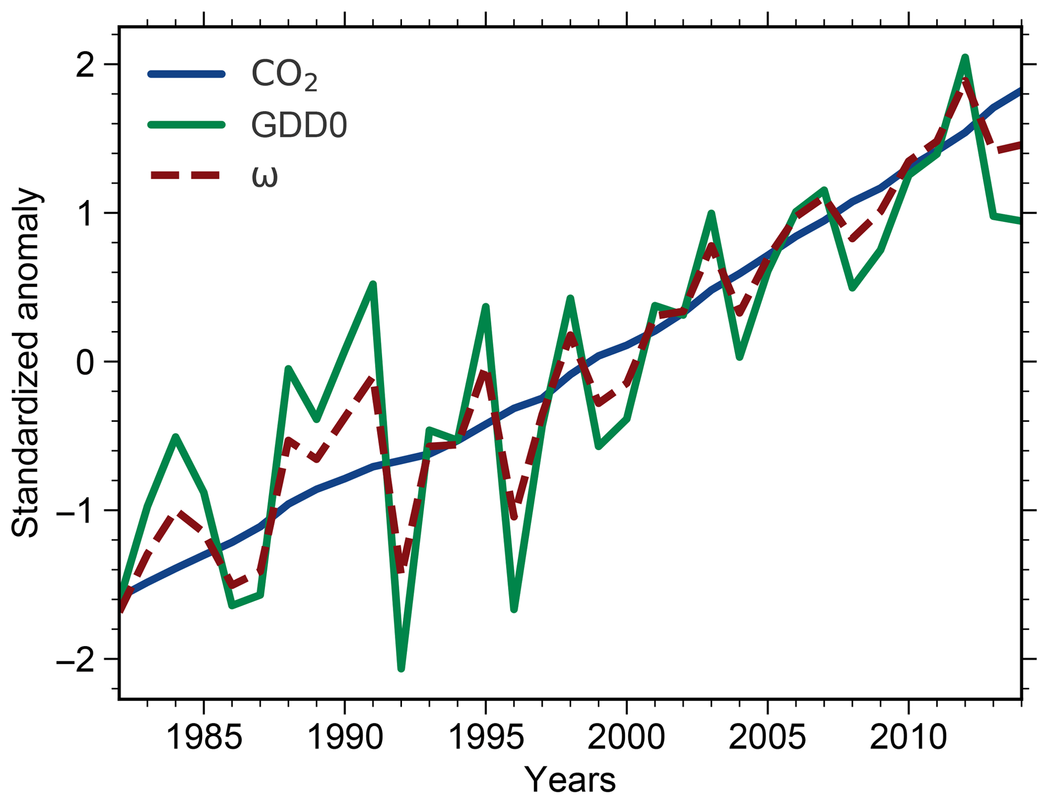
Figure A1 Standardized temporal anomalies of annual averaged atmospheric CO₂ concentration (blue solid line), area-weighted averaged GDD0 for NHLs (green solid line), and their leading principal component ω (red dashed line) in observations.

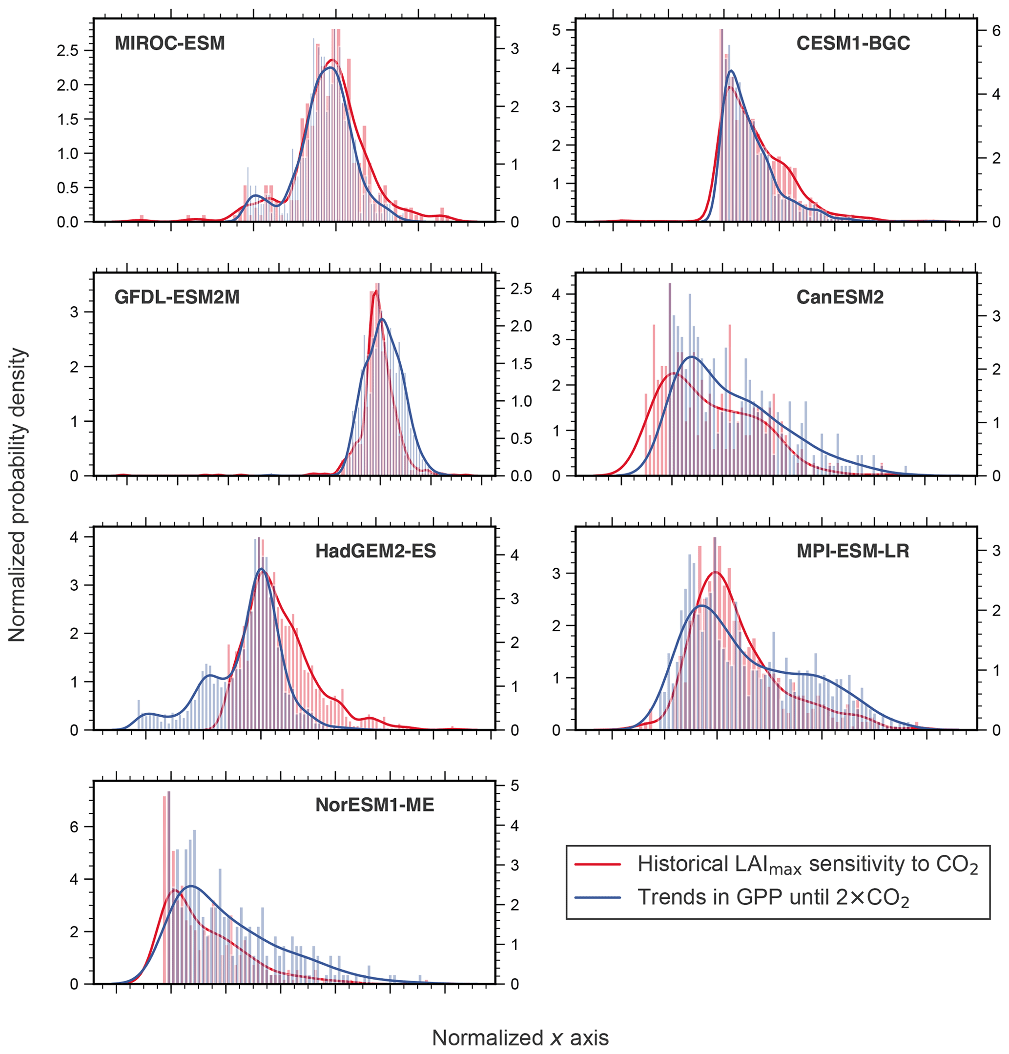
Figure A2 Similar pixel distribution of the predictor and predictand in each model, except HadGEM2-ES. Histograms and associated probability density functions (Gaussian kernel density estimation) of LAI sensitivity to ω (red, left y axis, historical simulations) and temporal trends in GPP (blue, right y axis, 1pctCO2, until 2×CO₂) for NHLs are shown for all CMIP5 models. Only significant pixels are included (Mann–Kendall test, p<0.1). To obtain comparability between the distributions, the x axis was normalized and has only a qualitative meaning.

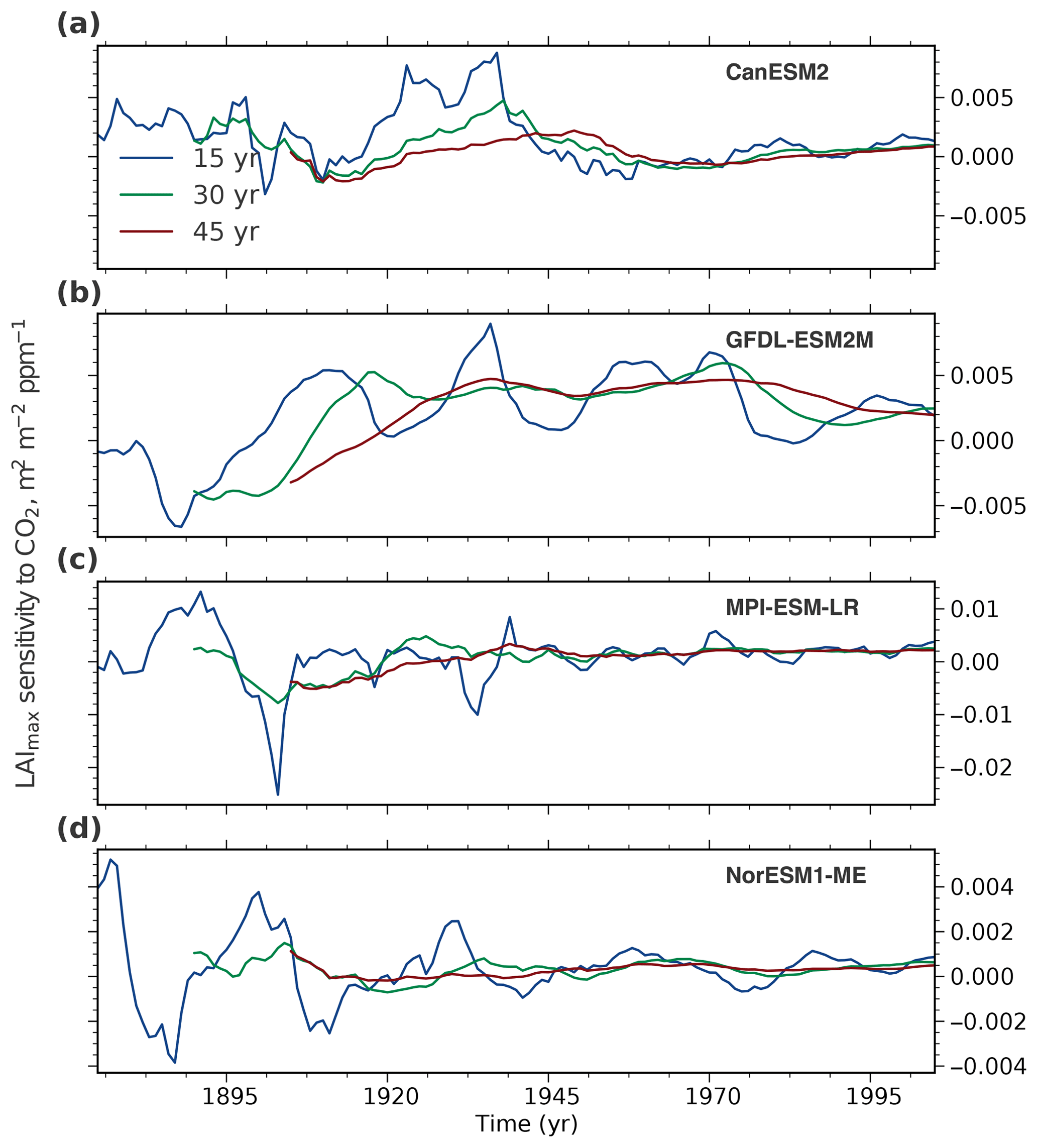
Figure A3 Temporal variation of LAI_max sensitivity to ω in four CMIP5 models analogous to Fig. 4. The colored lines show LAI_max sensitivity variations for moving windows of varying length: 15 (blue), 30 (green), and 45 (red) years over the historical period from 1860 to 2005.

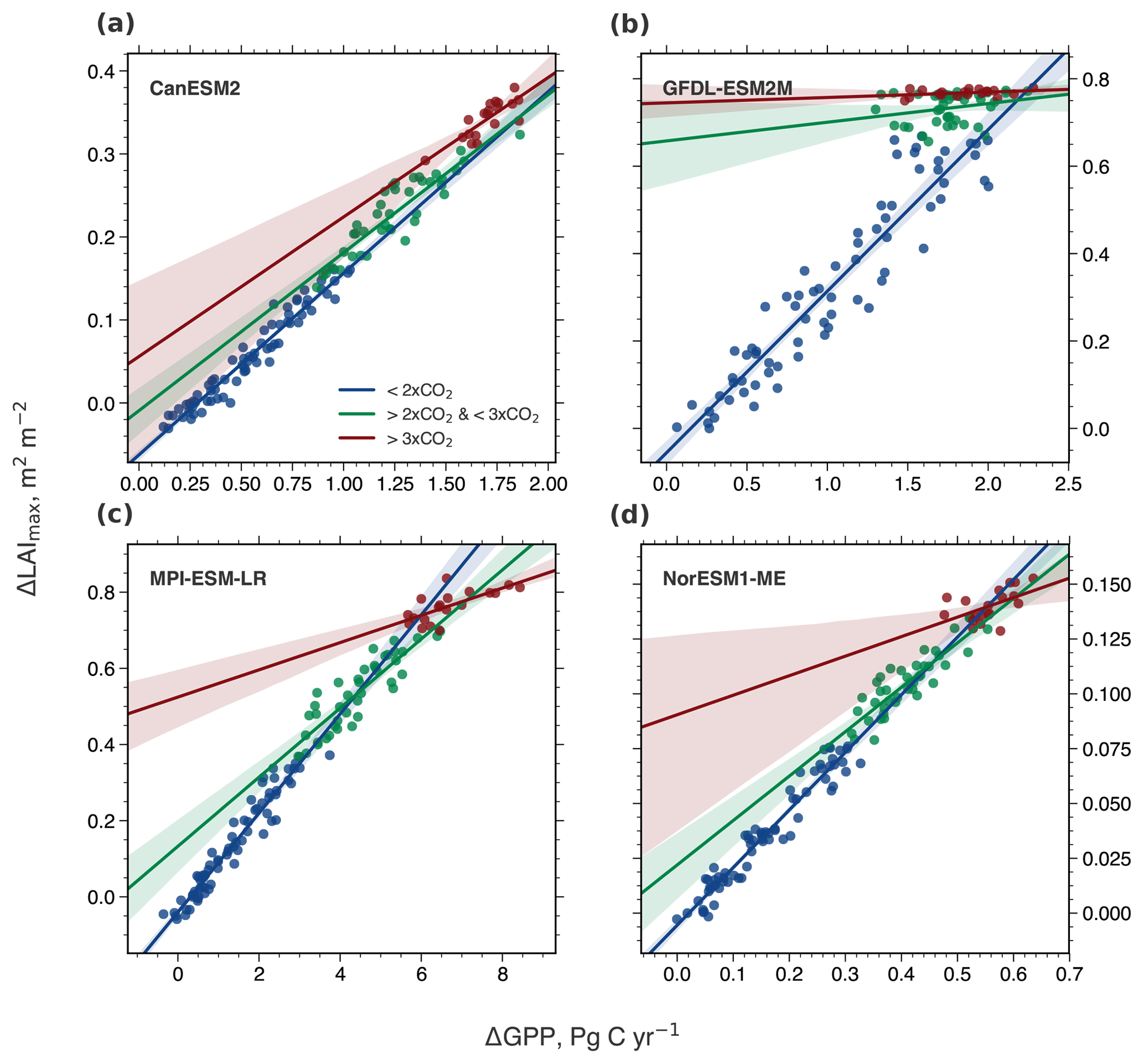
Figure A4 Correlation of ΔLAI_max and ΔGPP with increasing CO₂ forcing, starting from a preindustrial concentration of 280 ppm (1×CO₂) to 4×CO₂ (CMIP5 1pctCO2 simulations). Results are shown for four CMIP5 models analogous to Fig. 5. Blue colored dots show the relation between 1×CO₂ and 2×CO₂, green colored dots between 2×CO₂ and 3×CO₂, and red colored dots between 3×CO₂ and 4×CO₂. The respective colored lines represent the best linear fit through those dots and the shading represents the 95 % confidence interval.

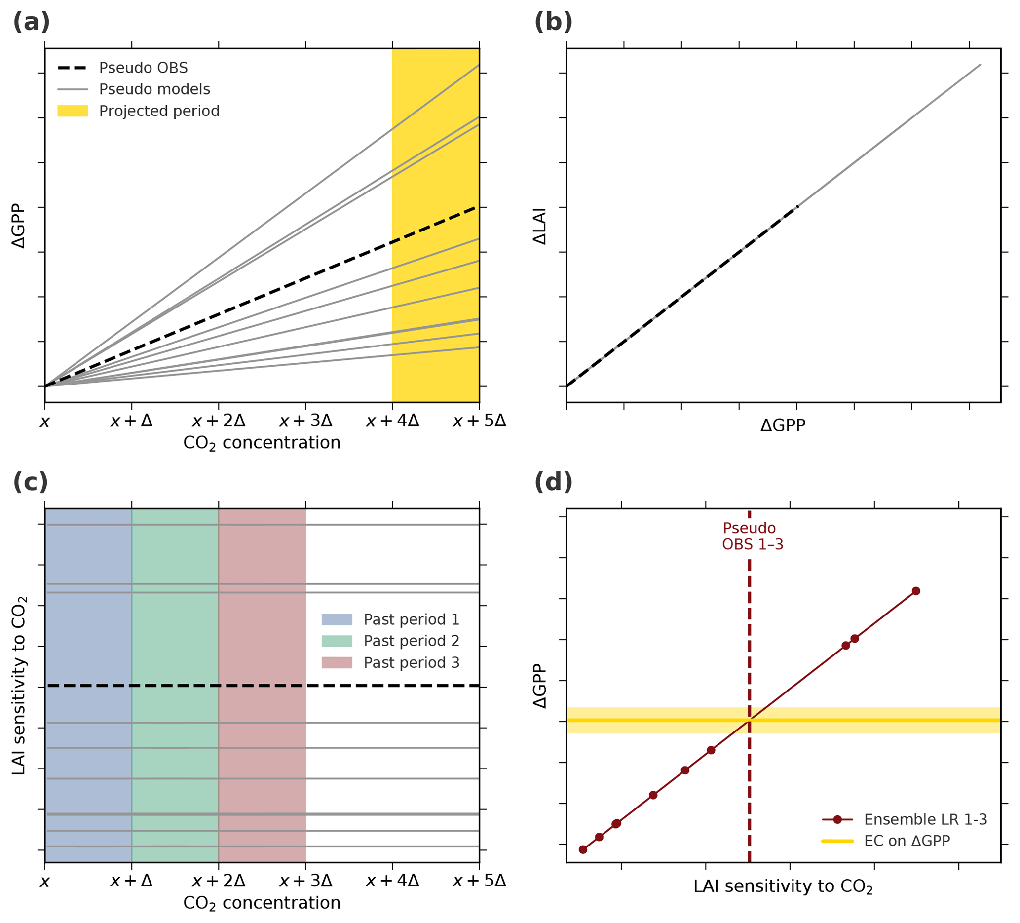
Figure A5 Thought experiment to examine the applicability of the EC analysis assuming an idealized linear–linear behavior of the system (Case 1, Table A1). (a) Changes in GPP relate linearly to changes in CO₂ concentration. The yellow band marks the projection period of interest, i.e., the period of CO₂ concentration from x+4Δ to x+5Δ. (b) Changes in LAI relate linearly to changes in GPP. The parameterization in the linear functions for pseudo observations (dashed black line) as well as models (solid gray lines) is determined randomly for each model. (c) The diagnostic variable, LAI sensitivity to CO₂, remains constant with increasing CO₂ as a consequence of the overall linear characteristics of the system. The colored bands indicate three “past” periods from x to x+Δ (blue), x+Δ to x+2Δ (green), and x+2Δ to x+3Δ (red). (d) Linear relationships among the pseudo model ensembles (Ensemble LR 1–3 on top of each other, red) between LAI sensitivity to CO₂ of the three past periods and ΔGPP from the projected period. Red dots mark different models and the dashed line represents associated pseudo observations for all three historical periods. The solid yellow line depicts the constant EC on projected ΔGPP irrespective of the past period.

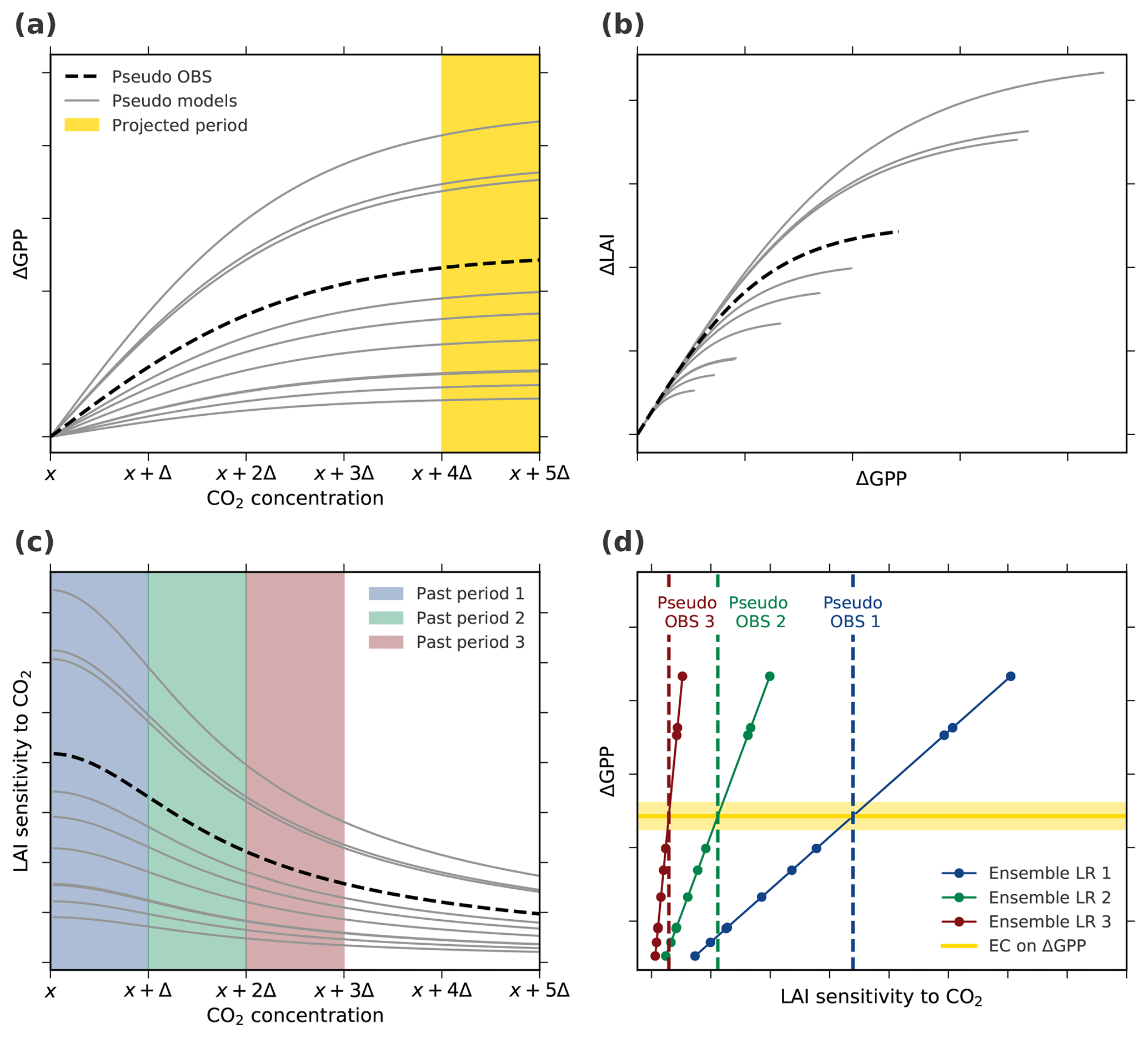
Figure A6 Thought experiment to examine the applicability of the EC analysis assuming an idealized nonlinear–nonlinear behavior of the system (Case 4, Table A1). (a) ΔGPP decreases with increasing CO₂ concentration (described by a hyperbolic tangent function). The yellow band marks the projected period of interest, i.e., the period of CO₂ concentration from x+4Δ to x+5Δ. (b) Also, ΔLAI decreases with increasing GPP (described by a hyperbolic tangent function). The parameterization in the hyperbolic tangent functions for pseudo observations (dashed black line) as well as models (solid gray lines) is determined randomly for each model. (c) The diagnostic variable, LAI sensitivity to CO₂, decreases with increasing CO₂ as a consequence of the overall saturating characteristics of the system. The colored bands indicate three “past” periods from x to x+Δ (blue), x+Δ to x+2Δ (green), and x+2Δ to x+3Δ (red). (d) Linear relationships among the pseudo model ensembles (Ensemble LR, colored lines) between LAI sensitivity to CO₂ of the three past periods and ΔGPP from the projected period. Colored dots mark different models and the dashed lines represent associated pseudo observations for the respective historical period. The solid yellow line depicts the constant EC on projected ΔGPP irrespective of the past period.

Table A1 Overview of four possible cases of interaction between forcing, nonobservable, and observable identified in the thought experiment: all linear, all nonlinear, and two mixed cases.