the Creative Commons Attribution 4.0 License.
the Creative Commons Attribution 4.0 License.
 | 24 May 2018
Bias correction of surface downwelling longwave and shortwave radiation for the EWEMBI dataset
Many meteorological forcing datasets include bias-corrected surface downwelling longwave and shortwave radiation (rlds and rsds). Methods used for such bias corrections range from multi-year monthly mean value scaling to quantile mapping at the daily timescale. An additional downscaling is necessary if the data to be corrected have a higher spatial resolution than the observational data used to determine the biases. This was the case when EartH2Observe (Calton et al., 2016) rlds and rsds were bias-corrected using more coarsely resolved Surface Radiation Budget (Stackhouse Jr. et al., 2011) data for the production of the meteorological forcing dataset EWEMBI (Lange, 2016). This article systematically compares various parametric quantile mapping methods designed specifically for this purpose, including those used for the production of EWEMBI rlds and rsds. The methods vary in the timescale at which they operate, in their way of accounting for physical upper radiation limits, and in their approach to bridging the spatial resolution gap between E2OBS and SRB. It is shown how temporal and spatial variability deflation related to bilinear interpolation and other deterministic downscaling approaches can be overcome by downscaling the target statistics of quantile mapping from the SRB to the E2OBS grid such that the sub-SRB-grid-scale spatial variability present in the original E2OBS data is retained. Cross validations at the daily and monthly timescales reveal that it is worthwhile to take empirical estimates of physical upper limits into account when adjusting either radiation component and that, overall, bias correction at the daily timescale is more effective than bias correction at the monthly timescale if sampling errors are taken into account.
- Article
(4559 KB) - Full-text XML
- BibTeX
- EndNote


High-quality observational datasets of surface downwelling radiation are of interest in many fields of climate science, including energy budget estimation (Kiehl and Trenberth, 1997; Trenberth et al., 2009; Wild et al., 2013) and climate model evaluation (Garratt, 1994; Ma et al., 2014; Wild et al., 2015). As part of so-called climate or meteorological forcing datasets such as those generated within the Global Soil Wetness Project (Zhao and Dirmeyer, 2003), at Princeton University (Sheffield et al., 2006), and within the Integrated Project Water and Global Change (Weedon et al., 2011), the longwave and shortwave components of surface downwelling radiation (abbreviated as rlds and rsds or just longwave and shortwave radiation in the following) are used to correct model biases in climate model output (Cannon, 2017; Hempel et al., 2013; Iizumi et al., 2017) and drive simulations of climate impacts, for example (Chang et al., 2017; Ito et al., 2017; Krysanova and Hattermann, 2017; Müller Schmied et al., 2016; Veldkamp et al., 2017).
These meteorological forcing datasets are global, long-term meteorological reanalysis datasets such as those produced by the National Centers for Environmental Prediction – National Center for Atmospheric Research (Kalnay et al., 1996; Kistler et al., 2001) and the European Centre for Medium-Range Weather Forecasts (Dee et al., 2011; Uppala et al., 2005), refined by bias correction using global, gridded observational data. For the components of surface downwelling radiation, such a bias correction is often necessary because observations of these variables are not assimilated in the reanalyses, which makes them subject to modelling biases of land–atmosphere interactions and cloud processes, for example (Kalnay et al., 1996; Ruane et al., 2015).
Different approaches are adopted in order to carry out these bias corrections. Weedon et al. (2011, 2014) apply indirect corrections at the monthly timescale using near-surface air temperature observations for rlds and observations of atmospheric aerosol loadings and cloudiness for rsds. Sheffield et al. (2006) directly rescale rlds and rsds to match observed multi-year monthly mean values. Ruane et al. (2015) directly adjust distributions of daily mean rsds. The observational dataset commonly used for such direct adjustments of rlds and rsds is the Surface Radiation Budget (SRB) dataset assembled by the National Aeronautics and Space Administration (NASA) and the Global Energy and Water Exchanges project (Stackhouse Jr. et al., 2011).
Another meteorological forcing dataset, the EartH2Observe, WFDEI and ERA-Interim data Merged and Bias-corrected for ISIMIP (Lange, 2016), was recently assembled to be used as the reference dataset for bias correction of global climate model output within the Inter-Sectoral Impact Model Intercomparison Project phase 2b (Frieler et al., 2017). The surface downwelling longwave and shortwave radiation data included in EWEMBI are based on daily rlds and rsds from the climate forcing dataset compiled for the EartH2Observe project (Calton et al., 2016). In order to reduce deviations of E2OBS rlds and rsds statistics from the corresponding SRB estimates in particular over tropical land (Dutra, 2015), for EWEMBI, the former were bias-adjusted to the latter at the daily timescale using two newly developed parametric quantile mapping methods.
These methods are conceptually similar to the Ruane et al. (2015) method, which fits beta distributions to reanalysed and observed daily mean rsds for every calendar month, thereby accounting for upper and lower physical limits of rsds using the multi-year monthly maximum value as the upper and zero as the lower limit of the distribution, and then uses quantile mapping to adjust the distributions. In contrast to Ruane et al. (2015), the methods developed to adjust E2OBS rlds and rsds for EWEMBI applies moving windows to estimate beta distribution parameters for every day of the year. This precludes discontinuities at the turn of the month (Gennaretti et al., 2015; Rust et al., 2015) and promises a better bias correction where the seasonality of radiation is very pronounced such as for rsds at high latitudes. Also, the new methods estimate the physical upper limits of rlds and rsds differently, acknowledging that these limits are necessarily greater than or equal to the greatest value observed during any fixed period. Lastly, while Ruane et al. (2015) linearly interpolate SRB rsds from its natural horizontal resolution of 1.0∘ to the 0.5∘ reanalysis grid prior to bias correction, the new methods aggregate the E2OBS data from their original 0.5∘ grid to the 1.0∘ SRB grid, where the bias correction is then carried out, and disaggregates these aggregated and bias-corrected data back to the E2OBS grid. Depending on the disaggregation method, this approach promises to generate bias-corrected data with more realistic temporal as well as spatial variability.
The new methods are comprehensively described and cross validated in this article. Moreover, several modifications of the new methods are tested here that differ in how they handle the spatial resolution gap between the E2OBS and SRB grids, and how they account for the physical upper limits of rlds and rsds. Also included are bias correction methods that operate at the monthly timescale in order to test if bias correction of daily or monthly mean values yields better overall cross-validation results. The lessons learned from these analyses shall benefit bias corrections of surface downwelling radiation to be carried out in future generations of climate forcing datasets.
2.1 E2OBS
The EartH2Observe (Calton et al., 2016; Dutra, 2015) daily mean rlds and rsds data bias-corrected for EWEMBI cover the whole globe on a regular 0.5∘ × 0.5∘ latitude–longitude grid and span the 1979–2014 time period. Over the ocean, E2OBS rlds and rsds are identical to bilinearly interpolated ERA-Interim (Dee et al., 2011) rlds and rsds. Over land, they are identical to WATCH Forcing Data methodology applied to ERA-Interim reanalysis data (Weedon et al., 2014) rlds and rsds. WFDEI rlds, in turn, is identical to bilinearly interpolated ERAI rlds, adjusted for elevation differences between the ERAI and Climatic Research Unit (Harris et al., 2013) grids. WFDEI rsds is identical to bilinearly interpolated ERAI rsds bias-corrected at the monthly timescale using CRU TS3.1/3.21 mean cloud cover and considering effects of interannual changes in atmospheric aerosol optical depths (Weedon et al., 2010, 2011, 2014).
2.2 SRB
The observational data used for the bias correction of E2OBS daily mean rlds and rsds for EWEMBI were the NASA–GEWEX Surface Radiation Budget (Stackhouse Jr. et al., 2011) primary-algorithm estimates of daily mean rlds and rsds from the latest SRB releases available at the time, which were release 3.1 for rlds and release 3.0 for rsds. These data cover the whole globe on a regular 1.0∘ × 1.0∘ latitude–longitude grid and span the July 1983–December 2007 time period. For bias correction and cross validation, a 24-year subsample of these data that spans the December 1983–November 2007 time period was used and is used here. Additional data from the adjacent months November 1983 and December 2007 are employed for computations of running mean values. The SRB estimates of rlds and rsds are based on satellite-derived cloud parameters and ozone fields, reanalysis meteorology, and a few other ancillary datasets. Due to a lack of satellite coverage during most of the July 1983–June 1998 time period over an area centred at 70∘ E, SRB data artefacts are present over the Indian Ocean (https://gewex-srb.larc.nasa.gov/common/php/SRB_known_issues.php, last access: 18 May 2018; see Figs. 2–4, 7). Every SRB grid cell contains exactly four E2OBS grid cells.
For the reader who is is not familiar with the concepts of quantile mapping and/or statistical downscaling, a short introduction including definitions of relevant terms is given in Appendix A. The parametric quantile mapping methods introduced in the following are named according to the scheme BCvtpx, where are used to distinguish between methods for longwave and shortwave radiation () operating at the daily and monthly timescales () using basic and advanced distribution types or parameter estimation techniques (). Index is used for variants of these methods that differ in how they handle the spatial resolution gap between the SRB and E2OBS grids. For the BCvtp0 methods, the SRB data are spatially bilinearly interpolated to the E2OBS grid and the E2OBS data are then bias-corrected using these interpolated SRB data; this is to mimic the Ruane et al. (2015) approach. For bias correction with the BCvtp1 methods, E2OBS data are spatially aggregated to the SRB grid, and the aggregated data are then bias-corrected and the resulting data disaggregated back to the E2OBS grid; this approach was used to produce the EWEMBI radiation data. Lastly, the BCvtp2 methods adjust mean values and variances at the E2OBS grid such that mean values and variances of spatial aggregates to the SRB grid match the corresponding SRB estimates while the sub-SRB-grid-scale spatial structure of mean values and variances present in the original E2OBS data is retained; this is to overcome the variability deflation induced by the other two approaches. Since the BCvtp0 and BCvtp2 methods are based on the BCvtp1 methods, the latter are introduced first. Readers who are merely interested in how the EWEMBI radiation data were produced are informed that methods BClda1 and BCsda1 were used for that purpose.
3.1 Bias correction at the SRB grid scale
For the BCvtp1 methods, daily mean E2OBS rlds and rsds are first aggregated to the SRB grid using a first-order conservative remapping scheme (Jones, 1999). The conservative remapping ensures that each aggregated value is the grid-cell area-weighted mean of the underlying four E2OBS values. The methods of bias correction of these aggregated values are described in the following. The method used for the subsequent disaggregation to the E2OBS grid is described in Sect. 3.1.3.
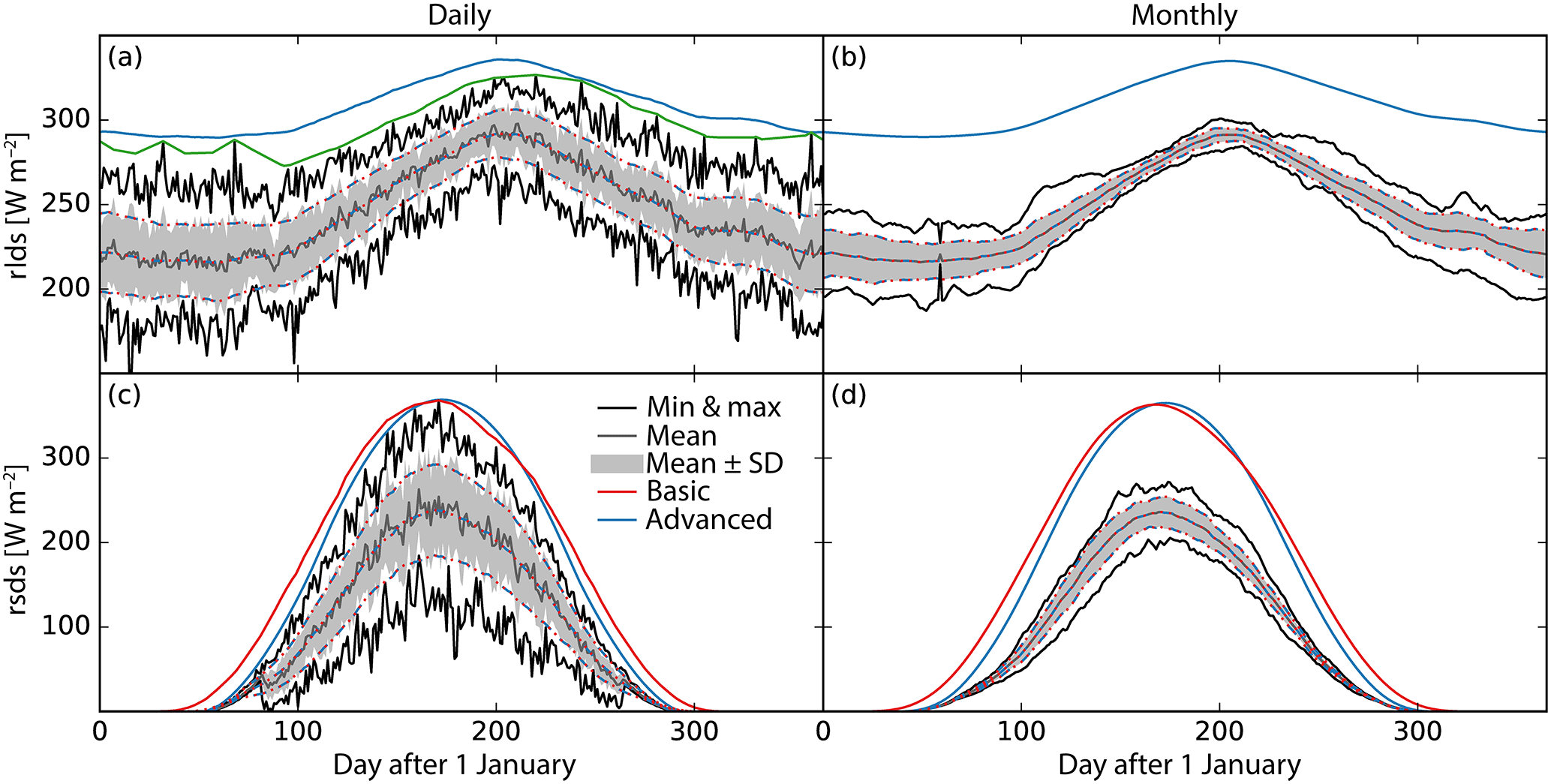
Figure 1Estimation of parameters of quantile mapping methods used for the bias correction of longwave (a, b) and shortwave (c, d) radiation at the daily (a, c) and monthly (b, d) timescales. This example is based on SRB daily mean rlds and rsds data from 79.5∘ N, 12.5∘ E and the December 1983–November 2007 time period. Climatological distribution parameters are estimated based on empirical 24-year mean values (dark grey), standard deviations (light grey range around mean values), and minimum and maximum values (black) of daily mean (a, c) and 31-day running mean (b, d) radiation computed for every day of the year. The distribution parameters estimated for the basic (red) and advanced (blue) bias correction methods (see Table 1) include mean values and standard deviations (dotted red, dashed blue), and upper bounds (solid red, solid blue) where beta distributions are used. Note that the basic and advanced estimates of mean values and standard deviations only differ in panel (c) near the beginning and end of polar night (see Table 1). The green line in panel (a) represents 25-day running mean values of 25-day running maximum values of 24-year maximum values of daily mean rlds, which are used to estimate the upper bounds of the climatological beta distributions used by the BClda1 method (solid blue line in panel a). The lower bounds of all climatological beta distributions are set to zero.
The BCvtp1 methods use parametric transfer functions of the form , where and are climatological cumulative distribution functions (CDFs) of aggregated E2OBS and SRB data, respectively. The CDFs are estimated individually for every SRB grid cell and day of the year (Fig. 1). In order to quantify the extent to which bias correction results benefit from explicitly accounting for physical radiation limits, the basic and advanced methods BCltb1 and BClta1 for longwave radiation use normal and beta distributions, respectively. For shortwave radiation, the relevance of physical limits is less questionable, given that the lower limit of zero matters at least during polar night, and that the solar radiation incident upon land and ocean surfaces is limited by the solar radiation incident upon the top of the atmosphere (see Fig. 1). Therefore, all BCstp1 methods use beta distributions and the basic and advanced methods only differ in how they estimate the beta distribution parameters (see Fig. 1, Table 1).
Table 1Distribution types and parameter estimation methods of bias correction methods BCvtp1 for day d of the year (see Fig. 1). Please note that the lower bounds of all climatological beta distributions are set to zero and that 24-year statistics are replaced by 12-year statistics for cross validation.
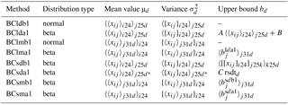
xij is the daily mean rlds (for BCltp1) or rsds (for BCstp1) on day j of year i. Brackets 〈 ⋅〉, { ⋅}, and [ ⋅] denote the calculation of sample mean values, variances, and maximum values, respectively. Bracket subscripts i24, j31d, j25d, and j25d* indicate that these sample statistics are calculated over years , over days , over days , and over days with , respectively. Constants A, B, and C are determined by , , and , respectively.
3.1.1 Bias correction at the daily timescale
The parameters of the climatological CDFs and are estimated based on empirical multi-year mean values, variances, and maximum values of daily mean radiation from the December 1983–November 2007 time period. Data from the whole period were used for the production of EWEMBI rlds and rsds. Data from some half of the period (see Sect. 4.1) are used for cross validation in this study.
For shortwave radiation, the basic daily bias correction method is designed to resemble the method outlined by Ruane et al. (2015). BCsdb1 estimates mean values and variances of climatological beta distributions by 25-day running mean values of multi-year daily mean values and variances, respectively, and their upper bounds by 25-day running mean values of 25-day running maximum values of multi-year maximum values of daily mean rsds (solid red line in Fig. 1c). The idea behind this upper-bound estimate is that 25-day running maximum values of multi-year maximum values of daily mean rsds resemble the multi-year monthly maximum values of daily mean rsds used by Ruane et al. (2015). Please note that using the same window length for the running maximum calculation and the additional smoothing ensures that the resulting upper bounds are always greater than or equal to the multi-year maximum values of daily mean rsds.
The BCsda1 method employs the climatology of daily mean shortwave insolation at the top of the atmosphere (rsdt; see Appendix B for how rsdt is calculated in this study) for the upper-bound estimation. This is motivated by rsds being limited by rsdt in most locations and seasons, which suggests that the annual cycle of the upper bound of daily mean rsds has a similar shape as the climatology of daily mean rsdt. Therefore, method BCsda1 uses a rescaled daily mean rsdt climatology as the upper-bound climatology of daily mean rsds (solid blue line in Fig. 1c). The rescaling is performed with the smallest possible factor that guarantees that the resulting upper bounds are greater than or equal to the multi-year maximum values of daily mean rsds on all days of the year with rsdt ≥ 50 W m−2. An extension of this guarantee to days of the year with lower rsdt would inflate the rescaling factor because during dusk and dawn of polar night, rsds can exceed rsdt due to diffuse radiation coming in from lower latitudes. Therefore, on days of the year with rsdt < 50 W m−2, the maximum of the rescaled rsdt and the empirical multi-year maximum daily mean rsds is used as the upper rsds bound. Mean values and variances of the climatological beta distributions of the BCsda1 method are estimated by running mean values of multi-year daily mean values and variances, respectively. The window length used for these running mean calculations is 25 days by default. On days that are fewer than 13 days away from the beginning or end of polar night (as defined by daily mean rsdt going to zero), the window length is shortened to 2n+1, where n is the number of days between the day in question and the beginning or end of polar night.
For longwave radiation, both the basic and the advanced daily bias correction methods use 25-day running mean values of multi-year daily mean values and variances to estimate climatological mean values and variances, respectively. The upper bounds used by BClda1 are not estimated by the often rather un-smooth 25-day running mean values of 25-day running maximum values of 24-year maximum values of daily mean rlds (solid green line in Fig. 1a) but by a suitably shifted and rescaled mean value climatology (solid blue line in Fig. 1a; formulas in Table 1).
Since the choice of the window length used for all the running mean and maximum value calculations mentioned above is somewhat arbitrary, the window length dependence of the overall performances of the BCvda1 methods is investigated in Appendix D. Sensitivities are found to be very low for window lengths between 10 and 40 days.
3.1.2 Bias correction at the monthly timescale
In order to mimic a bias correction at the monthly timescale as was performed by Sheffield et al. (2006), for example, the BCvmp1 methods bias-correct 31-day running mean values and then rescale each daily value by the corrected-to-uncorrected ratio of the respective 31-day running mean value.
Mean values and variances of the climatological CDFs and of 31-day running mean values are simply estimated by 24-year (or 12-year for cross validation) daily mean values and variances of 31-day running mean values, respectively, with 29 February values replaced by averages of 28 February and 1 March values.
Upper bounds of beta distributions are estimated by 31-day running mean values of the upper bounds of the corresponding CDFs and of daily mean radiation (see Fig. 1, Table 1) because 31-day running mean values of multi-year maximum values of daily mean radiation are mathematically always greater than or equal to multi-year maximum values of 31-day running mean radiation. The resulting upper bounds are typically much larger than observed 24-year maximum monthly mean radiation (see Fig. 1d) because 31 consecutive days of daily mean radiation at the respective physical upper limit are very unlikely to occur in reality.
3.1.3 Disaggregation to the E2OBS grid
In principle, the disaggregation of aggregated and bias-corrected E2OBS data from the SRB to the E2OBS grid can be carried out in various ways. The simplest approach would arguably be a mere interpolation, which is disadvantageous since it ignores the sub-SRB-grid-scale spatial variability present in the original E2OBS data. Probabilistic disaggregation methods that are designed to retain that variability (Sheffield et al., 2006), are impractical if, as in the present case, the purpose of the disaggregation is the production and publication of a dataset because all variants of the dataset that can potentially be generated by a probabilistic algorithm are, as long as all conceivable constraints have been incorporated in the algorithm, equally plausible candidates for the one dataset to be published. Therefore, not a probabilistic but the following deterministic disaggregation approach was used for the production of EWEMBI rlds and rsds and is adopted here for all BCvtp1 methods.
First, E2OBS-grid-scale upper bounds of daily mean radiation are estimated by bilinearly interpolated maximum values of the climatological upper bounds of SRB all-sky and clear-sky radiation, which in turn are estimated using the BClda1 method for rlds and the BCsda1 methods for rsds (see Table 1 and blue lines in Fig. 1a, c). The clear-sky radiation data are included in order to prevent the E2OBS-grid-scale upper bounds from being much lower than the real physical limits of daily mean radiation at that spatial scale, given that due to sub-SRB-grid-scale spatial variability, upper radiation bounds at the E2OBS grid scale may exceed those at the SRB grid scale.
The original daily E2OBS data are then clamped between zero and these upper bounds, and the resulting values (or their distances to their upper bounds) are rescaled day by day and SRB grid cell by SRB grid cell such that their SRB-grid-scale aggregates match the bias-corrected values. More precisely, for a fixed but arbitrary SRB grid cell and a fixed but arbitrary day, let Y denote the bias-corrected value at the SRB grid scale, wk with the area weights of the four E2OBS grid cells contained in the SRB grid cell, Xk the clamped original E2OBS data values with upper bounds bk, and Yk the bias-corrected values at the E2OBS grid scale to be computed. If , then Yk is computed according to Yk=fXk with . Otherwise Yk is computed according to with . This rescaling procedure ensures that and .
3.2 Bias correction at the E2OBS grid scale
3.2.1 The BCvtp2 methods
The disaggregation method introduced above corrects the original E2OBS values from the four E2OBS grid cells contained in one SRB grid cell as if they must all be too low (high) if their area-weighted average is too low (high). This implicit assumption is questionable since it rules out the possibility that the area-weighted average is too low because one of the four values is much too low while the others are slightly too high, to give just one example. A statistical manifestation of this problem is illustrated and discussed in Sect. 4.2.
The assumption does not need to be made if the bias correction is carried out directly at the E2OBS grid. With target distributions fixed at the SRB grid, target distributions at the E2OBS grid can be defined such that the bias-corrected data have the SRB-grid-scale target distributions and the sub-SRB-grid-scale structure of the original E2OBS data. For parametric bias correction methods such as those introduced above, this can be achieved via suitable definitions of the parameters of the E2OBS-grid-scale target distributions. Here, for every BCvtp1 method, a corresponding BCvtp2 method is defined to operate at the same temporal scale and to use the same source (at the E2OBS grid) and target (at the SRB grid) distribution type and parameter estimation technique (see Table 1). E2OBS-grid-scale target climatologies of mean values, variances, and (where necessary) upper bounds are defined as follows.
The mean value estimates of the original E2OBS data are shifted by a common offset per SRB grid cell and day of the year to obtain the E2OBS-grid-scale target mean values. The offsets are chosen such that the E2OBS-grid-scale target mean values aggregated to the SRB grid match the corresponding SRB mean value estimates. E2OBS data bias-corrected using these E2OBS-grid-scale target mean values have SRB-grid-scale aggregates that match the SRB-grid-scale target mean values because (i) the aggregation is a linear operation and (ii) the mean value of a linear combination of random variables is equal to the same linear combination of the mean values of these random variables.
To obtain the E2OBS-grid-scale target variances, the variance estimates of the original E2OBS data are rescaled by a common (to all four E2OBS grid cells contained in one SRB grid cell) factor fij per day i of the year and SRB grid cell j. For the derivation of the formula for fij let Yijk (and Xijk) denote random variables representing bias-corrected (and original) E2OBS data from day i of the year and E2OBS grid cells contained in SRB grid cell j. Then the estimated variance of the SRB-grid-scale aggregate of Yijk can be expanded to
where wjk is the area weight of E2OBS grid cell jk with for all j, Cov(Yijk,Yijl) is the estimated covariance of Yijk and Yijl, Cor(Yijk,Yijl) is the estimated Pearson correlation of Yijk and Yijl, and Var(Yijk) is the estimated variance of Yijk. A bias correction would be deemed successful if the left-hand side of Eq. (1) was equal to the estimated variance of Zij, the SRB data from day i of the year and grid cell j. On the right-hand side of Eq. (1), fij Var(Xijk) can be substituted for Var(Yijk) by definition of the scaling factors, and Cor(Yijk,Yijl) can be approximated by Cor(Xijk,Xijl) since quantile mapping preserves ranks and therefore rank correlations and therefore approximately Pearson correlations. The variance scaling factors fij for method BCvtp2 are therefore calculated based on
where the variances are estimated using the respective BCvtp1 approach (see Table 1), and the Pearson correlations are estimated by inversely Fisher-transformed 25-day running mean values of Fisher-transformed 24-year daily Pearson correlations of daily (for BCvdp2) or 31-day running mean (for BCvmp2) radiation data. The Fisher transformations are invoked here in order to approximately account for correlation value-dependent sampling error intervals (Fisher, 1915, 1921).
The E2OBS-grid-scale target upper bounds are calculated in the same way as the E2OBS-grid-scale target mean values. This way, the latter rarely exceed the former. Where they do, the latter are reduced to 99 % of the former. For longwave (shortwave) radiation, such reductions are necessary in four (11 % of all) E2OBS grid cells on an average of 15 % (5 %) of all days of the year.
Furthermore, in order to obtain realistic E2OBS-grid-scale target beta distributions, the E2OBS-grid-scale target variances calculated using Eq. (2) are limited to 40 % of µ(b−µ), where µ and b are the E2OBS-grid-scale target mean values and upper bounds, respectively. This limit is imposed because (i) the variance σ2 of a random variable taking values from within the interval [a,b] can generally not be greater than if µ is the random variable's mean value; (ii) if that random variable is beta distributed and then the probability density function is U shaped (Wilks, 1995), which is considered unrealistic for climatological distributions of rlds and rsds; and (iii) has an empirical upper limit of about 40 % in the original E2OBS radiation data. The 40 % condition is never met for longwave radiation whereas for shortwave radiation it is met in 14 % of all E2OBS grid cells on an average of 2 % of all days of the year.
3.2.2 The BCvtp0 methods
For the BCvtp0 methods, daily SRB data are first bilinearly interpolated to the E2OBS grid. The E2OBS data are then bias-corrected directly at the E2OBS grid using the interpolated SRB data and transfer functions defined exactly as for the respective BCvtp1 method.
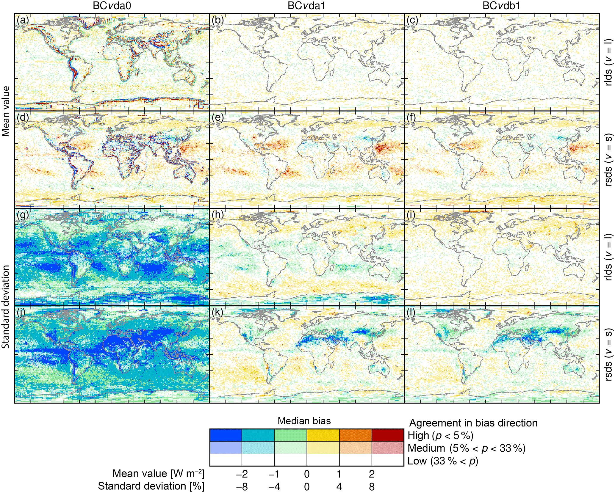
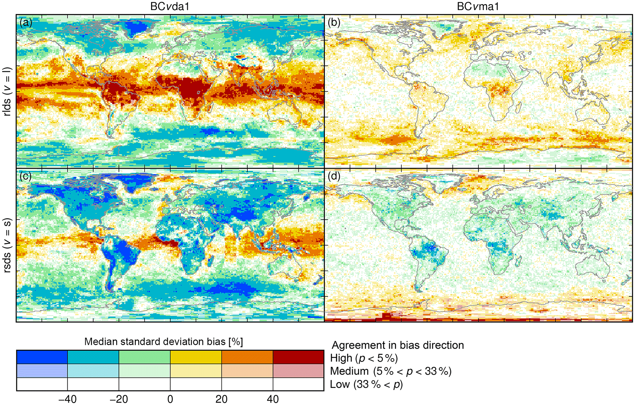
Figure 2Biases relative to SRB in mean values (a–f) and standard deviations (g–l) of spatially aggregated (to the SRB grid) daily mean longwave (a–c, g–i) and shortwave (d–f, j–l) radiation after bias correction with methods BCvda0 (left), BCvda1 (middle), and BCvdb1 (right). The biases are calculated individually for each calendar month (January to December) and calibration data sample (every1st, every2nd) pooling SRB and corrected E2OBS data from all years of the corresponding validation data sample (every2nd, every1st, respectively) and omitting shortwave radiation data from months with monthly mean rsdt less than 1 W m−2 (see Appendix B and Fig. D1c). Depicted are median and agreement in direction (sign of bias) of these individual biases, represented by hue and saturation of a grid cell's colour, respectively. Categories of agreement in bias direction are defined based on one-sided p values obtained from modelling underestimations and overestimations for individual calendar months and validation data samples as outcomes of independent 50/50 Bernoulli trials. More saturated colours indicate higher statistical significance of biases remaining after bias correction.
In the following, the bias correction methods introduced above are cross validated at the SRB grid scale (Sect. 4.1), and their disaggregation performance is assessed by comparing sub-SRB-grid-scale spatial variability before and after bias correction (Sect. 4.2).
4.1 Cross validation at the SRB grid scale
For the cross validation against SRB data, 24 years worth of overlapping E2OBS and SRB data are divided into two 12-year samples of which the first one is used to calibrate and the second one to validate the method. Common practice would be to use data from the first and second half of the 24-year period to define these samples. However, due to climate change this definition may yield calibration and validation data samples that differ statistically. These differences in turn, which are essentially climate change signals, may differ in extent between the E2OBS and SRB data. Switanek et al. (2017) have shown that such differences in climate change signals may then dominate cross-validation metrics and thereby distort the comparative validation of bias correction methods. In order to minimise this climate change impact on cross-validation results, here, calibration and validation data samples are composed of data from all odd years and all even years or vice versa, respectively. The samples are accordingly labelled every1st and every2nd.
Please note that results for BCvtp2 are not shown or discussed in this section because BCvtp1 and BCvtp2 produce virtually identical data at the SRB grid scale.
4.1.1 BCvtp0 vs. BCvtp1
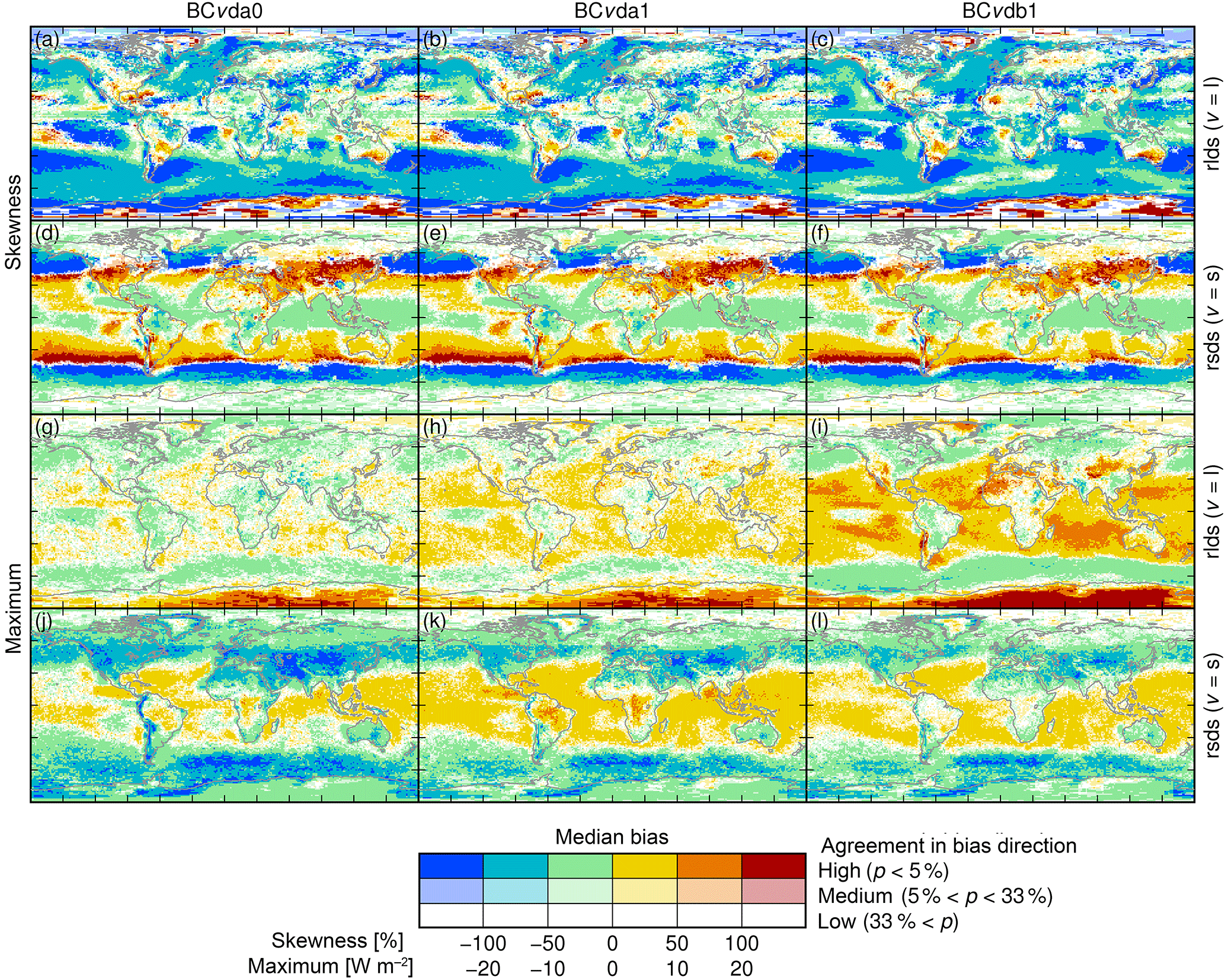
The first question addressed here is how the bilinear spatial interpolation of SRB data to the E2OBS grid before bias correction with the BCvtp0 methods impacts the distribution of bias-corrected rlds and rsds values at the SRB grid scale. To quantify these impacts, biases in multi-year daily mean values, standard deviations, and maximum values remaining after bias correction with methods BCvda0 and BCvda1 are compared in the left and middle columns of Figs. 2 and 3.
Since linear interpolation always yields values that are intermediate to the values at the interpolation knots it is expected that daily SRB data bilinearly interpolated to the E2OBS grid and then aggregated back up to the SRB grid will be more smooth overall both in space and time than the original SRB data. Manifestations of the increased smoothness in time are the more negative biases of standard deviations (Fig. 2) and maximum values (Fig. 3) remaining after bias correction with BCvda0 than with BCvda1. Standard deviations after bias correction with BCvda0 in particular are negatively biased by more than 4 % (median over calendar months × validation data samples) in most regions. In mountainous and therefore spatially heterogeneous regions, multi-year monthly mean radiation is also changed significantly by the interpolation, with median biases over calendar months × validation data samples remaining after bias correction with BCvda0 exceeding 2 W m−2 in many such places (Fig. 2).
4.1.2 BCvtax vs. BCvtbx
Next is an assessment of how the treatment of the upper bound of the distributions estimated by the BCvdp1 methods impacts the distribution of bias-corrected rlds and rsds values at the SRB grid scale. To quantify these impacts, biases in multi-year daily mean values, standard deviations, and maximum values remaining after bias correction with methods BCvda1 and BCvdb1 are compared in the middle and right columns of Figs. 2 and 3.
For longwave radiation, the basic method BCldb1 assumes normally distributed values and therefore does not account for any upper physical limit of rlds whereas the advanced method BClda1 assumes the existence of such a limit and estimates it empirically. Figure 3 shows that the advanced method generally yields a better correction of 12-year maximum values. In contrast, standard deviations are slightly better corrected by the basic method and mean values are equally well corrected by both methods (Fig. 2).
For shortwave radiation, both the basic and the advanced method empirically estimate upper physical limits of rsds and take these into account in the form of upper bounds of beta distributions. The limit estimates are based on downwelling shortwave radiation at the surface and at the top of the atmosphere for BCsda1, and on rsds only for BCsdb1. Figure 3 shows that the basic method generally yields a better correction of 12-year maximum values. Standard deviations and mean values are also slightly better corrected by BCsda1 than by BCsdb1 (Fig. 2).
4.1.3 BCvdpx vs. BCvmpx
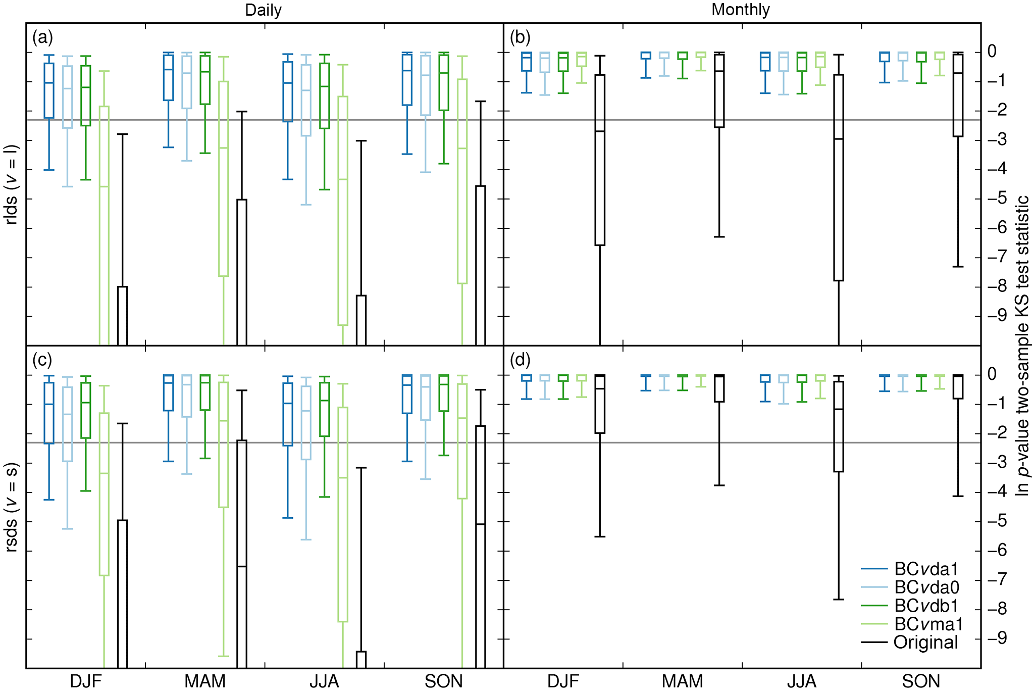
Figure 5Overall performance of bias correction methods BCvda1, BCvda0, BCvdb1, and BCvma1 for longwave (top) and shortwave (bottom) radiation at the daily (left) and monthly (right) timescales as quantified by p values of two-sample Kolmogorov–Smirnov test statistics of the respective E2OBS and SRB data before (black) and after (colours) bias correction (see Appendix C; greater p values indicate stronger agreement of E2OBS and SRB distributions). The p values are determined individually for each grid cell, season, and calibration data sample, with all corresponding values pooled into one distribution and omitting shortwave radiation data from months with average rsdt less than 1 W m−2. The horizontal lines of each box–whisker plot represent the 90th, 75th, 50th, 25th, and 10th (from top to bottom) grid-cell area-weighted percentiles of the natural logarithms of these p values over calibration data sample (1sthalf, 2ndhalf), latitude, and longitude. The grey horizontal line marks the p=10 % significance level.

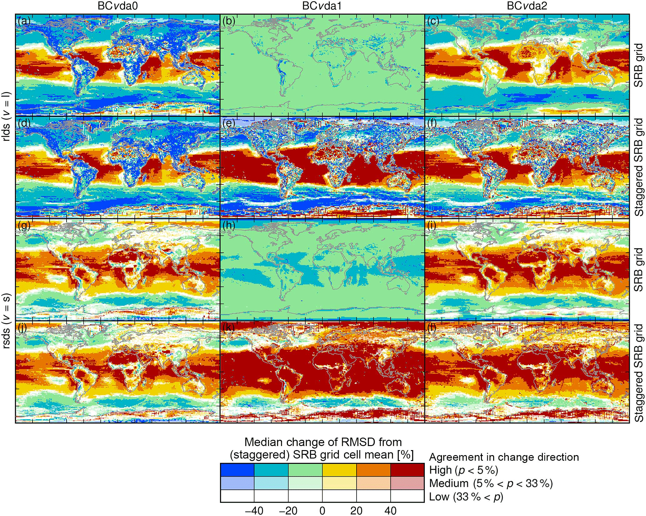
Figure 7Relative change by bias correction with methods BCvda0 (left), BCvda1 (middle), and BCvda2 (right) of the root-mean-square deviation (RMSD) of daily mean E2OBS-grid-scale longwave (a–f) and shortwave (g–l) radiation from the aggregated SRB-grid-scale values based on 1∘ grid cells of the SRB grid (a–c, g–i) and the staggered SRB grid (d–f, j–l; see text). For every 1∘ grid cell and calendar month, the RMSDs are calculated using original or bias-corrected E2OBS data from the four 0.5∘ grid cells contained in the 1∘ grid cell, pooling data from the entire December 1983–November 2007 time period and omitting shortwave radiation data from months with average rsdt less than 1 W m−2. Depicted are median and agreement in the direction of monthly RMSD changes by bias correction (same colouring scheme as in Fig. 2). Very similar results are obtained for the corresponding basic bias correction methods.
Next is a comparative cross validation of methods BCvdpx and BCvmpx operating at the daily and monthly timescales, respectively. The cross validation itself is also performed at the daily and monthly timescales based on statistics of daily and monthly mean radiation, respectively. A joint assessment of these cross validations shall reveal whether bias correction at the daily or monthly timescale is better overall.
By design, the BCvdpx and BCvmpx methods are equally good at correcting multi-year mean values of daily mean radiation. However, both day-to-day and year-to-year variability are expected to be differently well corrected by the methods operating at different timescales. Since day-to-day variability is (not) explicitly adjusted by the methods operating at the daily (monthly) timescale, the BCvdpx methods are expected to perform better at the daily timescale than the BCvmpx methods. The year-to-year variability, however, is explicitly corrected by the BCvmpx methods and it is not by the BCvdpx methods because daily data from different years are pooled before quantile mapping is carried out at the daily timescale. Consequently, biases in interannual standard deviations of monthly mean radiation are much larger after bias correction with BCvda1 than with BCvma1 (Fig. 4), and the BCvmpx methods are generally expected to perform better at the monthly timescale than the BCvdpx methods.
In order to assess whether bias correction at the daily or monthly timescale is more effective overall, a performance measure is needed that is comparable across timescales. Common performance measures of distribution adjustments at individual timescales are the two-sample Kolmogorov–Smirnov (KS) and Kuiper's two-sample test statistics. While Kuiper's test is equally sensitive to CDF differences at all quantiles, the KS test is more sensitive at the median than in the tails. A straightforward comparison of these test statistics across timescales is not very meaningful because sample sizes at the daily and monthly timescales differ by a factor of 30, which implies that the same value of a test statistic has different statistical significance at the daily and monthly timescales. A better comparability can be achieved by comparing the test statistic's p value, which represents the statistical significance of CDF differences. In the present cross validation, the CDFs compared are based on bias-corrected E2OBS and the corresponding SRB data, and a higher p value indicates more similar CDFs and therefore a better bias correction. For details of the calculation of p values of the two-sample KS and Kuiper's two-sample test statistics see Appendix C.
Global distributions of p values of two-sample test statistics for seasonal distributions of daily and monthly mean rlds and rsds are shown in Fig. 5 for the KS test and Fig. 6 for Kuiper's test. In accordance with expectations, both tests indicate that CDFs are generally better adjusted by BCvdpx than by BCvmpx at the daily timescale and vice versa at the monthly timescale. However, performance differences between BCvdpx and BCvmpx are clearly more significant at the daily than at the monthly timescale. This suggests that bias-correcting at the daily instead of at the monthly timescale yields bias decrements at the daily timescale that exceed bias increments at the monthly timescale. Therefore, bias correction at the daily timescale is deemed more effective overall than bias correction at the monthly timescale.
To elaborate on this further, the p=10 % significance level is marked by a grey horizontal line in all panels of Figs. 5 and 6 and is to be compared with the 10th percentiles of the global distributions of p values of the two-sample test statistics. Any coincidence of such a 10th percentile with the 10 % significance level suggests that the corresponding p-value distribution is in agreement with the null hypothesis of the respective test. Since the null hypothesis of both tests is that the samples compared are from the same underlying distribution, such a coincidence suggests that the bias correction which produced one of the samples compared worked perfectly within the limits of sampling uncertainty. Similarly, 10th percentiles of p-value distributions above (below) the 10 % significance level suggest overcorrections (undercorrections) in terms of sampling uncertainty. In that sense, the BCvtpx methods generally overcorrect at the monthly timescale and undercorrect at the daily timescale.
The KS and Kuiper's test statistics also confirm the finding of Sect. 4.1.2 that at the daily timescale, the BCvda1 methods outperform the BCvdb1 methods for longwave radiation and vice versa for shortwave radiation. This holds true for all seasons and irrespective of CDF differences being generally greater in summer and winter (DJF and JJA) than in the transition seasons (MAM and SON) both before and after bias correction. Moreover, the test statistics find both BCvda1 and BCvdb1 to outperform BCvda0 at the daily timescale, which is in line with the finding of Sect. 4.1.1 that the BCvda0 methods deflate day-to-day variability.
The fact that all BCvdp1 methods undercorrect at the daily timescale demonstrates the imperfections of these parametric quantile mapping methods. The remaining CDF differences must be linked to imperfect bias corrections of moments of higher-than-second order since multi-year mean values and standard deviations are well adjusted by design. To illustrate this, relative skewness biases remaining after bias correction with BCvdp1 are shown to exceed 50 % (median over calendar months × validation data samples) in many regions (Fig. 3). Another manifestation of the imperfections are remaining biases in the tails of the distribution of daily mean rlds and rsds. These must be larger than the remaining median biases because p values of Kuiper's test statistics for these distributions are generally larger than those of the corresponding KS test statistics.
4.2 Spatial disaggregation and sub-SRB-grid-scale spatial variability
As outlined in Sect. 3.2.1, the BCvtp1 approach to the disaggregation of bias-corrected daily mean rlds and rsds values from the SRB to the E2OBS grid scale is based on the implicit assumption that the original E2OBS values of daily mean radiation onto the four E2OBS grid cells contained in one SRB grid cell must all be too low (high) if their area-weighted average is too low (high). The four original values are then all increased (decreased) by the BCvtp1 method. In order to account for their upper (lower) physical bounds, the increases (decreases) are performed by a common scaling factor applied to the distances to these bounds. This leads to a reduction of the differences among the four values (this is necessarily true if the four bounds are equal; it is true in most cases if they are similar), i.e., to a deflation of sub-SRB-grid-scale spatial variability.
In order to illustrate and quantify the extent of this variability deflation and compare the BCvtp0, BCvtp1, and BCvtp2 methods in terms of their impact on sub-SRB-grid-scale spatial variability, the root-mean-square deviation (RMSD) of the four E2OBS-grid-scale values of daily mean radiation per SRB grid cell from their area-weighted average is calculated over all days of a given calendar month both before and after bias correction with either method. Median relative bias-correction-induced changes of these RMSDs are depicted in Fig. 7 and demonstrate that BCvda1 indeed generally deflates them, in some regions by more than 20 % (median over calendar months) for both longwave and shortwave radiation. In contrast, BCvtp0 and BCvtp2 deflate or inflate them depending on variable and region.
In an analogous manner, such RMSDs can be computed based on data from the four E2OBS grid cells contained in one staggered SRB grid cell, where the staggered SRB grid is a regular 1.0∘ × 1.0∘ latitude–longitude grid shifted by 0.5∘ latitude and 0.5∘ longitude relative to the SRB grid, i.e., every staggered SRB grid cell contains E2OBS grid cells contained in four different SRB grid cells. Median relative bias-correction-induced changes of these RMSDs are also depicted in Fig. 7. Ideally, bias-correction-induced changes of RMSDs from SRB and staggered SRB grid cell mean values would be equal. It would then be impossible to tell from their comparison whether the bias correction's target distributions were defined on the SRB or on the staggered SRB grid.
The BCvdp1 methods do not fulfil this criterion as they deflate RMSDs from SRB grid cell mean values everywhere while inflating RMSDs from staggered SRB grid cell mean values in many regions, in particular over the tropical oceans. The criterion is much better fulfilled by the BCvdp2 and BCvdp0 methods. The RMSDs are generally greater after bias correction with BCvdp2 than with BCvdp0, i.e., BCvdp2 produces data with greater sub-SRB-grid-scale spatial variability than BCvdp0. This difference is most visible for longwave radiation, for which BCvdp0 produces a stark land–sea contrast of RMSD changes with strong RMSD reductions over land whereas BCvdp0 does so to a much lesser extent. This strong deflation of sub-SRB-grid-scale spatial variability by BCvtp0 is believed to be another artefact caused by the bilinear interpolation of SRB data to the E2OBS grid.
This article introduces various parametric quantile mapping methods for the bias correction of E2OBS daily mean surface downwelling longwave and shortwave radiation using the corresponding SRB data. The quantile mapping methods differ in (i) the timescale at which they operate, (ii) if and how they take physical upper radiation bounds into account, and (iii) how they handle the spatial resolution gap between E2OBS and SRB.
A cross validation at the SRB grid scale demonstrates that statistics of daily mean radiation are better corrected by methods operating at the daily timescale than by methods operating at the monthly timescale, and vice versa for statistics of monthly mean radiation. Since these performance differences are statistically more significant at the daily than at the monthly timescale, overall, bias correction at the daily timescale is deemed more effective then bias correction at the monthly timescale.
The cross validation further suggests that it is generally worthwhile to explicitly take physical upper radiation bounds into account during quantile mapping. For shortwave radiation, different approaches to their estimation are tested. A simple approach using running maximum values is found to outperform a more complicated one based on daily mean insolation at the top of the atmosphere (rsdt). This must be due to other factors besides rsdt that influence the upper physical bounds of rsds. Atmospheric humidity is an example for such a factor: The highest rsds values usually occur under clear-sky conditions and they are higher the drier the atmosphere. Atmospheric humidity in turn is limited by the water vapour holding capacity of the atmosphere, which is controlled by atmospheric temperature. The climatology of atmospheric temperature lags behind that of rsdt. Hence, the climatology of the upper physical bounds of rsds can be expected to deviate from the rsdt climatology.
The cross validation also reveals to what extent the bilinear spatial interpolation of SRB data to the E2OBS grid prior to bias correction with the BCvtp0 methods deflates day-to-day variability. This variability deflation has a greater effect on bias correction performance than a change of if and how physical upper radiation bounds are taken into account during quantile mapping, but a much smaller effect than a change of the timescale at which the quantile mapping is carried out.
Lastly, the cross validation at the daily timescale shows that none of the quantile mapping methods tested here are perfect, concerning in particular the adjustment of distribution tails and moments of higher-than-second order. This indicates that the true distribution of rlds and rsds is not always exactly normal or beta, as assumed by the parametric quantile mapping methods tested here. Potentially, non-parametric quantile mapping methods (that do not rely on such assumptions) could yield better cross-validation results as long as overfitting is avoided (Gudmundsson et al., 2012). However, an introduction of and comparison to such methods is beyond the scope of this article.
To bridge the spatial resolution gap between E2OBS and SRB, the methods used for the production of EWEMBI rlds and rsds deterministically disaggregate the E2OBS data previously aggregated to and bias-corrected at the SRB grid. It is shown that the method used for that disaggregation introduces artefacts in the sub-SRB-grid-scale spatial variability, which can be overcome by applying quantile mapping directly at the E2OBS grid using either bilinearly interpolated SRB data or target distribution parameters that are based on the more coarsely resolved SRB data as well as on sub-SRB-grid-scale spatial variability present in the original E2OBS data. This latter approach yields both good cross-validation results at the SRB grid scale and suitable adjustments of the sub-SRB-grid-scale spatial variability.
The best methods identified here are therefore BClda2 for rlds and BCsdb2 for rsds. In comparison to BClda1 and BCsda1 used for the production of EWEMBI rlds and rsds, bias correction with these methods yields more natural sub-SRB-grid-scale spatial variability and, in the case of rsds, slightly better cross-validation results at the SRB grid scale.
The EWEMBI dataset is publicly available via https://doi.org/10.5880/pik.2016.004 (Lange, 2016).
Quantile mapping is used to adjust the distribution of values from a data sample. In the context of bias correction, the distribution to be adjusted – the source distribution – is believed or known to be more biased than the distribution the source distribution is adjusted to – the target distribution. In practise, source and target distributions are empirically estimated from the respective samples, in the present case of E2OBS and SRB radiation data, in the form of cumulative distribution functions (CDFs) FE2OBS and FSRB, respectively. Quantile mapping is then defined by
where is called the transfer function.
Quantile mapping is called parametric if the CDFs are assumed to take certain functional forms. Their estimation then reduces to the estimation of the parameters of these functions. Otherwise, quantile mapping is called non-parametric and CDFs are estimated by estimating selected quantiles, between and beyond which quantiles are interpolated and extrapolated, respectively (Gudmundsson et al., 2012).
In the present study, source and target distributions are assumed to be normal or beta distributions. Mean values and variances of normal distributions are estimated by running mean values of multi-year daily sample mean values and variances. Lower and upper bounds of beta distributions are set to zero and estimated by physical upper limits of daily mean radiation, respectively. Shape parameters of beta distributions are estimated with the method of moments (Wilks, 1995) using running mean values of multi-year daily sample mean values and variances.
Bias correction includes a spatial disaggregation or downscaling step if the data behind source and target distributions have different spatial resolution, as in the present case, or represent area mean values and point values, as in the case of quantile mapping between gridded and station data. If the data behind the target distribution have higher resolution or represent finer spatial scales than the data behind the source distribution, then quantile mapping may lead to both temporal and spatial variability inflation (Maraun, 2013). For the reverse case, the present study shows how quantile mapping may lead to both temporal and spatial variability deflation. Maraun (2013) suggests solving the inflation issue with stochastic downscaling. It is shown here that the deflation issue of the reverse case can also be overcome with deterministic downscaling at the transfer function level.
Over the course of a year, the total solar irradiance, S, varies according to , where S0=1360.8 W m−2 is the solar constant (Kopp and Lean, 2011), e=0.0167086 is the Earth's current orbital eccentricity, and Θ is the angle to the Earth's position from its perihelion, as seen from the Sun. If the orbital angular velocity of the Earth is approximated to vary sinusoidally in time then the total solar irradiance on day n after 1 January of the first year of a 4-year cycle including one leap year is approximately given by
since S is at its maximum when the Earth is at its perihelion, which on average occurs on 3 January.
The daily mean insolation at the top of the atmosphere, rsdt, at some fixed geolocation depends on the location's latitude, ϕ, and on the declination of the Sun, δ, which varies over the course of a year. On day n after 1 January of the first year of a 4-year cycle including one leap year, the declination of the Sun is approximately given by
since δ is at its minimum value ∘ at the December solstice, which on average occurs on 22 December. Latitude and declination of the Sun determine the hour angle at sunrise, h, according to
The daily mean insolation at the top of the atmosphere at latitude ϕ on day n is then given by
For a given latitude, the rsdt climatology used to estimate the upper bounds of the climatological beta distribution of rsds in the BCsdax methods is derived using Eqs. (B1)–(B4) to compute rsdt over a 4-year cycle including one leap year and then averaging calendar day values over the four cases of leap year occurrence in the 4-year cycle.
The overall effectivity of the bias correction methods introduced in this study is measured by similarities of empirical CDFs of SRB and E2OBS data before and after bias correction using the two-sample Kolmogorov–Smirnov (KS) test (Kolmogorov, 1933; Smirnov, 1948) and Kuiper's two-sample test (Kuiper, 1962; Stephens, 1965). Let F1 be the empirical CDF of uncorrected or corrected daily or monthly mean longwave or shortwave E2OBS data for one particular grid cell, calendar month, and validation data sample, with all corresponding values pooled into one distribution, and let F2 be the empirical CDF of the corresponding SRB data. Then the two-sample KS test statistic, D, and Kuiper's two-sample test statistic, V, of these CDFs are given by
The null hypothesis of both the KS test and Kuiper's test is that the two data samples whose empirical CDFs are compared have the same underlying distribution. According to Vetterling et al. (1992), the probability p of incorrectly rejecting this null hypothesis can be approximated by
for the KS test and Kuiper's test, respectively, where F and G are the CDFs of the asymptotic distributions of and , respectively, is the effective sample size, and n1 and n2 are the sizes of the samples behind F1 and F2, respectively. This approximation of the true p value is not only asymptotically accurate but already quite good for n≥4 (Stephens, 1970; Vetterling et al., 1992).
In order to adjust these p values for potential autocorrelations in the samples compared here, which are in fact time series, n1 and n2 in the formula for n are replaced by n1(1−ρ1) and n2(1−ρ2), respectively, as proposed by Xu (2013), where the autoregression coefficients ρ1 and ρ2 of first-order autoregressive processes fitted to the time series are estimated by the respective sample autocorrelation at lag one.
The climatologies of mean values, variances, and upper bounds of daily mean radiation estimated by the BCvdpx methods are based on running mean values of empirical multi-year daily mean values, variances, and running maximum values, respectively. A common window length of 25 days is used for these running mean and maximum value calculations (see Table 1). An obvious question is how sensitive the bias correction results are to the choice of this window length.
The question is addressed here via variants of the BCvda1 methods that use uneven window lengths between 10 and 40 days for their running mean and maximum value calculations and are otherwise identical to the BCvda1 method introduced in Sect. 3.1.1. The performance of these BCvda1 variants is then quantified by p values of two-sample KS statistics of bias-corrected E2OBS data cross validated against SRB data (see Sect. 4.1 and Appendix C). The window lengths that maximise these p values vary considerably with location, calendar month, and calibration data sample (Fig. D1). The reason for this high variability is illustrated in Fig. D2, where the overall performance of the BCvda1 variants, quantified by p values of two-sample KS statistics aggregated over time (calendar months) and space (grid cells), is shown to only weakly depend on the chosen window length.
The optimal window length is thus highly uncertain. For longwave (shortwave) radiation, the overall performance of the BCvda1 variants is slightly higher for window lengths from the upper (lower) end of the investigated range (Fig. D2). For practical matters, one can apply the methods using any window length between 10 and 40 days and expect similarly well adjusted radiation biases. The choice of 25-day running windows made here for both longwave and shortwave radiation ensures a close-to-optimal performance of the BCvda1 methods for both variables.
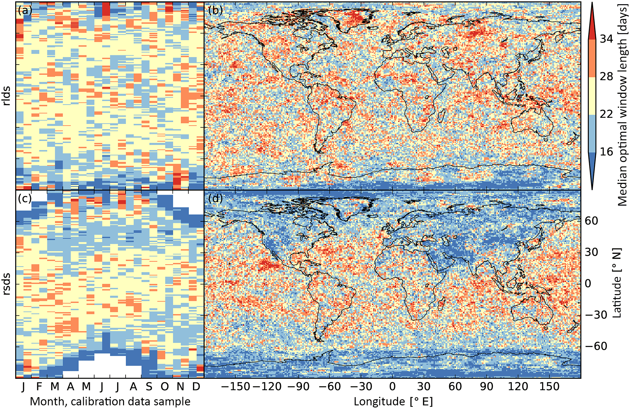
Figure D1Optimal window length for running mean and maximum calculations that precede the estimation of parameters of the climatological distributions of longwave (v=l; top) and shortwave (v=s; bottom) radiation that are used for bias correction with BCvda1 (see Table 1). Window lengths are varied between 10 and 40 days. Optimal window lengths maximise the p value of the two-sample KS statistic of bias-corrected E2OBS data cross validated against SRB data (see Sect. 4 and Appendix C) and are determined individually for every grid cell, calendar month (with all corresponding values pooled into one distribution), and calibration data sample (every1st, every2nd). Zonal medians of optimal window lengths for each month and calibration data sample are shown in panels (a) and (c). Results are masked in (c) where and when the monthly mean rsdt (Eqs. B1–B4) is less than 1 W m−2. Panels (b) and (d) show medians of optimal window lengths over months and calibration data samples.
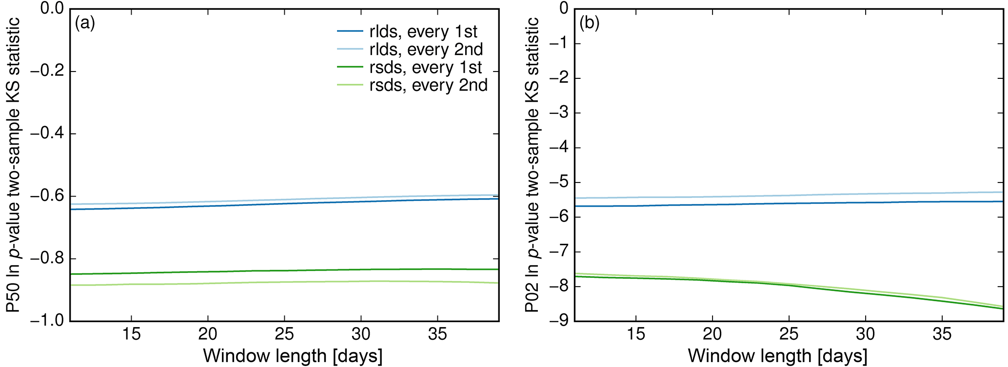
Figure D2Dependence of two-sample KS statistic p values on window length for different radiation types and calibration data samples (see text and Fig. D1). Plotted are the grid-cell area-weighted 50th (a) and second (b) percentiles of the natural logarithms of the p values over months, latitudes, and longitudes.
The author declares that no competing interests are present.
The author is grateful to Katja Frieler, Jan Volkholz, and Alex Cannon for
various helpful discussions at different stages of this work, to Paul
W. Stackhouse Jr. for his guidance with SRB data products and the provision
of SRB elevation data, to Graham Weedon and Emanuel Dutra for their guidance
during the initial stage of assembling the EWEMBI dataset, and to the two
anonymous referees, who provided highly valuable comments on the discussion
paper version of this paper. This work has received funding from the
European Union's Horizon 2020 research and innovation programme under grant
agreement no. 641816 Coordinated Research in Earth Systems and Climate:
Experiments, kNowledge, Dissemination and Outreach
(CRESCENDO).
The article processing charges
for this open-access
publication were covered by the Potsdam
Institute
for Climate Impact Research (PIK).
Edited by:
Valerio Lucarini
Reviewed by: two anonymous referees
Calton, B., Schellekens, J., and Martinez-de la Torre, A.: Water Resource Reanalysis v1: Data Access and Model Verification Results, https://doi.org/10.5281/zenodo.57760, 2016. a, b, c
Cannon, A. J.: Multivariate quantile mapping bias correction: an N-dimensional probability density function transform for climate model simulations of multiple variables, Clim. Dynam., 50, 1–19, https://doi.org/10.1007/s00382-017-3580-6, 2017. a
Chang, J., Ciais, P., Wang, X., Piao, S., Asrar, G., Betts, R., Chevallier, F., Dury, M., François, L., Frieler, K., Ros, A. G. C., Henrot, A.-J., Hickler, T., Ito, A., Morfopoulos, C., Munhoven, G., Nishina, K., Ostberg, S., Pan, S., Peng, S., Rafique, R., Reyer, C., Rödenbeck, C., Schaphoff, S., Steinkamp, J., Tian, H., Viovy, N., Yang, J., Zeng, N., and Zhao, F.: Benchmarking carbon fluxes of the ISIMIP2a biome models, Environ. Res. Lett., 12, 045002, https://doi.org/10.1088/1748-9326/aa63fa, 2017. a
Dee, D. P., Uppala, S. M., Simmons, A. J., Berrisford, P., Poli, P., Kobayashi, S., Andrae, U., Balmaseda, M. A., Balsamo, G., Bauer, P., Bechtold, P., Beljaars, A. C. M., van de Berg, L., Bidlot, J., Bormann, N., Delsol, C., Dragani, R., Fuentes, M., Geer, A. J., Haimberger, L., Healy, S. B., Hersbach, H., Hólm, E. V., Isaksen, L., Kållberg, P., Köhler, M., Matricardi, M., McNally, A. P., Monge-Sanz, B. M., Morcrette, J.-J., Park, B.-K., Peubey, C., de Rosnay, P., Tavolato, C., Thépaut, J.-N., and Vitart, F.: The ERA-Interim reanalysis: configuration and performance of the data assimilation system, Q. J. Roy. Meteor. Soc., 137, 553–597, https://doi.org/10.1002/qj.828, 2011. a, b
Dutra, E.: Report on the current state-of-the-art Water Resources Reanalysis, Earth2observe deliverable no. d.5.1, available at: http://earth2observe.eu/files/Public Deliverables (last access: 18 May 2018), 2015. a, b
Fisher, R. A.: Frequency Distribution of the Values of the Correlation Coefficient in Samples from an Indefinitely Large Population, Biometrika, 10, 507–521, 1915. a
Fisher, R. A.: On the “probable error” of a coefficient of correlation deduced from a small sample, Metron., 1, 3–32, 1921. a
Frieler, K., Lange, S., Piontek, F., Reyer, C. P. O., Schewe, J., Warszawski, L., Zhao, F., Chini, L., Denvil, S., Emanuel, K., Geiger, T., Halladay, K., Hurtt, G., Mengel, M., Murakami, D., Ostberg, S., Popp, A., Riva, R., Stevanovic, M., Suzuki, T., Volkholz, J., Burke, E., Ciais, P., Ebi, K., Eddy, T. D., Elliott, J., Galbraith, E., Gosling, S. N., Hattermann, F., Hickler, T., Hinkel, J., Hof, C., Huber, V., Jägermeyr, J., Krysanova, V., Marcé, R., Müller Schmied, H., Mouratiadou, I., Pierson, D., Tittensor, D. P., Vautard, R., van Vliet, M., Biber, M. F., Betts, R. A., Bodirsky, B. L., Deryng, D., Frolking, S., Jones, C. D., Lotze, H. K., Lotze-Campen, H., Sahajpal, R., Thonicke, K., Tian, H., and Yamagata, Y.: Assessing the impacts of 1.5 ∘C global warming – simulation protocol of the Inter-Sectoral Impact Model Intercomparison Project (ISIMIP2b), Geosci. Model Dev., 10, 4321–4345, https://doi.org/10.5194/gmd-10-4321-2017, 2017. a
Garratt, J. R.: Incoming Shortwave Fluxes at the Surface – A Comparison of GCM Results with Observations, J. Climate, 7, 72–80, https://doi.org/10.1175/1520-0442(1994)007<0072:ISFATS>2.0.CO;2, 1994. a
Gennaretti, F., Sangelantoni, L., and Grenier, P.: Toward daily climate scenarios for Canadian Arctic coastal zones with more realistic temperature-precipitation interdependence, J. Geophys. Res.-Atmos., 120, 11862–11877, https://doi.org/10.1002/2015JD023890, 2015. a
Gudmundsson, L., Bremnes, J. B., Haugen, J. E., and Engen-Skaugen, T.: Technical Note: Downscaling RCM precipitation to the station scale using statistical transformations – a comparison of methods, Hydrol. Earth Syst. Sci., 16, 3383–3390, https://doi.org/10.5194/hess-16-3383-2012, 2012. a, b
Harris, I., Jones, P. D., Osborn, T. J., and Lister, D. H.: Updated high-resolution grids of monthly climatic observations – the CRU TS3.10 Dataset, Int. J. Climatol., https://doi.org/10.1002/joc.3711, 2013. a
Hempel, S., Frieler, K., Warszawski, L., Schewe, J., and Piontek, F.: A trend-preserving bias correction – the ISI-MIP approach, Earth Syst. Dynam., 4, 219-236, https://doi.org/10.5194/esd-4-219-2013, 2013. a
Iizumi, T., Takikawa, H., Hirabayashi, Y., Hanasaki, N., and Nishimori, M.: Contributions of different bias-correction methods and reference meteorological forcing data sets to uncertainty in projected temperature and precipitation extremes, J. Geophys. Res.-Atmos., 122, 2017JD026613, https://doi.org/10.1002/2017JD026613, 2017. a
Ito, A., Nishina, K., Reyer, C. P. O., François, L., Henrot, A.-J., Munhoven, G., Jacquemin, I., Tian, H., Yang, J., Pan, S., Morfopoulos, C., Betts, R., Hickler, T., Steinkamp, J., Ostberg, S., Schaphoff, S., Ciais, P., Chang, J., Rafique, R., Zeng, N., and Zhao, F.: Photosynthetic productivity and its efficiencies in ISIMIP2a biome models: benchmarking for impact assessment studies, Environ. Res. Lett., 12, 085001, https://doi.org/10.1088/1748-9326/aa7a19, 2017. a
Jones, P. W.: First- and Second-Order Conservative Remapping Schemes for Grids in Spherical Coordinates, Mon. Weather Rev., 127, 2204–2210, https://doi.org/10.1175/1520-0493(1999)127<2204:FASOCR>2.0.CO;2, 1999. a
Kalnay, E., Kanamitsu, M., Kistler, R., Collins, W., Deaven, D., Gandin, L., Iredell, M., Saha, S., White, G., Woollen, J., Zhu, Y., Leetmaa, A., Reynolds, R., Chelliah, M., Ebisuzaki, W., Higgins, W., Janowiak, J., Mo, K. C., Ropelewski, C., Wang, J., Jenne, R., and Joseph, D.: The NCEP/NCAR 40-Year Reanalysis Project, B. Am. Meteorol. Soc., 77, 437–471, https://doi.org/10.1175/1520-0477(1996)077<0437:TNYRP>2.0.CO;2, 1996. a, b
Kiehl, J. T. and Trenberth, K. E.: Earth's Annual Global Mean Energy Budget, B. Am. Meteorol. Soc., 78, 197–208, https://doi.org/10.1175/1520-0477(1997)078<0197:EAGMEB>2.0.CO;2, 1997. a
Kistler, R., Collins, W., Saha, S., White, G., Woollen, J., Kalnay, E., Chelliah, M., Ebisuzaki, W., Kanamitsu, M., Kousky, V., van den Dool, H., Jenne, R., and Fiorino, M.: The NCEP-NCAR 50-Year Reanalysis: Monthly Means CD-ROM and Documentation, B. Am. Meteorol. Soc., 82, 247–267, https://doi.org/10.1175/1520-0477(2001)082<0247:TNNYRM>2.3.CO;2, 2001. a
Kolmogorov, A.: Sulla determinazione empirica di una leggi di distribuzione, Giornale dell' Istituto Italiano degli Attuari, 4, 83–91, 1933. a
Kopp, G. and Lean, J. L.: A new, lower value of total solar irradiance: Evidence and climate significance, Geophys. Res. Lett., 38, l01706, https://doi.org/10.1029/2010GL045777, 2011. a
Krysanova, V. and Hattermann, F. F.: Intercomparison of climate change impacts in 12 large river basins: overview of methods and summary of results, Climatic Change, 141, 363–379, https://doi.org/10.1007/s10584-017-1919-y, 2017. a
Kuiper, N. H.: Tests concerning random points on a circle, in: Koninklijke Nederlandse Akademie van Wetenschappen, vol. 63 of A, 38–47, 1962. a
Lange, S.: EartH2Observe, WFDEI and ERA-Interim data Merged and Bias-corrected for ISIMIP (EWEMBI), https://doi.org/10.5880/pik.2016.004, 2016. a, b
Ma, Q., Wang, K., and Wild, M.: Evaluations of atmospheric downward longwave radiation from 44 coupled general circulation models of CMIP5, J. Geophys. Res.-Atmos., 119, 4486–4497, https://doi.org/10.1002/2013JD021427, , 2014. a
Maraun, D.: Bias Correction, Quantile Mapping, and Downscaling: Revisiting the Inflation Issue, J. Climate, 26, 2137–2143, https://doi.org/10.1175/JCLI-D-12-00821.1, 2013. a, b
Müller Schmied, H., Müller, R., Sanchez-Lorenzo, A., Ahrens, B., and Wild, M.: Evaluation of Radiation Components in a Global Freshwater Model with Station-Based Observations, Water, 8, 450, https://doi.org/10.3390/w8100450, 2016. a
Ruane, A. C., Goldberg, R., and Chryssanthacopoulos, J.: Climate forcing datasets for agricultural modeling: Merged products for gap-filling and historical climate series estimation, Agr. Forest Meteorol., 200, 233–248, https://doi.org/10.1016/j.agrformet.2014.09.016, 2015. a, b, c, d, e, f, g, h
Rust, H. W., Kruschke, T., Dobler, A., Fischer, M., and Ulbrich, U.: Discontinuous Daily Temperatures in the WATCH Forcing Datasets, J. Hydrometeorol., 16, 465–472, https://doi.org/10.1175/JHM-D-14-0123.1, 2015. a
Sheffield, J., Goteti, G., and Wood, E. F.: Development of a 50-Year High-Resolution Global Dataset of Meteorological Forcings for Land Surface Modeling, J. Climate, 19, 3088–3111, https://doi.org/10.1175/JCLI3790.1, 2006. a, b, c, d
Smirnov, N.: Table for Estimating the Goodness of Fit of Empirical Distributions, Ann. Math. Stat., 19, 279–281, https://doi.org/10.1214/aoms/1177730256, 1948. a
Stackhouse Jr., P. W., Gupta, S. K., Cox, S. J., Mikovitz, C., Zhang, T., and Hinkelman, L. M.: The NASA/GEWEX surface radiation budget release 3.0: 24.5-year dataset, Gewex news, 21, 10–12, 2011. a, b, c
Stephens, M. A.: The Goodness-Of-Fit Statistic Vn: Distribution and Significance Points, Biometrika, 52, 309–321, https://doi.org/10.2307/2333685, 1965. a
Stephens, M. A.: Use of the Kolmogorov-Smirnov, Cramer-Von Mises and Related Statistics Without Extensive Tables, J. R. Stat. Soc. Series B. Met., 32, 115–122, 1970. a
Switanek, M. B., Troch, P. A., Castro, C. L., Leuprecht, A., Chang, H.-I., Mukherjee, R., and Demaria, E. M. C.: Scaled distribution mapping: a bias correction method that preserves raw climate model projected changes, Hydrol. Earth Syst. Sci., 21, 2649–2666, https://doi.org/10.5194/hess-21-2649-2017, 2017. a
Trenberth, K. E., Fasullo, J. T., and Kiehl, J.: Earth's Global Energy Budget, B. Am. Meteorol. Soc., 90, 311–323, https://doi.org/10.1175/2008BAMS2634.1, 2009. a
Uppala, S. M., Kållberg, P. W., Simmons, A. J., Andrae, U., Bechtold, V. D. C., Fiorino, M., Gibson, J. K., Haseler, J., Hernandez, A., Kelly, G. A., Li, X., Onogi, K., Saarinen, S., Sokka, N., Allan, R. P., Andersson, E., Arpe, K., Balmaseda, M. A., Beljaars, A. C. M., Berg, L. V. D., Bidlot, J., Bormann, N., Caires, S., Chevallier, F., Dethof, A., Dragosavac, M., Fisher, M., Fuentes, M., Hagemann, S., Hólm, E., Hoskins, B. J., Isaksen, L., Janssen, P. A. E. M., Jenne, R., Mcnally, A. P., Mahfouf, J.-F., Morcrette, J.-J., Rayner, N. A., Saunders, R. W., Simon, P., Sterl, A., Trenberth, K. E., Untch, A., Vasiljevic, D., Viterbo, P., and Woollen, J.: The ERA-40 re-analysis, Q. J. Roy. Meteor. Soc., 131, 2961–3012, https://doi.org/10.1256/qj.04.176, 2005. a
Veldkamp, T. I. E., Wada, Y., Aerts, J. C. J. H., Döll, P., Gosling, S. N., Liu, J., Masaki, Y., Oki, T., Ostberg, S., Pokhrel, Y., Satoh, Y., Kim, H., and Ward, P. J.: Water scarcity hotspots travel downstream due to human interventions in the 20th and 21st century, Nat. Commun., 8, 15697, https://doi.org/10.1038/ncomms15697, 2017. a
Vetterling, W. T., Press, W. H., Teukolsky, S. A., and Flannery, B. P.: Numerical Recipes in C (The Art of Scientific Computing), Cambridge University Press, 2nd edn., 620–628, 1992. a, b
Weedon, G. P., Gomes, S., Viterbo, P., Österle, H., Adam, J. C., Bellouin, N., Boucher, O., and Best, M.: The WATCH forcing data 1958–2001: A meteorological forcing dataset for land surface and hydrological models, Technical report no. 22, available at: http://www.eu-watch.org/publications/technical-reports (last access: 18 May 2018), 2010. a
Weedon, G. P., Gomes, S., Viterbo, P., Shuttleworth, W. J., Blyth, E., Österle, H., Adam, J. C., Bellouin, N., Boucher, O., and Best, M.: Creation of the WATCH Forcing Data and Its Use to Assess Global and Regional Reference Crop Evaporation over Land during the Twentieth Century, J. Hydrometeorol., 12, 823–848, https://doi.org/10.1175/2011JHM1369.1, 2011. a, b, c
Weedon, G. P., Balsamo, G., Bellouin, N., Gomes, S., Best, M. J., and Viterbo, P.: The WFDEI meteorological forcing data set: WATCH Forcing Data methodology applied to ERA-Interim reanalysis data, Water Resour. Res., 50, 7505–7514, https://doi.org/10.1002/2014WR015638, 2014. a, b, c
Wild, M., Folini, D., Schär, C., Loeb, N., Dutton, E. G., and König-Langlo, G.: The global energy balance from a surface perspective, Clim. Dynam., 40, 3107–3134, https://doi.org/10.1007/s00382-012-1569-8, 2013. a
Wild, M., Folini, D., Hakuba, M. Z., Schär, C., Seneviratne, S. I., Kato, S., Rutan, D. A., Ammann, C., Wood, E. F., and König-Langlo, G.: The energy balance over land and oceans: an assessment based on direct observations and CMIP5 climate models, Clim. Dynam., 44, 3393–3429, https://doi.org/10.1007/s00382-014-2430-z, 2015. a
Wilks, D. S.: Statistical Methods in the Atmospheric Sciences, Academic Press, San Diego, CA, 1995. a, b
Xu, X.: Methods in Hypothesis Testing, Markov Chain Monte Carlo and Neuroimaging Data Analysis, PhD thesis, Harvard University, available at: http://nrs.harvard.edu/urn-3:HUL.InstRepos:11108711 (last access: 18 May 2018), 2013. a
Zhao, M. and Dirmeyer, P. A.: Production and analysis of GSWP-2 near-surface meteorology data sets, Center for Ocean-Land-Atmosphere Studies Calverton, available at: http://ww.w.monsoondata.org/gswp/gswp2data.pdf (last access: 18 May 2018), 2003. a
- Abstract
- Introduction
- Data
- Methods
- Results
- Summary and conclusions
- Data availability
- Appendix A: Quantile mapping and statistical downscaling
- Appendix B: Daily mean insolation at the top of the atmosphere
- Appendix C: Two-sample Kolmogorov–Smirnov test and Kuiper's two-sample test
- Appendix D: Window length for running mean and maximum calculations
- Competing interests
- Acknowledgements
- References