the Creative Commons Attribution 4.0 License.
the Creative Commons Attribution 4.0 License.
 | 18 Apr 2018
Quantifying changes in spatial patterns of surface air temperature dynamics over several decades
Dario A. Zappalà
Marcelo Barreiro
Cristina Masoller
We study daily surface air temperature (SAT) reanalysis in a grid over the Earth's surface to identify and quantify changes in SAT dynamics during the period 1979–2016. By analysing the Hilbert amplitude and frequency we identify the regions where relative variations are most pronounced (larger than ±50 % for the amplitude and ±100 % for the frequency). Amplitude variations are interpreted as due to changes in precipitation or ice melting, while frequency variations are interpreted as due to a northward shift of the inter-tropical convergence zone (ITCZ) and to a widening of the rainfall band in the western Pacific Ocean. The ITCZ is the ascending branch of the Hadley cell, and thus by affecting the tropical atmospheric circulation, ITCZ migration has far-reaching climatic consequences. As the methodology proposed here can be applied to many other geophysical time series, our work will stimulate new research that will advance the understanding of climate change impacts.
- Article
(2949 KB) - Full-text XML
-
Supplement
(5659 KB) - BibTeX
- EndNote


The unprecedented intensification of weather extremes is motivating research aimed at understanding long-term climatic variations (Barreiro et al., 2008; Cai et al., 2014; Coumou and Rahmstorf, 2012; England et al., 2014; Turco et al., 2015) that can have profound socio-economic impacts (Ghil et al., 2011) and trigger complex ecological adaptation mechanisms (Beaumont et al., 2011; Bordeu et al., 2016; Gottfried et al., 2012; Lejeune et al., 2002).
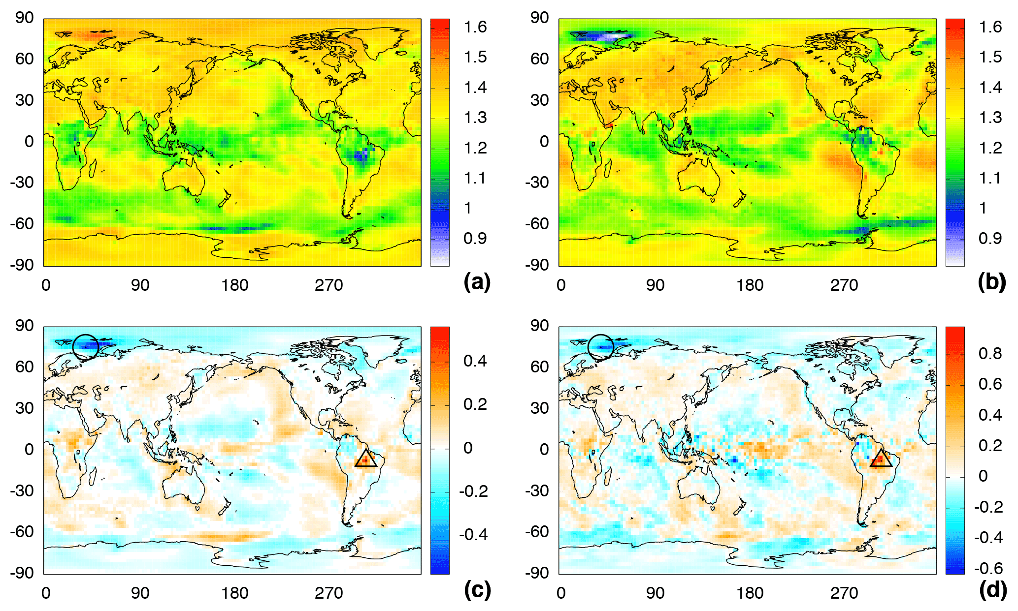
Figure 1Relative change in the time-averaged Hilbert amplitude. (a) Amplitude averaged over the first 10 years (January 1979 to December 1988). (b) Amplitude averaged over the last 10 years (July 2007 to June 2016). (c) Relative change in the Hilbert amplitude, . (d) Relative change in amplitude of the seasonal cycle computed from the amplitude of the climatology, Δa(clim)∕a(clim). A good qualitative agreement is seen in the spatial structures in (c) and (d). Importantly, the structures uncovered by the Hilbert amplitude are well defined in comparison with those uncovered by the analysis of the climatology amplitude, which look noisier.
Quantifying variations in surface air temperature (SAT) dynamics over several decades is a challenging problem because of non-stationarity and the presence of trends, measurement noise, multiple timescales, memory, and correlations in the data (Franzke, 2012; Massah and Kantz, 2016); in addition, reanalysis data can be unreliable (due to the lack of observational constraints in many geographical regions), and reanalysis time series are insufficiently long (as reanalysis starts at the beginning of the satellite era). These challenges have motivated the use, for climate data analysis, of data-driven approaches that have been commonly used for investigating observed complex signals in other fields of science (e.g. neurological, physiological, financial, etc.). Univariate analysis tools that have been used to analyse SAT time series include detrended fluctuation analysis, fractional analysis, and wavelet analysis. Bivariate analysis and the complex network approach has also allowed us to uncover inter-relations between SAT anomalies in different regions (Barreiro et al., 2011; Donges et al., 2009; Tsonis and Swanson, 2008). In this approach the seasonal cycle is removed to eliminate the influence of solar forcing, and the links represent correlations (linear or non-linear) or statistical similarities between SAT dynamics in different areas (Tirabassi and Masoller, 2016). On the other hand, changes in the SAT seasonal cycle have also been investigated, and a trend toward reduced cycle amplitude has been detected in many regions (Chambers et al., 2013; Duan et al., 2017; Dwyer et al., 2012; Qian et al., 2011; Stine and Huybers, 2012; Stine et al., 2009; Wang and Dillon, 2014). However, changes in SAT dynamics over several decades (such as those observed in Fig. 1) have not yet been investigated at a global scale. In order to fill this gap, we use Hilbert analysis (described in the Supplement) to investigate SAT time series with daily resolution (reanalysis covering the Earth's surface in the period 1979–2016). Our goal is to detect the most sensitive regions (“hotspots”) where variations in SAT dynamics over the last decades are more pronounced.
The Hilbert transform (HT) provides, for a real oscillatory time series, x(t) with t ∈ [1, T], an instantaneous amplitude, a(t), and an instantaneous frequency, ω(t), for each data point of the time series and thus allows us to characterise how the amplitude and the frequency of a signal vary in time. If a signal does not have a sufficiently narrow frequency band, a(t) and ω(t) will not have a clear physical meaning (Pikovsky et al., 2001). The usual solution is based on band-pass filtering to isolate a narrow frequency band; however, HT directly applied to the signal can still yield useful information. An alternative solution is based on the Hilbert–Huang transform (Huang et al., 1998) that combines Hilbert analysis with empirical mode decomposition that decomposes an arbitrary real time series into components, each having the physical meaning of a rotation in the complex plane.
Because many natural geophysical time series have a seasonal periodicity, this has motivated the use of Hilbert analysis to characterise the time-varying oscillation amplitude and to investigate phase shifts and phase–amplitude couplings. Applications in various geophysical fields are discussed in Huang and Wu (2008). As more recent examples, Massei and Fournier (2012) used Hilbert analysis to characterise the daily variability of the Seine river flow from 1950 to 2008, uncovering linkages between river flow variability and global climate oscillations (the North Atlantic Oscillation and the Madden–Julian Oscillation). Sun (2015) used Hilbert analysis to compute the daily phase shift between temperature signals recorded at the ground surface and at a depth of 5 m in two meteorology stations in Taiwan from 1952 to 2008. Significant reductions in the phase shift from the 1980s to 1990s were found, which was interpreted to be related to the warming of the Pacific Decadal Oscillation. Reddy and Adarsh (2016) applied Hilbert analysis to rainfall time series in India and found that the multi-scale components of rainfall series have a similar periodic structure as global climate oscillations (the Quasi-biennial Oscillation, El Niño Southern Oscillation, etc.).
We have recently applied the Hilbert transform to unfiltered daily SAT reanalysis (Zappalà et al., 2016). We have shown that the maps of time-averaged Hilbert frequency, , and standard deviation, σω, revealed well-defined large-scale structures which were consistent with known dynamical processes.
Here we use a(t) and ω(t) to quantify SAT variations. Our hypothesis is that changes in a(t) and ω(t) can yield information about variations in SAT dynamics. Specifically, we are interested in addressing the following questions: which properties of a(t) and ω(t) display relevant variations? Where are the regions in which these variations are more pronounced? Which processes can be responsible for these variations? Can these variations be used as a quantitative measure of regional climate change?
In the main text we present results from an ERA-Interim daily SAT reanalysis (Dee et al., 2011) that covers the period from January 1979 to June 2016 with a spatial resolution of 2.5∘, both in latitude and in longitude. Thus, there are N = 73 × 144 = 10 512 geographical sites and in each site the SAT time series has T=13696 days. In the Supplement we compare ERA-Interim with NCEP-DOE Reanalysis 2, which is an improved version of the NCEP Reanalysis I model (Kistler et al., 2001). It covers a longer time interval and has 94 × 192 = 18 048 geographical sites. In order to perform a precise comparison between the results of the two datasets, in the NCEP-DOE Reanalysis 2 we consider the same time interval as the ERA-Interim dataset.
3.1 Hilbert analysis
To apply the Hilbert transform (described in the Supplement) we first pre-process each raw SAT time series, rj(t) (where j ∈ [1, N] represents the geographical site and t ∈ [1, T] represents the day): we eliminate the linear trend and normalise to zero mean and unit variance, obtaining xj(t). The Hilbert transform is then applied to xj(t), obtaining yj(t) = HT[xj(t)]. From xj(t) and yj(t), the amplitude aj(t) and the phase φj(t) were calculated as aj(t) = and φj(t) = arctan[yj(t)∕xj(t)]. Taking into account the signs of xj(t) and yj(t), the phase is constrained to the interval [−π, π). Whenever an extreme value of the interval is reached, the phase jumps to the other end of the interval. By eliminating these sudden jumps (using a standard library function that appropriately adds ±2π) we “unwrapped” the phase obtaining a continuous variation in time from which the frequency time series, ωj(t), was obtained by calculating the derivative. Since the Hilbert algorithm (Bilato et al., 2014) gives deviations from the true values of the amplitude, phase, and frequency near the extremes, in each time series (aj(t), φj(t), and ωj(t)) we disregarded the initial and final 5% (see the Supplement). This way, we have time series of length T = 12 328.
3.2 Measures used to quantify variations in SAT dynamics
Variations in the Hilbert amplitude were quantified by the relative change, = ( − , where is the average value of the amplitude during the first 10 years of the time series (January 1979 to December 1988), and during the last 10 years (July 2007 to June 2016). Analogously, we calculated the relative change in amplitude variance, , of average frequency, , and of frequency variance, . In the Supplement we analyse how the spatial structures uncovered depend on the time intervals used to calculate the relative variations: we compare with relative variations during the first and final 5 years of the reanalysis and also during the first half-period and the second half-period of the reanalysis. While the values of the relative variations vary with the time interval considered, the spatial maps are remarkably robust as the same structures are found with the three time intervals considered.
A similar analysis was performed to detect changes directly from the raw SAT time series, rj(t), by computing the amplitude of the climatology (or seasonal cycle), cj(t), and the variance of anomaly time series, zj(t).
Specifically, the amplitude of the climatology was calculated as = max[] − min[], where is the climatology series calculated only in the time interval I. We remark that the climatology amplitude is a scalar number that depends on the choice of the time interval I. We calculated the climatology amplitude in the first and last decade, as well as in the whole series. As before, we used these values to calculate the relative change Δa(clim)∕a(clim). Also, the variance of the anomaly time series zj(t) was calculated and then used to find the relative change, .
With the goal of relating changes in Hilbert frequency with changes in the statistical properties of SAT time series, an analysis of the number of zero crossings was performed: for each xj(t) we counted the number of crossings through the mean value, x = 0. As with other quantities, we then calculated the relative change.
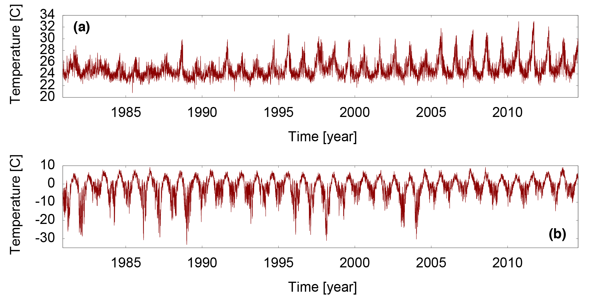
Figure 2Surface air temperature in two regions where a clear change in the oscillation amplitude in the last 10 years is observed with respect to the first 10 years. (a) Site of coordinates (7.5∘ S, 307.5∘ E) marked with a triangle in Fig. 1c. (b) Site of coordinates (75∘ N, 40∘ E) marked with a circle in Fig. 1c.
3.3 Significance analysis
A statistical significance analysis was performed by surrogating Hilbert series. For each amplitude time series (i.e. in each grid point) 100 shuffle surrogates were generated and for each surrogate the relative change, , was calculated. Then, the average over the 100 surrogates, , and its standard deviation, σs, were used to define the significance threshold: the relative change computed from the original data was considered significant if it was higher than + 2σs or lower than − 2σs. In the colour maps, regions where variations are not significant are displayed in white. The same test was applied to frequency variations and the other quantities, except for the climatology for which a surrogate test is not applicable. In the Supplement various thresholds are considered and, in addition, a non-parametric significance test is used. Here we present only the maps obtained with threshold ±2σ because it is a compromise between uncovering the spatial regions where SAT changes are pronounced and disregarding the areas where the variations are small.
We analyse the maps of , , , and in the first 10 years and in the last 10 years of the period covered by the reanalysis, as well as the relative change between the two decades.
4.1 Analysis of amplitude variations
Figure 1a and b display in the first and in the last 10 years, respectively, and Fig. 1c displays the relative difference (see Sect. 3 for details). In Fig. 1c we see an area of large increase (more than 50 %) in average amplitude located in South America (red spot marked by a triangle) and an area of large decrease (again, more than 50 %) located in the Arctic (blue spot marked by a circle). The raw SAT time series in these regions are displayed in Fig. 2.
In both time series we clearly observe a change in the amplitude of the oscillations in the last 10 years with respect to the first 10 years, having a visual confirmation of the changes detected by the Hilbert amplitude. The red spot in Amazonia, whose SAT series shown in Fig. 2a has an increasing amplitude, can be interpreted in terms of changes in precipitation. In particular, the increase in the Hilbert amplitude is linked to the decrease in precipitation and to the lengthening of the dry season (as reported in Fu et al., 2013; Gu et al., 2016; Liebmann et al., 2004). This is due to the fact that when precipitation decreases, the fraction of solar radiation that is not used for evaporation is used to heat the ground, which in turn heats the surface air. This leads to higher extreme temperatures during the dry seasons, as can be observed in Fig. 2a. Regarding the blue spot in the Arctic region where the SAT series shown in Fig. 2b has a decreasing amplitude, it can be interpreted as due to the melting of sea ice. In fact, when ice is present at the surface of the sea, it acts as an insulator preventing heat exchange between sea and air. This causes a large amplitude in the SAT cycle. On the other hand, if the ice melts, the air–sea heat exchange reduces the amplitude of the cycle. In particular, during winter the air temperature is mitigated by the sea and tends to have more moderated values. It is important to take into account that this blue spot is in a region for which the observational constraints from satellites on the reanalysis are scarce, which decreases the quality of the reanalysis in the region. Therefore, in order to check whether the detected changes are robust, we performed the same analysis using the NCEP-DOE reanalysis dataset. The results, presented in the Supplement, confirm the presence of the blue spot in the Arctic.
Next, we compare the changes detected by the Hilbert amplitude with those computed directly from SAT (by decomposing the SAT time series into climatology and anomaly, as explained in Sect. 3). Since the climatology term retains the seasonal variation, we expect its amplitude change to give similar indications as the Hilbert amplitude change. On the other hand, the anomaly term contains all the rapid variability, so we expect its variance to give similar results as the variance of the Hilbert amplitude.
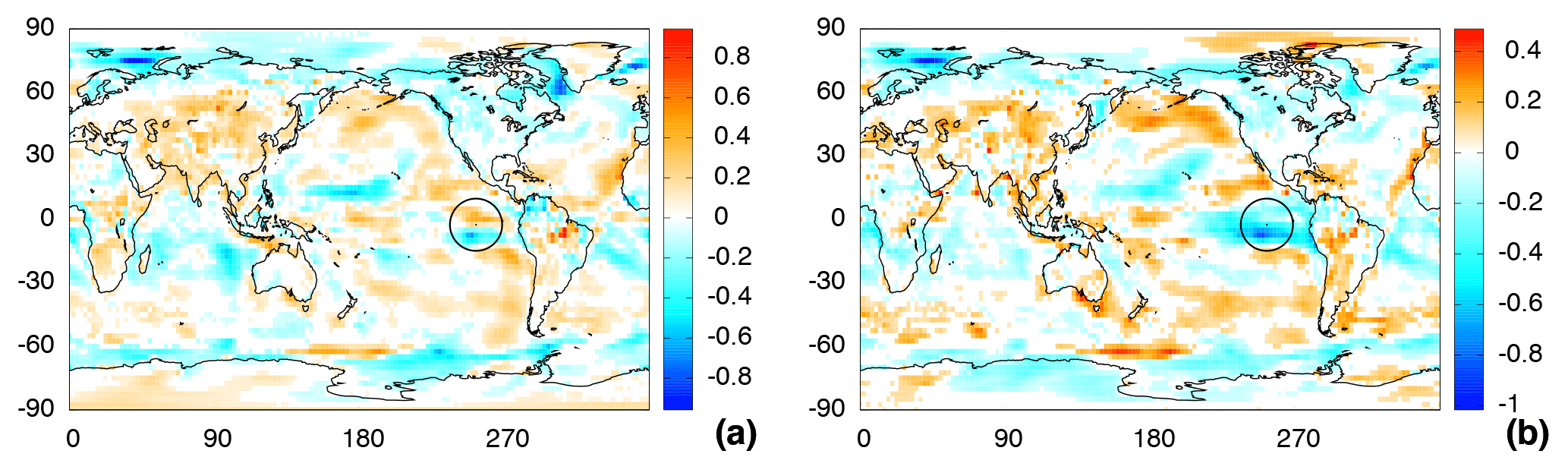
Figure 3Relative change in amplitude fluctuations computed from the variance of the (a) Hilbert amplitude, ; (b) the anomaly time series, .

Figure 4Relative change in the time-averaged Hilbert frequency (in units of oscillations per year). (a) Average in the first 10 years (1979–1988). (b) Average in the last 10 years (2007–2016). (c) Relative change in Hilbert frequency, . (d) Relative change in the number of zero crossings of the normalised SAT time series. In (a) and (b) the colour scale is adjusted to represent in white the regions where the average frequency is one oscillation per year. In (c) and (d), a good qualitative agreement of spatial structures is seen; however, we note that the Hilbert frequency detects stronger variations than those measured by the number of zero crossings.
Figure 1c and d, which respectively display the relative change in Hilbert amplitude and in climatology amplitude, and Fig. 3a and b, which respectively display the relative change in Hilbert amplitude variance and in anomaly variance, confirm these expectations.
The good qualitative agreement seen in the spatial structures in these maps confirms that Hilbert analysis directly applied to unfiltered SAT indeed gives a physically meaningful instantaneous amplitude, with average and variance values that are consistent with those computed from SAT.
In Fig. 3a and b, however, there is a difference in the eastern Pacific Ocean in the area marked with a circle. In particular, in Fig. 3b there is an area with large decrease in variance (dark blue, around −100 %), while in Fig. 3a the decrease is less pronounced (light blue, around −65 %) and extended over a smaller area. In addition, in Fig. 3a there is a reddish orange area that indicates a moderate increase in variance (around 45 %), while in Fig. 3b such an area is absent. The reasons underlying these differences will be discussed later.
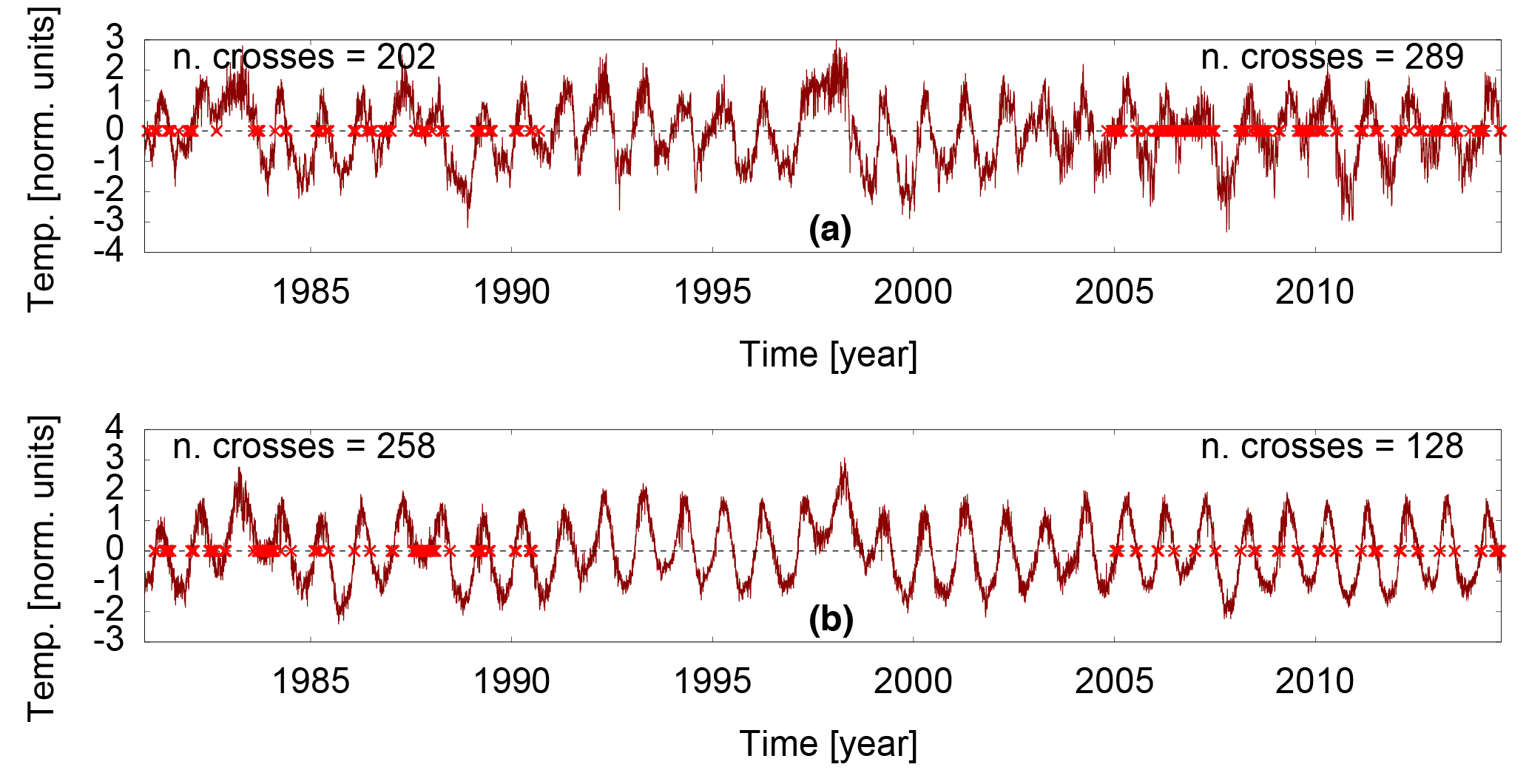
Figure 5Normalised SAT time series and number of zero crossings in the regions indicated with a circle in Fig. 4c. In the red region (2.5∘ N, 245∘ E) (a), the number of zero crossings increases in the last 10 years with respect to the first 10 years (289 and 202, respectively), while in the blue region (7.5∘ S, 250∘ E) (b), it decreases (128 and 258 in the last and first 10 years).
4.2 Analysis of frequency variations
Figure 4a displays the average frequency in the first 10 years, Fig. 4b in the last 10 years, and Fig. 4c displays the relative change, . In Fig. 4c we note that in the eastern Pacific Ocean there are two small areas, enclosed by the circle, of intense increase (red) and decrease (blue) in frequency. They both represent frequency changes whose absolute values are larger than 100 % and correspond to the same region where differences were detected in Fig. 3.
These two areas of opposite signs suggest that, between the initial and the final decade, there is a shift of the inter-tropical convergence zone (ITCZ) toward the north. The ITCZ involves strong convective activity, which causes rapid fluctuations of SAT, thus giving high values of instantaneous frequency, as shown in Fig. 4a and b. Therefore, in the relative change in frequency, in regions corresponding to the initial position of the ITCZ we see a decrease, while in regions corresponding to the present position of the ITCZ we see an increase. For the same reason, the two red areas in the western Pacific Ocean (indicated by two squares) suggest an expansion of the tropical convective regions. This interpretation is in agreement with previous works that have related a northward shift of the ITCZ to an inter-hemispheric temperature gradient, such as the one experienced during the last decades (Frierson and Hwang, 2012; Kang et al., 2009; Schneider et al., 2014; Talento and Barreiro, 2016; Yoshimori and Broccoli, 2008). Regarding the red areas in the north Atlantic, the north Pacific, and the south Pacific, they are consistent with an increase in the occurrence of fronts, which cause large daily fluctuations of temperature and thus an increase in the Hilbert frequency.
To gain insight into the physical meaning of the changes that are captured by the Hilbert frequency, we use an alternative approach to estimate frequency variations: we define “events” as the zero crossings of SAT time series (Pikovsky et al., 2001) (detrended and normalised to zero mean as described in Sect. 3). Then, we count the number of events in the first 10 years and in the last 10 years and calculate the relative variation.
Figure 4d displays the map of relative change in zero crossings. We see that there is a qualitative good agreement with the spatial structures seen in Fig. 4c, thus providing a physical interpretation for the observed variation in the Hilbert frequency: the areas where the frequency increases (decreases) correspond to areas where the number of zero crossings increases (decreases). We note that the relative variations in the Hilbert frequency are more pronounced than those in the number of crossings, and this specifically holds in the regions where frequency variations are interpreted in terms of ITCZ migration.
Figure 5a and b display SAT time series in the dipole region indicated with the circle in Fig. 4c and also indicate (in red) the zero crossings. We can understand the difference that was detected in this region between the variance of the Hilbert amplitude (Fig. 3a) and the variance of the anomaly (Fig. 3b). This difference is explained in the following terms: in the first decade the seasonal cycle is more irregular than in the last decade, probably a consequence of an El Niño event in 1982–1983. The anomaly series contains these slow fluctuations as well as the rapid ones, and thus its variance is affected by both effects. In contrast, the Hilbert amplitude is less affected by the slow fluctuations as its variance captures mainly the rapid fluctuations of SAT.
To demonstrate the robustness of our findings, in the Supplement we compare the results obtained from ERA-Interim with those obtained from another reanalysis dataset, NCEP-DOE. We find a good qualitative agreement in the spatial structures in the maps of , , , and , but we also discuss some relevant differences. In addition, to further understand the relationship between the statistical properties of SAT and those of the Hilbert amplitude and frequency, in the Supplement we apply Hilbert analysis to synthetic data generated by an autoregressive AR(1) process. We chose an AR(1) process because it is commonly used in the literature to model climate data. We find that, when increasing the noise intensity in the synthetic series, the Hilbert amplitude decreases while the frequency increases, which shows that this trend is also observed in real SAT time series.
We have used Hilbert analysis to quantify the changes in SAT dynamics, on a global scale, that have occurred over the last 3 decades. From the SAT time series with daily resolution we derived the amplitude and the frequency time series and then calculated the relative change (between the first and the last decade) in the average and variance of these series. Large variations in the Hilbert amplitude (more than 50 %) in the Arctic and in Amazonia were respectively interpreted as due to ice melting and precipitation decrease. The analysis of the Hilbert frequency also uncovered areas of large changes. In particular, two areas of opposite changes in the eastern Pacific Ocean and two areas of increase in the western Pacific Ocean suggest a shift towards the north and a widening of the ITCZ. While there is evidence that the ITCZ has moved north–south in the past, to the best of our knowledge our work is the first to confirm this migration in the last decades. Our findings have important implications because, as the ITCZ is the ascending branch of the Hadley cell, its migration affects both the Earth's radiative balance and the release of latent heat that drives the tropical atmospheric circulation. Taken together, these effects have not only local but also far-reaching climatic consequences. Additional analysis provided in the Supplement confirms the robustness of these observations.
As the methodology used here can be applied to many other climatological time series that exhibit well-defined oscillatory behaviour, we believe that our work will stimulate new research to identify and quantify the impacts of climate change directly from observed data.
The Hilbert algorithm used is available in Bilato et al. (2014); the datasets used are the ERA-Interim Reanalysis provided by the European Centre For Medium-Range Weather Forecasts (ECMWF), Reading, UK, from their website (https://www.ecmwf.int, Dee et al., 2011) and the NCEP-DOE Reanalysis 2 provided by NOAA, Boulder, Colorado, USA, from their website (http://www.esrl.noaa.gov/psd/, Kanamitsu et al., 2002).
The supplement related to this article is available online at: https://doi.org/10.5194/esd-9-383-2018-supplement.
The authors declare that they have no conflict of interest.
This work was supported in part by the LINC project (EU-FP7-289447), ICREA
ACADEMIA (Generalitat de Catalunya, Spain), and by the Spanish MINECO/FEDER
(FIS2015-66503-C3-2-P). Dario A. Zappalà also thanks the European Social Fund and
the Generalitat de Catalunya for the FI-AGAUR scholarship.
Edited by: Sagnik Dey
Reviewed by: two anonymous referees
Barreiro, M., Fedorov, A., Pacanowski, R., and Philander, S. G.: Abrupt climate changes: How freshening of the northern Atlantic affects the thermohaline and wind-driven oceanic circulations, Annu. Rev. Earth Planet. Sci., 36, 33–58, 2008. a
Barreiro, M., Marti, A. C., and Masoller, C.: Inferring long memory processes in the climate network via ordinal pattern analysis, Chaos, 21, 013101, https://doi.org/10.1063/1.3545273, 2011. a
Beaumont, L. J., Pitman, A., Perkins, S., Zimmermann, N. E., Yoccoz, N. G., and Thuiller, W.: Impacts of climate change on the world's most exceptional ecoregions, P. Natl. Acad. Sci. USA, 108, 2306–2311, 2011. a
Bilato, R., Maj, O., and Brambilla, M.: An algorithm for fast Hilbert transform of real functions, Adv. Comput. Math., 40, 1159–1168, https://doi.org/10.1007/s10444-014-9345-4, 2014. a, b
Bordeu, I., Clerc, M. G., Couteron, P., Lefever, R., and Tlidi, M.: Self-replication of localized vegetation patches in scarce environments, Sci. Rep., 6, 33703, https://doi.org/10.1038/srep33703, 2016. a
Cai, W., Borlace, S., Lengaigne, M., van Rensch, P., Collins, M., Vecchi, G., Timmermann, A., Santoso, A., McPhaden, M. J., Wu, L., England, M. H., Wang, G., Guilyardi, E., and Jin, F.-F.: Increasing frequency of extreme El Niño events due to greenhouse warming, Nat. Clim. Change, 4, 111–116, 2014. a
Chambers, L. E., Altwegg, R., Barbraud, C., Barnard, P., Beaumont, L. J., Crawford, R. J. M., Durant, J. M., Hughes, L., Keatley, M. R., Low, M., Morellato, P. C., Poloczanska, E. S., Ruoppolo, V., Vanstreels, R. E. T., Woehler, E. J., and Wolfaardt, A. C.: Phenological changes in the southern hemisphere, PLoS ONE, 8, e75514, https://doi.org/10.1371/journal.pone.0075514, 2013. a
Coumou, D. and Rahmstorf, S.: A decade of weather extremes, Nat. Clim. Change, 2, 491–496, 2012. a
Dee, D. P., Uppala, S. M., Simmons, A. J., Berrisford, P., Poli, P., Kobayashi, S., Andrae, U., Balmaseda, M. A., Balsamo, G., Bauer, P., Bechtold, P., Beljaars, A. C. M., van de Berg, L., Bidlot, J., Bormann, N., Delsol, C., Dragani, R., Fuentes, M., Geer, A. J., Haimberger, L., Healy, S. B., Hersbach, H., Hólm, E. V., Isaksen, L., Kållberg, P., Köhler, M., Matricardi, M., McNally, A. P., Monge-Sanz, B. M., Morcrette, J.-J., Park, B.-K., Peubey, C., de Rosnay, P., Tavolato, C., Thépaut, J.-N., and Vitart, F.: The ERA-Interim reanalysis: configuration and performance of the data assimilation system, Q. J. Roy. Meteorol. Soc., 137, 553–597, https://doi.org/10.1002/qj.8282011, 2011. a, b
Donges, J. F., Zou, Y., Marwan, N., and Kurths, J.: The backbone of the climate network, Europhys. Lett., 87, 48007, https://doi.org/10.1209/0295-5075/87/48007, 2009. a
Duan, J., Esper, J., Büntgen, U., Li, L., Xoplaki, E., Zhang, H., Wang, L., Fang, Y., and Luterbacher, J.: Weakening of annual temperature cycle over the tibetan plateau since the 1870s, Nat. Comm., 8, 14008, https://doi.org/10.1038/ncomms14008, 2017. a
Dwyer, J., Biasutti, M., and Sobel, A.: Projected changes in the seasonal cycle of surface temperature, J. Climate, 25, 6359–6374, 2012. a
England, M. H., McGregor, S., Spence, P., Meehl, G. A., Timmermann, A., Cai, W., Gupta, A. S., McPhaden, M. J., Purich, A., and Santoso, A.: Recent intensification of wind-driven circulation in the pacific and the ongoing warming hiatus, Nat. Clim. Change, 4, 222–227, 2014. a
Franzke, C.: Nonlinear trends, long-range dependence, and climate noise properties of surface temperature, J. Climate, 25, 4172–4183, 2012. a
Frierson, D. M. W., and Hwang, Y. T.: Extratropical influence on ITCZ shifts in slab ocean simulations of global warming, J. Climate, 25, 720–733, 2012. a
Fu, R., Yin, L., Li, W., Arias, P. A., Dickinson, R. E., Huang, L., Chakraborty, S., Fernandes, K., Liebmann, B., Fisher, R., and Myneni, R. B.: Increased dry-season length over southern amazonia in recent decades and its implication for future climate projection, P. Natl. Acad. Sci. USA, 110, 18110–18115, 2013. a
Ghil, M., Yiou, P., Hallegatte, S., Malamud, B. D., Naveau, P., Soloviev, A., Friederichs, P., Keilis-Borok, V., Kondrashov, D., Kossobokov, V., Mestre, O., Nicolis, C., Rust, H. W., Shebalin, P., Vrac, M., Witt, A., and Zaliapin, I.: Extreme events: dynamics, statistics and prediction, Nonlin. Processes Geophys., 18, 295–350, https://doi.org/10.5194/npg-18-295-2011, 2011. a
Gottfried, M., Pauli, H., Futschik, A., Akhalkatsi, M., Barančok, P., Alonso, J. L. B., Coldea, G., Dick, J., Erschbamer, B., Fernández Calzado, M. R., Kazakis, G., Krajči, J., Larsson, P., Mallaun, M., Michelsen, O., Moiseev, D., Moiseev, P., Molau, U., Merzouki, A., Nagy, L., Nakhutsrishvili, G., Pedersen, B., Pelino, G., Puscas, M., Rossi, G., Stanisci, A., Theurillat, J.-P., Tomaselli, M., Villar, L., Vittoz, P., Vogiatzakis, I., and Grabherr, G.: Continent-wide response of mountain vegetation to climate change, Nat. Clim. Change, 2, 111–115, 2012. a
Gu, G., Adler, R. F., and Huffman, G. J.: Long-term changes/trends in surface temperature and precipitation during the satellite era (1979–2012), Clim. Dynam., 46, 1091–1105, 2016. a
Huang, N. E., Shen, Z., Long, S. R., Wu, M. C., Shih, H. H., Zheng, Q., Yen, N.-C., Tung, C. C., and Liu, H. H.: The empirical mode decomposition and the Hilbert spectrum for nonlinear and non-stationary time series analysis, P. Roy. Soc. Lond. A, 454, 903–995, 1998. a
Huang, N. E., and Wu, Z.: A review on Hilbert-Huang transform: Method and its applications to geophysical studies, Rev. Geophys., 46, 8755–1209, 2008. a
Kanamitsu, M., Ebisuzaki, W., Woollen, J., Yang, S.-K., Hnilo, J. J., Fiorino, M., and Potter, G. L.: NCEP-DOE AMIP-II Reanalysis (R-2), B. Am. Meteorol. Soc., 83, 1631–1643, https://doi.org/10.1175/BAMS-83-11-1631, 2002. a
Kang, S. M., Frierson, D. M. W., and Held, I.: The tropical response to extratropical thermal forcing in an idealized GCM: The importance of radiative feedbacks and convective parameterization, J. Atmos. Sci., 66, 2812–2827, 2009. a
Kistler, R., Kalnay, E., Collins, W., Saha, S., White, G., Woollen, J., Chelliah, M., Ebisuzaki, W., Kanamitsu, M., Kousky, V., van den Dool, H., Jenne, R., and Fiorino, M.: The NCEP-NCAR 50-year reanalysis: Monthly means CD-ROM and documentation, B. Am. Meteorol. Soc., 82, 247–268, 2001. a
Lejeune, O., Tlidi, M., and Couteron, P.: Localized vegetation patches: A self-organized response to resource scarcity, Phys. Rev. E, 66, 010901, https://doi.org/10.1103/PhysRevE.66.010901, 2002. a
Liebmann, B., Vera, C. S., Carvalho, L. M. V., Camilloni, I. A., Hoerling, M. P., Allured, D., Barros, V. R., Báez, J., and Bidegain, M.: An observed trend in central south american precipitation, J. Climate, 17, 4357–4367, 2004. a
Massah, M. and Kantz, H.: Confidence intervals for time averages in the presence of long-range correlations, a case study on earth surface temperature anomalies, Geophys. Res. Lett., 43, 9243–9249, 2016. a
Massei, N. and Fournier, M.: Assessing the expression of large-scale climatic fluctuations in the hydrological variability of daily seine river flow (France) between 1950 and 2008 using Hilbert–Huang transform, J. Hydrol., 448, 119–128, 2012. a
Pikovsky, A., Rosenblum, M., and Kurths, J.: Synchronization: A universal concept in nonlinear sciences, Cambridge University Press, Cambridge, 2001. a, b
Qian, C., Fu, C., and Wu, Z.: Changes in the amplitude of the temperature annual cycle in china and their implication for climate change research, J. Climate, 24, 5292–5302, 2011. a
Reddy, M. J. and Adarsh, S.: Time-frequency characterization of sub-divisional scale seasonal rainfall in India using the Hilbert–Huang transform, Stoch. Environ. Res. Risk A., 30, 1063–1085, 2016. a
Schneider, T., Bischoff, T., and Haug, G. H.: Migrations and dynamics of the intertropical convergence zone, Nature, 513, 45–53, 2014. a
Stine, A. and Huybers, P.: Changes in the seasonal cycle of temperature and atmospheric circulation, J. Climate, 25, 7362–7380, 2012. a
Stine, A. R., Huybers, P., and Fung, I. Y.: Changes in the phase of the annual cycle of surface temperature, Nature, 457, 435–440, 2009. a
Sun, Y.-Y.: Instantaneous phase shift of annual subsurface temperature cycles derived by the Hilbert-Huang transform, J. Geophys. Res.-Atmos., 120, 1670–1677, 2015. a
Talento, S. and Barreiro, M.: Simulated sensitivity of the tropical climate to extratropical thermal forcing: tropical SSTs and African land surface, Clim. Dynam., 47, 1091–1110, 2016. a
Tirabassi, G. and Masoller, C.: Unravelling the community structure of the climate system by using lags and symbolic time-series analysis, Sci. Rep., 6, 29804, https://doi.org/10.1038/srep29804, 2016. a
Tsonis, A. and Swanson, K.: Topology and predictability of El Niño and La Niña networks, Phys. Rev. Lett., 100, 228502, https://doi.org/10.1103/PhysRevLett.100.228502, 2008. a
Turco, M., Palazzi, E., von Hardenberg, J., and Provenzale, A.: Observed climate change hotspots, Geophys. Res. Lett., 42, 3521–3528, 2015. a
Wang, G. and Dillon, M.: Recent geographic convergence in diurnal and annual temperature cycling flattens global thermal profiles, Nat. Clim. Change, 4, 988–992, 2014. a
Yoshimori, M. and Broccoli, A. J.: Equilibrium response of an atmosphere-mixed layer ocean model to different radiative forcing agents: Global and zonal mean response, J. Climate, 21, 4399–4423, 2008. a
Zappalà, D. A., Barreiro, M., and Masoller, C.: Global atmospheric dynamics investigated by using Hilbert frequency analysis, Entropy, 18, 408, 2016. a