the Creative Commons Attribution 4.0 License.
the Creative Commons Attribution 4.0 License.
 | 13 Mar 2018
Regional scaling of annual mean precipitation and water availability with global temperature change
Lukas Gudmundsson
Sonia I. Seneviratne
Changes in regional water availability belong to the most crucial potential impacts of anthropogenic climate change, but are highly uncertain. It is thus of key importance for stakeholders to assess the possible implications of different global temperature thresholds on these quantities. Using a subset of climate model simulations from the fifth phase of the Coupled Model Intercomparison Project (CMIP5), we derive here the sensitivity of regional changes in precipitation and in precipitation minus evapotranspiration to global temperature changes. The simulations span the full range of available emission scenarios, and the sensitivities are derived using a modified pattern scaling approach. The applied approach assumes linear relationships on global temperature changes while thoroughly addressing associated uncertainties via resampling methods. This allows us to assess the full distribution of the simulations in a probabilistic sense. Northern high-latitude regions display robust responses towards wetting, while subtropical regions display a tendency towards drying but with a large range of responses. Even though both internal variability and the scenario choice play an important role in the overall spread of the simulations, the uncertainty stemming from the climate model choice usually accounts for about half of the total uncertainty in most regions. We additionally assess the implications of limiting global mean temperature warming to values below (i) 2 K or (ii) 1.5 K (as stated within the 2015 Paris Agreement). We show that opting for the 1.5 K target might just slightly influence the mean response, but could substantially reduce the risk of experiencing extreme changes in regional water availability.
- Article
(14788 KB) - Full-text XML
-
Supplement
(6212 KB) - BibTeX
- EndNote


Assessing regional changes in mean-annual precipitation, P, and precipitation minus evapotranspiration, P − E (often also referred to as water availability), in the context of on-going global warming is of high relevance for a wide range of socio-economic sectors. Regional differences in P and P − E pose important challenges to farmers, water resources managers, stakeholders and decision-makers and a comprehensive, easily accessible communication and visualization of complex climate model output is necessary to allow for targeted adaptation and mitigation strategies.
The public and political debate on climate change is usually limited to a debate about global temperature change, which is, however, an abstract measure and does not enable end-users to infer direct implications for regional to local climate change, especially also with respect to hydroclimatological variables (Seneviratne et al., 2016; Victor and Kennel, 2014). However, due to its omnipresence in popular climate communication, global mean temperature T could be used as a general measure of climate change and thereby enable a different communication of regional climate impacts to the public: “The regional change of a climate variable as a function of global warming”. Many studies use approaches following this guideline, with one of the most common techniques used being summarized as “pattern scaling”.
In this study, we follow the tradition of pattern scaling but introduce a more rigorous, probabilistic assessment of the underlying uncertainties. Common pattern scaling approaches originally have the goal to use a spatial response pattern in a certain variable (e.g. regional temperature, precipitation) that is derived from observational or (usually) from climate model data with respect to global mean temperature or CO2 changes in order to create a large number of additional scenarios (Mitchell, 2003; Santer et al., 1990). In this study, we use the “large number of additional scenarios” created by the utilized pattern scaling technique to estimate the uncertainty distribution of the response pattern in a probabilistic approach. Pattern scaling approaches have been employed in a large number of studies (see, e.g. Tebaldi and Arblaster, 2014 for an overview), but many common approaches to estimate the response pattern are also subject to an ongoing debate (Herger et al., 2015; Kravitz et al., 2017; Tebaldi and Arblaster, 2014). To estimate the spatial response pattern in mean-annual P and P − E, we adapt here a technique based on the assumption that the scaling relationship between local temperature at each grid point and global mean temperature is linear and that the resulting maps of regression slopes could be used as the response pattern (Solomon et al., 2009). Following a more empirical approach without a priori assumptions on the relationship of regional variables to global temperature, it was recently shown that these findings also hold for extreme temperatures and extreme precipitation, mostly independent of emission scenarios (Seneviratne et al., 2016). This approach was further applied and extended in Wartenburger et al. (2017) by using a comprehensive set of hydroclimatological variables, including both mean-annual P and P − E. The assessment presented in this work builds upon the analysis presented in Wartenburger et al. (2017) by utilizing a similar data collection to quantify the associated response pattern.
The scaling relationship between global mean P and global warming has also been analysed in previous studies (Andrews et al., 2009; Fischer et al., 2014; Frieler et al., 2011; Pendergrass and Hartmann, 2012; Pendergrass et al., 2015). At global scales, mean precipitation scales positively with global temperature increase (Knutti et al., 2016), but the associated scaling coefficient is still subject to an ongoing debate and might not necessarily follow a linear relationship (Good et al., 2016). It was further shown that the magnitude of the scaling relationship depends on the emission scenario (Andrews et al., 2009; Frieler et al., 2011; Pendergrass and Hartmann, 2012; Pendergrass et al., 2015), whereas the scaling relationship of extreme precipitation is independent of the emission scenario (Pendergrass et al., 2015; Seneviratne et al., 2016). The scaling relationship between global mean P − E and global warming was, to our knowledge, only assessed in Wartenburger et al. (2017), and more research is needed to evaluate the full range of potential impacts of regional water availability change.
We aim here to develop a methodological framework in order to assess regional changes in mean-annual P and P − E over global land areas with respect to global warming by using a representative subset of climate models and considering different emission scenarios. We further account for the internal variability of each projection by considering the year-to-year variability of P and P − E. This enables us to generate conservative estimates of the uncertainty distribution of the scaling coefficient for P and P − E at every grid point and within specific regions.
Another issue addressed within this study is related to the implications of different global warming-degree targets on regional P and P − E. At the United Nations Climate Change Conference held in Paris in 2015 (COP21), most nations agreed to limit the increase in global mean temperature to values “well below 2 K” and to ideally not surpass a warming of 1.5 K above pre-industrial conditions. Thereby, previous goals to limit global warming to “only” 2 K global warming are significantly intensified. However, this raises the question of potential implications and differences between these “warming-degree targets” with respect to changes in many other climate variables besides the (rather abstract) value of global mean temperature and especially at regional scales (Guiot and Cramer, 2016; James et al., 2017; Schleussner et al., 2016; Seneviratne et al., 2016). The framework developed within this study allows us to directly assess regional changes in P and P − E in the context of these warming-degree targets, thereby providing important and useful information to decision-makers, farmers, water resources managers, stakeholders and the general public within a specific region.
First, we introduce the climate model data that are utilized within this study before describing the methodological approach that is used to estimate the uncertainty distribution of the scaling coefficients of P and P − E with respect to global warming (Sect. 2). We provide in the following illustrations of the median and the range of the scaling coefficients (Sect. 3). Next, we comprehensively assess the uncertainty that is stemming from the choice of emission scenario (Sect. 3.1) and how other sources of uncertainty contribute to the total uncertainty (Sect. 3.2). We further apply the new framework to analyse changes between different warming-degree targets (Sect. 4) and summarize and discuss our results also within the context of previous assessments (Sect. 5).
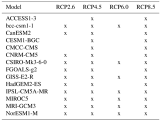
The fifth phase of the Coupled Model Intercomparison Project (CMIP5) ensemble (Taylor et al., 2012) includes climate model projections forced by four Representative Concentration Pathway (RCP) emission scenarios (Moss et al., 2010). These scenarios correspond to their relative radiative forcings reached by the end of the 21st century with respect to the pre-industrial period: 2.6, 4.5, 6.0 and 8.5 W m−2 (from here on referred to as RCP2.6, RCP4.5, RCP6.0 and RCP8.5). We use a total of 14 climate models selected based on prerequisites provided in Fischer et al. (2014), which are only one model from each modelling centre and thereof the newest with the highest resolution. Please note that not all climate models provide data for all emission scenarios (see Table 1). We consider a time period of 120 years beginning in 1980 and ending in 2099 comprising historical simulations for the first 26 years which emerge into simulations of the respective emission scenarios from 2006 onwards. The first 20 years (1980–1999) are used as a common baseline period, and values in mean-annual P and P − E are assessed in relative terms (%) with respect to the baseline period. Since we focus here on global land areas, please note that in the case of P − E < 0 for all models and scenarios, those grid points were neglected.
For each model m and each emission scenario s within the 100-year period (2000–2099), the relative values of precipitation, , and precipitation minus evapotranspiration, (P − , are regressed at each grid point (or averaged over a certain region) against mean-annual global temperature, ). We use an ordinary least squares fit to estimate the parameters of the linear equation,
with rm,s denoting the regression slope and Im,s the intercept (and likewise for (P − ). The slope itself provides us with an estimate of the regional scaling coefficient of P against global changes in T.
Given the annual residuals = − , the uncertainty of the regression slope rm,s is assessed by resampling years yr′ of the residuals () and fitting the regression slope against the new pairs (, + ). Repeating this approach 1000 times at each grid point (or within each specific region) provides us with a comprehensive uncertainty measure ϵm,s of each model- and scenario-specific regression slope rm,s for both P and P − E. We like to point out that the uncertainty estimated through resampling residuals results in very similar results as computing the uncertainty through using different realizations of a single model (this is shown for CSIRO-Mk3-6-0 in Fig. S1 in the Supplement). We further note that scaling coefficients in low-latitude regions represent the response within a larger area compared to those in high-latitude regions. To also test the validity of the linearity assumption, we assessed (i) if the Kolmogorov–Smirnov test does not reject the null hypothesis that the annual residuals are normally distributed and (ii) if there is no significant lag – 1-year autocorrelation of all (please see Fig. S2). Following this approach, in the majority of world regions and for most models, the linearity assumption is potentially valid. However, please note, for the following sections, that in many hyper-arid regions both tests fail for the majority of models. Hence, a linear scaling approach might not be the most appropriate method to assess sensitivities in these regions and potentially causes spurious results.
Table 1List of models and availability under each emission scenario.
This approach allows us to distinguish between three different sources of uncertainty. As illustrated in the conceptual Fig. 1, these are (i) internal variability, σi, representing the uncertainty stemming from interannual variability for each model under each scenario; (ii) the model uncertainty, σm, related to the uncertainty across all models and for a specific scenario (e.g. in terms of variance: σm = − μr)2, with n = 14 models and μr denoting the average of all scaling coefficient); and (iii) the scenario uncertainty, σs, related to the uncertainty across all scenarios and for a specific model or the multimodel mean (e.g. in terms of variance: σs = − μr)2, with n = 4 scenarios and μr denoting the average of all scaling coefficients). The total uncertainty denotes the uncertainty across all models, all scenarios and considering the internal uncertainty. Please note that this approach of attributing uncertainties is very simplistic and neglects any potential relationship between the individual sources of uncertainty, but is suitable and useful to provide a general measure of the underlying uncertainty sources.
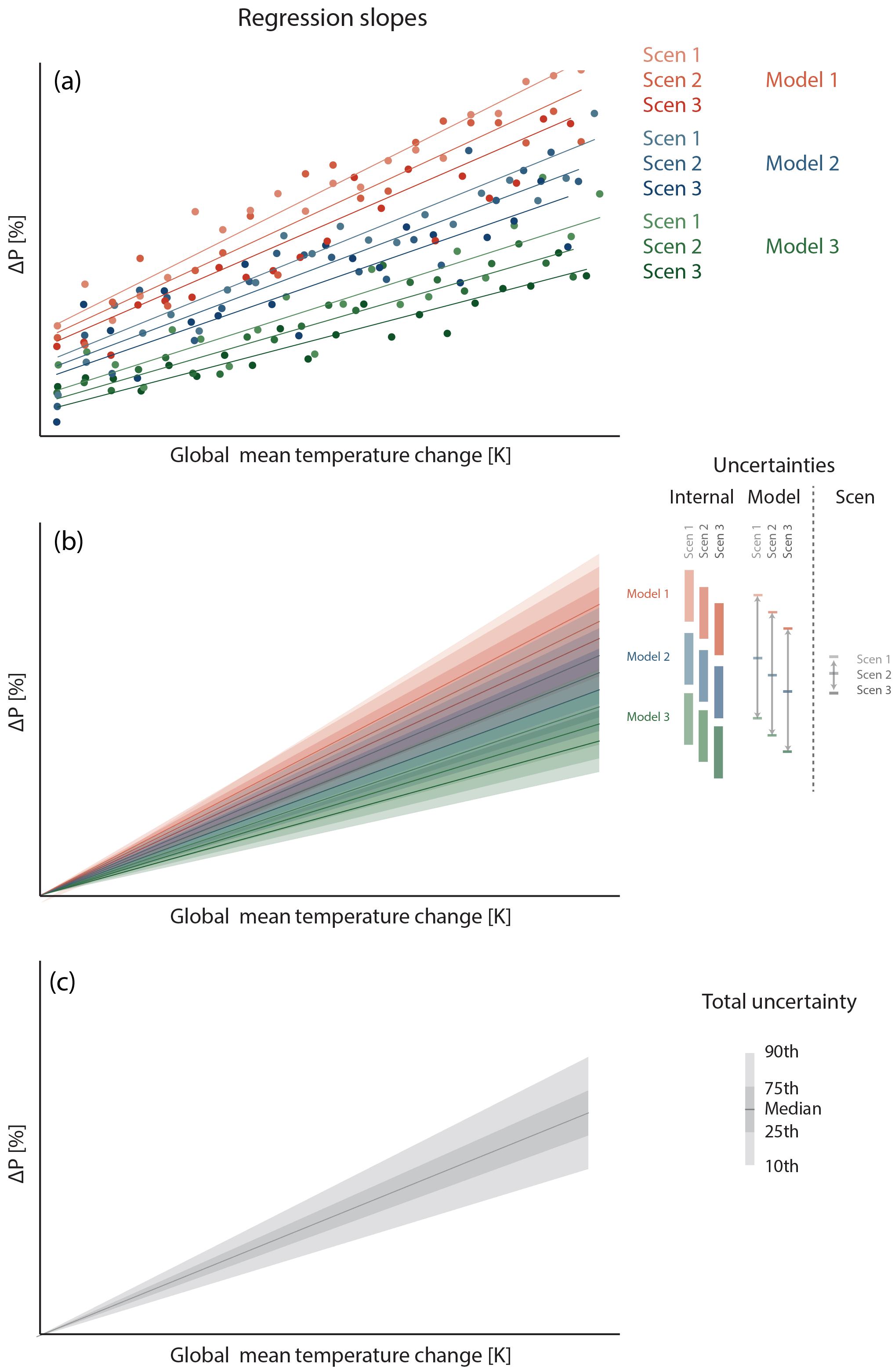
Figure 1Conceptual illustration of deriving the uncertainty distribution of the scaling coefficient of P with respect to global warming from multiple models forced by multiple emission scenarios. (a) For each model under each scenario, we regress the relative change in mean-annual P (ΔP, with respect to a baseline period) against global mean T. We thereby obtain the regression slope which is the scaling coefficient of P to global warming. The year-to-year variability further causes the estimate of the slope to be uncertain. We account for this uncertainty by numerically estimating the uncertainty distribution of each model- and scenario-specific regression slope through resampling the residuals in a bootstrapping approach. (b) This uncertainty is associated with every model run and represents the internal variability. The average of the uncertainties stemming from the range of all individual models within a certain scenario represents the model uncertainty, and the uncertainty associated with the range of all scenario-specific multimodel means represents the scenario uncertainty. The uncertainty distribution is illustrated here as a function of global temperature increase. (c) The total uncertainty combines all sources of uncertainty and provides a conservative estimate of regional ΔP as a function of global warming that can be used to assess either the median response or to study changes in any other quantile of the uncertainty distribution.
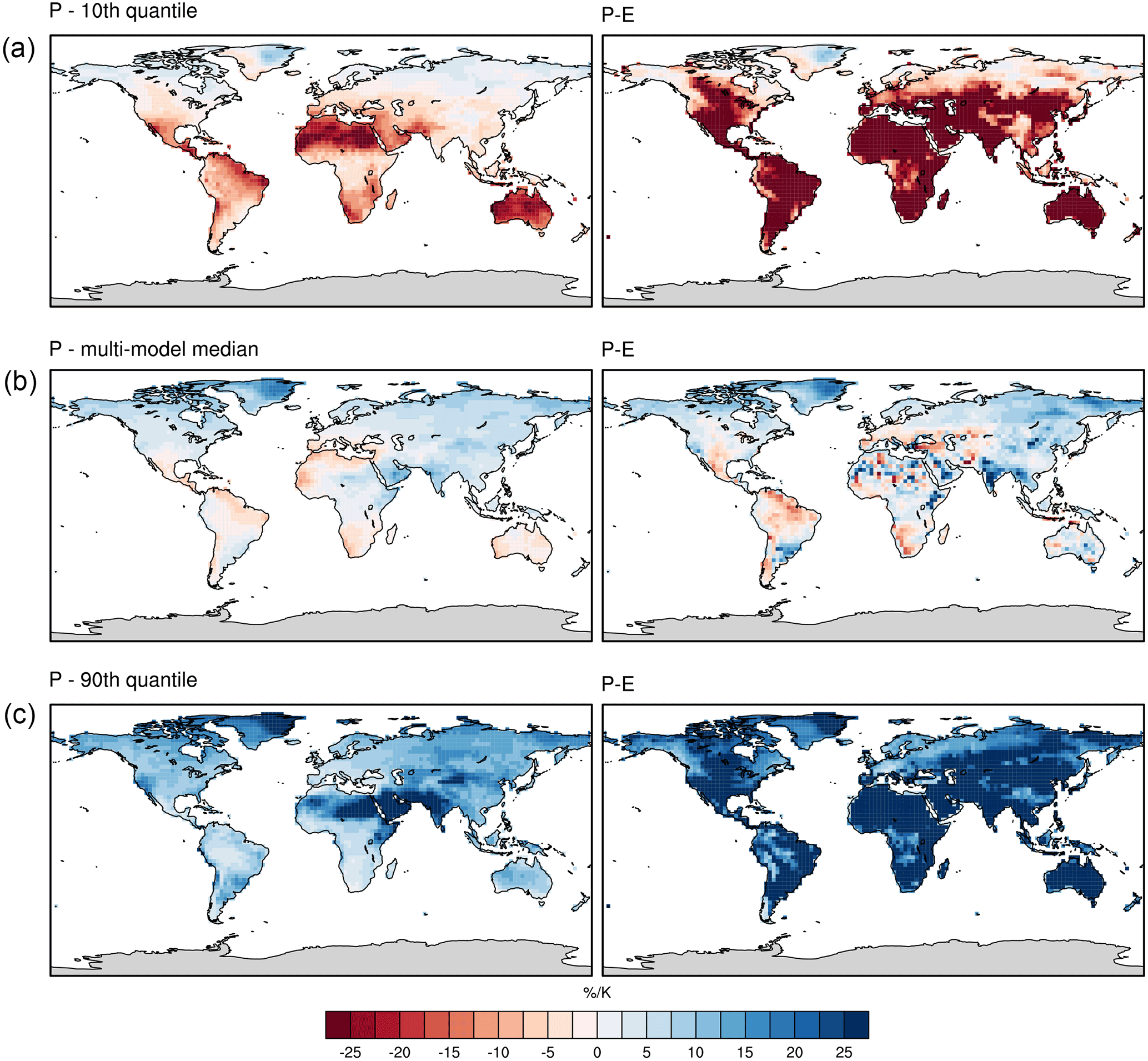
Figure 2Median (b), 10th (a) and 90th quantiles (c) of the sensitivity of P (left panels) and P − E (right panels) to changes in global mean temperature (% K−1). A total of 14 CMIP5 models and all scenarios (RCP2.6, RCP4.5, RCP6.0, RCP8.5) are considered.
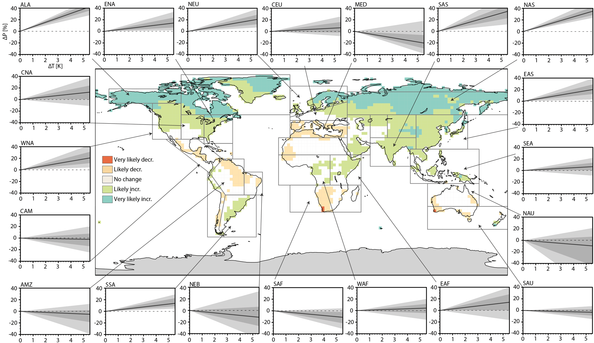
Figure 3Conceptual summary of the probability that the slope of P is negatively/positively different from zero considering all climate models and all scenarios. Panel plots illustrates the uncertainty distribution of the sensitivity of P to global temperature change as a function of global mean temperature change averaged for each SREX (Special Report on Managing the Risks of Extreme Events and Disasters to Advance Climate Change Adaptation) region outlined in the map (the shading in each panel plot corresponds to those illustrated in Fig. 1).
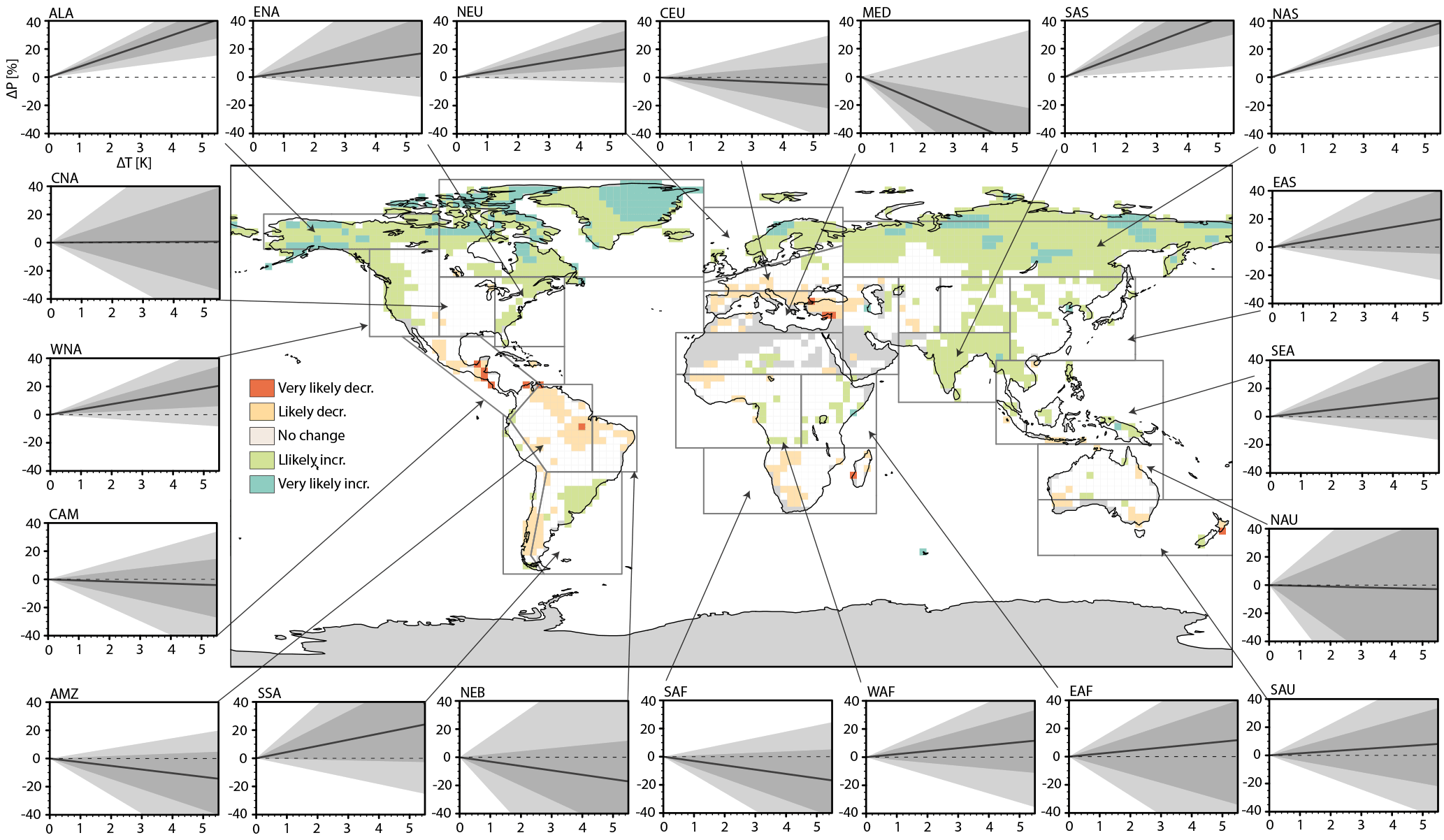
Figure 4Conceptual summary of the probability that the slope of P − E is negatively/positively different from zero considering all climate models and all scenarios. Panel plots show the uncertainty distribution of the sensitivity of P − E to global temperature change as a function of global mean temperature change averaged for each SREX region outlined in the map (the shading in each panel plot corresponds to those illustrated in Fig. 1).
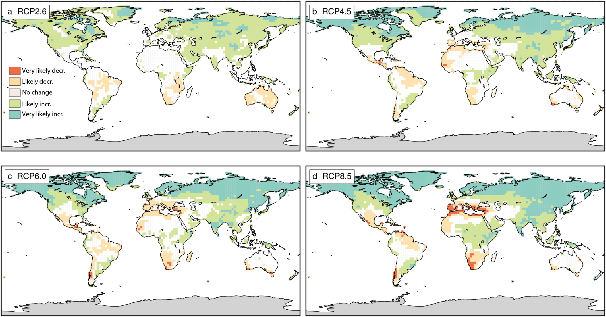
Figure 5Conceptual summary of the probability that the slope of P is negatively/positively different from zero considering all climate models and (a) the RCP2.6, (b) the RCP4.5, (c) RCP6.0 and (d) RCP8.5 emission scenarios only. See Fig. 3 for comparison.
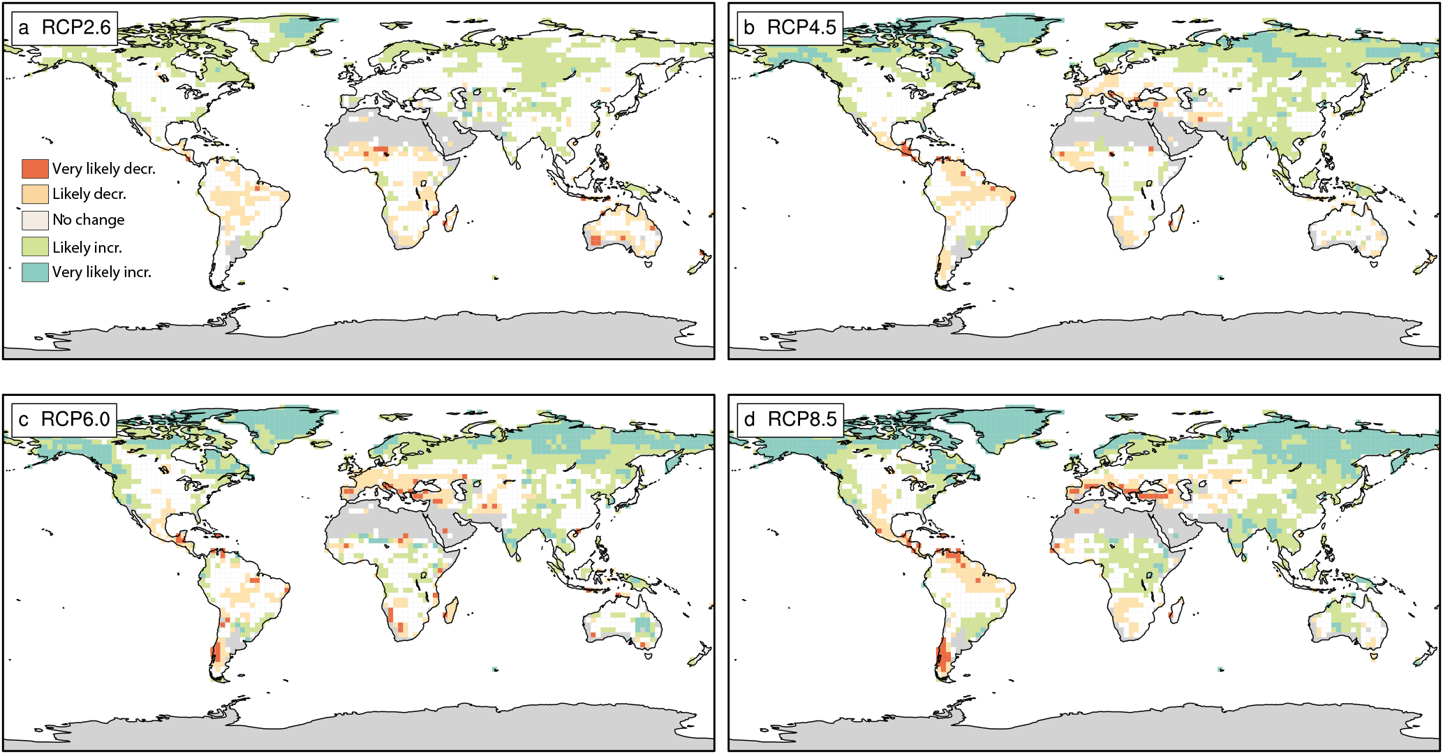
Figure 6Conceptual summary of the probability that the slope of P − E is negatively/positively different from zero considering all climate models and (a) the RCP2.6, (b) the RCP4.5, (c) RCP6.0 and (d) RCP8.5 emission scenarios only. See Fig. 4 for comparison.

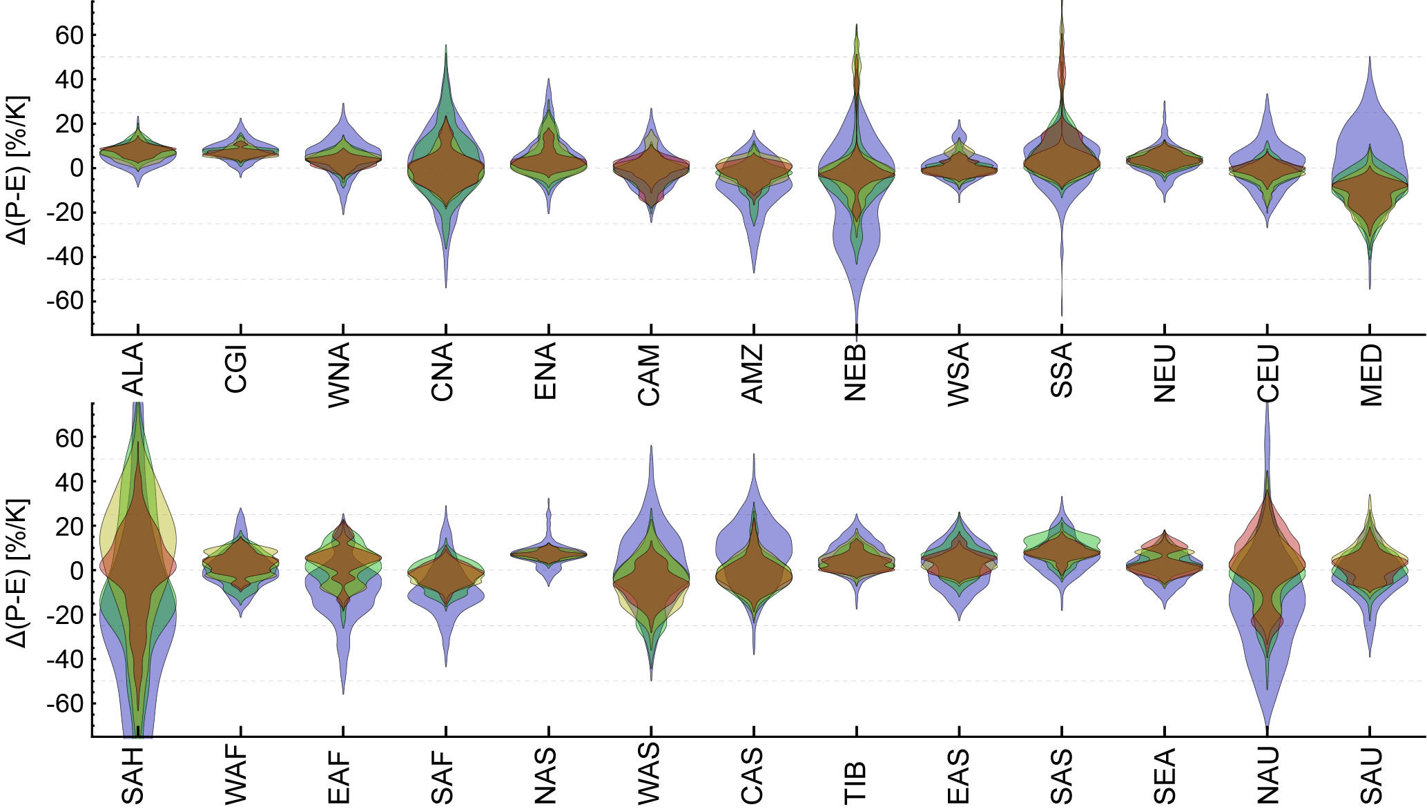
Figure 8Uncertainty distributions (shown as violin plots) of the sensitivity of P − E to global mean temperature change for each emission scenario averaged over all SREX regions (as outlined in Table 2 and Fig. 4). It is important to note that the data considered to estimate the area average are scarce in some regions (e.g. SAH). Please also refer to Fig. 7 for more information.
Considering the total uncertainty across all models and scenarios and by additionally including the internal variability, we are able to estimate the uncertainty distribution of the regional scaling coefficient of P and P − E against globally averaged T. Displayed in Fig. 2 are the median and the 10th and 90th quantiles of the uncertainty distribution of the scaling coefficient for both P and P − E at each grid point. The median scaling coefficient shows positive values, and hence an increase in both P and P − E with increasing T, in most parts of the northern high latitudes and Asia, but also in eastern Africa for both P and P − E. Negative values, and hence a decrease in both P and P − E with increasing T, are found in the Mediterranean region, southern Africa, Australia and in parts of west Africa, as well as Central and South America. Comparing the 10th and 90th quantiles of the uncertainty distribution shows the range of possible scaling coefficients. This range does, in most regions and especially for P − E, include the zero coefficient, which means that the probability of experiencing a scaling response of a different sign compared to the median response is 10 % or higher. The range is further generally much larger for P − E, pointing towards overall higher uncertainties in the estimation of the scaling relationship. The range is especially large in most subtropical regions (the Sahara, Arabian Peninsula, India, Australia, etc.). Regions showing a significant increase of P and P − E with global warming are located mainly in the northern high latitudes.
Figure 3 summarizes these findings by qualitatively showing the probability of experiencing either a positive or negative scaling response in P with respect to global warming. A very likely increase (90–100 % probability) in regional P with ongoing global warming is hence found only within grid cells of the northern high latitudes, whereas a likely increase (66–100 % probability) is located also in many parts of Asia and North America and to a minor extent also in some regions of South America and Africa. A likely decrease is located in most parts of the Mediterranean region, southern Africa, northeastern South America, Central America and along the Australian coastal regions. A decrease that is very likely is only found in South Africa. Most other regions show either uncertainty or no change. Figure 3 also illustrates selected quantiles of the uncertainty distribution of the scaling coefficient of P against global temperature increase for a comprehensive subset of SREX (Special Report on Managing the Risks of Extreme Events and Disasters to Advance Climate Change Adaptation) regions (Seneviratne et al., 2012) as outlined in the map (see also Table 2 for more information). Very certain responses within the SREX regions are only found for those in the northern high latitudes (ALA, NAS, NEU), while most other regions show a large spread of the uncertainty distribution (especially, e.g. in NEB, NAU).
Similarly for P − E, Fig. 4 displays a very likely increase (90–100 % probability) in regional P − E with ongoing global warming for an even smaller portion of land in the northern high latitudes, whereas a likely increase (66–100 % probability) is located throughout the northern high latitudes and similarly to P in many parts of Asia and North America and to a minor extent also in some regions in South America and Africa. A likely decrease is located in parts of the Mediterranean region, southern Africa, northeastern South America, Central America and some parts of Australia. A very likely decrease is only found for single grid points, primarily in Central America. Most other (and when compared to P an even higher number of) regions show either uncertainty or no change. Figure 4 also illustrates selected quantiles of the uncertainty distribution of the scaling coefficient of P − E with global temperature increase for the same set of SREX regions as shown in Fig. 3. Very certain responses are again only found in the northern high latitudes (ALA, NAS) and southern Asia (SAS), while most other regions show a very large and even larger spread of the uncertainty distribution when compared to estimates of P.
Please note that the results for both P and P − E are neither substantially influenced by the unequal number of available models per scenario nor individual climate models of the ensemble that potentially exhibit a large hydroclimatological drift (Liepert and Lo, 2013; Liepert and Previdi, 2012) (see Figs. 3–8).
3.1 Scenario uncertainty
The probability of experiencing an increase or decrease in regional P and P − E with global warming depends on the emission scenario. At global scales, mean precipitation scaling was shown to depend on the emission scenario (Andrews et al., 2009; Frieler et al., 2011; Pendergrass and Hartmann, 2012; Pendergrass et al., 2015), whereas the scaling of extreme precipitation is independent of the emission scenario (Pendergrass et al., 2015; Seneviratne et al., 2016). Here, we assess the relationship of regional changes in P and P − E on the emission scenario by analysing the uncertainty distributions of the scaling coefficient for each scenario individually. A conceptual representation of the probability of the scaling coefficient being positive/negative is displayed for P in Fig. 5 and for P − E in Fig. 6 (similar to the total uncertainty as shown in Figs. 3 and 4). In general, the fraction of regions showing either likely or very likely changes is increasing with the emission scenario for both P and P − E, pointing towards a larger uncertainty in the estimation of the scaling coefficient in the event that the climate change forcing is weak (RCP2.6, RCP4.5). Further, regions showing very likely changes are more common under high emission scenarios (RCP6.0, RCP8.5). The drying response in the Mediterranean region is, e.g. not evident when considering the RCP2.6 scenario alone, whereas a very likely decrease is found in the RCP8.5 scenario. In fact, individual grid points of the Mediterranean region (e.g. in central Spain) even show a likely increase in P and P − E in the RCP2.6 scenario. On the other hand, a likely drying response in parts of central and northern Australia found in RCP2.6 disappears for higher emission scenarios for P, or even turns into a wetting response for P − E. Robust signals are, again, found in most parts of the northern high latitudes, showing a (very) likely increase across all emission scenarios. A (very) likely decrease across all scenarios is further found for parts of southern Africa and parts of the Amazon region. Also note here that the overall conclusions for both P and P − E are not influenced by the unequal number of available models per scenario (please see Figs. S3–6).
A more detailed look at the underlying uncertainty distributions for P and P − E within each SREX region is provided in Figs. 7 and 8, respectively. It is clearly evident that the uncertainty is largest for low emission scenarios throughout all regions and in most cases lowest for the RCP8.5 scenario (with overall larger uncertainties in P − E; please note the different y-axis scales). Additionally, the uncertainty distribution of the higher emission scenarios is usually situated within the uncertainty range of the low emission scenarios, pointing towards a more robust signal. However, there are often large differences regarding the median response and the location and shape of the uncertainty distribution of a particular emission scenario with respect to other emission scenarios. This is especially evident when comparing low to high emission scenarios. Most prominently, for many regions (e.g. WNA, CAM, MED, WAS, CAS; please see Table 2 for more information on the acronyms), the uncertainty distribution of the RCP6.0 or RCP8.5 scenarios is located mainly within the lowest tercile of the RCP2.6 scenario, leading to a dryer response in P and P − E with global warming for high emission scenarios. This finding is, however, reversed in a few other regions (especially NAU and for P − E, and to a certain extent, also in ALA, EAF, SEA). The shapes of the uncertainty distributions for both P and P − E are also different between regions and emission scenarios. While the distributions for the low emission scenarios are, in most cases, unimodal, there are bimodal distributions in some (e.g. for P: NEU, WAS, CAS; for P − E: MED, EAS, SEA) and even multimodal distributions in a few other regions (e.g. for P: AMZ, NAS; for P − E: CNA, WAF, EAF) for the higher emission scenarios (especially RCP8.5). Please note, however, that not all models provide data for the RCP2.6 and RCP6.0 emission scenarios, which might also cause differences in the distributional shapes between those and the other scenarios (see Table 1 for more information).
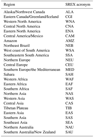
Table 2List of acronyms for all 26 SREX regions (Seneviratne et al., 2012).
3.2 Comparing different sources of uncertainty
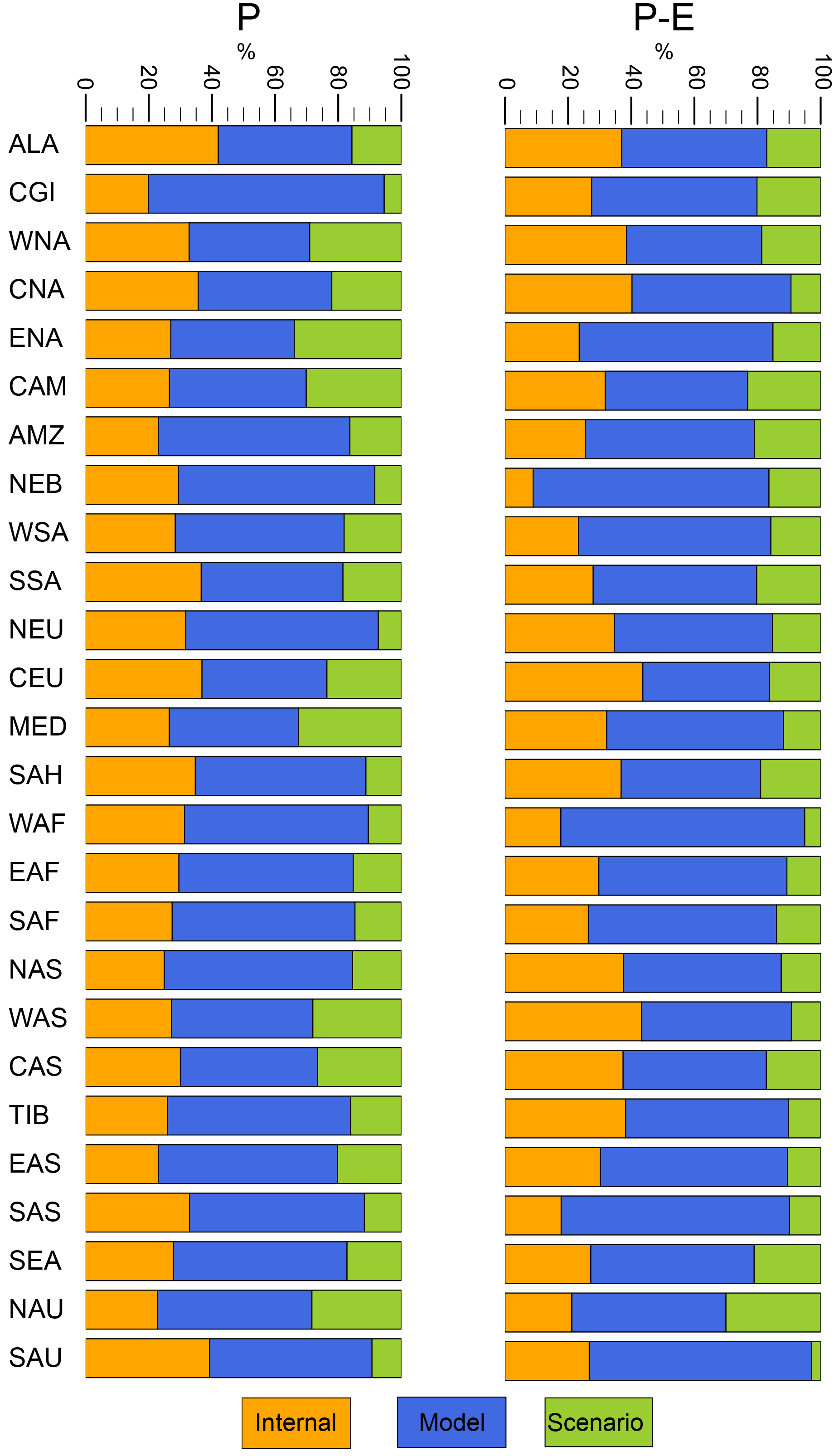
Besides the scenario uncertainty, we also introduced two other sources of uncertainty in Sect. 2: the internal variability and the model uncertainty, which contribute to the total uncertainty. Here, we assess the fraction of uncertainty which each source contributes to the total uncertainty. We follow the approach of Hawkins and Sutton (2009), which was also adapted in Orlowsky and Seneviratne (2013). Therefore, we compare (i) the average over the variances of the uncertainty distributions of each model under each emission scenario (internal uncertainty, σi), (ii) the average of the variances of scenario-specific uncertainty distributions of each model (model uncertainty, σm) and (iii) the variance of the averages of all uncertainty distributions within a specific scenario (scenario uncertainty, σs). Even though this approach of attributing uncertainties is very simplistic (see Sect. 2), it provides basic information on the composition of different uncertainty sources within the total uncertainty. The percentage of the total uncertainty that stems from a particular source is illustrated for both P and P − E in Fig. 9. For all SREX regions, there is generally no single source of uncertainty contributing more than 80 % to the total uncertainty. However, in most regions, the largest source of uncertainty stems from model uncertainty, which is contributing up to approximately ca. three-fourths of the total uncertainty in some regions and is especially large in most northern high-latitude regions (CGI, NEU, NAS, except ALA). Internal variability contributes between 20 and 40 % to the total uncertainty, with highest values found in particular for several regions adjacent to the Pacific Ocean (e.g. WNA, SEA, SAU). Internal variability seems to be rather low in other tropical to subtropical regions, such as AMZ, EAS and NAU for P and NEB, WAF and SAS for P − E. Scenario uncertainty contributes between approximately 5 and 30 % to the total uncertainty with those regions reaching highest values that have differing locations of the uncertainty distributions between low and high emission scenarios as shown in Figs. 7 and 8 (e.g. WNA, ENA, CAM, MED, WAS, CAS and NAU). Differences in P between emission scenarios are further not solely caused by varying radiative forcing due to differing greenhouse gas emissions, but also due to differences in the black carbon forcing (Pendergrass and Hartmann, 2012). It is further interesting to note that scenario uncertainty is generally lower and internal variability generally larger for P − E when compared to P. However, even though the scenario uncertainty is the overall weakest source of uncertainty in most regions, it is by no means negligible. Please note, again, that the scenario uncertainty interferes especially with the rather large model uncertainty and we do not account for such relationships in this approach.
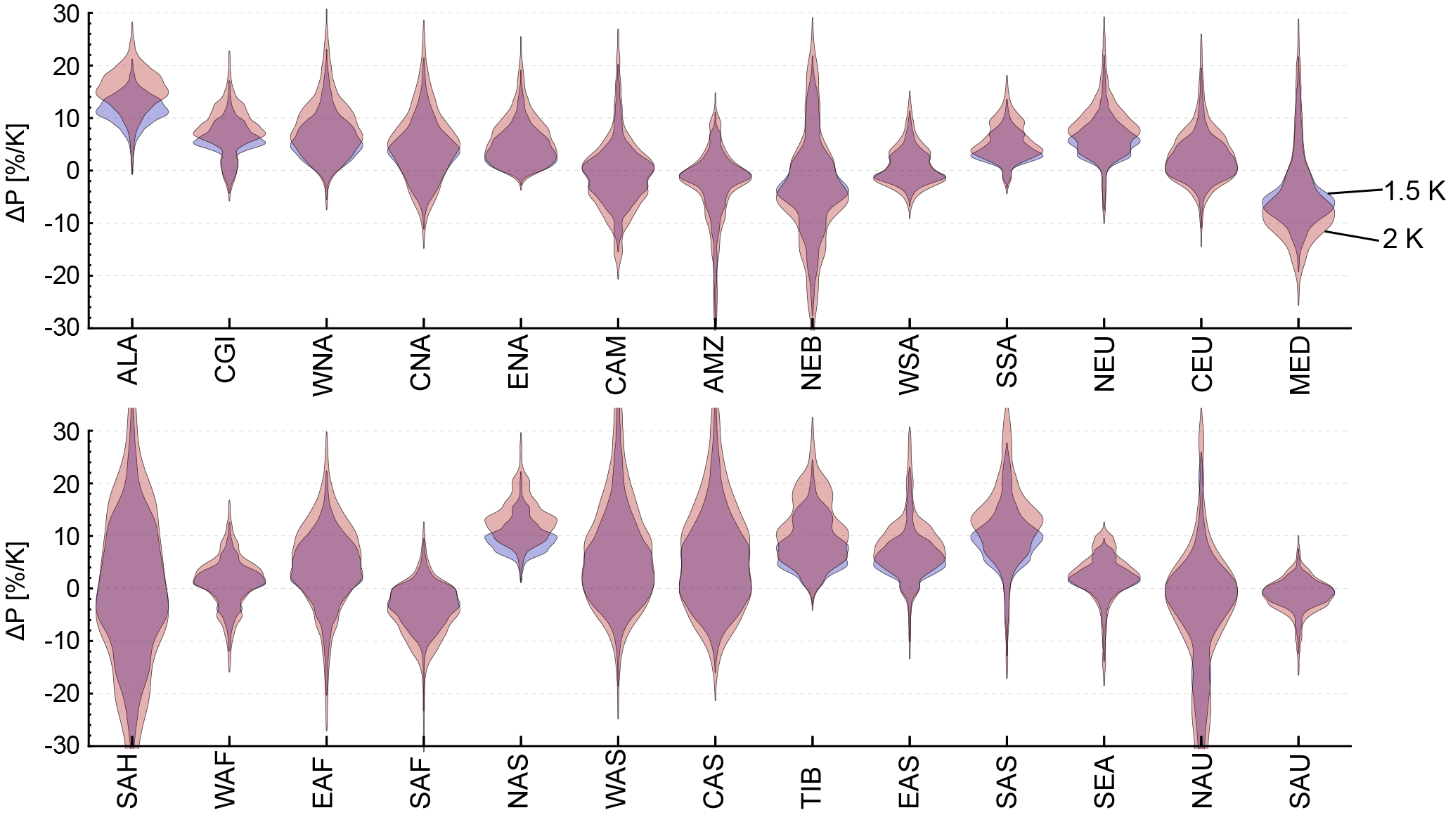
Figure 10Uncertainty distributions (shown as violin plots) of the sensitivity of P to global mean temperature change for two different degrees of global mean temperature change, which correspond to the widely used warming-degree limits of 1.5 and 2 K. The estimates are averaged over all SREX regions (as outlined in Fig. 3 and Table 2).

Figure 11Uncertainty distributions (shown as violin plots) of the sensitivity of P − E to global mean temperature change for two different degrees of global mean temperature change, which correspond to the widely used warming-degree limits of 1.5 and 2 K. The estimates are averaged over all SREX regions (as outlined in Fig. 3 and Table 2). It is important to note that the data considered to estimate the area average are scarce in some regions (e.g. SAH). Please also refer to Fig. 10 for more information.
As agreed at COP21, the increase in global mean temperature should be limited to values well below the previously set goal of 2 K, preferably to not more than 1.5 K above pre-industrial conditions. However, global mean temperature is an abstract value and provides no information about direct implications at regional scales and with respect to other climate variables such as regional, mean-annual P or P − E. The framework developed within this study enables us to directly assess the regional response of P and P − E to these targets and to study differences between them. Using the uncertainty distributions of each SREX region and scaling them to either 1.5 or 2 K (as illustrated in Fig. 10 for P and in Fig. 11 for P − E) allows us to study differences both in the median response as well as in the tails of the distribution. It is, however, naturally evident that in regions with a weak median scaling response the difference between the warming-degree targets is small regarding the median response itself (e.g. AMZ, CEU, WAS), whereas in regions with a stronger median scaling (e.g. ALA, NEU, NAS) an additional 0.5 K warming could lead to substantial differences. Nonetheless, even though the difference in the median might be small, the differences in the tails of the uncertainty distributions are in most cases significant and stress an increased risk of experiencing strong changes in P and P − E. As an example for the Mediterranean region (MED), the median responses of P to 1.5 K global warming vs. 2 K global warming are not strongly different, while there are stronger differences at the tails, showing that the 1.5 K limit would avoid a decrease of P by more than 20 %, which, on the other hand, cannot be excluded with the 2 K limit. This behaviour is even more evident for P − E and also occurs in regions with almost no median response (e.g. CEU). Also the irregularity of the distribution further amplifies this behaviour in some regions. In summary, opting for a low warming-degree target (such as 1.5 K) might just slightly influence the mean response but could substantially reduce the risk of experiencing more extreme changes in regional P and P − E.
We developed here a framework building upon the pattern scaling approach to assess regional changes in mean-annual P and P − E with respect to global mean T increase by utilizing a comprehensive subset of climate models and considering all available emission scenarios. We further took into account internal variability from each projection by accounting for the year-to-year variability of P and P − E. This enabled us to assess a conservative estimate of the uncertainty distribution of the scaling coefficient of P and P − E to global warming at every grid point or within SREX regions.
Analysing maps of the median response and the responses in the 10th and 90th quantiles of the grid-point-specific uncertainty distributions showed low uncertainties and positive scaling coefficients (thereby a certain increase in P and P − E with global warming) within most northern high-latitude regions. Slight decreases in the median response together with large uncertainties (and thereby an uncertain decrease in P and P − E with global warming) are found for most subtropical regions. Uncertainties are, however, larger for estimates of P − E and hence do not permit robust conclusions for many regions. Our results support previous findings of hydroclimatological changes (Greve and Seneviratne, 2015), but provide a new, probabilistic and rigorous perspective on the assessment of uncertainties in regional hydroclimatological changes under conditions of ongoing global warming and extend the wealth of studies investigating pattern scaling approaches of climate variables (Herger et al., 2015; Tebaldi and Arblaster, 2014).
Assessing scenario-specific uncertainty distributions revealed strong regional differences between different emission scenarios. It is evident that weaker climate change signals within the low-emission scenarios (RCP2.6, RCP4.5) lead to high uncertainties in the estimation of scaling coefficients. A very likely change in regional P only emerges under high emission scenarios (RCP6.0, RCP8.5) and is even less likely to occur for P − E. In some regions, low emission scenarios further show likely opposite changes compared to changes identified in higher emission scenarios (both switching from a likely wetting response to a very likely drying response in parts of MED, or from a likely drying response to no change in P or even a likely wetting response in P − E in NAU). A closer look a the uncertainty distributions shows large differences both in location and shape across regions and emission scenarios. However, in most cases, higher emission scenarios point towards a dryer response than low emission scenarios (with a few regions showing, however, the opposite behaviour).
This led us to the analysis of the relative contribution of single sources of uncertainty to the overall uncertainty. It is shown that model uncertainty is largest in most regions, but is, however, in no case contributing more than 80 % to the overall uncertainty. It is therefore important that both internal variability and scenario uncertainty are considered as well in order to get a complete picture of the total uncertainty. Comparing mean-annual P and P − E shows that scenario uncertainty is generally lower and internal variability generally larger for P − E.
We further assessed the implications of different warming-degree limits on changes in regional P and P − E. At the COP21, most nations agreed to limit the increase in global mean temperature to values well below the previously set goal of 2 K and to consider limiting warming to not more than 1.5 K above pre-industrial conditions. Comparing these two targets reveals little differences in the mean response in regions where the mean response is small anyway. However, since uncertainties are large, especially for P − E, there is a nonlinear increase in the risk of experiencing more extreme changes. Therefore, opting for a low warming-degree target (such as 1.5 K) might just slightly influence the mean response but could substantially reduce the risk of experiencing extreme changes in regional P and P − E. This means that even though the discussion about the implications of 1.5 K vs. 2 K global warming might be moot for the mean response, it is, given the underlying large uncertainties of climate projections, absolutely necessary to more closely investigate the potentially large increase in the risk of experiencing extreme change. This is especially important in order to enable robust decision-making to ensure adequate development pathways and to avoid the risk of maladaptation; in the specific case of changes in mean-annual P and P − E, this is, e.g. of high relevance for water resources managers and farmers.
We acknowledge the World Climate Research Programme's Working Group on Coupled Modelling, which is responsible for the Coupled Model Intercomparison Project (CMIP), and we thank the climate modelling groups for producing and making available their model output. For CMIP, the US Department of Energy's Program for Climate Model Diagnosis and Intercomparison provides coordinating support and led development of software infrastructure in partnership with the Global Organization for Earth System Science Portals. The data used in this study are available through the Coupled Model Intercomparison Project Phase 5 at https://esgf-node.llnl.gov/projects/esgf-llnl/.
The supplement related to this article is available online at: https://doi.org/10.5194/esd-9-227-2018-supplement.
The authors declare that they have no conflict of interest.
We thank Jakob Zscheischler for providing useful input regarding methodological
aspects of this study and Urs Beyerle and Jan Sedlacek for processing the CMIP5 data.
Edited by: Christian Franzke
Reviewed by: three anonymous referees
Andrews, T., Forster, P. M., and Gregory, J. M.: A Surface Energy Perspective on Climate Change, J. Climate, 22, 2557–2570, https://doi.org/10.1175/2008JCLI2759.1, 2009. a, b, c
Fischer, E. M., Sedláček, J., Hawkins, E., and Knutti, R.: Models agree on forced response pattern of precipitation and temperature extremes, Geophys. Res. Lett., 41, 8554–8562, https://doi.org/10.1002/2014GL062018, 2014. a, b
Frieler, K., Meinshausen, M., Schneider von Deimling, T., Andrews, T., and Forster, P.: Changes in global-mean precipitation in response to warming, greenhouse gas forcing and black carbon, Geophys. Res. Lett., 38, L04702, https://doi.org/10.1029/2010GL045953, 2011. a, b, c
Good, P., Booth, B. B. B., Chadwick, R., Hawkins, E., Jonko, A., and Lowe, J. A.: Large differences in regional precipitation change between a first and second 2 K of global warming, Nat. Commun., 7, 13667, https://doi.org/10.1038/ncomms13667, 2016. a
Greve, P. and Seneviratne, S. I.: Assessment of future changes in water availability and aridity, Geophys. Res. Lett., 42, 5493–5499, https://doi.org/10.1002/2015GL064127, 2015. a
Guiot, J. and Cramer, W.: Climate change: The 2015 Paris Agreement thresholds and Mediterranean basin ecosystems, Science, 354, 465–468, https://doi.org/10.1126/science.aah5015, 2016. a
Hawkins, E. and Sutton, R.: The Potential to Narrow Uncertainty in Regional Climate Predictions, B. Am. Meteorol. Soc., 90, 1095–1107, https://doi.org/10.1175/2009BAMS2607.1, 2009. a
Herger, N., Sanderson, B. M., and Knutti, R.: Improved pattern scaling approaches for the use in climate impact studies, Geophys. Res. Lett., 42, 3486–3494, https://doi.org/10.1002/2015GL063569, 2015. a, b
James, R., Washington, R., Schleussner, C.-F., Rogelj, J., and Conway, D.: Characterizing half-a-degree difference: a review of methods for identifying regional climate responses to global warming targets, WIREs Clim. Change, 8, e457, https://doi.org/10.1002/wcc.457, 2017. a
Knutti, R., Rogelj, J., Sedláček, J., and Fischer, E. M.: A scientific critique of the two-degree climate change target, Nat. Geosci., 9, 13–18, https://doi.org/10.1038/ngeo2595, 2016. a
Kravitz, B., Lynch, C., Hartin, C., and Bond-Lamberty, B.: Exploring precipitation pattern scaling methodologies and robustness among CMIP5 models, Geosci. Model Dev., 10, 1889–1902, https://doi.org/10.5194/gmd-10-1889-2017, 2017. a
Liepert, B. G. and Lo, F.: CMIP5 update of `Inter-model variability and biases of the global water cycle in CMIP3 coupled climate models', Environ. Res. Lett., 8, 029401, https://doi.org/10.1088/1748-9326/8/2/029401, 2013. a
Liepert, B. G. and Previdi, M.: Inter-model variability and biases of the global water cycle in CMIP3 coupled climate models, Environ. Res. Lett., 7, 014006, https://doi.org/10.1088/1748-9326/7/1/014006, 2012. a
Mitchell, T. D.: Pattern Scaling: An Examination of the Accuracy of the Technique for Describing Future Climates, Climatic Change, 60, 217–242, https://doi.org/10.1023/A:1026035305597, 2003. a
Moss, R. H., Edmonds, J. A., Hibbard, K. A., Manning, M. R., Rose, S. K., van Vuuren, D. P., Carter, T. R., Emori, S., Kainuma, M., Kram, T., Meehl, G. A., Mitchell, J. F. B., Nakicenovic, N., Riahi, K., Smith, S. J., Stouffer, R. J., Thomson, A. M., Weyant, J. P., and Wilbanks, T. J.: The next generation of scenarios for climate change research and assessment, Nature, 463, 747–756, https://doi.org/10.1038/nature08823, 2010. a
Orlowsky, B. and Seneviratne, S. I.: Elusive drought: uncertainty in observed trends and short- and long-term CMIP5 projections, Hydrol. Earth Syst. Sci., 17, 1765–1781, https://doi.org/10.5194/hess-17-1765-2013, 2013. a
Pendergrass, A. G. and Hartmann, D. L.: Global-mean precipitation and black carbon in AR4 simulations, Geophys. Res. Lett., 39, L01703, https://doi.org/10.1029/2011GL050067, 2012. a, b, c, d
Pendergrass, A. G., Lehner, F., Sanderson, B. M., and Xu, Y.: Does extreme precipitation intensity depend on the emissions scenario?, Geophys. Res. Lett., 42, 8767–8774, https://doi.org/10.1002/2015GL065854, 2015. a, b, c, d, e
Santer, B., Wigley, M., Schlesinger, M., and Mitchell, J.: Developing climate scenarios from equilibrium GCM results, Tech. Rep., Hamburg, Germany, 1990. a
Schleussner, C.-F., Lissner, T. K., Fischer, E. M., Wohland, J., Perrette, M., Golly, A., Rogelj, J., Childers, K., Schewe, J., Frieler, K., Mengel, M., Hare, W., and Schaeffer, M.: Differential climate impacts for policy-relevant limits to global warming: the case of 1.5 ∘C and 2 ∘C, Earth Syst. Dynam., 7, 327–351, https://doi.org/10.5194/esd-7-327-2016, 2016. a
Seneviratne, S. I., Nicholls, N., Easterling, D., Goodess, C., Kanae, S., Kossin, J., Luo, Y., Marengo, J., McInnes, K., Rahimi, M., Reichstein, M., Sorteberg, A., Vera, C., and Zhang, X.: Changes in climate extremes and their impacts on the natural physical environment, in: Managing the Risks of Extreme Events and Disasters to Advance Climate Change Adaptation, A Special Report of Working Groups I and II of the Intergovernmental Panel on Climate Change, edited by: Field, C. B., Barros, V., Stocker, T. F., Qin, D., Dokken, D. J., Ebi, K. J., Mastrandrea, M. D., Mach, K. J., Plattner, G.-K., Allen, S. K., Tignor, M., and Midgley, P. M., IPCC, Cambridge University Press, Cambridge, UK, and New York, NY, USA, 2012. a, b
Seneviratne, S. I., Donat, M. G., Pitman, A. J., Knutti, R., and Wilby, R. L.: Allowable CO2 emissions based on regional and impact-related climate targets, Nature, 529, 477–483, https://doi.org/10.1038/nature16542, 2016. a, b, c, d, e
Solomon, S., Plattner, G.-K., Knutti, R., and Friedlingstein, P.: Irreversible climate change due to carbon dioxide emissions, P. Natl. Acad. Sci. USA, 106, 1704–1709, https://doi.org/10.1073/pnas.0812721106, 2009. a
Taylor, K., Stouffer, R., and Meehl, G.: An Overview of CMIP5 and the Experiment Design, B. Am. Meteorol. Soc., 93, 485–498, https://doi.org/10.1175/BAMS-D-11-00094.1, 2012. a
Tebaldi, C. and Arblaster, J. M.: Pattern scaling: Its strengths and limitations, and an update on the latest model simulations, Climatic Change, 122, 459–471, https://doi.org/10.1007/s10584-013-1032-9, 2014. a, b, c
Victor, D. G. and Kennel, C. F.: Climate policy: Ditch the 2 ∘C warming goal, Nature News, 514, 30–31, https://doi.org/10.1038/514030a, 2014. a
Wartenburger, R., Hirschi, M., Donat, M. G., Greve, P., Pitman, A. J., and Seneviratne, S. I.: Changes in regional climate extremes as a function of global mean temperature: an interactive plotting framework, Geosci. Model Dev., 10, 3609–3634, https://doi.org/10.5194/gmd-10-3609-2017, 2017. a, b, c