the Creative Commons Attribution 4.0 License.
the Creative Commons Attribution 4.0 License.
 | 20 Aug 2018
A theory of Pleistocene glacial rhythmicity
Mikhail Y. Verbitsky
Michel Crucifix
Dmitry M. Volobuev
Variations in Northern Hemisphere ice volume over the past 3 million years have been described in numerous studies and well documented. These studies depict the mid-Pleistocene transition from 40 kyr oscillations of global ice to predominantly 100 kyr oscillations around 1 million years ago. It is generally accepted to attribute the 40 kyr period to astronomical forcing and to attribute the transition to the 100 kyr mode to a phenomenon caused by a slow trend, which around the mid-Pleistocene enabled the manifestation of nonlinear processes. However, both the physical nature of this nonlinearity and its interpretation in terms of dynamical systems theory are debated. Here, we show that ice-sheet physics coupled with a linear climate temperature feedback conceal enough dynamics to satisfactorily explain the system response over the full Pleistocene. There is no need, a priori, to call for a nonlinear response of the carbon cycle. Without astronomical forcing, the obtained dynamical system evolves to equilibrium. When it is astronomically forced, depending on the values of the parameters involved, the system is capable of producing different modes of nonlinearity and consequently different periods of rhythmicity. The crucial factor that defines a specific mode of system response is the relative intensity of glaciation (negative) and climate temperature (positive) feedbacks. To measure this factor, we introduce a dimensionless variability number, V. When positive feedback is weak (V∼0), the system exhibits fluctuations with dominating periods of about 40 kyr which is in fact a combination of a doubled precession period and (to smaller extent) obliquity period. When positive feedback increases (V∼0.75), the system evolves with a roughly 100 kyr period due to a doubled obliquity period. If positive feedback increases further (V∼0.95), the system produces fluctuations of about 400 kyr. When the V number is gradually increased from its low early Pleistocene values to its late Pleistocene value of V∼0.75, the system reproduces the mid-Pleistocene transition from mostly 40 kyr fluctuations to a 100 kyr period rhythmicity. Since the V number is a combination of multiple parameters, it implies that multiple scenarios are possible to account for the mid-Pleistocene transition. Thus, our theory is capable of explaining all major features of the Pleistocene climate, such as the mostly 40 kyr fluctuations of the early Pleistocene, a transition from an early Pleistocene type of nonlinear regime to a late Pleistocene type of nonlinear regime, and the 100 kyr fluctuations of the late Pleistocene.
When the dynamical climate system is expanded to include Antarctic glaciation, it becomes apparent that climate temperature positive feedback (or its absence) plays a crucial role in the Southern Hemisphere as well. While the Northern Hemisphere insolation impact is amplified by the outside-of-glacier climate and eventually affects Antarctic surface and basal temperatures, the Antarctic ice-sheet area of glaciation is limited by the area of the Antarctic continent, and therefore it cannot engage in strong positive climate feedback. This may serve as a plausible explanation for the synchronous response of the Northern and Southern Hemisphere to Northern Hemisphere insolation variations.
Given that the V number is dimensionless, we consider that this model could be used as a framework to investigate other physics that may possibly be involved in producing ice ages. In such a case, the equation currently representing climate temperature would describe some other climate component of interest, and as long as this component is capable of producing an appropriate V number, it may perhaps be considered a feasible candidate.
- Article
(4216 KB) - Full-text XML
- BibTeX
- EndNote


Existing empirical records provide significant evidence that glacial oscillations during the last 3 million years experienced major change in their modes of rhythmicity, switching from predominately nearly 40 kyr period fluctuations of the early Pleistocene to about 100 kyr oscillations in the late Pleistocene. During the last 50 years, considerable efforts of the scientific community have been directed to the explanation of these phenomena. A systematic review of the last century's work was presented by Saltzman (2002) in his last book. An insightful overview of more recent efforts can be found, for example, in Clark et al. (2006), Tziperman et al. (2006), Crucifix (2013), Mitsui and Aihara (2014), Paillard (2015), and Ashwin and Ditlevsen (2015). As of today, it is widely acknowledged that 23 and 40 kyr fluctuations of Pleistocene global ice volume represent a climate system response to astronomical forcing on precession and obliquity frequency bands. At the same time, the causes of major late Pleistocene 100 kyr oscillations and the explanation for the physics that led to the transition from the 40 kyr period to the 100 kyr period remain unsettled.
In some previous work (Saltzman and Verbitsky, 1992, 1993a, b; 1994a, b) we attempted to explain the nature of Pleistocene ice ages using a dynamical global climate model describing the evolution of global ice mass, bedrock depression, atmospheric carbon dioxide concentration, and ocean temperature. The central piece of this model was the ice–carbon dioxide oscillator, which produced 100 kyr cycles. As a justification, we considered the evolution of the global climate system on a phase plane using empirical data of global ice volume against records of carbon dioxide concentration (Saltzman and Verbitsky, 1994a). This phase diagram supported our assumption that carbon dioxide leads ice volume changes. Other authors have advanced similar proposals. For example, Paillard and Parrenin (2004) present a simple model of ice-sheet–ocean and carbon cycle dynamics. The nonlinear terms, which are necessary to generate the mid-Pleistocene transition and the 100 ka mode, are located in the ocean and carbon cycle equations. However, this explanation needs to be challenged. First, a detailed discussion of the timing of CO2 and the benthic isotopic record leaves open the possibility that at the timescale of the glacial–interglacial cycle the CO2 simply acts as a feedback on ice volume (Ruddiman, 2006), even if it is also observed that the dynamics of the deglaciation are complex and that CO2 changes can go through fairly abrupt dynamics (Ganopolski and Roche, 2009). On the other hand, other potential elements in the Earth system could generate nonlinearities yielding 100 kyr cycles: Ashkenazy and Tziperman (2004) proposed a “sea-ice switch”, Imbrie et al. (2011) interpret the nonlinear terms of their models as a representation of ice-sheet instability, Ellis and Palmer (2016) consider a dust albedo feedback, and Omta et al. (2016) invoke an instability of the carbonate cycle. There is a plethora of possible mechanisms, but the mathematical expression of these various mechanisms is scarcely firmly constrained. The physical cause of ice-age cycles remains, for that reason, largely contentious. In parallel, simulations based on models with more physically and geographically explicit models, such as the models of intermediate complexity of Verbitsky and Chalikov (1986), Chalikov and Verbitsky (1990), and Ganopolski et al. (2010) and the higher-resolution ice-sheet–climate model of Abe-Ouchi et al. (2013), confirm the important role of ice-sheet dynamics in shaping the 100 kyr cycle.
In this paper, our aim is to approach this question from a different perspective. The approach proposed here is both reductionist – we rely on laws of thermo-hydrodynamics – and parsimonious: we intend to explain the phenomenon of interest (the apparition and repetition of ice-age cycles) with a minimal set of assumptions. We limit ourselves to just two components that, without a doubt, should be part of any ice-age story: ice sheets and the ocean representing the rest of the climate. With this constraint, we derive a simple dynamical system using scaled equations of ice-sheet thermodynamics and combine them with an equation describing the evolution of climate temperature. The model obtained is a nonlinear dynamical system incorporating three variables: area of glaciation, ice-sheet basal temperature, and characteristic temperature of outside-of-glacier climate. Since we derive model equations from the conservation laws, all system parameters are at least partly constrained. Some of them are based on empirical data of present ice sheets and others can be calibrated with a three-dimensional ice-sheet model and global general circulation climate models.
Without astronomical forcing, this system evolves to equilibrium. When it is astronomically forced, it may produce different modes of rhythmicity (including periods of 23, 40, 100, and 400 kyr). We will show that the critical system property that defines system response to astronomical forcing is a specific balance between the intensities of the positive and negative feedbacks involved. We will evaluate this balance with a variability number (V number), a dimensionless combination of eight model parameters measuring the relative intensity of climate temperature (positive) and glaciation (negative) feedbacks. We will demonstrate that, depending on the V number, the mechanism of nonlinear amplification of the astronomical forcing will produce different results. We will also show that asymmetry of the climate positive feedback may be a critical factor in explaining the synchronous response of the Northern and Southern Hemisphere to Northern Hemisphere insolation variations.
Accordingly, our paper is organized as follows. First we will derive simple equations representing continental glaciation and test their parameters using sensitivity experiments with a three-dimensional model of the Antarctic ice sheet. We will then combine ice-sheet and climate temperature equations into a dynamical model of the glacial cycles and analyze its properties. We will inspect all feedbacks present in the system and suggest a dimensionless criterion (V number) that measures their relative intensity. We will then model our system response to astronomical forcing for different V numbers to reproduce early and late Pleistocene modes of glacial rhythmicity as well as the mid-Pleistocene transition. Finally, we will expand our system to include Antarctic glaciation.
As we have explained in the Introduction, our ambition is to follow a parsimonious approach but rely on reductionism. To achieve this agenda, we will apply scaling analysis to conservation equations. Indeed, scaling analysis provides simple mathematical statements that do not compromise the integrity of physical laws. Accordingly, we begin with the mass, momentum, and heat conservation equations for a thin layer of homogeneous non-Newtonian ice.
Here, x and z are the horizontal and vertical coordinates, p is pressure, u and w are the horizontal and vertical velocity components, σxz is the shear stress, ρ is density, ci is heat capacity, g is the acceleration of gravity, k is the temperature diffusivity, and q is the heat of internal friction. For typical horizontal and vertical dimensions of ice sheets like Antarctic, Laurentide, or Greenland and for typical ice viscosity, the inertial forces are negligible relative to stress gradients, and motion equations with very high accuracy can be written in a quasi-static form (Eqs. 2–3) (Paterson, 1981; Verbitsky and Chalikov, 1986).
We will now start the process of scaling Eqs. (1)–(4). We introduce the horizontal scale of the ice-sheet L, the scale of its thickness H, and the scale of the vertical velocity W=a, where a is the scale of the mass influx (net snow accumulation). From the continuity Eq. (1) and hydrostatic Eq. (3) we obtain the scale of the horizontal velocity and the scale of the pressure P=ρgH. From the momentum Eq. (2) we get the scale of the shear stress . The power rheological law 2μuz=σn (where μ is viscosity, uz is the strain rate, and n is power degree) provides us with an estimate . Since , and , where S is the glaciation area, we can finally get the scale of ice thickness (Vialov, 1958):
We start analysis of energy Eq. (4) with the notion that for typical glaciological systems the Peclet number is of order 10. This means that advection dominates the heat conservation Eq. (4) so that an ice-flow trajectory has a near-constant temperature determined by its value on the top surface of the ice sheet. We will now determine the thickness of the bottom boundary layer η, where vertical diffusion, kTzz, gains significance and is balanced by the advection of heat uTx. Using the scale of the horizontal velocity obtained above and assuming that vertical and horizontal temperature gradients are of the same order of magnitude, we have
Within this boundary layer, Eq. (4) can be reduced to
with boundary conditions T=Tη at z=η and at z=0. Here, λ=kρci is heat conductivity, and Q is the geothermal heat flux. Thus the scale of the basal temperature θ can be estimated as a sum of three scales.
The scale of the surface temperature effect is
Here, we account for the fact that Tη is “delivered” from the ice-sheet surface and can be estimated as TS−γH, where TS is the annual mean sea-level temperature, and γ is the vertical atmospheric lapse rate.
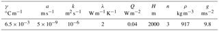
Table 1The values of physical parameters (Paterson, 1981; Verbitsky and Chalikov, 1986).
The scale of the internal friction effect is
The heat of the internal friction can be estimated as
Since , H is described by Eq. (5), and , then
Accounting for Eq. (6), the scale of the internal friction effect finally takes the form
The scale of the geothermal heat flux effect is
It can be seen now that the basal temperature θ is a function of ice thickness H, and because of Eq. (5), it is a function of snow precipitation intensity a and of viscosity μ. Since viscosity is temperature dependent, basal temperature is a function of ice temperature T. It is also function of climatic temperature TS and ice-sheet area S. Differentiating Eqs. (8), (12), and (13) along these variables provides us with estimates of basal temperature sensitivity to changing precipitations Δθa, climatic temperature ΔθT, and glaciation area ΔθS.
An asterisk (*) marks undisturbed values in the following sense: if y=f(x), then .
In deriving Eqs. (14)–(16), the temperature dependence of viscosity was adopted from Shumskiy (1975):
Here, ϑ=21.1, and Tm is the ice melting temperature (273.15 K). For simplicity, in Eqs. (14)–(16) we do not differentiate between T and TS.
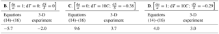
In calculating basal temperature response using the scaled Eqs. (14)–(16) we used the physical parameter values collected in Table 1.
It gives us the following sensitivities of basal temperature to external climatic factors.
It can be seen that when snow rate increases, intensified ice advection has a tendency to reduce the basal temperature (Δθa is negative) because it reduces the thickness of the basal boundary layer. Since snow rate usually increases with warmer climate, such a snow rate increase may at least partially compensate for a corresponding increase in basal temperature.
We tested Eqs. (14)–(16) using numerical experiments with the three-dimensional Antarctic ice-sheet model of Pollard and DeConto (2012a); see Appendix for details and full references. Though our research will be devoted mostly to Northern Hemisphere ice sheets like the Scandinavian or Laurentide, the Antarctic ice-sheet model can be a good analogue because it is governed by the same physics. In addition, temperature and snow precipitation rates for Antarctica are well known, unlike those for ancient ice sheets. Table A1 of the Appendix shows that the sign and order of magnitude of the basal temperature response to climatic forcing predicted by our scaling estimates are consistent with the results of the 3-D ice-sheet model.
We are now ready to formulate the dynamical model of the Pleistocene climate.
We will derive dynamical equations for three variables, namely the area of glaciation S, ice-sheet basal temperature θ, and characteristic temperature of outside-of-glacier climate ω.
3.1 Area of glaciation
We start with the mass conservation equation integrated over the entire ice-sheet surface:
Here, A is total snow accumulation minus ablation and calving. According to Eq. (5),
then, assuming ζ = const, Eq. (18) can be written as
It is interesting that the fundamental mass balance Eq. (19) provides some support for the hypothetical model of Huybers (2009). If we consider the right side of Eq. (19) to be the rate of deglaciation, then explicit finite differencing of Eq. (19) would give us
where the rate of deglaciation depends on the dimension of the previous glaciation, St−1. It does not imply that ice can “remember” its previous state; Eq. (19) simply tells us that deglaciation of bigger ice sheets occurs on a bigger area.
We adopt the following parameterization for the total mass balance A appearing in Eq. (19): .
Here, the following statements are true.
- a.
A1=a is the snow accumulation rate.
- b.
A2=εFS is the ice ablation rate due to astronomical forcing FS, the local mid-July insolation at 65∘ N (Berger and Loutre, 1991).
- c.
A3=κω is the ice ablation rate representing the cumulative effect of the global climate on ice-sheet mass balance. The variable ω is a characteristic temperature of outside-of-glacier climate. Accordingly, any climate-induced changes in ice-sheet mass balance are functions of ω. Increased climate temperature ω affects ice-sheet mass balance in several ways:
-
it changes (likely increases) snow precipitation;
-
it intensifies ablation;
-
it intensifies ice discharge due to reduced viscosity; and
-
corresponding changes in greenhouse gas concentration (CO2) affect the radiative balance of the atmosphere.
-
- d.
A4=cθ represents ice discharge due to ice-sheet basal sliding. The variable θ, which for simplicity we are going to call “basal temperature”, is in fact a measure of ice-sheet intensity of basal sliding. The basal temperature cannot exceed the melting point, but at that point, the continual influx of heat due to internal friction, geothermal heat flux, or heat from sliding can still increase the intensity of basal melting and facilitate sliding. This type of transition from the frozen bed to sliding conditions has been conceptually described by MacAyeal (1993) and further investigated by Payne (1995) and Marshall and Clark (2002) for the Laurentide ice sheet.
- e.
The parameters ε, κ, and c are sensitivity coefficients.
Accordingly, Eq. (19) takes the final form
3.2 Basal temperature
Scales (Eqs. 14–16) were obtained for the equilibrium state of the ice sheet. We now account for the fact that variations described by Eqs. (14)–(16) follow climate change with a time lag equal to a characteristic vertical advection rate H∕a:
We substitute scales (Eqs. 5 and 14–16) into Eq. (21). We combine Δθa and ΔθT together, assuming that Δθa is proportional to ΔθT and ΔθT is proportional to ω: . We replace in Eq. (16) with , where S0 is a reference glaciation area. Here, α and β are sensitivity coefficients. We also modify a like in Eq. (20), but without basal sliding because basal sliding is associated with horizontal movements and does not contribute to vertical advection: . Thus Eq. (21) takes the following form:

3.3 Characteristic temperature of outside-of-glacier climate
Since the ocean is the main component of the climate system on ice-age timescales, for climate temperature ω we adopt the ocean temperature equation used by Saltzman and Verbitsky (1993a, b) as a cumulative proxy for the outside-of-glacier climate:
Here, ω is a characteristic climate temperature, γ1 and γ3 define its steady-state value, and 1∕γ3 is a response-time constant. It is reasonable to assume here that ω is controlled by polar ice sheets and associated ice shelves (, γ2 being a measure of the strength of such control) but the term may also contain effects of albedo change or other atmospheric feedbacks. The timescale 1∕γ3 is of the order of magnitude of a few thousand years to capture the involvement of the deep ocean.
Our three-variable dynamical global climate system then takes its final shape.
4.1 Dimensionless measure of glacial rhythmicity: V number
First, we will inspect feedback loops in Eqs. (24)–(26) as they are portrayed in Fig. 1.
There are three major feedback loops in our system, one negative feedback and two positive feedbacks. Basal temperature θ provides negative feedback to the glaciation area S: when ice sheet grows it increases basal temperature (βS) and creates more favorable conditions for basal sliding, which tends to reduce glaciation dimensions (−cθ). When ice retreats, the bottom temperature is reduced and tends to preserve glaciation area. There are two positive feedback loops associated with climate temperature ω: when ice grows it reduces climate (e.g., ocean) temperature (−γ2S), which in turn increases mass balance on the ice-sheet surface (−κω). It also reduces the temperature on the ice-sheet surface (αω), and this temperature change will propagate to the bottom. Both of these changes will help to build even bigger ice sheet. When ice sheet retreats, climate (e.g., ocean) temperature rises, and through increased ablation and increased bottom temperature it makes this retreat even faster.
Without astronomical forcing, the system (Eqs. 24–26) evolves to equilibrium (Fig. 2). The results of Fig. 2 were obtained with the following values of system parameters (Table 2).
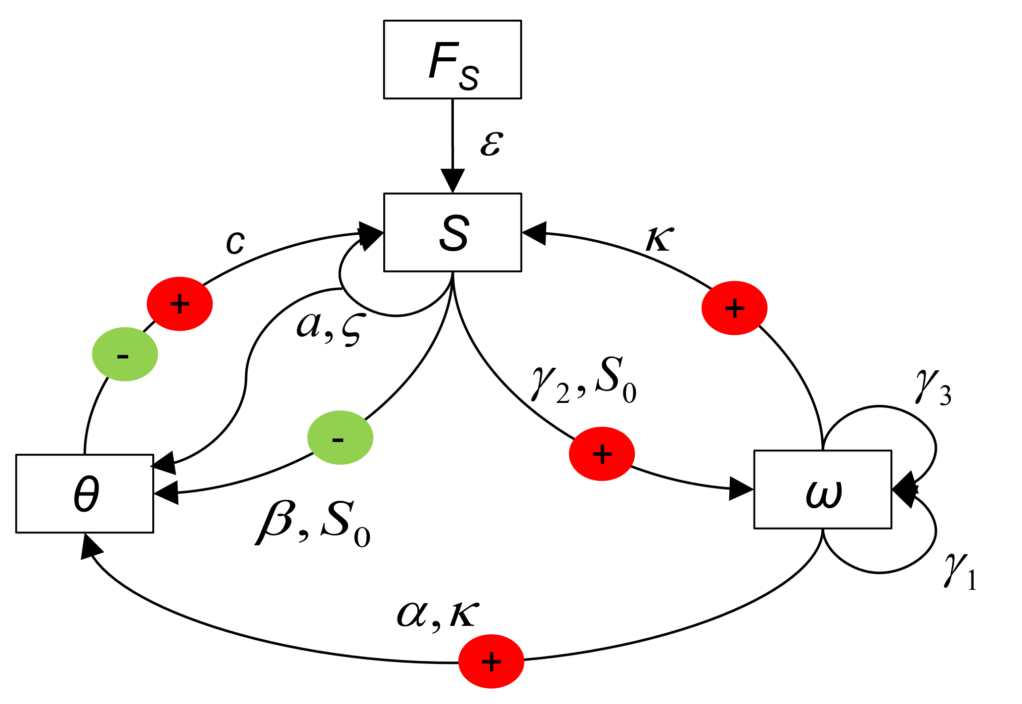
Figure 1Dynamical system connections. Red circles mark positive feedback loops, and green circles mark negative feedback loops.
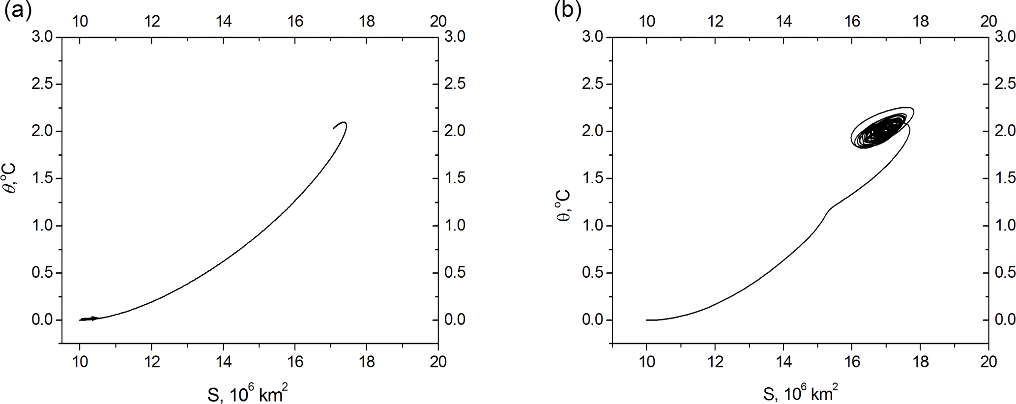
Figure 2System (Eqs. 24–26) evolution without astronomical forcing involved, ε=0 (a); the same with very weak forcing, ε=0.01 (b).
For a steady-state solution in Fig. 2 (panel a) ε=0. To test the stability of the equilibrium point, we repeated calculations with a weak insolation forcing, ε=0.01. The results, presented in Fig. 2 (panel b), show that the equilibrium point is stable.
Initial conditions are
This steady-state solution can be obtained from the system (Eqs. 24–26) if we set all derivatives equal to zero.
Then, for ε=0
Here, 〈S〉, 〈θ〉, and 〈ω〉 are the steady-state solutions of corresponding variables.
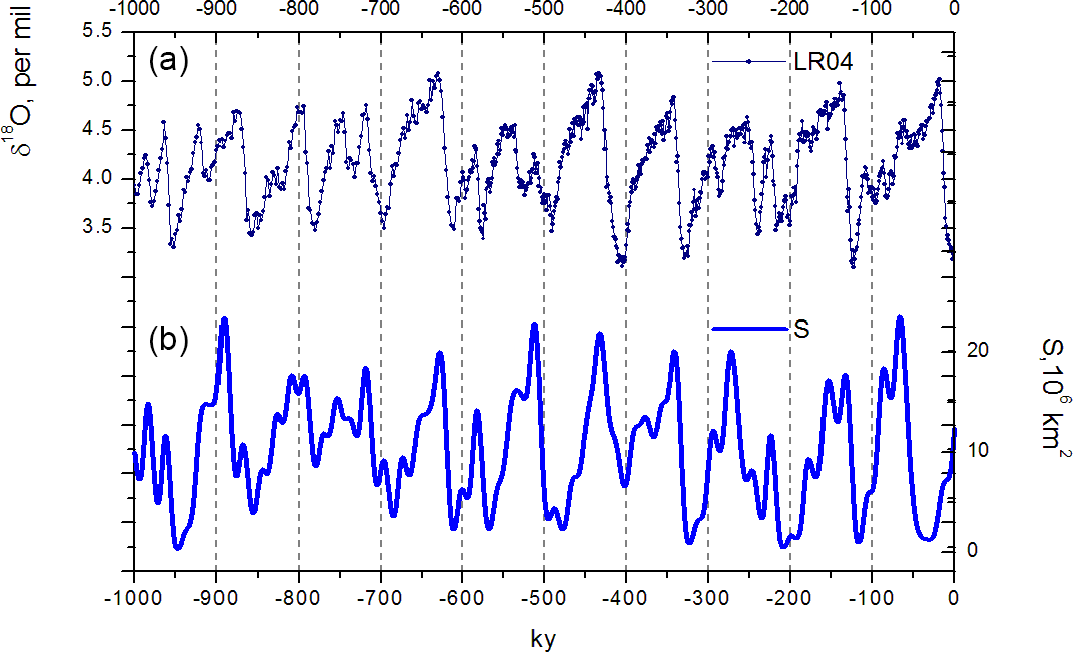
Figure 3Glacial rhythmicity over the past 1 000 000 years: Lisiecki and Raymo (2005) benthic foraminifera δ18O data (a); system-produced (Eqs. 24–26) evolution of glaciation area S (b).
It can be seen that without climate feedbacks involved (, or ), the steady-state extent of glaciation is defined by ice-sheet properties only, . This glaciation extent may be reduced by a climate damping factor ( or enhanced by climate positive feedback (.
We will measure the total climate impact Ω as a difference between the strength of climate positive feedback and a damping factor
and introduce a dimensionless number, V (variability number), as a ratio of the intensity of climate impact Ω on the intensity of ice-sheet own negative feedback:
This number is small if the positive feedback is weak and it is high otherwise. We will now demonstrate that the variability number, V, defines different modes of glacial rhythmicity.
4.2 Mode I: late Pleistocene, V=0.75
We will now present the results of dynamical system evolution for the same set of parameters as in Sect. 4.1 but ε=0.11 km kyr−1. Very similar results have been produced for other sets of parameters as long as ; for example, α=2.1 and κ=0.006 km kyr−1 ∘C−1 (slightly increased positive feedback), β=1.8 ∘C 10−6 km−2) (slightly decreased negative feedback), γ2 and γ3 are proportionally increased by about 10 %, or κ and c are proportionally increased by about 10 %, and so on. In Fig. 3 we show the results of calculations of the glaciation extent for the last 1 000 000 years together with the LR04 benthic foraminifera δ18O stack (Lisiecki and Raymo, 2005).
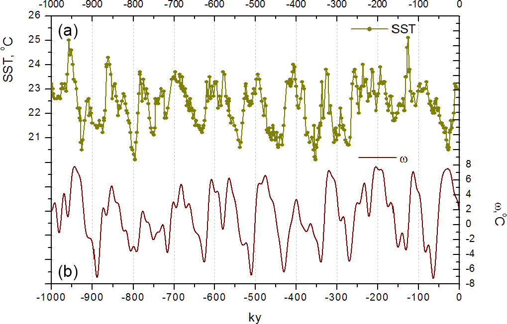
Figure 4Ocean temperature evolution over the past 1 000 000 years: Herbert et al. (2010) data of tropical ocean temperatures (a); system-produced (Eqs. 24–26) evolution of climate temperature changes ω (b).
The major events of the last million years are reproduced reasonably well, except for the interglacial of 400 kyr ago (marine isotopic stage 11), which has usually been described as a long and deep interglacial and obviously the last interglacial starting 30 000 years ago instead of 10 000 years ago, driving the present day into a glaciation. The timing of all other interglacials coincides with Past Interglacial Working Group of PAGES (2016) data. The deglaciation associated with termination V leading to stage 11 creates a difficult problem indeed (see, e.g., Berger and Wefer, 2003). It is remarkable that the model (Eqs. 24–26) actually simulates a deglaciation around 430 ka BP, while the celebrated Imbrie and Imbrie (1980) model, for example, missed it and that termination remains a challenge for a model of intermediate complexity with an interactive carbon cycle such as CLIMBER (Victor Brovkin, personal communication, 2018). Furthermore, the Fig. 3 results illustrate the fact that the termination V was a slower process than other deglaciations, which is reasonably consistent with sea-level reconstructions (Rohling et al., 2010, 2014). However, the simulated sea level during stage 11 is not as high as the observations suggest, and it is possible that the model (Eqs. 24–26), by using mid-June insolation as the forcing metric, is not giving enough weight to obliquity. Some tuning efforts at this point could be exercised to get an even better fit, but we believe that exact replication should not be expected from a simple model like ours taking into account all uncertainties involved in parameters values. It should also be taken into consideration that the V number (and each of the eight parameters involved in its definition) does not have to be a constant as has been implied in this section, but may experience a slow trend. For example, when the V number evolves from its low early Pleistocene value to its higher late Pleistocene value to simulate the mid-Pleistocene transition (see Sect. 4.5 below), the glacial variability, consistent with instrumental records, is at maximum amplitude around 400 kyr ago. The timing of the last glacial cycle for an evolving V number is also close to the LR04 record. It should also be recalled that the benthic curve is not strictly a measure of only ice volume.
Figure 4 compares the modeled climate temperature ω with the reconstruction of tropical ocean temperatures provided by Herbert et al. (2010). It can be noted that calculated temperature changes and ocean temperature data generally evolve in phase, though, like in the case with glaciation extent (Fig. 3), the last interglacial slightly leads the data.
In Fig. 5 we compare spectral diagrams for calculated glaciation volume (ζS5∕4) against LR04 benthic δ18O data and for calculated ω values against Herbert et al. (2010) tropical ocean temperature data. In both cases, the results are reasonably consistent: in all cases periods of nearly 100 kyr clearly dominate. Precession and obliquity periods can be easily distinguished, though in both empirical diagrams 40 kyr periods are more visible than in the model.
The sequence of events that produce 100 kyr periods can be visualized by zooming into a typical cycle. For this purpose, in Fig. 6 we show the evolution of the derivatives of the model variables, together with insolation changes.
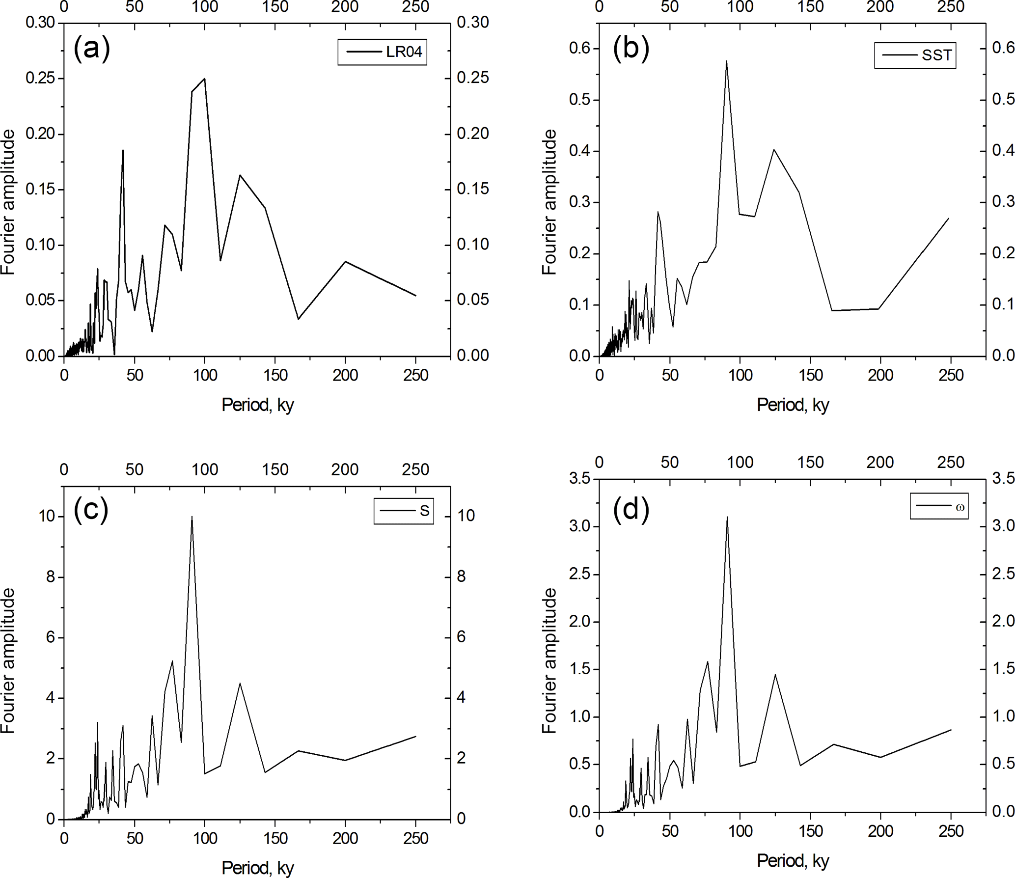
Figure 5Spectral diagrams of LR04 benthic foraminifera δ18O data (a), calculated glaciation volume, ζS5∕4 (c), Herbert et al. (2010) tropical ocean temperature data (b), and calculated ω values (d).
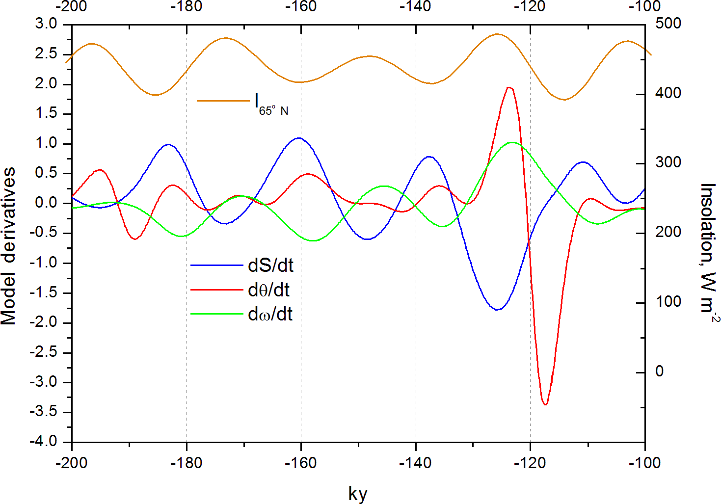
Figure 6Time evolution of model derivatives during one glacial cycle against insolation changes.
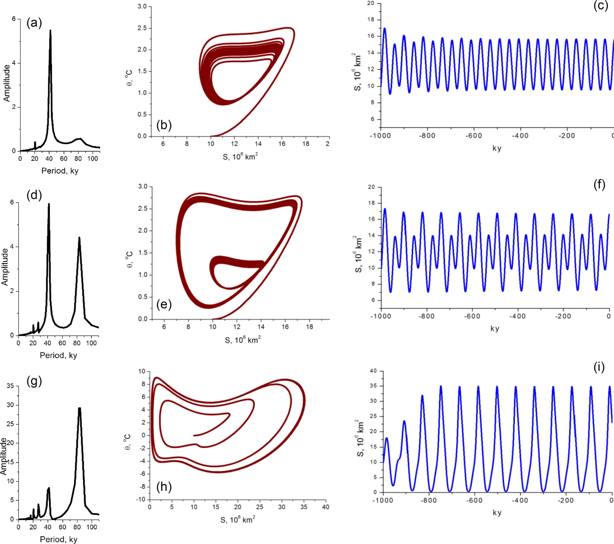
Figure 7Model response to a single obliquity period sinusoid kyr). Panels (a–c) ε=0.07; panels (d–f) ε=0.082; panels (g–i) ε=0.11. (a, d, g) Fourier spectra, (b, e, h) phase diagrams, S (106 km2) vs. θ ∘C, and (c, f, i) time series, S (106 km2). For V=0.75 and a relatively high amplitude of forcing (ε>0.07), the model (Eqs. 24–26) produces fluctuations of a doubled obliquity period.
It can be seen that when ice grows, its basal temperature increases (with a time lag) due to increased internal friction and due to a more prominent role of the geothermal heat flux. As we discussed earlier, it provides a negative feedback to ice-sheet growth. At the same time, climate temperature is getting lower as well, and it creates a positive feedback for ice growth. Four times during this cycle the astronomical forcing (precession) “challenges” ice growth by trying to switch it to the disintegration mode. These attempts fail three times: ice volume is not high enough and positive feedback from the climate acting through its mass balance (κω) and through basal temperature (αω) is not strong enough to counteract ice-sheet own negative feedback (βS). The fourth attempt succeeds. Ice is high enough, positive feedback is strong, and disintegration proceeds until ice almost disappears. This scenario is consistent with the idea that glacial cycles skip insolation cycles until ice has grown to a point that precipitates its full disintegration, as conceptualized among others by Paillard (1998) and Tzedakis et al. (2017). It is to some extent reminiscent of the phase-locking mechanism mathematically analyzed by Tziperman et al. (2006) and Crucifix (2013). In our model, though, the role of insolation is much bigger than in phase-locking scenarios: insolation variations define not only the phase of ice fluctuations but, being nonlinearly amplified, they actually define the period of glacial rhythmicity as well. The mechanism involved in the glacial frequency setting is similar to a “period-two” (period doubling) response to astronomical forcing exhibited by a conceptual model of Daruka and Ditlevsen (2016). To illustrate this “period-two” behavior, we solve our system (Eqs. 24–26) with astronomical forcing replaced by a single obliquity period sinusoid kyr). The results of the calculations, presented in Fig. 7, show that for a relatively high amplitude of forcing (ε>0.07) our model produces fluctuations of a doubled obliquity period. It is interesting that the signatures of such period doubling have been found in LR04 variability (Vakulenko et al., 2011).
Until full dynamical system analysis is performed, which is clearly outside of the scope of this paper, we will (loosely) reference this mechanism as “nonlinear amplification” and we will demonstrate that this mechanism manifests itself differently depending on the V number, which is a measure of the positive-to-negative feedback ratio.
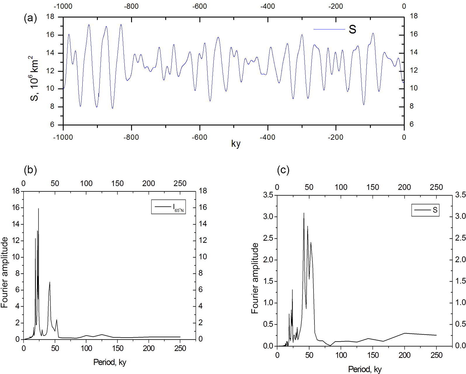
Figure 8Example of variable S (106 km2) evolution for Mode II (a). Spectral diagrams of summer insolation changes at 65∘ N (b) and of calculated glaciation volume, ζS5∕4 (c).
4.3 Mode II: late Pliocene–early Pleistocene, V=0
We will now present the results of dynamical system evolution for the same set of parameters as in Sect. 4.2 but α=0 and κ=0 (or ); i.e., positive feedback is weak, V=0. The results of the calculations are shown in Fig. 8.
The local mid-July insolation at 65∘ N, FS (Berger and Loutre, 1991), is dominated by a precession period of about 23 kyr (Fig. 8b), while the early Pleistocene paleoclimatic data indicate a stronger response in the 40 kyr period band. The integrated summer insolation, which is dominated by the 41 kyr obliquity cycle (Huybers, 2006), is often invoked to explain this discrepancy. It is interesting that our model produces fluctuations with a dominating obliquity period (Fig. 8c) without needing integrated summer forcing. It happens due to period-doubling dynamics, in this case precession periods. To illustrate this phenomenon, we solve our system (Eqs. 24–26) with astronomical forcing replaced by a single precession period sinusoid kyr). The results of the calculations, presented in Fig. 9, show that when V=0 our model produces fluctuations of a doubled precession period.
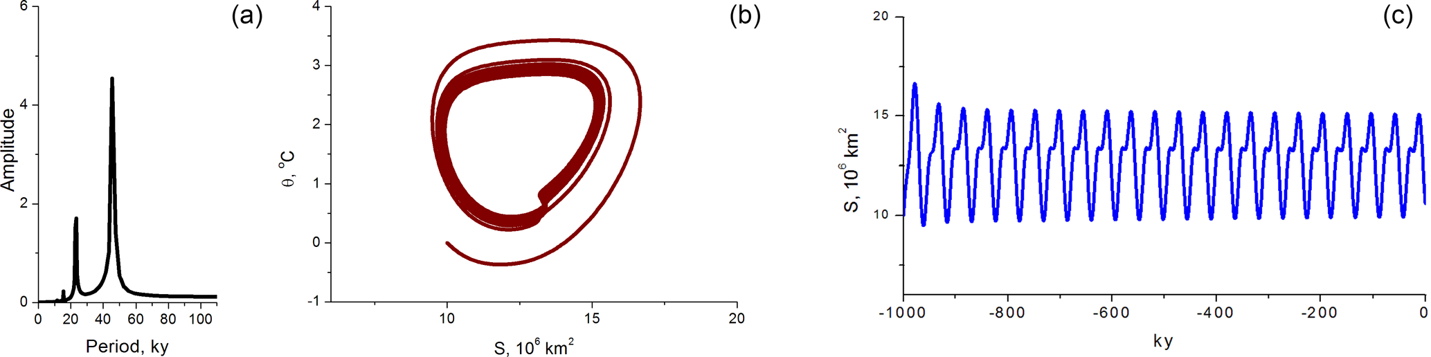
Figure 9Model response to a single precession period sinusoid kyr): for V=0 and ε=0.04 the model (Eqs. 24–26) produces fluctuations of a doubled precession period. (a) Fourier spectra; (b) phase diagram, S (106 km2) vs. θ ∘C; (c) time series, S (106 km2).
If we also set S0=2 (106 km2) we will get fluctuations with a lower mean level of ice-area extension, which may be relevant to early Pleistocene fluctuations (Fig. 10). Astronomical periods are still very visible in the ice spectral diagram of ice fluctuations.
4.4 Mode III: strong ocean feedback, V→1
In this section we show that the system would produce fluctuations of about 400 kyr if the positive feedback increased further (V→1). Specifically, we present the results of dynamical system evolution (Fig. 11) for the same set of parameters as in Sect. 4.2 but β=1.57 ∘C 10−6 km−2), i.e., V=0.94. Very similar results have been produced for different sets of parameters as long as V∼0.95; for example, γ2=0.26 ∘C 10−6 km−2 kyr−1.

Figure 10Example of variable S (106 km2) evolution for Mode II (a). S0=2 (106 km2). Spectral diagrams of summer insolation changes at 65∘ N (b) and of calculated glaciation volume, ζS5∕4 (c).
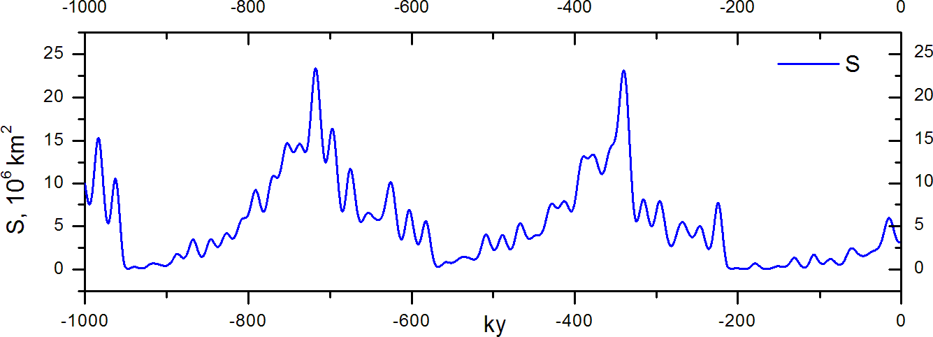
The results may seem to be counterintuitive at first because one would expect faster ice growth as the positive feedback increases. However, it makes sense by observing that with stronger positive feedback every astronomical “challenge” is more successful in retreating ice. Consequently, it takes longer to grow ice to the level at which its retreat can be really strong. The ratio between positive and negative feedbacks determines how long it takes for ice to grow until a level at which it is vulnerable to the astronomical “challenge” (in our model it corresponds roughly to km2). This example also shows that if the ratio between positive and negative feedbacks were wrong (i.e., the wrong V number), then the astronomical forcing would in no case reproduce the correct sequence of events. In other words, incorrect physics cannot be rescued by tuning the strength of the astronomical forcing.

Figure 12Glacial rhythmicity over the past 3 000 000 years: Lisiecki and Raymo (2005) benthic foraminifera δ18O data; system-produced (Eqs. 24–26) evolution of glaciation area S (106 km2).
4.5 Mode II–Mode I transition (mid-Pleisctocene transition)
If we attribute the V=0 mode to the early Pleistocene and the V=0.75 mode to the late Pleistocene, then the V number may provide some guidance about possible scenarios to explain the mid-Pleistocene transition. Since the V number is a combination of multiple parameters, it implies that multiple scenarios are possible. For memory, , where the parameters β, c, and S0 are glaciation parameters, α and κ are parameters associated with atmospheric circulations, and γ1, γ2, and γ3 are ocean parameters. Slow variations in atmospheric, ocean, or even glaciation parameters (Clark and Pollard, 1998) are quite possible. It is outside of the scope of this paper to provide a full list of possible scenarios, but at least one plausible suggestion can be made. A commonly invoked scenario involves tectonic forcing, including volcanism and weathering processes, which could produce long-term variations in carbon dioxide such that it dropped from above 300 ppm during the early Pleistocene to its current values of about 250 ppm. The scenario remains commonly invoked (Saltzman and Maasch, 1991; Saltzman and Verbitsky, 1993a, b; Raymo, 1997; Paillard and Parrenin, 2004) even though it is fair to admit that the observations remain uncertain (Zhang et al., 2013) and that this scenario has been challenged (Honisch et al., 2009). Whether or not this specific mechanism is responsible for the regime change, it still seems reasonable to assume that the slow trend in climatic condition occurred and that it can cause a drift in the climate positive feedback (e.g., γ2), specifically an increase from lower to higher values. As an illustration, in Figs. 12–14 we present an example of such a transition. In this instance, at kyr, γ2, S0, and ε have been reduced by 60 % from their Mode I values and then increased linearly so that they regained 100 % of their Mode I values at present (t=0). A forced change in the glaciation reference line S0 defines a gradual increase in the global ice volume; changes in the sensitivity parameter ε cause an increase in fluctuation amplitudes. The most dramatic change, i.e., the transition from about 40 kyr period fluctuations to predominantly 100 kyr period fluctuations, is due to the intensified climate positive feedback , γ2, which caused a gradual increase in the V number from V=0.3 at kyr to V=0.75 at present (t=0). The example shows reasonable consistency between model results and the data: in model calculations and in the records of instrumental measurements (Fig. 13), the early Pleistocene is dominated by mostly 40 kyr fluctuations. At about 1.5–1.3 Myr ago, 100 kyr rhythmicity becomes predominant. Its amplitude is at a maximum about 400 kyr ago in both instrumental and model time series. The evolution of the cross-wavelet spectrum (Grinsted et al., 2004) between benthic foraminifera δ18O data and the system-produced (Eqs. 24–26) evolution of glaciation area S (Fig. 14) shows a mostly in-phase relationship between the model and measurement records on 40 and 100 kyr periods.
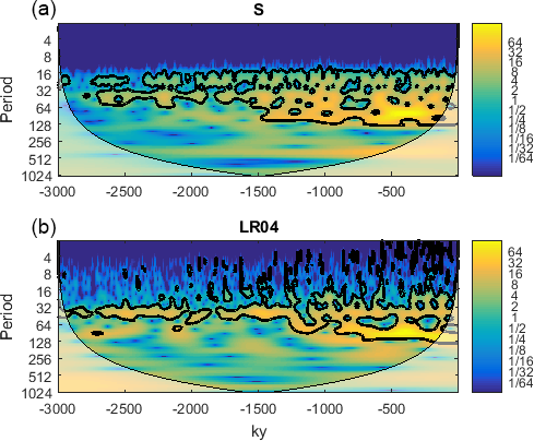
Figure 13Evolution of wavelet spectra over the past 3 000 000 years. System-produced (Eqs. 24–26) evolution of glaciation area S (106 km2) (a); Lisiecki and Raymo (2005) LR04 benthic foraminifera δ18O data (b). The color scale shows wavelet amplitude, the thick line indicates the peaks with 95 % confidence, and the shaded area indicates the cone of influence for wavelet transform.
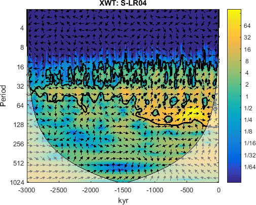
Figure 14Evolution of cross-wavelet spectrum (Grinsted et al., 2004) between Lisiecki and Raymo (2005) benthic foraminifera δ18O data and system-produced (Eqs. 24–26) evolution of glaciation area S. Higher cross-wavelet power (color bar scale) shows areas with high common power wavelet spectra, and the thick contour shows 95 % significance of maxima against red noise. The phase relationship is shown with arrows, whereby an “in-phase” relation is indicated by arrows directed to the right and “antiphase” by arrows directed to the left.
4.6 Role of the Antarctic ice sheet
The system (Eqs. 24–26) can be expanded to include Southern Hemisphere (Antarctic) ice dynamics:
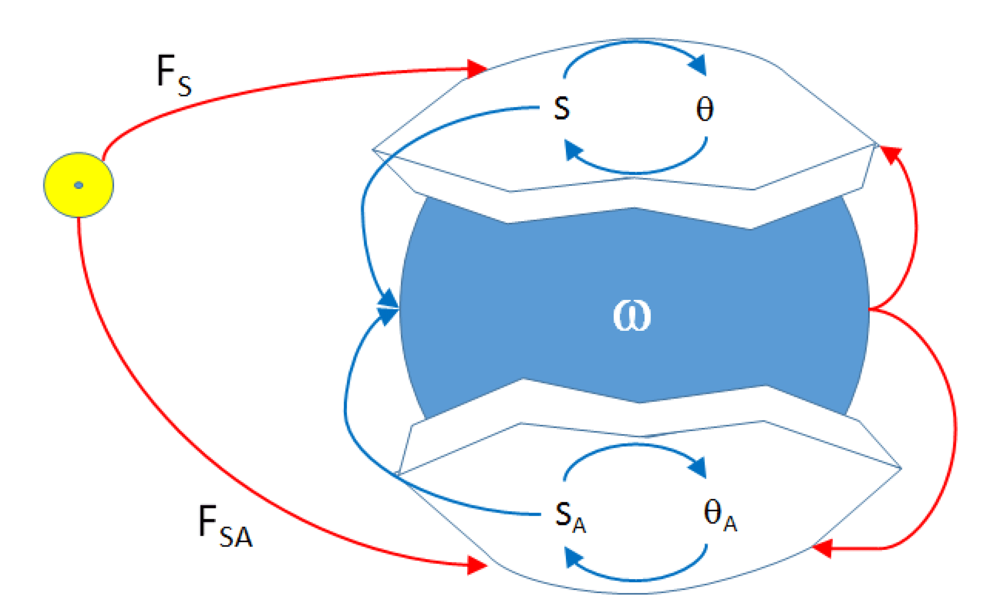
Here, Eqs. (34) and (35) are identical to Eqs. (24) and (25). Equations (37) and (38) describe the evolution of the glaciation area of the Antarctic ice-sheet SA and its basal temperature θA; FSA is mid-January insolation at 65∘ S (Berger and Loutre, 1991); is the area of the Antarctic continent; aA is the rate of snow precipitation and cA is the intensity of basal sliding for the Antarctic ice sheet. All other parameters in Eqs. (37) and (38) are intentionally left the same as in Eqs. (34) and (35), following the assumption that the Antarctic ice sheet and Northern Hemisphere ice sheets are governed by the same physics. Equation (36) is the same as Eq. (26) except that it includes an additional term to reflect a potential control by the Antarctic ice sheet and associated ice shelves (). The system (Eqs. 34–38) is represented graphically in Fig. 15.
The system (Eqs. 34–38) has been solved for the same set of parameters as in Sect. 4.1 but aA=0.5 km ky−1 and cA=0.01 km ky−1 ∘C−1 (implying more positive mass balance of the Antarctic ice sheet than Northern Hemisphere ice sheets). For this set of parameters = const and the system (Eqs. 34–38) takes the following shape:
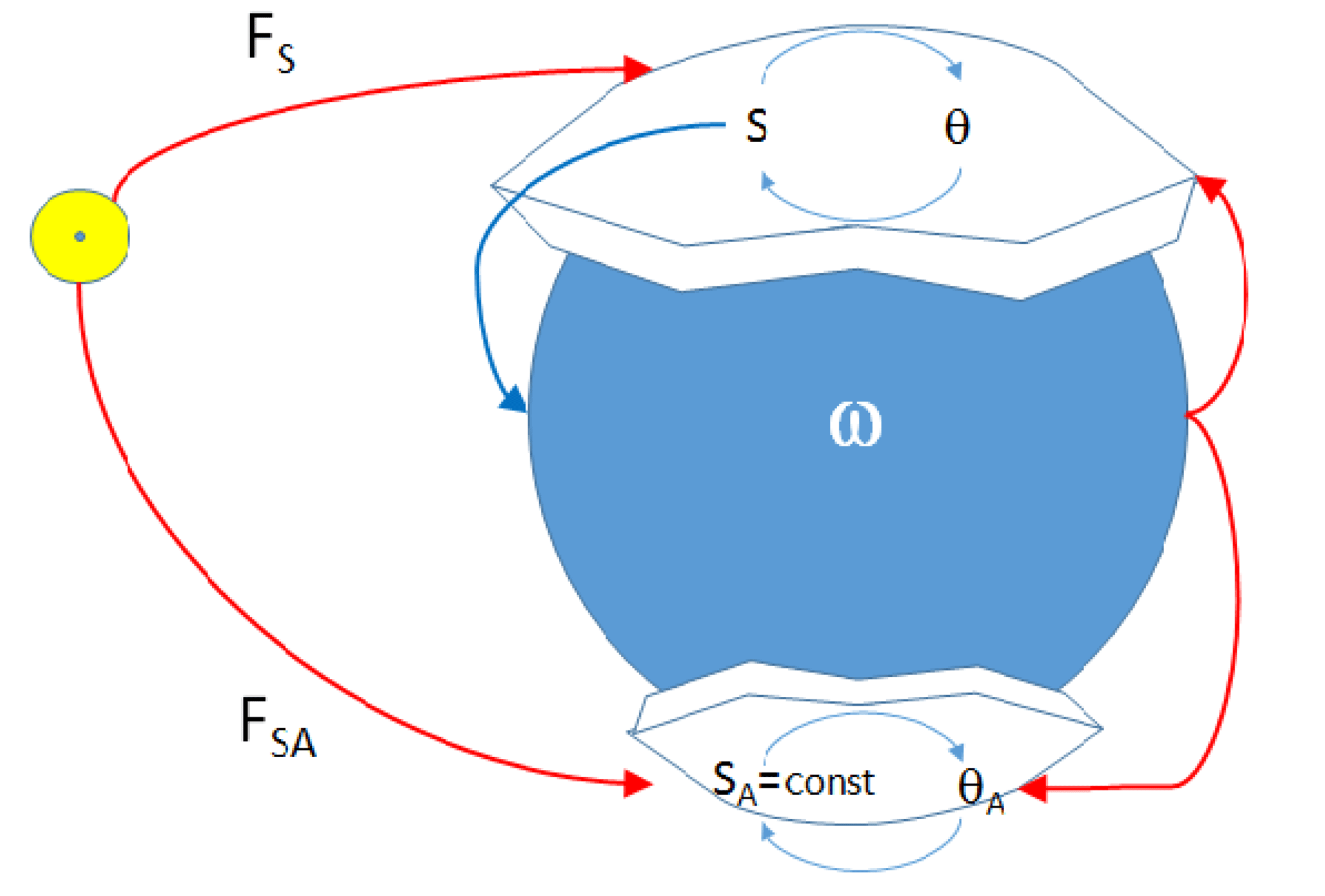
Now, Eqs. (39)–(41) are exactly the same as in our original system (Eqs. 24–26). It means that all previous calculations were conducted with the assumption that the area of Antarctic glaciation remains constant. Interestingly, the system (Eqs. 39–43) has a “diode-like” structure (Fig. 16): Northern Hemisphere insolation has an important impact on Northern Hemisphere glaciation, the extent of glaciation effects on climate temperature, and climate temperature effects on Antarctic mass balance, surface temperature, and eventually ice-sheet basal temperature.
But since = const, there is no “opportunity” for Southern Hemisphere insolation to be amplified by climate positive feedback and to propagate its signal north. This produces a simple explanation for the synchronous response of the Northern and Southern Hemisphere to Northern Hemisphere insolation variations.
In this research, we build the theory of Pleistocene ice ages without a prior assumption about internal climate system instability. For this purpose, we derived a simple model of the global climate system using scaled equations of ice-sheet thermodynamics to combine them with a linear equation describing changes in climate temperature. The model obtained is a nonlinear dynamical system incorporating three variables: area of glaciation, ice-sheet basal temperature, and characteristic temperature of outside-of-glacier climate. Without astronomical forcing, the system evolves to equilibrium. When it is astronomically forced, depending on the values of the parameters involved, the system is capable of producing different modes of rhythmicity, some of which are consistent with paleoclimate records of the early and late Pleistocene.
Three mechanisms captured by our model are of primary importance. The first one is a nonlinear dependence of the intensity of ice discharge on ice-sheet dimensions: dS∕d. This nonlinearity was postulated by Huybers (2009) as being proportional to ice volume in the ninth degree; here, we were able to quantify it using the fundamentals of ice flow revealed by Eq. (5). The second mechanism is basal sliding intensity. Its importance was expressed by MacAyeal (1993), Payne (1995), and Marshall and Clark (2002) for the Laurentide ice sheet. In this paper, using the scaling of ice thermodynamics, we were able to connect sliding intensity to climatic factors. When internal ice-sheet dynamics are coupled with the rest of the climate system via a linear climate temperature equation, the above two phenomena jointly form a third one: the nonlinear amplification of the insolation forcing. This amplification defines not only the phase but also the period of glacial rhythmicity by producing multi-obliquity and multi-precession periods similar to a conceptual model of Daruka and Ditlevsen (2016). We determined that this mechanism manifests itself differently depending on a specific balance between positive and negative feedbacks in the system.
To measure this balance, we introduced a dimensionless variability number or the V number as the ratio between the intensities of glaciation and climate feedbacks. When the climate positive feedback is weak (V∼0), the system exhibits fluctuations with a dominating period of about 40 kyr, which is in fact a combination of a doubled precession period and (to smaller extent) obliquity period. When the positive feedback increases (V∼0.75), the system evolves with a roughly 100 kyr period, which is a doubled obliquity period. Finally, when the positive feedback increases further (V∼0.95), the system produces fluctuations of about 400 kyr. When the V number is gradually increased from its low early Pleistocene values to its late Pleistocene value of V=0.75, the system reproduces the mid-Pleistocene transition: while the early Pleistocene is dominated by mostly 40 kyr fluctuations, at about 1.5 Myr ago the 100 kyr period rhythmicity emerges and finally dominates.
Thus, our theory is capable of explaining all major features of the Pleistocene climate benthic isotopic record, including the mostly 40 kyr fluctuations of the early Pleistocene, a transition from a 40 kyr nonlinear regime to a 100 kyr nonlinear regime, and the 100 kyr fluctuations of the late Pleistocene.
The crucial role of climate feedback is evident in the Southern Hemisphere as well. The Antarctic ice-sheet area of glaciation is limited by the Antarctic continent and therefore it cannot engage in a strong positive feedback from the rest of the climate system. At the same time, the impact of the Northern Hemisphere is amplified by climate positive feedback and affects Antarctica. This asymmetry may provide an explanation for the synchronous response of the Northern and Southern Hemisphere to Northern Hemisphere insolation variations.
The system we described in this paper has 11 parameters, but all of them are at least partly constrained. Some of them are based on empirical data of present ice sheets and others can be calibrated with a three-dimensional ice-sheet model and global general circulation climate models. Most revealing, though, as we discussed above, is the V number, a dimensionless combination of eight parameters. Given that the V number is dimensionless, this model could be used to investigate other physics that may be involved in producing ice ages. In such a case, the equation currently representing the characteristic temperature of outside-of-glacier climate would describe some other climate component of interest, like the marine or terrestrial carbon cycle or dust transport. As long as this component is capable of producing an appropriate V number, it may be considered an acceptable candidate. However, we have not found it necessary to assume a priori a nonlinearity in the equations governing climate or carbon cycle dynamics to explain ice-age cycles as they appear in the benthic isotopic record.
Model code and data files are available at https://github.com/DmitryVolobuev1973/Model-of-Pleistocene-Glacial-Cycles (Verbitsky et al., 2018).
To test the response of ice-sheet basal temperature to climatic factors such as precipitation rate, air temperature, and ice-sheet area, four numerical experiments have been conducted with a 3-D ice-sheet model applied to Antarctica:
- a.
current climate: d, dT=0, d;
- b.
increased (doubled) precipitation: d, dT=0, d;
- c.
increased temperature (with unavoidable retreat of the ice sheet): d, dT=10C, d; and
- d.
increased precipitation and increased temperature: d, dT=10C, d.
The ice-sheet–shelf model used here is described in detail in Pollard and DeConto (2012a) and additionally in Pollard et al. (2015) and DeConto and Pollard (2016). It uses a hybrid combination of shallow ice approximation and shallow shelf approximation (SIA–SSA) dynamics, which consider vertical shearing (SIA) and horizontal stretching (SSA) while neglecting higher-order modes of flow. A flux condition at the grounding line (Schoof, 2007) is imposed that allows for reasonable grounding-line migration without very fine resolution in the grounding zone. These approximations yield satisfactory results in long-term large-scale intercomparisons vs. higher-order models (Pattyn et al., 2012, 2013). The distribution of basal sliding coefficients under modern grounded regions is determined from a previous inverse run fitting to modern ice thicknesses (Pollard and DeConto, 2012b). There is no explicit basal hydrology; basal sliding is allowed only if the base is at or close to the melt point. All experiments here are run on a polar stereographic grid with 20 km grid resolution.
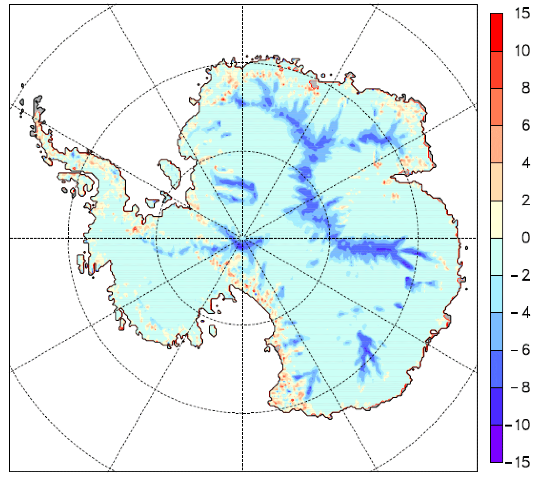
Figure A1Basal ice temperature change (K) for experiment B minus the control experiment A. These are absolute temperature changes, not relative to the pressure melt point.
Atmospheric climate forcing is obtained from a modern Antarctic climatological dataset (ALBMAP; Le Brocq et al., 2010). Monthly mean air temperatures and precipitation are interpolated to the ice-sheet grid and lapse rate corrected to the ice surface elevation (Pollard and DeConto, 2012a); a simple model is used to estimate net surface mass balance using positive-degree-day melting and refreezing. Oceanic melting below floating ice shelves depends on the 400 m water temperature at the nearest grid cell in a modern oceanographic dataset (Levitus et al., 2012).
The experiments are initialized to the modern Antarctic state (Bedmap2; Fretwell et al., 2013). All experiments are run with invariant climate forcing for 100 000 years to ensure that the ice sheet is very nearly equilibrated. The standard physical ice-sheet model is used, except that grounding-line locations and ice-shelf distributions are held fixed to modern (as in Pollard and DeConto, 2012b) to avoid grounding-line advance in marine sectors that would complicate interpretation of the results. For experiment A (current climate control), modern climate forcing is used as described above. For experiment B, prescribed precipitation rates are doubled everywhere. For experiment C, a uniform increment of +10 ∘C is added to all prescribed atmospheric temperatures. For experiment D, the modifications for B and C are combined. In all experiments, the lapse rate adjustment to precipitation rates is disabled to ensure that precipitation rates in experiments B and D are exactly double those in A and C.
The results of the experiments are shown in Figs. A1–A3 in which we show basal temperature changes relative to the present climate. Table A1 presents integrated results. As seen in Table A1, the sign and order of magnitude of the basal temperature response to climatic forcing predicted by our scaling estimates are consistent with the results of the 3-D ice-sheet model.
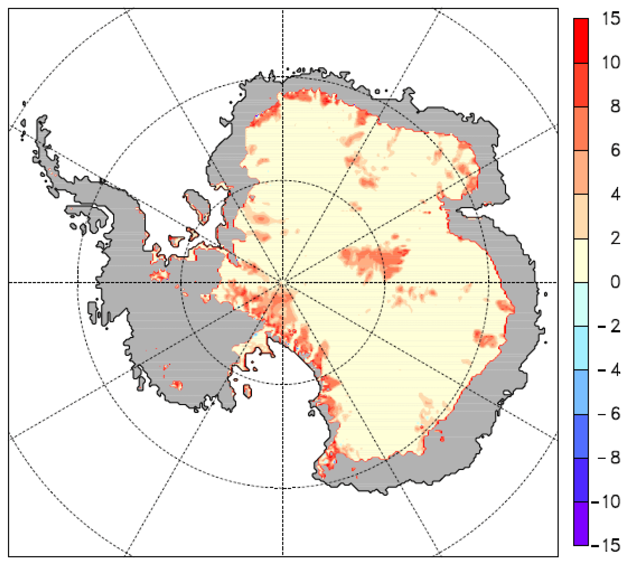
Figure A2Basal ice temperature change (K) for experiment C minus the control experiment A (absolute temperature changes, not relative to the pressure melt point).
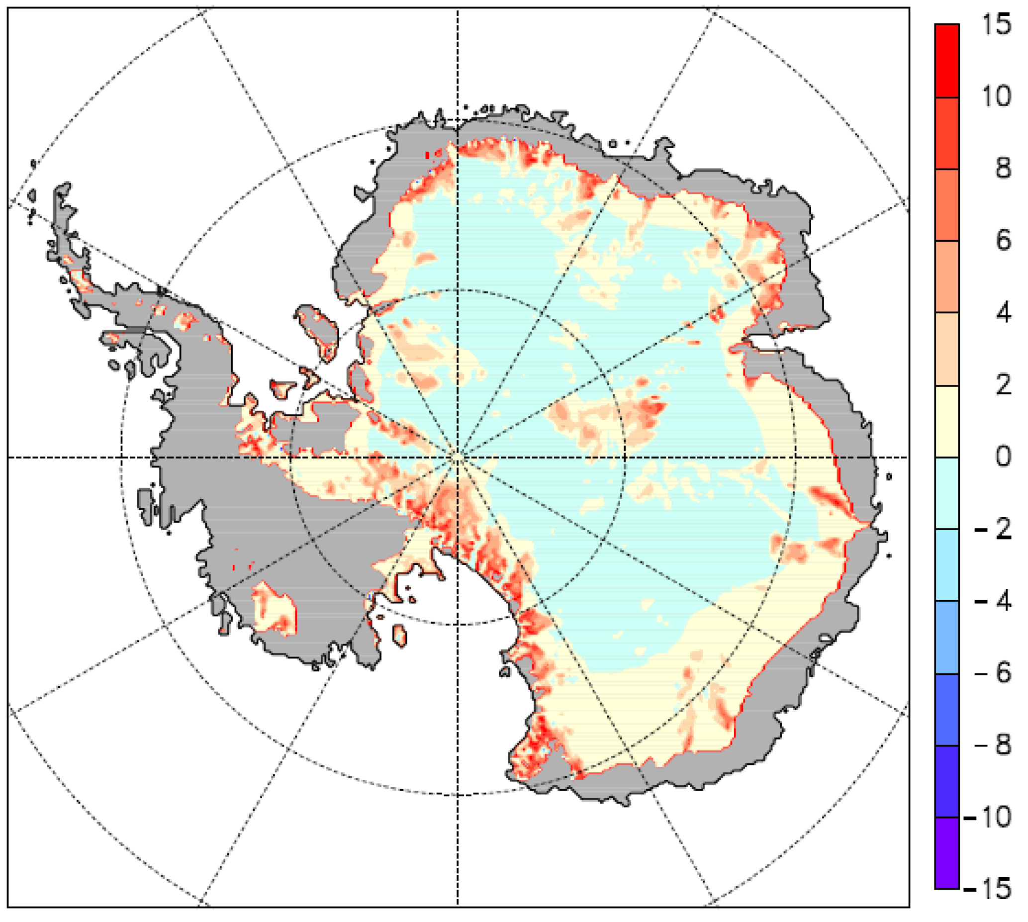
Figure A3Basal ice temperature change (K) for experiment D minus the control experiment A (absolute temperature changes, not relative to the pressure melt point).
Table A1Basal temperature changes relative to the present climate (∘C).
MV conceived the research and developed the model. MV, MC, and DV contributed equally to the design of the research and to writing the paper. DV digitized the model.
The authors declare that they have no conflict of interest.
We are grateful to David Pollard for providing the Appendix, which contains the results of numerical experiments
with a three-dimensional Antarctic ice-sheet model.
Edited by: Gerrit Lohmann
Reviewed by: two anonymous referees
Abe-Ouchi, A., Saito, F., Kawamura, K., Raymo, M. E., Okuno, J. I., Takahashi, K., and Blatter, H.: Insolation-driven 100,000-year glacial cycles and hysteresis of ice-sheet volume, Nature, 500, 190–194, 2013.
Ashkenazy, Y. and Tziperman, E.: Are the 41 kyr glacial oscillations a linear response to Milankovitch forcing?, Quaternary Sci. Rev., 23, 1879–1890, 2004.
Ashwin, P. and Ditlevsen, P.: The middle Pleistocene transition as a generic bifurcation on a slow manifold, Clim. Dynam., 45, 2683–2695, https://doi.org/10.1007/s00382-015-2501-9, 2015.
Berger, A. and Loutre, M. F.: Insolation values for the climate of the last 10 million years, Quaternary Sci. Rev., 10, 297–317, 1991.
Berger, W. H. and Wefer, G.: On the Dynamics of the Ice Ages: Stage-11 Paradox, Mid-Brunhes Climate Shift, and 100-Ky Cycle, in: Earth's Climate and Orbital Eccentricity: The Marine Isotope Stage 11 Question, Geophysical Monograph-American Geophysical Union, Washington, DC, 41–59, 2003.
Chalikov, D. V. and Verbitsky, M. Y.: Modeling the Pleistocene ice ages, Adv. Geophys., 32, 75–131, 1990.
Clark, P. U. and Pollard, D.: Origin of the middle Pleistocene transition by ice sheet erosion of regolith, Paleoceanography, 13, 1–9, 1998.
Clark, P. U., Archer, D., Pollard, D., Blum, J. D., Rial, J. A., Brovkin, V., Mix, A. C., Pisias, N. G., and Roy, M.: The middle Pleistocene transition: characteristics, mechanisms, and implications for long-term changes in atmospheric pCO2, Quaternary Sci. Rev., 25, 3150–3184, 2006.
Crucifix, M.: Why could ice ages be unpredictable?, Clim. Past, 9, 2253–2267, https://doi.org/10.5194/cp-9-2253-2013, 2013.
Daruka, I. and Ditlevsen, P.: A conceptual model for glacial cycles and the middle Pleistocene transition, Clim. Dynam., 46, 29–40, https://doi.org/10.1007/s00382-015-2564-7, 2016.
DeConto, R. M. and Pollard, D.: Contribution of Antarctica to past and future sea-level rise, Nature, 531, 591–597, 2016.
Ellis, R. and Palmer, M.: Modulation of ice ages via precession and dust-albedo feedbacks, Geosci. Front., 7, 891–909, 2016.
Fretwell, P., Pritchard, H. D., Vaughan, D. G., Bamber, J. L., Barrand, N. E., Bell, R., Bianchi, C., Bingham, R. G., Blankenship, D. D., Casassa, G., Catania, G., Callens, D., Conway, H., Cook, A. J., Corr, H. F. J., Damaske, D., Damm, V., Ferraccioli, F., Forsberg, R., Fujita, S., Gim, Y., Gogineni, P., Griggs, J. A., Hindmarsh, R. C. A., Holmlund, P., Holt, J. W., Jacobel, R. W., Jenkins, A., Jokat, W., Jordan, T., King, E. C., Kohler, J., Krabill, W., Riger-Kusk, M., Langley, K. A., Leitchenkov, G., Leuschen, C., Luyendyk, B. P., Matsuoka, K., Mouginot, J., Nitsche, F. O., Nogi, Y., Nost, O. A., Popov, S. V., Rignot, E., Rippin, D. M., Rivera, A., Roberts, J., Ross, N., Siegert, M. J., Smith, A. M., Steinhage, D., Studinger, M., Sun, B., Tinto, B. K., Welch, B. C., Wilson, D., Young, D. A., Xiangbin, C., and Zirizzotti, A.: Bedmap2: improved ice bed, surface and thickness datasets for Antarctica, The Cryosphere, 7, 375–393, https://doi.org/10.5194/tc-7-375-2013, 2013.
Ganopolski, A. and Roche, D. M.: On the nature of lead–lag relationships during glacial–interglacial climate transitions, Quaternary Sci. Rev., 28, 3361–3378, https://doi.org/10.1016/j.quascirev.2009.09.019, 2009.
Ganopolski, A., Calov, R., and Claussen, M.: Simulation of the last glacial cycle with a coupled climate ice-sheet model of intermediate complexity, Clim. Past, 6, 229–244, https://doi.org/10.5194/cp-6-229-2010, 2010.
Grinsted, A., Moore, J. C., and Jevrejeva, S.: Application of the cross wavelet transform and wavelet coherence to geophysical time series, Nonlin. Processes Geophys., 11, 561–566, https://doi.org/10.5194/npg-11-561-2004, 2004.
Herbert, T. D., Peterson, L. C., Lawrence, K. T., and Liu, Z.: Tropical ocean temperatures over the past 3.5 million years, Science, 328, 1530–1534, 2010.
Honisch B., Hemming, N. G., Archer, D., Siddall, M. and McManus, J. F.: Atmospheric Carbon Dioxide Concentration Across the Mid-Pleistocene Transition, Science, 324, 1551–1554, https://doi.org/10.1126/science.1171477, 2009.
Huybers, P.: Early Pleistocene glacial cycles and the integrated summer insolation forcing, Science, 313, 508–511, 2006.
Huybers, P.: Pleistocene glacial variability as a chaotic response to obliquity forcing, Clim. Past, 5, 481–488, https://doi.org/10.5194/cp-5-481-2009, 2009.
Imbrie, J. and Imbrie, J. Z.: Modeling the climatic response to orbital variations, Science, 207, 943–953, 1980.
Imbrie, J. Z., Imbrie-Moore, A., and Lisiecki, L. E.: A phase-space model for Pleistocene ice volume, Earth Planet. Sc. Lett., 307, 94–102, 2011.
Le Brocq, A. M., Payne, A. J., and Vieli, A.: An improved Antarctic dataset for high resolution numerical ice sheet models (ALBMAP v1), Earth Syst. Sci. Data, 2, 247–260, https://doi.org/10.5194/essd-2-247-2010, 2010.
Levitus, S., Antonov, J. I., Boyer, T. P., Baranova, O. K., Garcia, H. E., Locarnini, R. A., Mishonov, A. V., Reagan, J. R., Seidov, D., Yarosh, E. S., and Zweng, M. M.: World ocean heat content and thermosteric sea level change (0–2000 m), 1955–2010, Geophys. Res. Lett., 39, L10603, https://doi.org/10.1029/2012GL051106, 2012.
Lisiecki, L. E. and Raymo, M. E.: A Pliocene-Pleistocene stack of 57 globally distributed benthic δ18O records, Paleoceanography, 20, PA1003, https://doi.org/10.1029/2004PA001071, 2005.
MacAyeal, D. R.: Binge/purge oscillations of the Laurentide ice sheet as a cause of the North Atlantic's Heinrich events, Paleoceanography, 8, 775–784, 1993.
Marshall, S. J. and Clark, P. U.: Basal temperature evolution of North American ice sheets and implications for the 100 kyr cycle, Geophys. Res. Lett., 29, 2214, https://doi.org/10.1029/2002GL015192, 2002.
Mitsui, T. and Aihara, K.: Dynamics between order and chaos in conceptual models of glacial cycles, Clim. Dynam., 42, 3087–3099, 2014.
Omta, A. W., Kooi, B. W., Voorn, G. A. K., Rickaby, R. E. M., and Follows, M. J.: Inherent characteristics of sawtooth cycles can explain different glacial periodicities, Clim. Dynam., 46, 557–569, https://doi.org/10.1007/s00382-015-2598-x, 2016.
Paillard, D.: The timing of Pleistocene glaciations from a simple multiple-state climate model, Nature, 391, 378–381, https://doi.org/10.1038/34891, 1998.
Paillard, D.: Quaternary glaciations: from observations to theories, Quaternary Sci. Rev., 107, 11–24, https://doi.org/10.1016/j.quascirev.2014.10.002, 2015.
Paillard, D. and Parrenin, F.: The Antarctic ice sheet and the triggering of deglaciations, Earth Planet. Sc. Lett., 227, 263–271, 2004.
Past Interglacial Working Group of PAGES: Interglacials of the last 800,000 years, Rev. Geophys., 54, 162–219, 2016.
Paterson, W. S. B.: The physics of glaciers, Pergamon Press, Oxford, 1981.
Pattyn, F., Schoof, C., Perichon, L., Hindmarsh, R. C. A., Bueler, E., de Fleurian, B., Durand, G., Gagliardini, O., Gladstone, R., Goldberg, D., Gudmundsson, G. H., Huybrechts, P., Lee, V., Nick, F. M., Payne, A. J., Pollard, D., Rybak, O., Saito, F., and Vieli, A.: Results of the Marine Ice Sheet Model Intercomparison Project, MISMIP, The Cryosphere, 6, 573–588, https://doi.org/10.5194/tc-6-573-2012, 2012.
Pattyn, F., Perichon, L., Durand, G., Favier, L., Gagliardini, O., Hindmarsh, R. C. A., Zwinger, T., Albrecht, T., Cornford, S., Docquier, D., Fürst, J. J., Goldberg, D., Gudmundsson, G. H., Humbert, A., Hütten, M., Huybrechts, P., Jouvet, G., Kleiner, T., Larour, E., Martin, D., Morlighem, M., Payne, A. J., Pollard, D., Rückamp, M., Rybak, O., Seroussi, H., Thoma, M., and Wilkens, N.: Grounding-line migration in plan-view marine ice-sheet models: results of the ice2sea MISMIP3d intercomparison, J. Glaciol., 59, 410–422, 2013.
Payne, A. J.: Limit cycles in the basal thermal regime of ice sheets, J. Geophys. Res.-Solid Ea., 100, 4249–4263, 1995.
Pollard, D. and DeConto, R. M.: Description of a hybrid ice sheet-shelf model, and application to Antarctica, Geosci. Model Dev., 5, 1273–1295, https://doi.org/10.5194/gmd-5-1273-2012, 2012a.
Pollard, D. and DeConto, R. M.: A simple inverse method for the distribution of basal sliding coefficients under ice sheets, applied to Antarctica, The Cryosphere, 6, 953–971, https://doi.org/10.5194/tc-6-953-2012, 2012b.
Pollard, D., DeConto, R. M., and Alley, R. B.: Potential Antarctic Ice Sheet retreat driven by hydrofracturing and ice cliff failure, Earth Planet. Sc. Lett., 412, 112–121, 2015.
Raymo, M.: The timing of major climate terminations, Paleoceanography, 12, 577–585, https://doi.org/10.1029/97PA01169, 1997.
Rohling, E. J., Braun, K., Grant, K., Kucera, M., Roberts, A. P., Siddall, M., and Trommer, G.: Comparison between Holocene and Marine Isotope Stage-11 sea-level histories, Earth Planet. Sc. Lett., 291, 97–105, https://doi.org/10.1016/j.epsl.2009.12.054, 2010.
Rohling, E. J., Foster, G. L., Grant, K. M., Marino, G., Roberts, A. P., Tamisiea, M. E., and Williams, F.: Sea-level and deep-sea-temperature variability over the past 5.3 million years, Nature, 508, 477–482, https://doi.org/10.1038/nature13230, 2014.
Ruddiman, W. F.: Ice-driven CO2 feedback on ice volume, Clim. Past, 2, 43–55, https://doi.org/10.5194/cp-2-43-2006, 2006.
Saltzman, B.: Dynamical paleoclimatology: generalized theory of global climate change, in: Vol. 80, Academic Press, San Diego, CA, 2002.
Saltzman, B. and Maasch, K. A.: A first-order global model of late Cenozoic climatic change II. Further analysis based on a simplification of CO2 dynamics, Clim. Dynam., 5, 201–210, 1991.
Saltzman, B. and Verbitsky, M. Y.: Asthenospheric ice-load effects in a global dynamical-system model of the Pleistocene climate, Clim. Dynam., 8, 1–11, 1992.
Saltzman, B. and Verbitsky, M. Y.: Multiple instabilities and modes of glacial rhythmicity in the Plio-Pleistocene: a general theory of late Cenozoic climatic change, Clim. Dynam., 9, 1–15, 1993a.
Saltzman, B. and Verbitsky, M. Y.: The late Cenozoic glacial regimes as a combined response to earth-orbital variations and forced and free CO2 variations, in: Ice in the Climate System, Springer-Verlag, Berlin, Heidelberg, 343–361, 1993b.
Saltzman, B. and Verbitsky, M.: Late Pleistocene climatic trajectory in the phase space of global ice, ocean state, and CO2: Observations and theory, Paleoceanography, 9, 767–779, 1994a.
Saltzman, B. and Verbitsky, M.: CO2 and glacial cycles, Nature, 367, 419–419, 1994b.
Schoof, C.: Ice sheet grounding line dynamics: steady states, stability, and hysteresis, J. Geophys. Res.-Ea. Surf., 112, F03S28, https://doi.org/10.1029/2006JF000664, 2007.
Shumskiy, P. A.: On the flow law for polycrystalline ice, Trudy instituta mekhaniki MGU, 42, 54–68, 1975.
Tzedakis, P. C., Crucifix, M., Mitsui, T., and Wolff, E. W.: A simple rule to determine which insolation cycles lead to interglacials, Nature, 542, 427–432, https://doi.org/10.1038/nature21364, 2017.
Tziperman, E., Raymo, M. E., Huybers, P., and Wunsch, C.: Consequences of pacing the Pleistocene 100 kyr ice ages by nonlinear phase locking to Milankovitch forcing, Paleoceanography, 21, PA4206, https://doi.org/10.1029/2005PA001241, 2006.
Vakulenko, N. V., Ivashchenko, N. N., Kotlyakov, V. M., and Sonechkin, D. M.: On periods of multiplying bifurcation of early pleistocene glacial cycles, Doklady Earth Sci., 436, 245–248, 2011.
Verbitsky, M. Y. and Chalikov, D. V.: Modelling of the Glaciers–Ocean–Atmosphere System, Gidrometeoizdat, Leningrad, 1986.
Verbitsky, M. Y. , Crucifix, M., and Volobuev, D. M.: Supplementary to ESD paper “A Theory of Pleistocene Glacial Rhythmicity” available at: https://github.com/DmitryVolobuev1973/Model-of-Pleistocene-Glacial-Cycles/, last access: 15 August 2018.
Vialov, S. S.: Regularities of glacial shields movement and the theory of plastic viscous flow, in: Physics of the movements of ice IAHS, International Association of Hydrological Sciences (IAHS), London, UK, 266–275, 1958.
Zhang Y. G., Pagani, M., Liu, Z., Bohaty, S. M., and DeConto, R.: A 40-million-year history of atmospheric CO2, Philos. T. Roy. Soc. A, 371, 20130096, https://doi.org/10.1098/rsta.2013.0096, 2013.