Snowball Earth transitions from Last Glacial Maximum conditions provide an independent upper limit on Earth's climate sensitivity

Geological evidence of a snowball Earth state indicate persistent tropical sea ice cover during the Neoproterozoic (>635 million years ago). Current theory is that a strengthening of the positive surface albedo feedback with cooling temperatures, eventually exceeding the sum of all other feedbacks, leads to a global climate instability. Several recent high sensitivity climate models with strongly positive cloud feedbacks have not been able to simulate the much warmer Last Glacial Maximum (LGM) state, suggestive that they cool excessively in response to a modest decrease in atmospheric carbon dioxide levels and therefore enter the snowball instability by this mechanism. Using a coupled Earth system model, MPI-ESM1.2, we show that clouds accelerate the transition to a snowball Earth state and reduce the radiative forcing required to trigger the snowball instability. Positive cloud feedbacks over tropical oceans and ahead of the sea-ice edge act to cool down the oceans and promote sea ice formation. Regardless, when approached slowly, the snowball Earth transition appears to occur around a global mean temperature of zero degree Celsius, simultaneously with the sea ice edge advancing into the sub-tropics thereby strengthening the surface albedo feedback. This temperature threshold, if supported by several climate models, could be used as a novel and independent constraint on the upper bound of climate sensitivity by using the relationship of simulated LGM temperatures and the models' equilibrium climate sensitivity. The constraint depends only on the simple fact that Earth did not enter a snowball instability during the recent ice ages. Using the here estimated transition temperature, we find it is implausible that Earth's climate sensitivity exceeds 6.2 °C (3.9–8.4 °C, 5 %–95 % confidence). This upper bound estimate of climate sensitivity is only weakly sensitive to uncertainty in the transition temperature, approximately 0.3° per degree.

1 Introduction

During the history of Earth, geological evidences support the formation of persistent sea ice within the tropical regions, referred to as snowball Earth states (e.g. Hoffman et al., 2017). Because ice is highly reflective, the positive surface albedo feedback strengthens and exceeds the sum of other feedbacks while the Earth cools down. The evolution of the strength of climate feedbacks as a function of temperature is referred to as temperature-dependency. Whilst climate models agree that the surface albedo feedback increases in cold climates (e.g. Budyko, 1969), other climate feedbacks such as clouds are less understood in the context of cooling (e.g. Braun et al., 2022). Temperature-dependency in climate feedbacks has often been studied in warming climates (e.g. Caballero and Huber, 2013; Jonko et al., 2013; Meraner et al., 2013), but rarely in cold climates (e.g. Colman and McAvaney, 2009).

Pierrehumbert et al. (2011) proposed the Snowball Earth modelling intercomparisong project, or SnowMIP, as a protocol to compare modelling efforts within the field. SnowMIP was made of three atmosphere-ocean models, where two of them are older versions of the models applied in the current study (ECHAM5/MPIOM and CAM). SnowMIP paved the way to identifying the importance of circulation and clouds in snowball Earth initiation across models. Following SnowMIP, the importance of snow-albedo feedbacks and their relation to sea-ice albedo feedback was identified, as well as the interaction of ocean and atmosphere circulations (Voigt and Abbot, 2012). Due to the complexity of running a model into snowball Earth state, and the increasing cost of running higher-end models, there is to this day only a small number of published snowball Earth simulations and even less feedback analyses. To our knowledge, there is also no study that relates the snowball Earth transition and climate sensitivity, which is the main aim of the present study.

The community definition of equilibrium climate sensitivity (ECS) is the long term global mean surface warming in response to a doubling of CO₂ over pre-industrial (PI) levels, excluding temperature changes induced by slow changes in ice sheets (Forster et al., 2021). ECS is among the most important geophysical properties for determining future global warming (Grose et al., 2018; Huusko et al., 2021), and has long been the subject of investigation (Arrhenius, 1896). Currently, multiple lines of evidence are used in combination to constrain ECS, including a process based approach wherein forcing and individual feedbacks are constrained, use of the instrumental temperature record warming, and by interpreting estimates of temperature and forcing in various paleoclimates (Sherwood et al., 2020). The result is a substantially reduced uncertainty relative to earlier assessments (Forster et al., 2021).

In this study, we quantify cloud feedbacks as the Earth transitions towards a snowball Earth state from PI conditions under low CO₂ concentration. In particular, we focus on the contribution of cloud feedbacks over tropical oceans, as well as the interaction between cloud and sea-ice albedo feedbacks. Our motivation to investigate climate feedbacks in the snowball Earth transition stems from the fact that a number of relatively high climate sensitivity models of the paleoclimate modelling intercomparison project phase 4 (PMIP4) fail to simulate the Last Glacial Maximum (LGM), a cold period with large ice sheets 21 000 years ago (e.g. Kageyama et al., 2021), despite being able to simulate warm paleoclimates (e.g. Pliocene, 3.2 million years ago Haywood et al., 2020, Eocene, 50 million years ago Lunt et al., 2021). These climate models simulate temperatures for the LGM substantially cooler than indicated by reconstructions, and show hints of runaway behaviour (e.g. Zhu and Poulsen, 2021b). Since they have strong positive cloud feedbacks they consequently exhibit high climate sensitivity. It could therefore be possible to use the models that do simulate stable LGM states by evaluating the relationship between simulated LGM temperatures and the ECS of those models as to provide an upper limit constraint on climate sensitivity independent from previous estimates by calculating the temperature at which the Earth transits towards an unstable snowball Earth state. The constraint is essentially based on the fact that during the recent glacial cycles we have evidently not entered the snowball state. The upper bound on ECS is either a large value or not provided for the different lines of evidence used in the latest report of the International Panel on Climate Change (IPCC), where there was no estimate of an upper bound in the combined assessment. Hence, our estimate may become a valuable addition to the next assessment.

To approach this problem with other climate models, we close our study with a short and easy-to-replicate experimental protocol of a modern snowball Earth simulations. The results of this experiment are relevant for both climate sensitivity, as shown in this paper, as well as understanding the challenges around setting up the LGM simulation, a notoriously difficult climate to simulate.

2 Methods

We use the Max Planck Institute for Meteorology Earth system model version 1.2, MPI-ESM1.2 (Mauritsen et al., 2019) to simulate snowball Earth transitions from PI and LGM initial conditions. The sea-ice and snow-albedo parametrisation in MPI-ESM1.2 is similar to other snowball Earth studies using an older version of this model (Voigt et al., 2011; Voigt and Abbot, 2012), except for the addition of meltponds which are described by Roeckner et al. (2012). We perform abrupt and sustained changes of atmospheric CO₂ concentrations or solar constant starting from the equilibrium PI or LGM states. The CO₂ concentrations are chosen as one half of the previous concentration, as CO₂ has a quasi-logarithmic forcing behaviour (Arrhenius, 1896), and as to facilitate comparisons with other studies which uses doubling and halving, such as the ones of the non-linear modelling intercomparison project (nonlinMIP, Good et al., 2016). Continents, non-CO₂ greenhouse gases and orbital configurations are kept unchanged. The initial surface temperature from the PI state is 14.4 °C, whereas it is 10.4 °C from the LGM state. A dynamic vegetation model is used, but vegetation dies-off rapidly due to rapid cooling and low CO₂. PI simulations use the coarse resolution MPI-ESM1.2-CR (T31 spectral truncation, 31 atmospheric levels), which is faster and numerically more stable to extreme forcing. LGM boundary conditions are only available in the low resolution MPI-ESM1.2-LR (T63, 47 atmospheric levels). Radiative differences between the two models are small, and the climate sensitivity of MPI-ESM1.2-CR is slightly higher than the LR version. While we do not expect temperature-dependency to vary much between the two model resolutions, individual feedbacks are likely to slightly differ so we also initiate a few simulations from PI with MPI-ESM1.2-LR. Details of all simulations are summarised in Table 1.

Table 1 Summary of the runs performed for this study. PI = Pre-industrial, LGM = Last Glacial Maximum. Solar constant is expressed in percentage of PI solar constant (1361 Wm⁻²). Transition temperatures are reported as anomalies relative to PI.

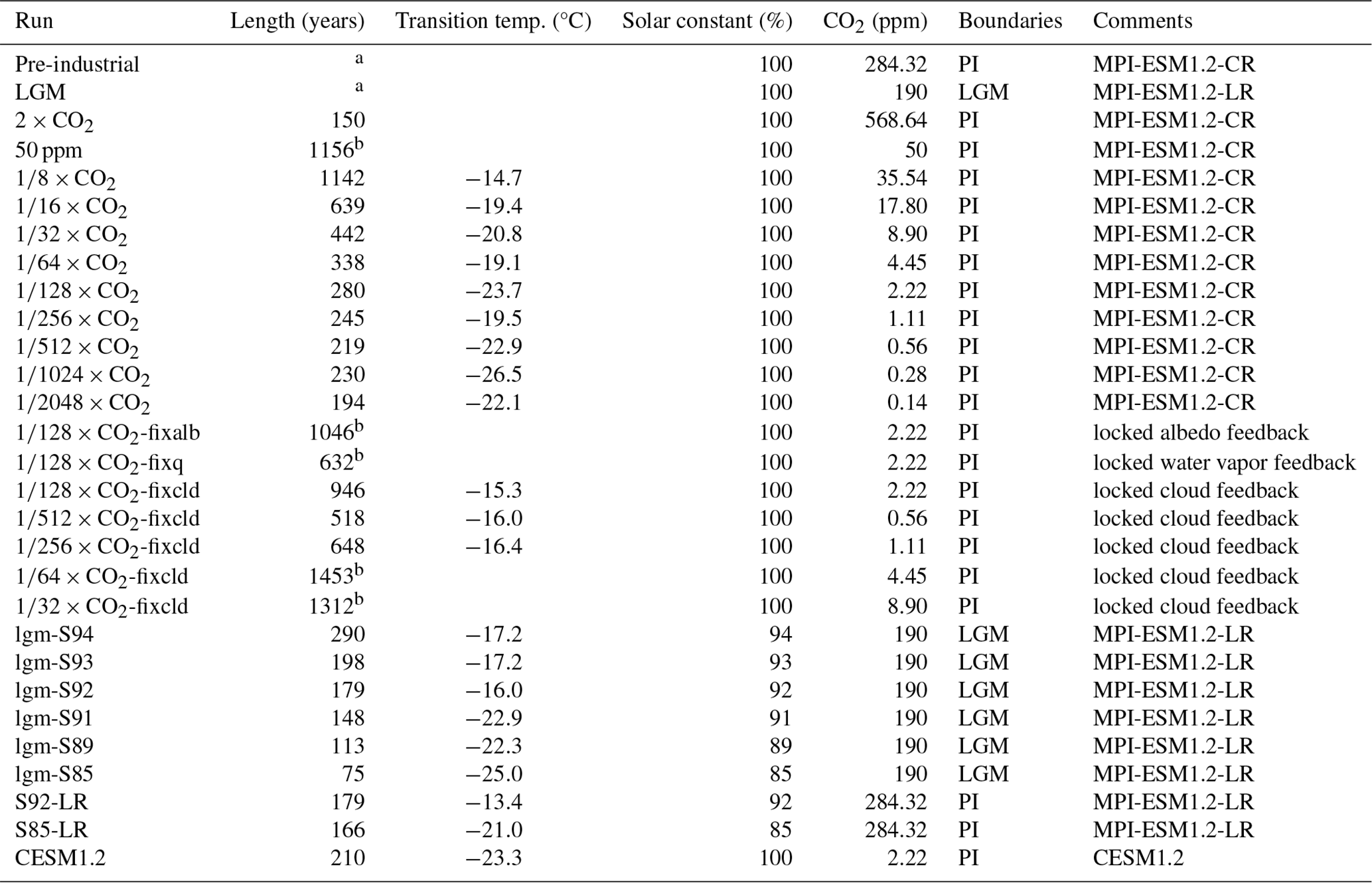
^a The runs started from an equilibrium state and ran for 100 years. ^b The runs were manually stopped and are expected to reach equilibrium in a cold non-snowball state. If the transition temperature is left empty, the simulation did not transit towards a snowball Earth during the years simulated.

The growth of thick sea ice leads to numerical instabilities in the ocean model component when exceeding 12 m. We do not artificially limit sea-ice growth, as was done in other studies (Voigt and Marotzke, 2010; Voigt et al., 2011; Voigt and Abbot, 2012), because this method generates latent heat at the base of sea ice (Marotzke and Botzet, 2007) which changes the required CO₂ forcing for snowball Earth initiation (Hörner et al., 2022). This results in all our simulations reaching numerical instability at some point when approaching a complete snowball Earth state due to the sea ice being too thick in narrow basins, such as the Baltic Sea. This does not affect our results, however, as we evaluate the transition in temperatures much higher than at the numerical instability. Only the 50 ppm simulation was manually stopped as it is expected to reach an equilibrium in a cold non-snowball state (see Table 1 for details on run length).

2.1 Temperature and imbalance evolution of the simulations

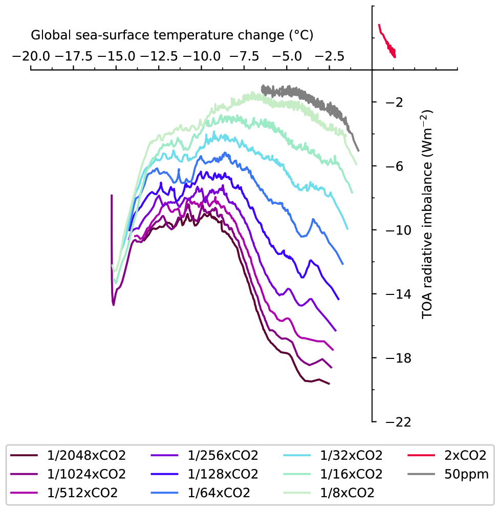
We analyse the evolution of our simulations by studying how the top-of-atmosphere (TOA) energetic imbalance changes with surface temperature. This approach is shown in Figs. 4 and 6 and has been first developed by Gregory et al. (2004). Here, each point of data is a one-year global average of the simulation as it responds to an initial and abruptly applied forcing. Because the total feedback is negative near the stable and stationary pre-industrial state, the system will attempt to reduce the TOA imbalance when exposed to positive or negative forcing. Consequently, in the case of an initial negative forcing from reduced CO₂ levels, the climate cools down. Therefore, the beginning of the simulation is where the temperature difference to PI is the closest to zero, and the imbalance is close to the forcing imposed. The end of the simulation is the left-most point, when the temperature anomaly relative to PI conditions is the largest.

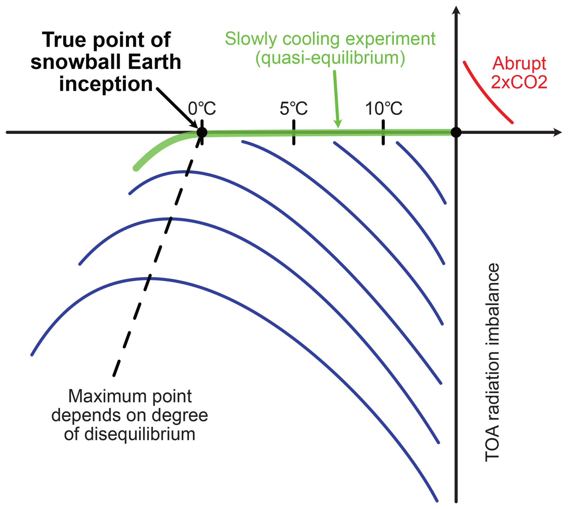
Figure 1 Schematic of top-of-atmosphere (TOA) imbalance vs. surface temperature difference to pre-industrial (PI), as developed by Gregory et al. (2004). Here, we compare the behavior of our abrupt forcing simulations, as they cool down, to the behavior of a real world transition wherein CO₂ is slowly and gradually reduced (green line). Note that the dashed line is added for illustration purpose only.

In the real climate system, the climate would slowly cool down as the forcing from the Sun or greenhouse gases change only slowly over time. Such transitions and abruptly forced simulations are illustrated in Fig. 1. When a negative forcing is slowly applied, for instance if CO₂ is slowly decreasing over time, the climate system would maintain a quasi-equilibrium and move along the green line to colder temperatures, until the true instability leading to a snowball Earth state is reached. In our simulations, the point closest to equilibrium, i.e. the least negative TOA imbalance, serves as to estimate the transition value. If a simulation was to be brought to higher CO₂ concentration, it is at this point that the equilibrium would be reached first. Because the simulations miss this equilibrium point, and since any other year is further out of balance than the year at this equilibrium point, they will not reach any other equilibrium until a new climate state, most likely the snowball Earth state, is found. Therefore, we can estimate the model's transition temperature towards snowball Earth as the temperature of the year with the least negative TOA imbalance. By definition it is also the year where the total climate feedback would be strictly zero before turning positive, which is represented by the tangential line in the Gregory et al. (2004) framework.

As we shall see, the simulated point slightly differs from the true transition point due to time-dependent effects that are proportional to the degree of disequilibrium. It appears that when the forcing is strongly negative, the transition point in the Gregory analysis shifts to lower temperatures. We speculate that this is a kind of time-dependent feedback effect whereby the positive feedback from formation of sea ice is delayed by the large thermal inertia of the oceans. Therefore, to estimate a model's true snowball Earth transition point it is necessary to carry out multiple abrupt forcing experiments as is done in this study.

2.2 Climate feedback calculations

Climate feedbacks are diagnosed using the partial radiative perturbation (PRP) method (Wetherald and Manabe, 1988; Colman and McAvaney, 1997). Details of its online implementation in MPI-ESM1.2 are in Meraner et al. (2013). The PRP method calculates individual contributions of surface albedo, clouds, temperature and water vapor changes to top-of-atmosphere fluxes, by exchanging related variables between a control climate state and the transient state analysed. Because the length of each run varies with the forcing amplitude, we compute climate feedbacks by regressing the top-of-atmosphere radiation balance changes arising from albedo, clouds, temperature, water vapor changes over bins of data points spanning a global temperature ranges of 5 °C. We apply the same method in the maps of Fig. 3, whereby the temperature indicated is the middle point of the temperature range.

We furthermore perform runs where we separately lock surface albedo, clouds or water vapor in the radiation calculations to the control state, i.e. the corresponding feedbacks do not contribute to the radiation balance. The implementation in MPI-ESM1.2 is described in Mauritsen et al. (2013). These locked-feedback transient simulations read the PI control albedo, clouds, temperature and humidity and impose them on the radiation parameterization regardless of the changes the system is experiencing, such as the increasing extent of sea ice.

2.3 Constraint on Earth's climate sensitivity

The relationship between LGM simulated temperatures and the climate sensitivity of models have been used in an emergent constraint framework to infer the Earth's true climate sensitivity owing to geological reconstructions of LGM temperatures (Hargreaves et al., 2012; Schmidt et al., 2014; Renoult et al., 2020, 2023). The novel constraint on Earth's climate sensitivity developed here uses the same relationship, derived from models participating in the Paleoclimate Modelling Intercomparison Project Phase 4 (PMIP4), where the regression parameters are calculated via ordinary least squares method. This constraint relies on the simple fact that the real LGM was a stable glacial climate and did not transition to a snowball state. Therefore, Earth's climate sensitivity could not have been higher than the point at which the planet would transition into a snowball state before the LGM. As such, the presented constraint provides a physical upper bound on ECS, not a best estimate.

Recently, Renoult et al. (2023) showed that structural uncertainties and temperature-dependencies in climate feedbacks hinder the relationship between LGM temperature and climate sensitivity, which is computed from warm simulations (4 times pre-industrial CO₂ Gregory et al., 2004). The authors minimized the issue by adding to the PMIP4 ensemble an ensemble of CESM models (“CESM-family”, i.e. CESM1.2, CESM1.3 and low-ECS versions of CESM2), as the relationship also benefits from PMIP4 models to have a wider range of climate sensitivity, and because without these models, the relationship can be considered as too dependent on CESM2 (Renoult et al., 2023). We have added a similar test as conducted by Renoult et al. (2023) on tropical temperatures in Appendix B, where we show that on a global scale, CESM2 and the CESM-family ensemble are almost exchangeable, leading to a robust relationship with similar slopes and intercepts in both cases. Therefore, as we only have access to the sea-surface temperature data of the CESM-family ensemble, whereas our analyses are mostly based on surface temperatures including land, we use CESM2 for most of our study. This is on the basis that as the CESM-family ensemble is not an outlier, and it is exchangeable with CESM2, therefore the consequences of CESM2 being in the PMIP4 ensemble are also not due to it being an outlier. Since models from the same institutes can sometimes introduce larger differences than between models from different modelling centers (Knutti et al., 2013), we would like to emphasize that it is not an ideal solution with the low number of paleosimulations available, and sometimes limited data, but should be seen as motivation for institutes with higher climate sensitivity models to perform and publish LGM runs regardless of whether they are stable or transition towards a snowball state.

3 Analysis of surface albedo and cloud feedbacks

We perform experiments with abrupt decreases of CO₂ concentrations ranging from $\mathrm{1}/\mathrm{8}$ to $\mathrm{1}/\mathrm{2048}$ of PI CO₂ concentration using the MPI-ESM1.2-CR model to simulate snowball Earth transition and break down climate feedbacks (Sect. 2). The strengthening surface albedo feedback has often been considered the main driver in the snowball Earth instability, yet positive cloud feedbacks exceed the surface albedo feedback during the initial 10 °C of cooling, relative to PI (Fig. 2). This strengthening arises from positive tropical cloud feedbacks (Fig. 3) due to an increase in shallow cloud coverage over the tropical oceans (Appendix Fig. C1). Cloud feedbacks are increasingly more positive as the initial forcing is increasingly stronger, which amplify tropical cooling. Below −20 °C relative to PI, cloud feedbacks switch sign and are globally negative and weaker than the surface albedo feedback, although there still exists strong positive cloud feedbacks ahead of the advancing sea-ice edge in both hemispheres (Fig. 3). Indeed, because the sea-ice surface is cold, clouds are preferentially over open water which is warmer and a source of moisture (e.g. Wall et al., 2017), where they facilitate further cooling of the ocean. All in all, cloud feedbacks substantially contribute to early cooling in response to reduced CO₂. During the transition, the positive surface albedo feedback starts to exceeds the combined cloud, temperature and water vapor feedbacks at temperatures between −15 and −20 °C below PI (Fig. 4). This leads to a global instability and is concomitant with the acceleration of the equatorward sea-ice edge into the sub-tropics, resulting in strong global cooling towards the snowball state.

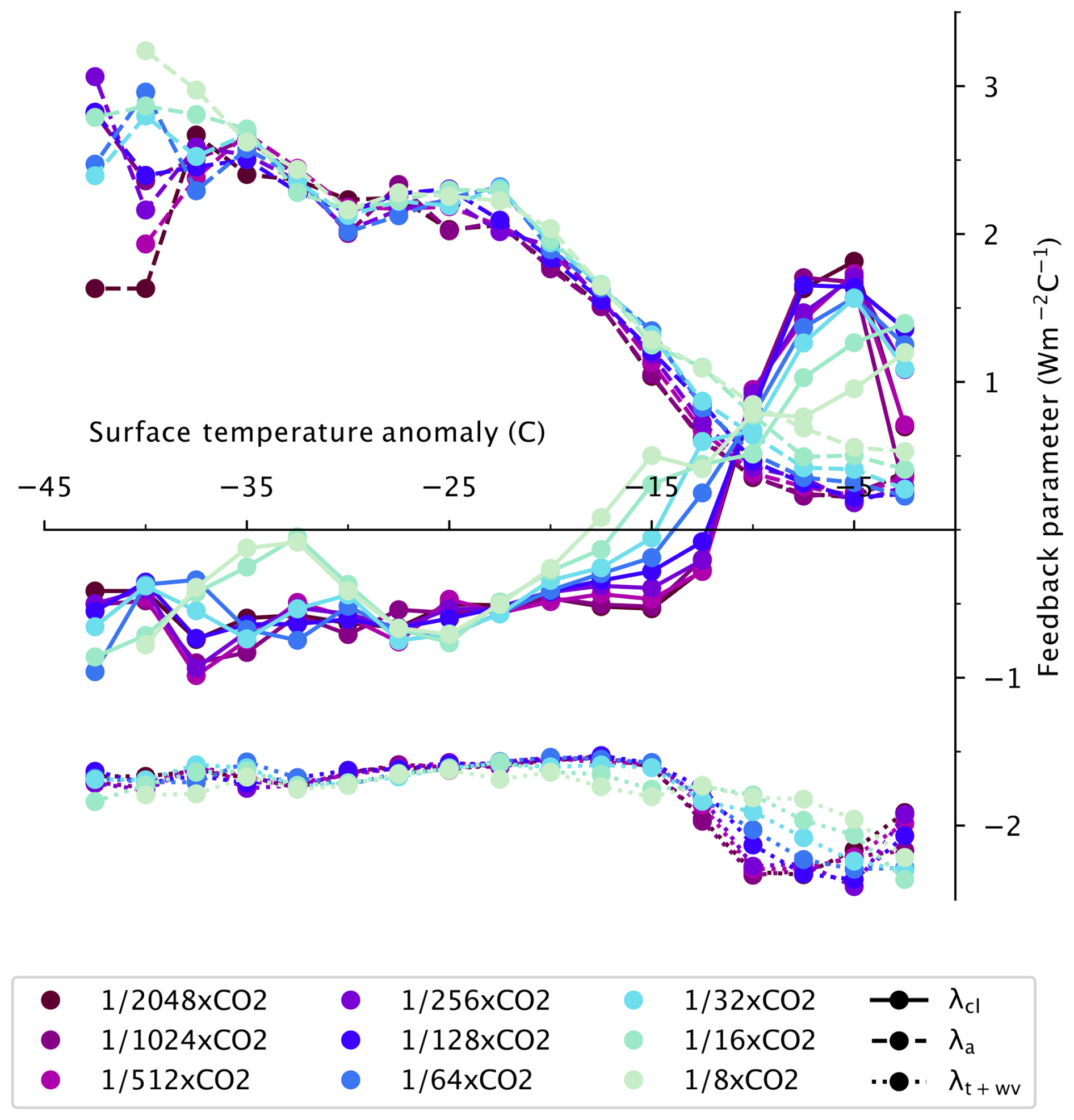
Figure 2 Evolution of the climate feedback parameters of clouds (λ_cl), albedo (λ_a) and temperature and water vapor combined (λ_t+wv) with global surface temperature anomaly compared to pre-industrial (PI) (°C) under all CO₂ forcing.

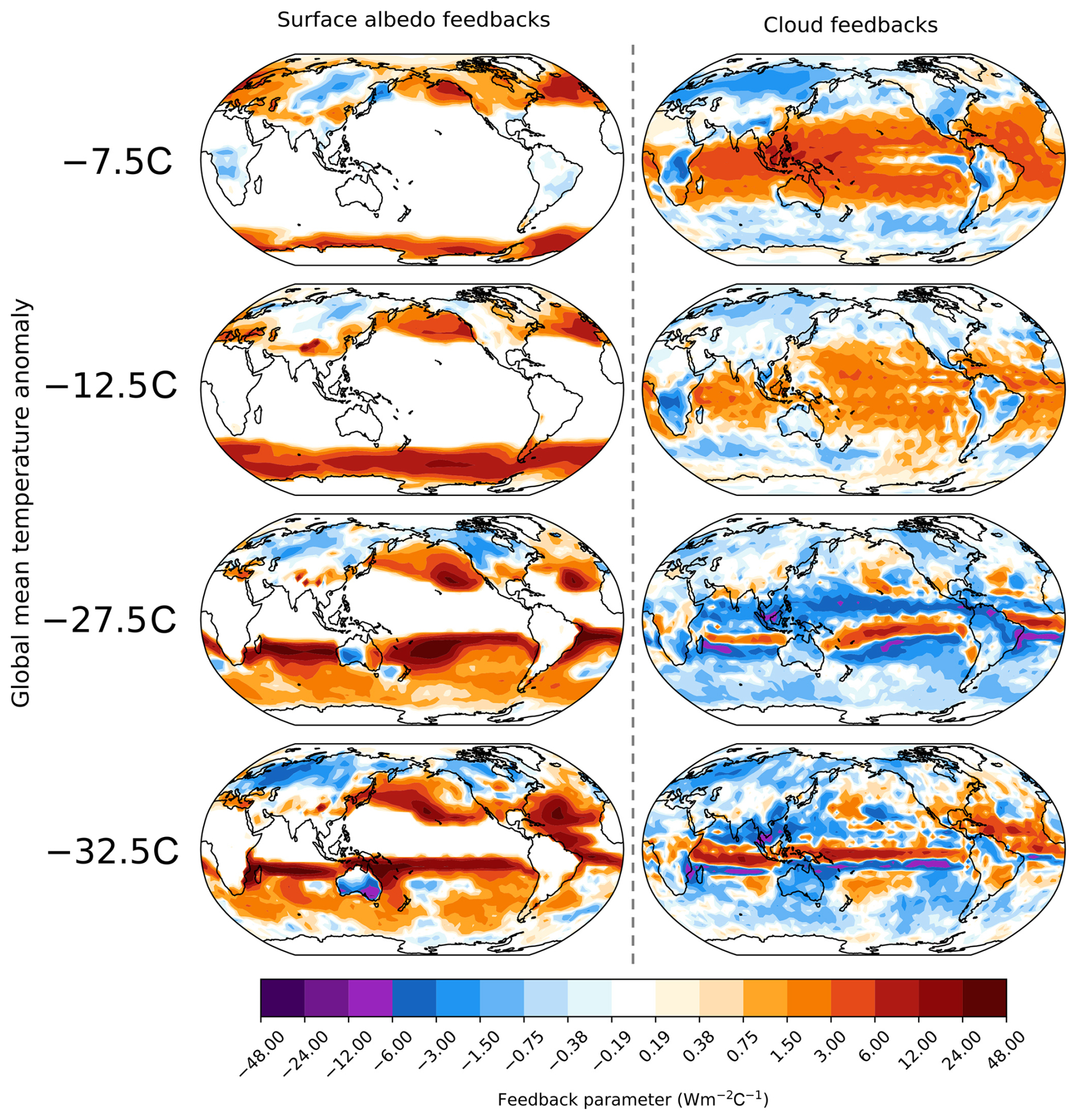
Figure 3 Maps of the surface albedo (left column) and cloud (right column) feedbacks at four average global temperatures in the $\mathrm{1}/\mathrm{16}\times {\mathrm{CO}}_{\mathrm{2}}$ simulation. The global mean temperature anomaly indicated is the middle point of the temperature range over which the feedbacks are computed, taking bins of 5° of cooling.

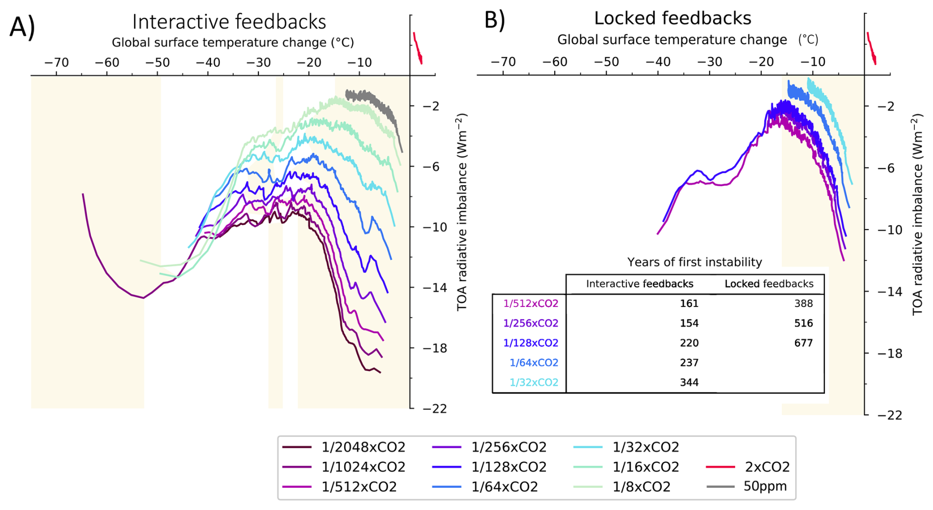
Figure 4 (A) Top-of-atmosphere (TOA) radiative imbalance (Wm⁻²) vs. global surface temperature anomaly relative to pre-industrial (PI) conditions (°C) under varying CO₂ forcing and (B) same but with cloud feedbacks locked to that of the control state. A run with an abrupt doubling of CO₂ (2×CO₂) is shown for comparison. The 50 ppm run was manually stopped due to its large computational cost. Colored phases correspond to negative feedback, white phases positive feedback. The years of the first instability between interactive and locked feedbacks are annotated.

The diagnostics presented above are suggestive that cloud feedback may be an important climate driver towards the snowball transition. To demonstrate that this is indeed the case, we isolate the importance of each feedback using the feedback locking technique (Sect. 2) on various simulations, where each feedback mechanism is disabled one after the other (Fig. 4B). When the cloud feedback is locked, the instability is reached at a similar global mean temperature as in the non-locked simulations, between −15 and −20 °C relative to PI (Fig. 4A). However, cloud feedback locking drastically increases the forcing required to initiate the snowball Earth transition, and considerably slow down the transition to snowball Earth. We find that simulations at CO₂ concentration of $\mathrm{1}/\mathrm{64}$ times PI levels and lower are required to trigger the transition with locked cloud feedbacks, which is a factor ten less than the concentration required with interactive cloud feedbacks. The surface albedo-locked simulation does not reach a snowball instability as it enters quasi-equilibrium below the transition temperature of around −15 °C relative to PI. Similarly, the simulation reaches a quasi-equilibrium below −10 °C relative to PI when the water vapor feedback is locked (Appendix Fig. C2). The water vapor feedback actually does not strengthen with cooling so is not itself the cause of the snowball instability, however its large positive feedback is important for allowing the surface albedo to trigger the instability. Thus, the role of cloud feedback is different from that of the surface albedo feedback: (1) positive cloud feedbacks facilitate an early tropical cooling, and this effect is increased with stronger negative forcing, (2) positive cloud feedbacks ahead of the advancing sea-ice edge and its effect on tropical oceans accelerate the transition to snowball Earth and decrease the temperature of instability, as summarized in Fig. 5; (3) cloud feedbacks substantially increase the threshold CO₂ level required for snowball Earth initiation and (4) the advance of sea ice into the southern subtropics results in the surface albedo feedback exceeding the sum of the negative feedbacks. Whereas the surface albedo feedback is responsible for the transition and the main driver to the complete glaciation, our results emphasise an important contribution of cloud feedbacks. Cloud feedbacks are also the main cause of inter model spread in climate sensitivity (e.g. Zelinka et al., 2020), a fact which we shall exploit in Sect. 5.

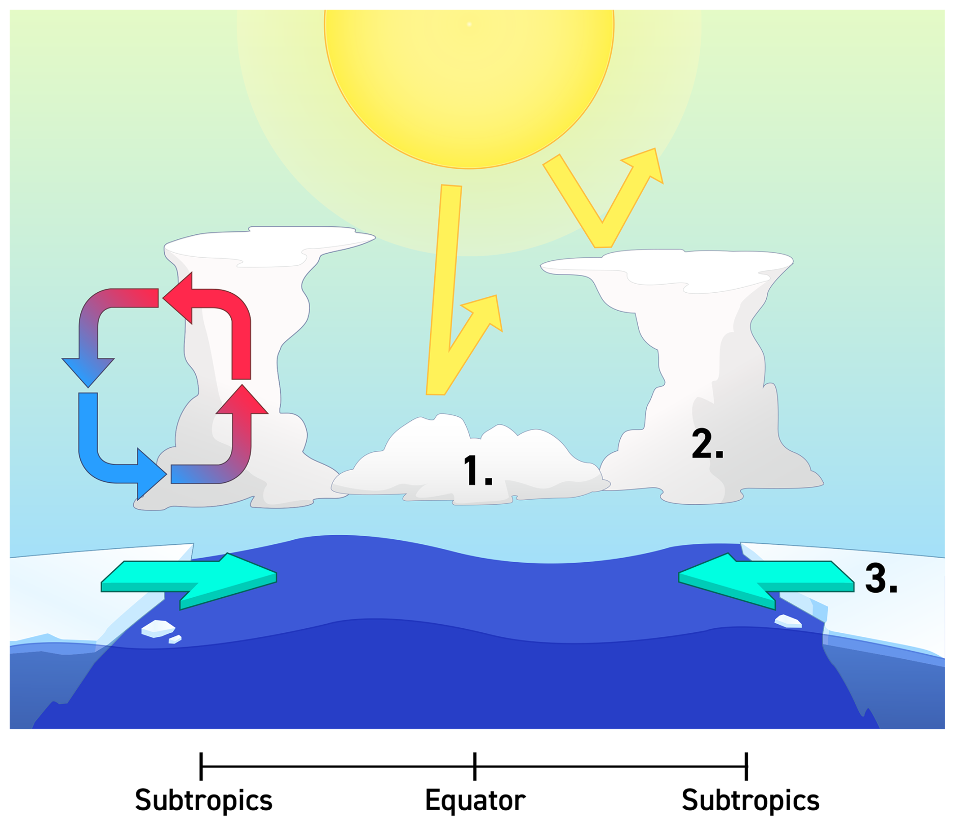
Figure 5 Contribution of cloud feedbacks to ocean cooling and interaction with sea ice. (1) Tropical surface cooling by positive low-level cloud feedback. (2) Sea surface cooling ahead of ice edge. (3) Faster sea-ice advance, facilitated by winds pushing sea ice equatorwards (Appendix Fig. C3).

4 Model evidence for the snowball transition temperature

The temperature at which the climate transits towards a snowball Earth state is broadly similar across the different CO₂ forcing experiments (Fig. 4), when taking into account that it depends systematically on the degree of disequilibrium (Fig. 1). This is independent of whether the experiment is initialized from a PI or an LGM state, as shown in Appendix A, which demonstrates the importance of background temperature control over the climate feedbacks which drive the transition. In particular, sea-ice formation is primarily temperature-dependent, and the amplitude of the sea-ice albedo feedback is practically independent of the strength of the negative forcing (Fig. 2). We can expect such temperature-dependency to be similar across climate models, which would contribute to them having a similar temperature of entering the snowball transition. Similarly, the winds push sea ice equatorwards (Appendix Fig. C3), in connection with temperature contrast between sea ice and open ocean. This is concomitant with positive cloud feedbacks ahead of sea-ice edge, which is expected to behave in similarly across models since they broadly represent the same general circulation. A simple geometric argument for a transition temperature close to 0 °C is that it happens when the ice edge enters the sub-tropics at about 30° latitude, leaving about half the Earth still ice free and hence above the freezing temperature, and the other half at temperatures below. When abruptly decreasing the CO₂ concentration to 50 ppm (around $\mathrm{1}/\mathrm{6}$ of PI CO₂), we find hints of instability near the global mean temperature of 0 °C (near −15 °C relative to PI), but the model is stable for 1848 years until it crashes due to thick sea ice (Sect. 2). This indicates that it is unlikely that the transition temperature happens at a temperature substantially warmer than 0 °C.

Nevertheless, the transition temperatures of each phase show a slight shift to lower values under stronger negative forcing. Therefore, the climate system deviates from pure temperature-dependent behaviour as the strength of the radiative cooling and the speed of transition to snowball Earth increases. These time-dependent effects have often been described in the literature following extreme cooling rates (Bendtsen and Bjerrum, 2002; Marotzke and Botzet, 2007), and we speculate that this is due to the large heat capacity of the ocean, as well as differences in ocean mixed layer depths and direct CO₂ forcing across different regions: in certain circumstances, this can result in local temperatures dropping faster than global temperatures (Appendix Fig. C4A), and hence out of sync with the sea-ice extent controlling the surface albedo feedback. Ocean convective mixing is also increasingly more efficient at evacuating heat for larger surface cooling, indicated by an increasing peak of the strength of the Atlantic meridional overturning circulation (AMOC) in Appendix Fig. C4B. The associated ocean currents on the contrary drag sea ice polewards and can slow down the sea-ice edge advance (Voigt and Abbot, 2012). All in all, we suggest slow, low forcing simulations are preferable when analysing snowball Earth transitions, as (1) fast transitions to snowball Earth are hardly realistic, as geological snowball states may form over millions of years (e.g. Schrag et al., 2002) and (2) fast transitions involve temporal effects which would depart from temperature-dependency. All together, these considerations support the transition temperature close to 0 °C found in the experiments with weak forcing.

5 Potential constraint on climate sensitivity

While we expect the temperature-dependency to behave similarly across models, it is currently not known whether the temperature threshold of 0 °C that we find in MPI-ESM1.2-CR is indeed universal. The CESM model family has performed several snowball Earth simulations (Yang et al., 2012a, b; Eisenman and Armour, 2024), and while the model CESM2 also transits towards a snowball Earth around 0 °C under similar CO₂ forcing (Eisenman and Armour, 2024), models such as CCSM3 and CCSM4 can have stable waterbelt states with abrupt but smaller transitions, which anyway are not likely consistent with the evidence for recent LGM states. To further test this, we perform an abrupt $\mathrm{1}/\mathrm{128}\times {\mathrm{CO}}_{\mathrm{2}}$ simulation with the model CESM1.2. At $\mathrm{1}/\mathrm{128}\times {\mathrm{CO}}_{\mathrm{2}}$, CESM1.2 shows a transition temperature at around −24 °C below pre-industrial, or approximately −10 °C absolute temperature, which is similar as MPI-ESM1.2 at the same forcing level (Fig. 6). Due to the time-dependent effects, which we discuss in this study, the transition temperature is displaced under strong forcing. Therefore, under a low forcing, we expect the transition temperature to be closer to 0 °C for CESM1.2, as was the case for MPI-ESM1.2.

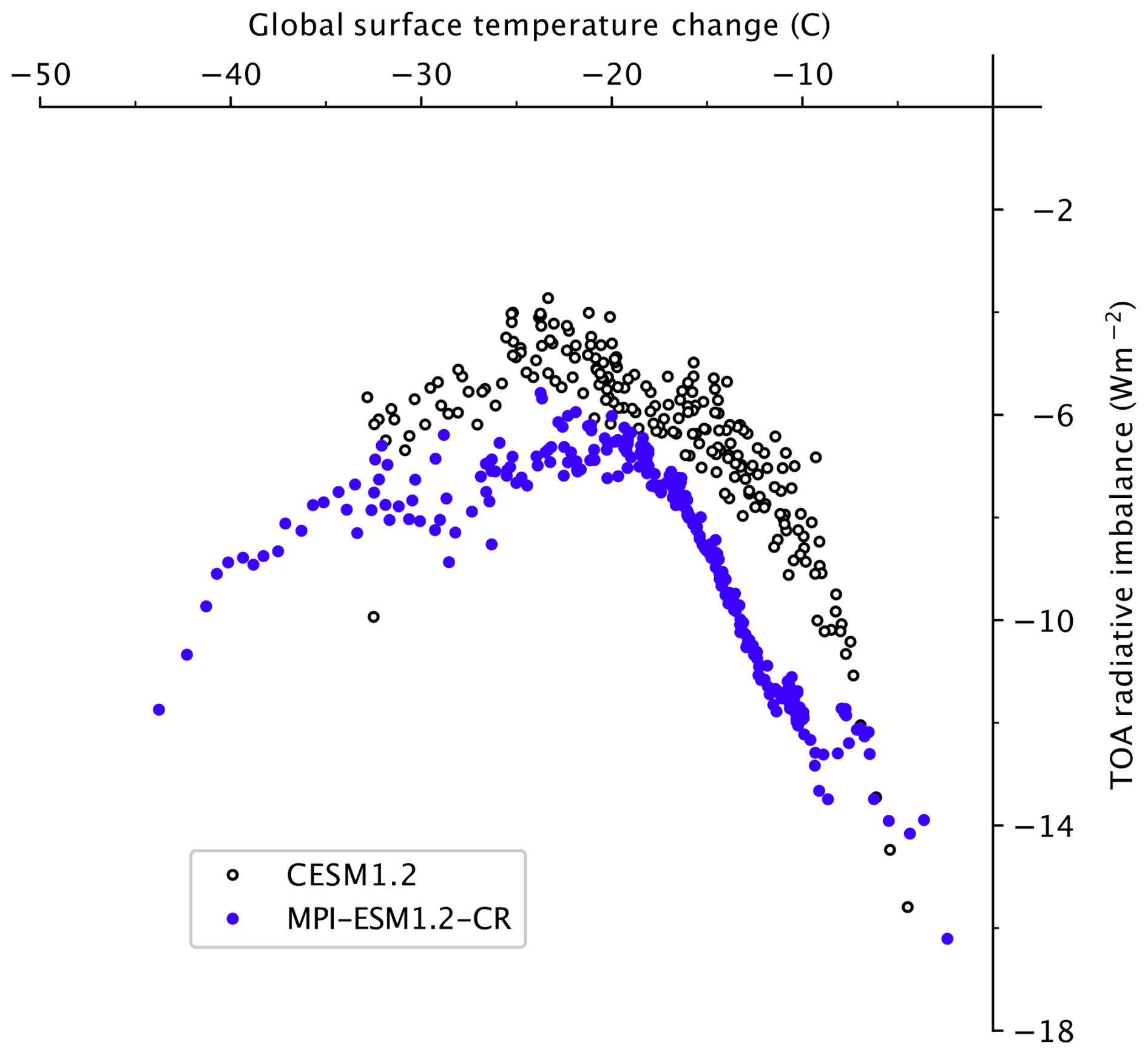
Figure 6 Top-of-atmosphere (TOA) radiative imbalance (Wm⁻²) vs. global surface temperature anomaly relative to pre-industrial (PI) conditions (°C) in abrupt $\mathrm{1}/\mathrm{128}\times {\mathrm{CO}}_{\mathrm{2}}$ simulations with the models MPI-ESM1.2-CR and CESM1.2.

There is an ongoing discussion on whether climate models with large cloud feedbacks and consequently high climate sensitivity are compatible with the LGM (Zhu et al., 2022; Burls and Sagoo, 2022). Models with high climate sensitivity simulate LGM temperatures around the snowball Earth transition temperature of around 0 °C and are usually unstable. This in fact is to be expected if the transition temperature is controlled by the temperature-dependent behaviour of the climate feedbacks, where the threshold before transiting to a snowball Earth state would be similar across models. In the case of tropical shallow cloud feedbacks, despite considerably increasing the sensitivity of the climate to enter snowball Earth, they do not seem to affect the snowball Earth transition temperature itself (Fig. 4).

It is therefore possible to estimate an upper limit of climate sensitivity from the models with stable LGM states with an emergent constraint framework (Sect. 2), using as snowball temperature threshold a global mean temperature close to 0 °C. In this way, we find that it is implausible that climate sensitivity exceeds 6.2 °C (3.9 %–8.4 %, 5 %–95 % confidence interval, Fig. 7). This upper limit is close to the sensitivity of CESM2 (5.6 °C), which simulates an LGM temperature anomaly of −11.3 °C (Zhu et al., 2021), just above the global mean temperature of 0 °C. Additional support for this upper limit is obtained from a slightly more sensitive version of the model, which is unstable when run under LGM boundary conditions (Zhu et al., 2022).

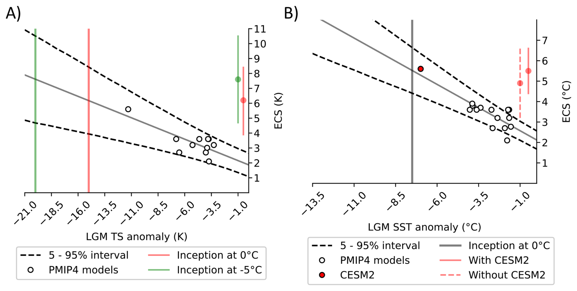
Figure 7 Relationship between modelled LGM surface temperature anomaly relative to pre-industrial (PI) and the climate sensitivity of PMIP4 models. The upper bound on climate sensitivity can be constrained using the temperature at which the climate starts transiting to snowball Earth, which is different whether it is from surface temperatures or sea-surface temperatures. In (A), the threshold is around −15 °C global mean surface temperature anomaly relative to PI (red), and in (B), the corresponding threshold as seen in sea-surface temperatures is around −7.5 °C relative to PI (grey). Several sensitivity tests for the computation of the upper bound on climate sensitivity are shown: (A) if the upper bound of the transition was instead at −20 °C relative to PI (green), and (B) if CESM2 is left out of the ensemble, but the other CESM models are included, where only sea-surface temperatures are available.

On account of the uncertainty on whether the transition temperature would be close to 0 °C across models, we test the sensitivity of our constraint by decreasing the transition temperature to −5 °C (Fig. 7). In this case, we find that the upper bound on ECS cannot exceed 7.6 °C (4.7 %–10.5 %, 5 %–95 % confidence interval). This is a relatively modest change of 1.4 °C in the upper bound, considering the large change in transition temperature of −5 °C. The uncertainty on the transition therefore has a small influence on our upper bound ECS estimate, and the value obtained here is in agreement with estimates from other lines of evidence, or is in many cases a stronger constraint (Forster et al., 2021).

Finally, we further test the sensitivity of the upper bound estimates on climate sensitivity using the sea-surface temperature threshold (estimated at close to −7.5 °C using the same approach as in Fig. 1, in Appendix C5), which allows us to include the CESM-family ensemble described in Sect. 2, and leave CESM2 out of the ensemble. When the CESM-family ensemble is included, and whether CESM2 is or is not in the ensemble, the relationship is robust and displays similar characteristics (Appendix B). The inclusion of CESM2 strengthens the relationship and increases the constraint on the upper bound on climate sensitivity, but also increases the median estimates to 5.5 °C (4.4 %–6.6 %, 5 %–95 % confidence interval), in comparison to 4.9 °C (3.2 %–6.7 %, 5 %–95 % confidence interval) when CESM2 is excluded. As such, the results are not overly sensitive to the inclusion of CESM2, but overall confidence in the constraint would be significantly strengthened if more institutes would perform the LGM simulations.

6 Motivation for simulations

The described approach to provide an upper bound on climate sensitivity could have a great potential, in particular as independent constraints from paleoclimates are found to be increasingly useful (Sherwood et al., 2020; Forster et al., 2021). Nevertheless, to support the constraint, it would be beneficial that modelling centres publish their LGM simulations, even if they fail to stabilise, as this may be used to narrow down the uncertainty on the instability threshold.

It is also important to know whether many models have a threshold gravitating around 0 °C, similarly to that found for MPI-ESM1.2-CR, MPI-ESM1.2-LR and CESM1.2. To tackle this latter problem, we suggest the following experimental design, which is short and easy to replicate:

1. Run a PI state, with the CO₂ concentration set to $\mathrm{1}/\mathrm{128}$ times the PI value, until the model reaches at least the initial instability leading to the snowball Earth state. The chosen CO₂ concentration should be a fair trade off between a relatively short simulation length and the time-dependency effects discussed in this study. If time allows, complement with less strong reductions to investigate the time-dependency.

2. Generate a plot of top-of-atmosphere radiation imbalance vs. surface temperature anomaly relative to PI, as in Fig. 4. Report the instability threshold temperature, from surface and sea-surface temperature, as well as the global sea-ice distribution.

The results could support the novel constraint on climate sensitivity presented in this study, but also help understanding the challenges that some modeling groups experience in LGM simulations, a paleoclimate notoriously difficult to model. We advocate that multi-model comparisons of snowball Earth transitions, as well as single-model ensembles with varying climate sensitivity, would better support the relationship between simulated LGM temperatures and the upper bound on climate sensitivity. The main strength of this constraint is that it is independent of paleoclimate reconstructions and simply relies on the fact that Earth did not undergo a transition to a snowball state 21 000 years ago, or during any earlier glacial cycles during the Pleistocene, providing a valuable additional line of evidence to those already used in the community (Sherwood et al., 2020; Forster et al., 2021).

Appendix A: Snowball state under solar forcing and from LGM conditions

We verify how snowball Earth transitions differ when starting from LGM or PI conditions. MPI-ESM1.2-LR is numerically unstable at low CO₂ concentrations, so we compare solar-forced snowball Earth transitions between LGM and PI instead.

The LGM is characterized by large ice sheets and lower sea-level which can affect cloud feedbacks as well as global circulations (Muglia and Schmittner, 2015; Sherriff-Tadano et al., 2018; Zhu and Poulsen, 2021a; Renoult et al., 2023), thus can influence the transition to a snowball Earth state. Changes in continental distribution and ocean areas are known to affect transition temperatures. For instance, Voigt et al. (2011) indicates a snowball Earth transition at 96 % of PI solar constant and PI CO₂ concentration with Marinoan reconstructed paleogeography (∼635 million years ago), which is characterized by agglomerated, bare-soil tropical continents, whereas it would require 94 % or lower with PI continents. Tropical land masses reflect more radiations and therefore contribute substantially to snowball Earth transitions.

When initializing from LGM conditions (Fig. A1), the same main phases of negative and positive feedbacks are identified than from PI conditions. There are slight differences between both cases, for instance the LGM simulation show a single instability phase, whereas the runs starting from PI still display hints of multiple phases when the solar constant is set at 85 % of PI value. However, the transition temperature connected to the main instability leading to the snowball Earth state happens at a broadly similar temperature than from PI conditions, between −15 and −20 °C relative to PI, which demonstrate the role of the feedback dependency on temperature, irrelevant of the differences in boundary conditions.

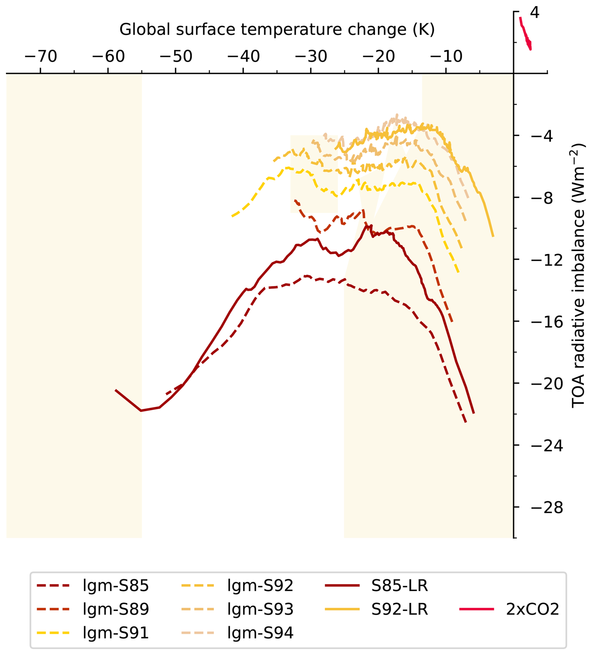
Figure A1 Top-of-atmosphere radiative imbalance (Wm⁻²) vs. global surface temperature anomaly relative to PI conditions (°C) under solar forcing from LGM conditions. Colored phases correspond to negative feedback, white phases positive feedback.

Memory effects are expected to differ from LGM and PI conditions and likely explain the slight differences in transition temperatures towards the snowball state. Indeed, the LGM ocean is colder than in PI, and the initial thermal state of the ocean is known to affect the speed at which the snowball state is reached (Bendtsen and Bjerrum, 2002). From the LGM, reaching snowball Earth is therefore easier, as tropical oceans are colder and the evacuation of heat via ocean mixing is enhanced. This should add further in rendering the LGM simulations difficult for modern climate models, as they usually initialise their experiments from LGM states of previous generations.

Appendix B: Emergent constraint on climate sensitivity from LGM global temperatures

We analyse how sensitive the emergent constraint framework based on PMIP4, described in Methods and used in Fig. 7 is to the presence of CESM2, and whether the PMIP4 ensemble can be used in this study. Due to its high climate sensitivity, CESM2 is often seen as an outlier in the PMIP4 ensemble, which could bias statistical analysis. A solution used by Renoult et al. (2023) was to expand the PMIP4 ensemble with lower-ECS versions of CESM models, as to widen the ECS range of the PMIP4 ensemble and minimize the outlier effect of CESM2. Renoult et al. (2023) also showed that for the sake of the characteristics of the relationship (slope, intercept), as well as significance and predicted ECS, CESM2 and this lower-ECS CESM-family ensemble were in fact exchangeable if the relationship was based on tropical LGM sea-surface temperatures.

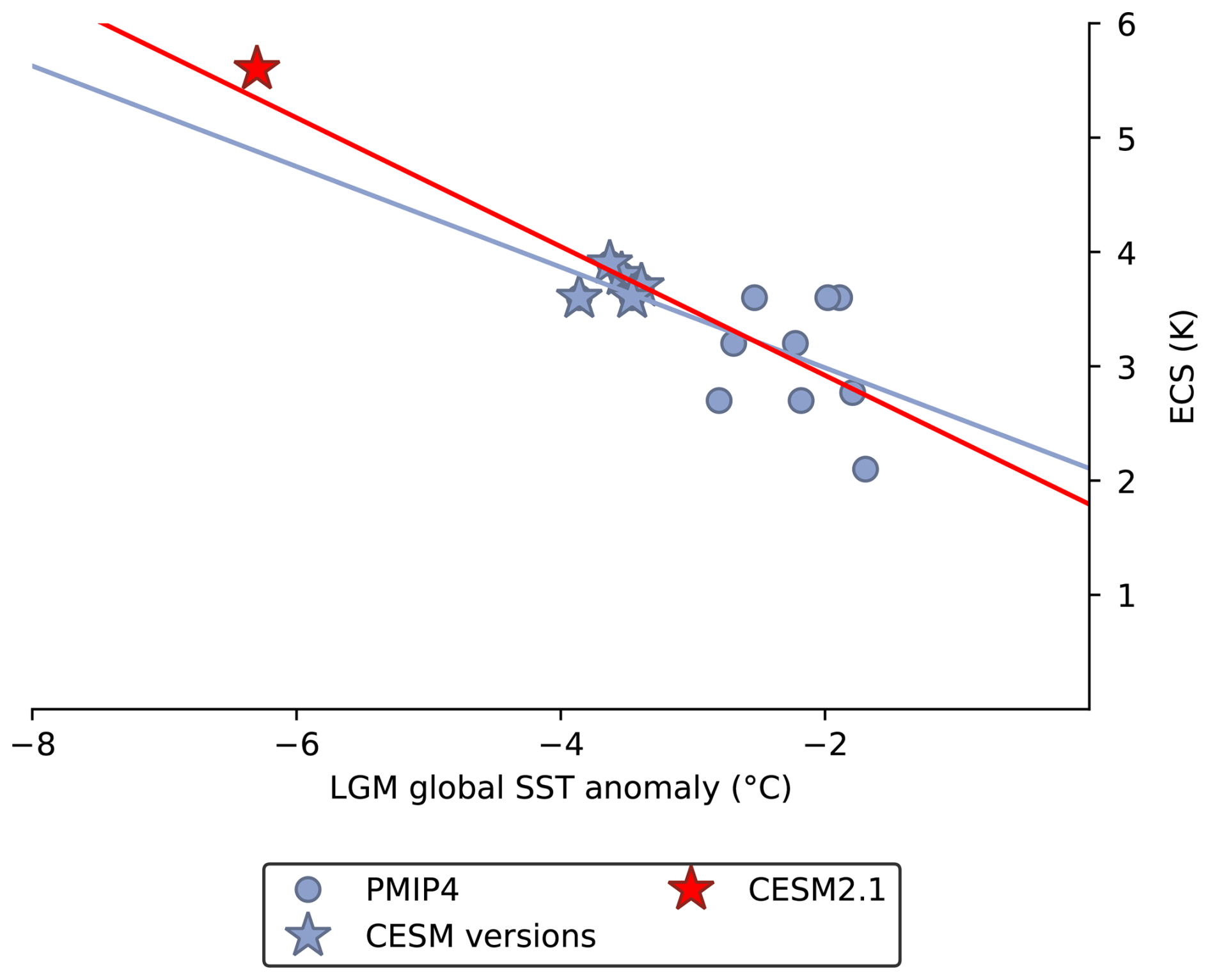
Figure B1 Emergent constraint relationship on climate sensitivity using LGM global sea-surface temperatures relative to PI state. Two relationships are compared: one using the original PMIP4 ensemble (PMIP4 models and CESM2; red relationship) and one using the extended ensemble (PMIP4, CESM2 and the CESM-family models; blue relationship).

During the LGM, emergent-constraint based relationships were often found to be more significant when based on tropical temperatures, either because it could minimize the uncertainties on extra-tropical forcing (Hargreaves et al., 2012; Renoult et al., 2023) or simply because variations on climate sensitivity were more sensitive to tropical climate feedbacks during PMIP2 (Hargreaves et al., 2012). However, there is no reason that the relationship would not exist when based on global temperatures, as one could still expect a correlation between global temperatures and climate sensitivity, which is essentially a CO₂-based metric.

In Fig. B1, we use the temperatures of Renoult et al. (2023) and references within, as to verify whether on a global scale CESM2 and the CESM-family ensemble are also exchangeable, and if consequently CESM2 only acts as an outlier. We find the same conclusions as Renoult et al. (2023) on tropical sea-surface temperatures: a relationship which includes the PMIP ensemble (without CESM2) and the CESM-family ensemble has similar slopes, intercept, and is as significant as a relationship with the PMIP4 ensemble and CESM2 (without the CESM-family ensemble), where in both cases the p values are below 0.05. Therefore, the PMIP4 ensemble is sensitive to a wider range of ECS rather than CESM2 itself (Renoult et al., 2023).

Appendix C: Additional figures

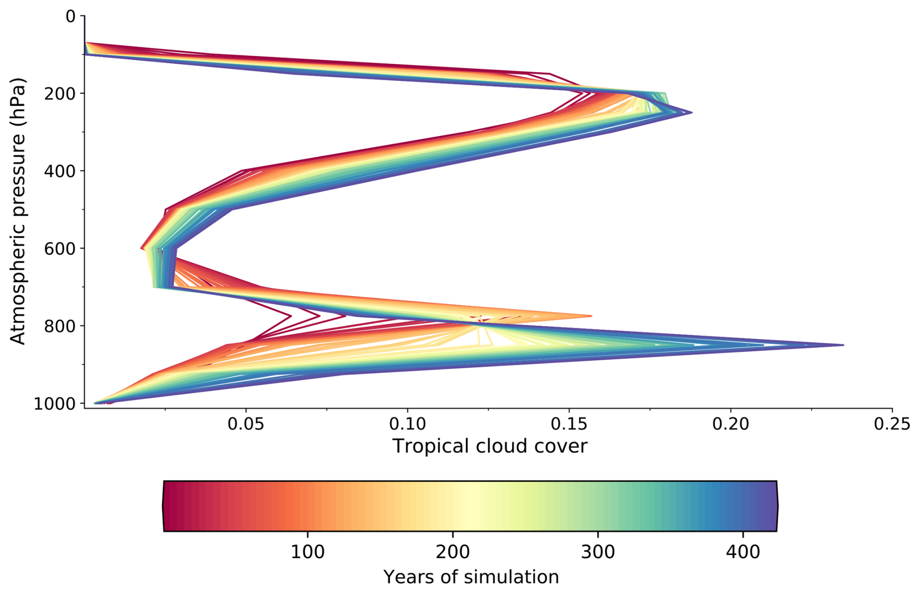
Figure C1 Evolution of tropical (30° S–30° N) cloud cover within the first 15 °C of cooling (425 years of simulation) in the $\mathrm{1}/\mathrm{16}\times {\mathrm{CO}}_{\mathrm{2}}$ simulation.

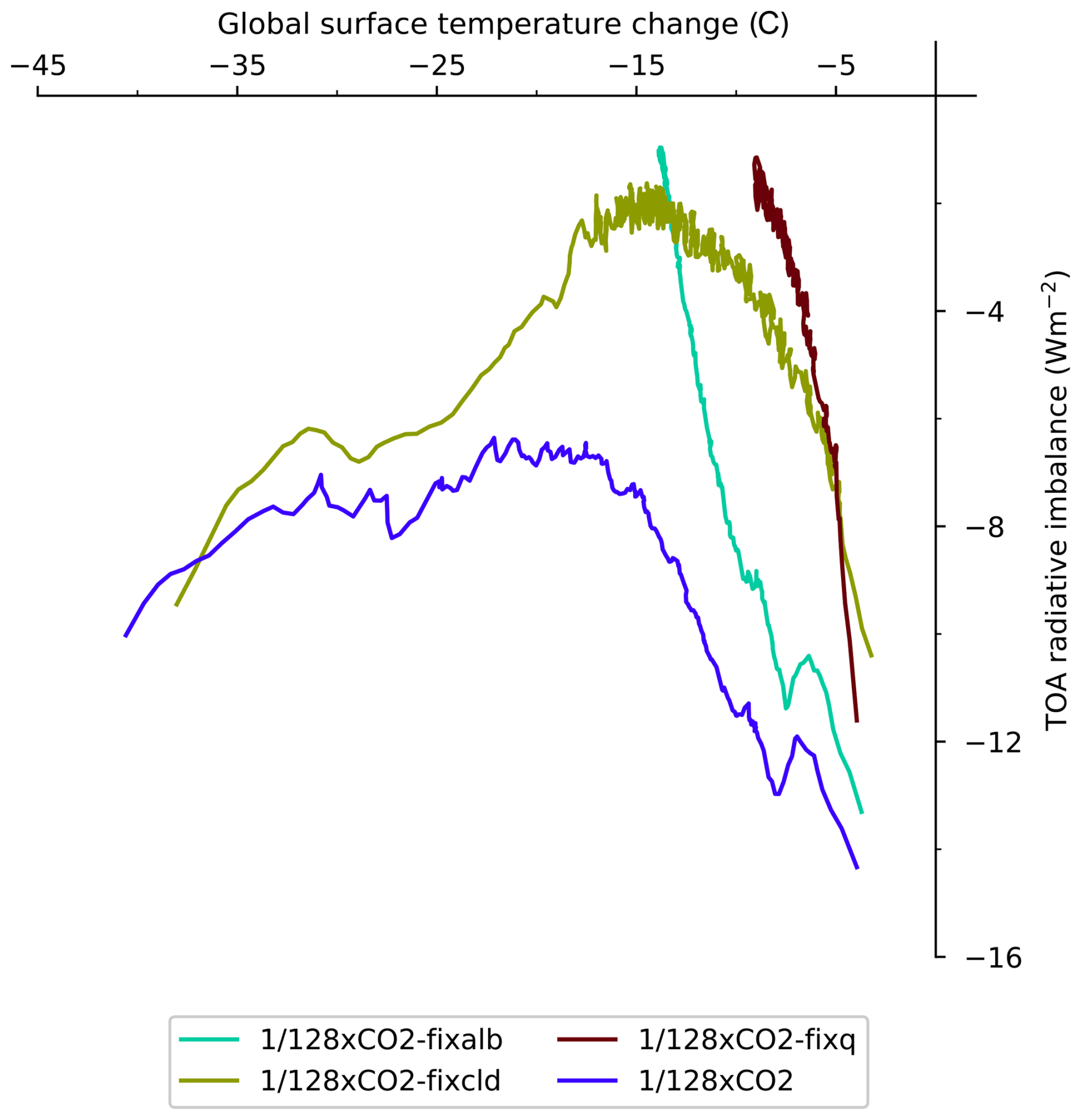
Figure C2 Top-of-atmosphere radiative imbalance vs. global surface temperature anomaly relative to PI conditions for the $\mathrm{1}/\mathrm{128}\times {\mathrm{CO}}_{\mathrm{2}}$ simulation with either surface albedo (fixalb), water vapor (fixq) or cloud (fixcld) feedbacks locked to that of the control state.

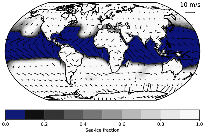
Figure C3 Surface wind field on sea-ice cover during the snowball Earth transition for the $\mathrm{1}/\mathrm{16}\times {\mathrm{CO}}_{\mathrm{2}}$ simulation. Strong winds push sea ice equatorwards in the tropical regions.

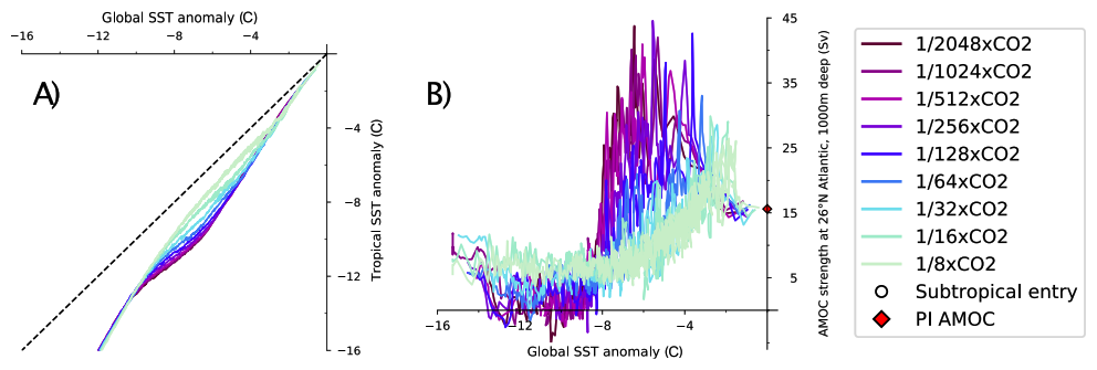
Figure C4 Analysis of tropical and global components affecting the rate of snowball Earth transitions. (A) Differences in tropical and global sea-surface temperature cooling under all CO₂ forcing. (B) Strength of the Atlantic meridional overturning circulation (AMOC) measured at 26° N, 1000 m deep (Sv) under all CO₂ forcing. The average PI AMOC strength, around 16 Sv, is highlighted.

Figure C5 Top-of-atmosphere radiative imbalance (Wm⁻²) vs. global sea-surface temperature anomaly relative to PI conditions (°C) under the same CO₂ forcing as Fig. 4. When using sea-surface temperatures, the transition happens at around −7.5 °C relative to PI for the lowest forcing ($\mathrm{1}/\mathrm{8}\times {\mathrm{CO}}_{\mathrm{2}}$).