Dynamical system metrics and weather regimes explain the seasonally-varying link between European heatwaves and the large-scale atmospheric circulation

Global warming is projected to increase the frequency and intensity of heatwaves in the extended summer period. To better predict heat extremes, it is important to explore the seasonal variations in their drivers. Therefore, we analyze heatwaves in Central Europe using ERA5 reanalysis data over the historical period (1950–2023) for the extended summer months (May–September). We quantify atmospheric persistence, and the link between near-surface temperatures and large-scale atmospheric circulation patterns using dynamical system metrics. This approach is further contextualized by the consideration of weather regimes, which represent the low-frequency variability of the atmosphere over the North Atlantic and Europe.

Our results show a maximum in atmospheric persistence in July and August, associated with higher occurrence of Scandinavian Blocking, and relative minima in spring and autumn. The relationship between the large-scale atmospheric circulation and near-surface temperatures exhibits similar seasonal characteristics. For heatwave days, we find a statistically significant anomalous strong link between large-scale atmospheric circulation and surface temperatures from June to September. This relationship is generally not attributable to the occurrence of specific weather regimes. However, heatwaves in July and August are associated with higher atmospheric persistence due to an enhanced frequency of the persistent Scandinavian and European blocking weather regimes. Beyond atmospheric circulation, additional physical drivers of daily maximum temperature during heatwaves are analyzed: While surface net solar radiation shows a particularly strong link in June and July, soil moisture exhibits an anomalously high link in July and August. These findings highlight the critical role of intra-seasonal variations in shaping heatwave dynamics.

1 Introduction

Heat extremes have become more frequent and intense in Europe in recent decades, posing an increasingly severe burden on human health, economies, and ecosystems worldwide (Calvin et al., 2023), particularly as even small increases in average temperature can cause disproportionately larger increases in the intensity and frequency of these extreme events (Perkins, 2015). To mitigate their impacts, accurate heatwave predictions are essential for timely public warnings and informed policy decisions. These predictions rely on numerical weather prediction models (NWP) that must accurately represent the physical mechanisms driving weather and climate. However, in Europe – an emerging heatwave hotspot – uncertainties in both land-atmosphere interactions and atmospheric circulation remain (Perkins, 2015; Barriopedro et al., 2023). These uncertainties are further exacerbated by the observation that early and late summer heatwaves may have distinct physical drivers and impacts that are currently underexplored (Barriopedro et al., 2023). Reducing such uncertainties is warranted since Europe recently experienced severe heatwaves unusually late in summer (Zschenderlein et al., 2018; Sun et al., 2025), in line with a recent study suggesting a potential shift of heatwaves into late summer and autumn in a warmer climate (Hundhausen et al., 2023).

One of the most predominant land-atmosphere interactions is the amplification of heatwaves by dry soils, which in turn further deplete soil moisture, creating a positive feedback cycle. In particular, early summer heatwaves are often linked to droughts, which in turn amplify heatwaves in peak and late summer (Perkins, 2015; Stegehuis et al., 2021). The impact of this land-atmosphere feedback in amplifying surface temperatures depends on the amount of available soil moisture and is strongest under transitional conditions, where soils are neither very dry nor very wet (Benson and Dirmeyer, 2021; Maraun et al., 2025). Heat extremes are associated with anomalous strong diabatic heating of near-surface air masses (Röthlisberger and Papritz, 2023b; Tian et al., 2024). While soil moisture determines the partitioning of energy at the surface into sensible and latent heating, the available energy at the surface is determined by the balance of radiative fluxes. In Central Europe, heatwaves typically occur under high pressure systems with decreased cloud cover, leading to enhanced surface net solar radiation (shortwave incoming minus outgoing radiation) (Tian et al., 2024). In urban environments, this enhanced solar radiation during heatwaves is absorbed by the urban canopy at daytime and its heat is released in the nighttime contributing to the urban heat island effect (Arnfield, 2003; Zhou et al., 2016; Jiang et al., 2019). Prolonged periods of high temperatures are especially hazardous when combined with elevated nighttime temperatures, as reduced cooling during the night – reflected in increased daily minimum temperatures – limits human recovery and amplifies health impacts (Barriopedro et al., 2023). Therefore, soil moisture and surface net solar radiation are key variables to consider in understanding heatwave development, while daily maximum temperature is crucial for assessing impacts.

In addition to land-atmosphere processes, heatwave development is strongly influenced by large-scale atmospheric circulation patterns (Kautz et al., 2022; Barriopedro et al., 2023), which vary not only between individual heatwaves within the same season but also throughout the year. Summer heatwaves and wintertime warm spells are typically caused by significantly different atmospheric configurations and are characterized by a varying role of horizontal temperature advection. In summer, heatwaves are primarily associated with long-lasting blocking anticyclones. These systems block the westerlies and thus the movement of weather systems by typically splitting the jet into two branches around the system. This leads to extreme conditions in the affected regions (Bieli et al., 2015; Santos et al., 2015; Kautz et al., 2022). In summer heat extremes, geopotential height and the near-surface temperature anomaly patterns are usually close to being in phase (Tuel and Martius, 2024), which hinders the advection of air masses (Röthlisberger and Papritz, 2023b). Thus, subsidence-induced adiabatic compression and sensible heating from surface radiation are the most relevant drivers for summer heatwaves (Bieli et al., 2015; Zschenderlein et al., 2019). In contrast, winter warm spells are mostly driven by advection of warm air masses due to an anomalously amplified flow pattern in winter (Röthlisberger and Papritz, 2023a). The transitions between these patterns during spring and autumn are less well studied. The intricate nature of the relationship between large-scale flow anomalies and temperature and its seasonal variability highlights the need for a generalizable and objective quantification of the strength of this linkage. To this end, it is useful to first characterize the underlying seasonal atmospheric circulation patterns.

Typical seasonal atmospheric circulation patterns can be grouped into so-called weather regimes, which represent long-lasting, recurring quasi-stationary flow patterns based on 500 hPa geopotential height (Hannachi et al., 2017). As weather regimes are frequently used, processes determining their formation (Michel and Rivière, 2011), transitions (Deloncle et al., 2007) and connections to local weather patterns (Plaut and Simonnet, 2001) have been widely investigated and provide a multitude of characteristics associated with each regime. Different numbers of regimes have been proposed in order to account for the atmospheric variability that is observed in the Euro-Atlantic region. The most common approach involves the use of four reference states (Michelangeli et al., 1995; Hannachi et al., 2017). To account for the disparate seasonal dynamics, the majority of weather regime definitions encompass a distinct set of weather regimes during the summer and winter months, with a notable absence of coverage in spring and autumn. Grams et al. (2017) proposed a year-round definition of seven weather regimes to describe the intraseasonal weather variability in the Euro-Atlantic region. It allows for a more detailed investigation of summer heatwaves, as well as the transition months. Though weather regimes provide a useful framework for describing atmospheric circulation patterns, quantifying their link to temperature requires additional diagnostic methods.

A novel framework from dynamical systems theory has recently been introduced by Faranda et al. (2017b) and Messori et al. (2017) that offers a means of quantifying the instantaneous linkage of multiple variables (Faranda et al., 2020), as well as quantifying the persistence of an atmospheric circulation pattern. The latter quantity describes how long a pattern remains similar to itself and is directly related to the intrinsic predictability of the flow field (Faranda et al., 2017a). Further, as demonstrated by Holmberg et al. (2024), it can also provide valuable insights into the practical predictability of, for instance, surface temperature. Both quantities are based on the concept of analogues (Lorenz, 1969), defined as similar states of a given variable that occurred at different times within the dataset. However, the definition of the analogues is fundamentally different from a regime-based definition of persistence in that no pre-defined number of classes of atmospheric configurations are established. Instead, each atmospheric configuration possesses its own distinctive set of analogues. It is then possible to conceptualize high persistence as a cluster of analogous occurrences over time. In case of the association of multiple variables, described by the so-called co-recurrence ratio, the analogues of all variables are determined independently. Subsequently, the frequency with which the analogues of different variables co-occur at the same time in the dataset is calculated to provide an objective measure of the link between several variables. The described quantities allow for an objective investigation of the relationship between atmospheric circulation and surface temperature, as well as the persistence of atmospheric circulation.

Recently, Holmberg et al. (2023) have shown that atmospheric states with high persistence are not a necessary prerequisite for the emergence of hot extremes in summer or winter. We are particularly interested in the changes of the persistence of the atmospheric flow and the linkage between the atmospheric flow and near-surface temperature extremes during the extended summer months. Previously, Faranda et al. (2020) examined the co-recurrence ratio between temperature and atmospheric circulation over North America, concluding that summertime temperature extremes appear to be unrelated to joint dynamical properties in 2 m temperature and sea level pressure. However, to our knowledge, no study has investigated the co-recurrence ratio between temperature and atmospheric circulation for hot temperature extremes in Europe. Further, as both persistence and the co-recurrence ratio may possess the same value under markedly disparate configurations of the flow field, this approach is complemented by the inclusion of weather regimes, which serve to cluster the obtained information into a set of physically meaningful and distinct atmospheric circulation patterns (Hochman et al., 2021). Combined, they offer a valuable and readily interpretable framework for analyzing the properties of heatwaves, including the linkage to the large-scale flow and the intrinsic predictability. Moreover, the co-recurrence ratio can be extended to additional variables relevant to heatwave development. For instance, De Luca et al. (2020) investigated compound warm-dry and cold-wet extremes over the Mediterranean using the co-recurrence ratio between daily maximum temperature and daily total precipitation. De Luca et al. (2020) found an increasing link in precipitation temperature association over the past 40 years, possibly due to lower soil moisture in a warming climate. Therefore, we further analyze the co-recurrence ratio between daily maximum temperature and soil moisture, as well as surface net solar radiation and daily minimum temperature associated with heatwaves in Central Europe.

This study aims at exploring intra-seasonal variations of heatwaves during the extended summer period from May to September, maintaining a monthly perspective throughout all analyses. In particular, it addresses the following research questions:

• How does the large-scale atmospheric flow and its link to surface temperature vary throughout the year?

• Is the atmospheric circulation more persistent on heatwave days, and is its link to surface temperature particularly high?

• How do soil moisture, surface net solar radiation and daily minimum temperature relate to daily maximum temperature on heatwave days?

Section 2 defines the data used and introduces the stream function, the Euro-Atlantic weather regimes, the heatwave detection, as well as the dynamical system metrics persistence and co-recurrence ratio. Section 3 demonstrates the methodology for a case study on the July 2019 heatwave, before answering the first research question by presenting seasonal cycles, while Sect. 4 presents results on persistence and co-recurrence ratio during heatwave days, addressing the second research question. Section 5 investigates the final research question by presenting the co-recurrence ratio between daily maximum temperature and soil moisture, surface net solar radiation and daily minimum temperature on heatwave days. The results are discussed and summarized in Sect. 6.

2 Data and Methods

2.1 Data

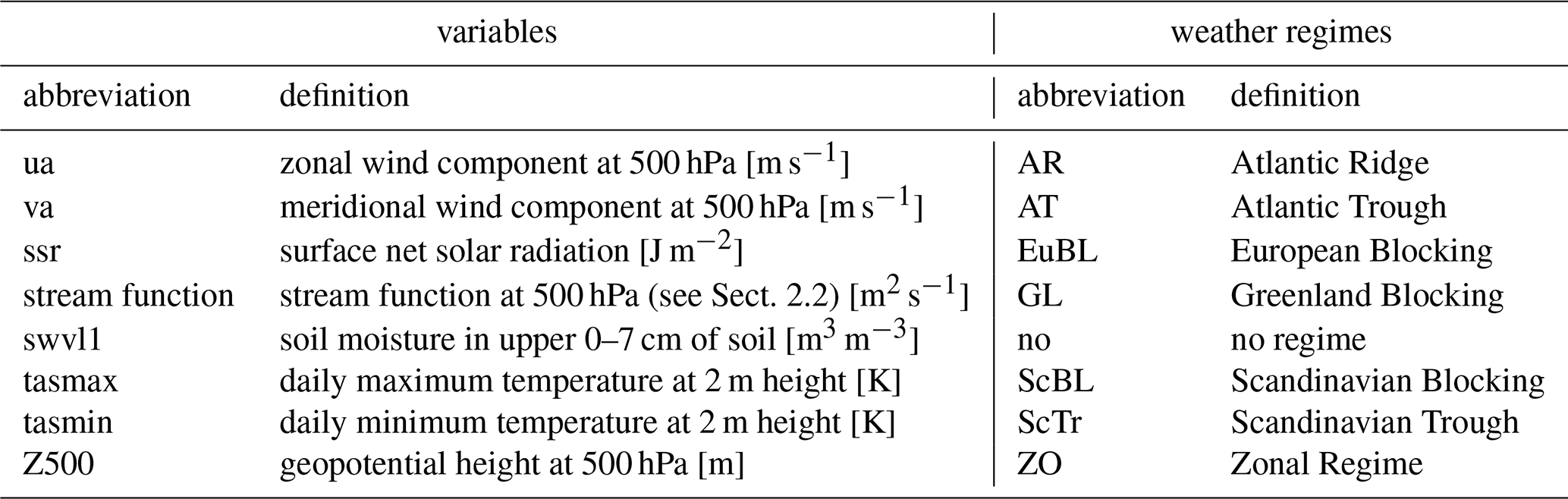
We use the ERA5 reanalysis dataset provided by the European Center for Medium-Range Weather Forecasts (ECMWF) for the period 1950–2023, as this is the period for which weather regime data are available. The considered variables are: maximum and minimum daily temperature (tasmax and tasmin), zonal and meridional wind components (ua, va) at 500 hPa, soil moisture content of the top layer in soil depth of 0–7 cm (swvl1) and surface net solar radiation (ssr), all at a spatial resolution of 0.5° and daily temporal resolution. Daily means were computed for all variables except tasmax and tasmin. Tasmax and tasmin were detrended linearly to remove long-term trends and seasonality in case of the dynamical system metrics. In practice, we used the Climate Data Operators (CDO) function detrend (Schulzweida, 2023). Anomalies for swvl, tasmax and Z500 were computed relative to a smoothed daily climatology using a 21-year running window mean. Anomalies of the dynamical system metrics were computed relative to their seasonal cycles (21d running window daily means). An overview over the utilized variables is given in Table 1. Our Euro-Atlantic domain for the large-scale atmospheric circulation (ua, uv) spans 15° W–30° E and 35–70° N (see solid black line in Fig. 1a). For better comparability with existing literature, heatwaves are defined in the Central Europe domain from 45–55° N and 4–16° E (red shading), analogous to Zschenderlein et al. (2019). Similarly, the near-surface variables are analyzed within a 40–60° N, 2–16° E domain (dashed line) exclusively on land, to focus on the heat wave region, while still including a sufficient number of grid points for the calculation of the analogs resulting in the dynamical system metrics. A sensitivity study of the chosen domains can be found in Appendix C.

Table 1 Definition of utilized variables and weather regimes. The weather regimes are shown as spatial maps in Appendix A.

2.2 Stream function

In order to investigate the mid-tropospheric atmospheric circulation relevant for heatwaves, we use the stream function at 500 hPa. The stream function offers an advantage over geopotential height for analyzing large-scale atmospheric circulation as it is insensitive to tropospheric warming. In contrast, geopotential height increases with global warming, requiring additional procedures like detrending for an accurate analysis (Faranda et al., 2022; Noyelle et al., 2023). We calculate the stream function ψ(x,y) globally from the zonal and meridional wind components (u, v) at 500 hPa using the formula (Holton and Hakim, 2013):

$$\begin{array}{}\text{(1)}& u=-{\displaystyle \frac{\partial \mathit{\psi }}{\partial y}},v=+{\displaystyle \frac{\partial \mathit{\psi }}{\partial x}}\end{array}$$

In practice, we use CDO functions to first compute the divergence and vorticity from the horizontal wind components (−uv2dv), followed by the computation of the stream function (−dv2ps) (Schulzweida, 2023).

2.3 Heatwave definition

Heatwaves can be identified using various methods (Robinson, 2001; Perkins and Alexander, 2013; Becker et al., 2022). In this study, we define heatwaves using the HWMid index introduced by Russo et al. (2015). It is based on a daily varying threshold of daily maximum temperature, which enables the year-round detection of heatwaves. Precisely, for each gridcell, a heatwave is a period of at least three consecutive days, which exceeds the 90th percentile of the daily distribution of daily maximum temperatures, calculated for a 31 d window in the 1991–2020 reference period. Further, we define a regional heatwave for 45–55° N, 4–16° E by requiring at least 5 % of the area being a heatwave for at least 3 consecutive days. The resulting number of heatwaves per month is shown in Fig. 1. Following Brunner and Voigt (2024), who highlighted potential biases from long running-window intervals, we assessed the sensitivity of our results to shorter intervals and found them to remain robust with changes in heatwave days of <1 %.

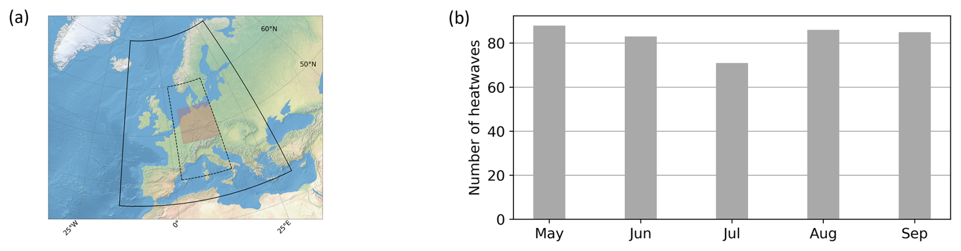
Figure 1 Utilized domains and heatwave statistics. (a) Domains for atmospheric circulation (solid box): 35–70° N, −15–30° E; (near-) surface variables (dashed box) 40–60° N, 2–16° E, used to compute the dynamical system metrics; and domain over which heatwaves are defined (red shaded box): 45–55° N, 4–16° E. (b) Number of defined heatwaves per month during 1950–2023. Heatwaves are considered in the month in which the majority of heatwave days occur. If the number of heatwave days is split equally between two months, the heatwave is considered in the start month.

2.4 Weather regimes

Weather regimes are helpful to characterize low-frequency variability of the large-scale atmospheric circulation. In this study, the year-round weather regime definition from Grams et al. (2017) is employed, which is based on standard approaches utilizing empirical orthogonal function analysis (EOF) and k-means clustering (Michelangeli et al., 1995; Michel and Rivière, 2011; Ferranti et al., 2015). The methodology is applied to the ERA5 dataset in the Atlantic-European region (80° W–40° E, 30–90° N) at a horizontal resolution of 1°. Geopotential height anomalies at 500 hPa are defined every six hours based on a 90 d running mean climatology from 1979–2019. Next, a 10 day low-pass filter is applied to exclude high-frequency signals. As the weather regimes are year-round, the seasonal cycle in the amplitude of the anomaly is removed by normalization with spatially averaged 30 d running window standard deviations. Then, the EOF analysis is conducted on the normalized Z500 anomalies. The leading seven EOFs, which account for 76.7 % of the variance, are employed for the k-means clustering. The resulting seven weather regimes (Appendix A) can be classified into three cyclonic regimes (Atlantic Trough (AT), Zonal regime (ZO), Scandinavian trough (ScTr)) and four blocked regimes (Atlantic Ridge (AR), European blocking (EuBL), Scandinavian Blocking (ScBL); Greenland Blocking (GL)). The ZO describes the positive and GL the negative phase of the North Atlantic Oscillation (NAO). Furthermore, the weather regime index I_wr (Michel and Rivière, 2011) is calculated to determine individual WR life cycles. It describes the projection of instantaneous Z500 anomalies to the cluster mean of the defined weather regimes. Thus, a high I_wr of one regime indicates that the instantaneous Z500 anomaly has a high similarity to the characteristic pattern of that specific weather regime. An active WR life cycle is defined as a period of at least five consecutive days during which I_wr >1, and during which a local maximum with a monotonic increase and decrease five days before and after is present. Subsequent life cycles of the same WR are merged if the mean I_wr is larger than 1 throughout the entire merged life cycle. In case that multiple WRs are in an active life cycle at the same time, the one with the highest I_wr is chosen as the active weather regime life cycle. It is also possible that no WR life cycle is active when the large-scale flow at a specific time does not meet the criteria. In such cases, its active weather regime life cycle is called no regime. Hereafter, the active weather regime life cycle will also be referred to as weather regime classification, occurrence, or category. Whenever I_wr is intended, this is explicitly stated. The WR definition based on 1979–2019 can be applied to times beyond this period, allowing the identification of the I_wr and WR life cycles for 11 January 1950–31 December 2023. However, as they are defined over 1979–2019, the relative frequency of the regime occurrence may change throughout the considered period 1950–2023 due to the natural decadal variability evident in various indexes e.g. the NAO and EA pattern (Pinto and Raible, 2012; Weisheimer et al., 2017). To align with the temporal resolution of the other variables used in this study, daily active weather regime life cycles are identified to represent the longest-lasting weather regime on any given day.

2.5 Persistence and co-recurrence calculation

To quantify the large-scale atmospheric circulation on heatwave days, as well as its link to other variables such as daily maximum temperature, the dynamical system metrics, persistence (θ⁻¹) and co-recurrence ratio (α), are computed. The persistence (Faranda et al., 2017b; Messori et al., 2017), describes the the tendency of e.g. an instantaneous atmospheric circulation pattern to remain similar to itself, while the co-recurrence ratio (Faranda et al., 2020) provides information about the instantaneous linkage of several variables. Both quantities have already been applied to a variety of reanalysis and model data (De Luca et al., 2020; Faranda et al., 2017a, 2020; Messori and Faranda, 2023; Holmberg et al., 2023; Faranda et al., 2024). The quantities are based on the concept of analogues, meaning a set of similar states of one variable, e.g. a set of similar atmospheric circulations. They should be identified for the absolute variables rather than anomalies. The reason is to ensure truly similar states. For instance, analogues of temperature anomalies could occur in different seasons with very different absolute temperatures, which would not be desirable. Analogues are found by comparing the states of one variable at all timesteps throughout the considered time period, with a reference state of the variable at a specific timestep. Thus, the variable of interest has a varying set of analogues per timestep. More precisely, the analogues (also referred to as Poincaré recurrences) are computed as follows:

1. The Euclidean distance is calculated between maps of the variable of interest for each timestep and those maps for all other timesteps in the dataset

2. Of these distances, the smallest 2 % (q=0.98) are selected as analogues, following De Luca et al. (2020); Faranda et al. (2020); Messori and Faranda (2023). This choice of quantile strikes a balance between a sufficiently large sample size and reasonably close analogues. Tests indicated minimal sensitivity of the results within the range $\mathrm{0.95}<q<\mathrm{0.99}$ (Faranda et al., 2017b). In our case, this corresponds to 541 analogues per day, representing 541 similar states for each day over the period 1950–2023. Among those analogues, the most frequent active weather regime life cycle consistently matches that on the reference day, indicating a good quality of the analogues.

As the co-recurrence ratio is defined only for multiple variables, the analogues for each variable are first retrieved separately. The extent of co-recurrence among analogues is then quantified by calculating, for each timestep, the number of analogues of all considered variables that occur on the same day in the dataset. This value is then normalized by dividing it by the total daily number of analogues for any variable. The obtained $\mathrm{0}\le \mathit{\alpha }\le \mathrm{1}$ reflects the strength of the relationship between the variables: a high α indicates strong linkage, while a low α suggests weak linkage. For instance, a high α between temperature and atmospheric circulation on a given day implies that similar temperature and circulation patterns frequently co-occur throughout the entire time series. It is important to note that α does not imply causality, as the result remains unchanged if the variables are swapped. However, since a link suggests the presence of shared underlying dynamics, α provides insights into the physical system under investigation. A high persistence θ⁻¹ can be intuitively understood as the variable of interest (e.g. the atmospheric circulation) remaining in a similar state for an extended period of time. It is an estimate for the average number of consecutive recurrences and can be thought of a cluster of analogues in time. Technically, θ⁻¹ is estimated using the algorithm of Süveges (2007). θ is known as extremal index and provides the inverse of persistence in units of the timestep of the data being analyzed. As $\mathrm{0}\le \mathit{\theta }\le \mathrm{1}$, if the inverse persistence θ is high, then the persistence is low and the variable will vary quickly. It has been shown that θ is related to the intrinsic predictability (Messori et al., 2017) of the atmosphere and may provide valuable information for the practical prediction of temperature (Holmberg et al., 2024). In this study, the inverse persistence θ⁻¹ of the atmospheric circulation is computed to analyze heatwave days, and the co-recurrence α will be primarily applied to identify the link between the atmospheric circulation and daily maximum temperature, but will also be applied to other variables. Both quantities are computed with the Chaotic Dynamical System Kit (CDSK) package (Robin, 2021).

3 Case study and seasonal cycles

Europe was affected by several heat waves between 20180–2022 with recurrent drought and strong legacy effects (Knutzen et al., 2025). To demonstrate the applicability of the inverse persistence and co-recurrence ratio in combination with weather regimes, we first examine the case study of the Central European heatwave of July 2019 (Sousa et al., 2020; Vautard et al., 2020; Klimiuk et al., 2025). This exceptional heatwave resulted in numerous records being broken, in particular in France, Belgium and the Netherlands (Sousa et al., 2020).

The dynamical evolution of the heatwave is illustrated in Fig. 2 by means of 500 hPa streamlines averaged over 5 d periods one week before prior to HW onset (Fig. 2a) and around its peak (Fig. 2b). Over the period 17–21 July, the large-scale flow setup over the Euro-Atlantic sector displayed no notable anomalies. Europe was still influenced by a weakening and eastward-moving long-wave trough, whereas the Atlantic region was characterized by zonal westerly flow. Overall, the large-scale circulation was rather close to summer climatology, which is further demonstrated in Fig. 2e, showing no anomalously elevated I_wrs for any regime during that period. In line with the large-scale flow, near-surface temperatures were close to summer climatology across the whole of Europe. The large-scale flow situation changed around 22 July when warm air advection ahead of two cyclones over the North Atlantic led to a rapid increase of geopotential heights over Europe. Over the next two days, the further amplification of the ridge over Europe resulted in the formation of an atmospheric blocking in the shape of an Omega (See Appendix D).

Large areas of western and central Europe were now experiencing temperature anomalies of more than 10K as visualized in Fig. 2d. At the same time, the soils begin to desiccate considerably. These dry conditions were preceded by soil moisture deficits in Central Europe (Fig. 2c), initiated by a heatwave at the end of June 2019. The pre-existing deficits significantly contributed to the intensity of the July 2019 heatwave. (Sousa et al., 2020; Knutzen et al., 2025)

Finally, Fig. 2f illustrates the temporal evolution of the July 2019 heatwave from the dynamical system metrics perspective. From the 18 July onward, the inverse persistence of the 500 hPa stream function starts to decline, reaching a minimum around the 26 July. This coincides very well with the peak development of the Omega blocking, which is a large-scale flow anomaly known to be rather persistent. Moreover, the onset phase of the heatwave is marked by a sharp increase in the co-reccurrence ratio, which underlines in this case the substantial linkage between the large-scale flow and near-surface temperature. We hypothesize that the subsequent decrease in the co-recurrence ratio around the 25 July likely reflects less common atmospheric dynamics with the I_wr of EuBL, and later GL, also exceeding 1 and/or the exceptionally high I_wr values of ScBL. This could explain the reduced frequency with which this atmospheric circulation and its corresponding temperature pattern occur simultaneously throughout the time series. In summary, this case study suggests that inverse persistence and co-recurrence may be linked to weather regimes and, therefore, yield physically meaningful insights, while co-recurrence may also provide valuable information on the relationship between atmospheric circulation and other variables.

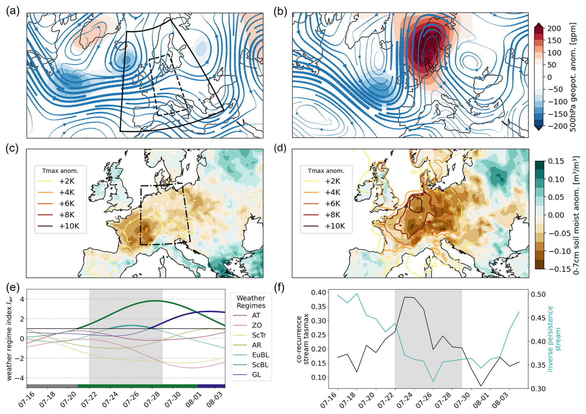
Figure 2 Case study of July 2019 heatwave. The spatial plots (a) and (b) depict the 500 hPa stream function and geopotential height anomalies, while (c) and (d) show soil moisture and daily maximum temperature anomalies. (a) and (c) show the mean over 17–21 July 2019 before the heatwave, while (b) and (d) show the peak heatwave mean over 23–27 July 2019. (a) also illustrates the domains over which the dynamical system metrics are computed (solid: stream function, dashed: tasmax), and (c) shows the heatwave domain. (e) illustrates the evolution of the I_wr index and the active weather regime life cycle at the bottom. Significance (I_wr>1) is indicated in bold, and the heatwave days are shaded in grey. (f) evolution of co-recurrence ratio between tasmax and stream function at 500 hPa and the inverse persistence of the stream function, heatwave days shaded.

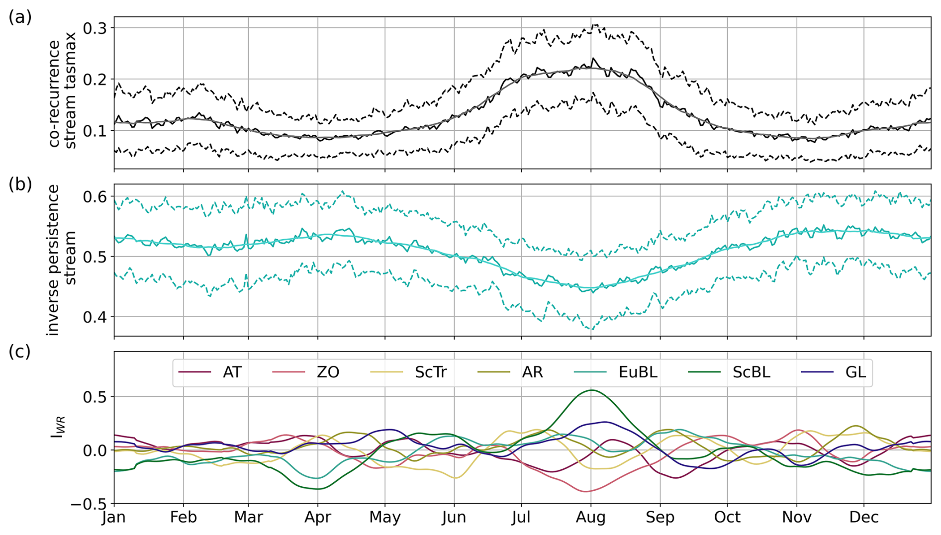
Figure 3 Strong seasonal variance in persistence of stream function and link between stream function and tasmax, and weather regime occurrence. Daily mean and std (dashed) over 1950–2023 with smoothed climatology (21 d running window, lighter color) of: (a) co-recurrence ratio of stream function and tasmax and (b) inverse persistence of stream function and (c) mean I_wr (only smoothed climatology) indicating which weather regimes govern the atmospheric circulation patterns of the respective days.

We now assess the characteristics of heatwaves across the entire historical period from 1950 to 2023. Given our focus on heatwaves from early to late summer, understanding the seasonal cycle of inverse persistence and co-recurrence is crucial for two reasons: first, to establish a baseline understanding of general seasonal variability, and second, to enable the identification of anomalies relative to this seasonal cycle. Figure 3 displays the daily mean across the entire time series, along with its standard deviation (dashed line) and a 21 d running window mean (lighter curve), for both the co-recurrence ratio between stream function and tasmax (Fig. 3a), and the inverse persistence of the stream function (Fig. 3b). The seasonal cycle of the co-recurrence ratio reveals a peak in July and August and a second smaller peak in January, with minima in April and November. The inverse persistence follows a similar seasonal cycle, with atmospheric circulation highly persistent during the summer months, while November and April exhibit the least persistent atmospheric circulation. Considering the extended summer months May to September, it is remarkable that the dynamical system metric values in the end of September are similar to the ones in the beginning of May, while the commonly considered summer months, June to August, display significantly lower values of both persistence and co-recurrence ratio in the beginning of June compared to end of August. This supports the use of the extended summer months as a more representative period of summer climatology. Anomalies of co-recurrence and persistence relative to their seasonal cycles will be examined in Fig. 5 for the extended summer months. To interpret those seasonal cycles, Fig. 3c displays the 21 d running window mean I_wr of all seven weather regimes. It becomes apparent that the high persistence of the atmospheric circulation in July and August coincides with a maximum in I_wr of the blockings ScBL, GL, and relative minima in the cyclonic regime ZO. Typically, the regions under atmospheric blocking experience only little advection, as the atmospheric circulation and the temperature patterns are mostly in phase (Tuel and Martius, 2024; Röthlisberger and Papritz, 2023b) and similar patterns in geopotential anomalies should therefore often result in similar patterns in temperature anomalies. Thus, we hypothesize that the more frequent occurrence of persistent blockings in summer might be associated with the summer peak in co-recurrence between temperature and stream function.

In addition to the pronounced peak summer months characteristics, Fig. 3 reveals the intra-seasonal variations during the extended summer months May to September. In September, the atmospheric circulation differs significantly from the peak summer months. Cyclonic regimes become more prevalent again during September and the blocking regimes GL and ScBL no longer exhibit an elevated frequency. From a dynamical system metric perspective, the overall atmospheric circulation during September becomes less persistent and the temperature and atmospheric circulation patterns are less likely to occur together. The dynamical system metrics at the beginning of May display similar values than in the end of September. However, the I_wr shows that different weather patterns are dominant in May and September. In May, until mid/end May, ScBL and GL are together with AT the dominant regimes, like in August, while those three regimes are minimal in September. Mid May until mid June is quite variable in the prevalence of the regimes. EuBL becomes dominant while GL loses some of its importance and ScTr and AT has a minimum. Interestingly, from mid June until July, a peak in zonal regime and ScTr appears while the other regimes have mostly minima. However, the atmospheric circulation overall becomes more persistent and has a higher co-recurrence.

In summary, the analysis highlights the necessity of considering May to September to fully capture the summer peak of co-recurrence and persistence. The I_wr reveals notable differences in dominant weather regimes both across and within months, demonstrating the benefit of combining weather regimes with dynamical system metrics. Consequently, those methods will be applied to heatwaves in the extended summer months (May–September) in the next analysis.

4 Characteristics of Heatwaves in the extended summer months

To investigate the characteristics of heatwaves and identify systematic differences in co-recurrence and inverse persistence compared to the summer climatology, we analyze heatwave days and non-heatwave days separately during the extended summer months. Figure 4a, b displays daily means of co-recurrence between stream function and tasmax, and of inverse persistence of stream function on heatwave days and non-heatwave days, with their corresponding standard error to account for the varying number of days considered. The co-recurrence of tasmax and stream function shows anomalously high values on heatwave days compared to non-heatwave days from the end of May to mid-September. For most days from the end of May to mid-September, the differences are statistically significant. Further, the magnitude of the difference is approximately constant over the significant part, except for a slightly lower anomaly in June. The findings are robust against the choice of domain (Appendix C). Interestingly, the anomalies of the inverse persistence of stream function show a different pattern than the co-recurrence ratio. A significantly higher persistence of the atmospheric circulation relative to non-heatwave days is only observed for a few scattered days from the end of June to the beginning of September. The differences between heatwave and non heatwave days are further less pronounced than for the co-recurrence ratio. This supports the findings of Holmberg et al. (2023), which suggest that the persistence of the large-scale atmospheric circulation is not a necessary criterion for the appearance of heatwaves in Europe. Moreover, our results reveal that only in July and August does the average atmospheric circulation associated with Central European heatwaves exhibit slightly increased persistence relative to non-heatwave days. We further report that those anomalies enhance for a smaller domain and vanish for a larger domain with a similar size than Holmberg et al. (2023), highlighting the importance of choosing a suitable region for the specific use case (Appendix C). In conclusion, heatwaves are characterized by an anomalous high co-recurrence ratio between tasmax and stream function end of May to mid-September, while a higher persistence of atmospheric circulation is only present in July and August. Therefore, a higher persistence of the atmospheric circulation does not necessarily lead to more similar temperature and stream function patterns.

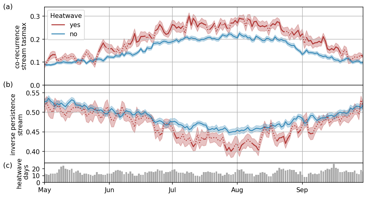
Figure 4 Comparison of heatwave and non heatwave days from May to September. Shown are daily means (lines) with corresponding standard error (shading) for (a) the co-recurrence ratio between stream function at 500 hPa and the daily maximum temperature and (b) for the inverse persistence of the stream function. Continuous lines indicate a statistically significant difference between heatwave and non-heatwave days according to a two-tailed bootstrap test at the 5 % significance level. (c) shows the daily number of heatwave days.

This finding is examined in more detail in Fig. 5, which presents a monthly breakdown (rows) of co-recurrence and persistence anomalies relative to their seasonal cycles (Fig. 3), combined with the corresponding weather regimes and daily maximum temperature anomalies.

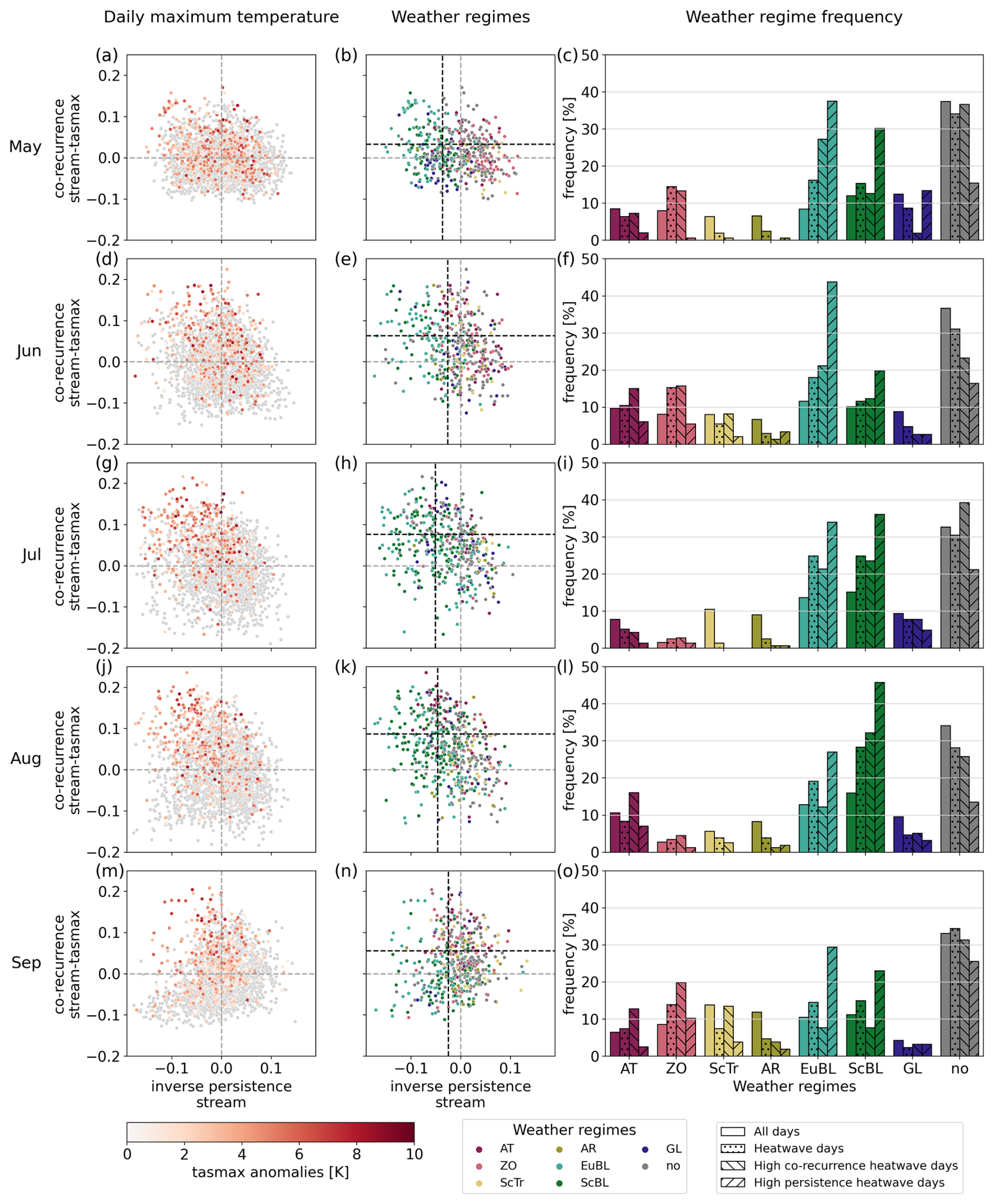
Figure 5 Relationship between weather regimes and dynamical system metrics during heatwaves throughout the summer season. Left column (a, d, g, j, m): Co-recurrence of stream function and daily maximum temperature anomalies on y axis and inverse persistence anomalies on the x axis from May to September (seasonal cycles of Fig. 3 subtracted). Each dot represents one day. Heatwave days colored in daily maximum temperature anomalies, no hw days shaded. Middle column (b, e, h, k, n): As left column, but colored in active weather regime life cycle on heatwave days. Upper tercile of co-recurrence and persistence dashed. Right column (c, f, i, l, o): Frequency of weather regime occurrence on heatwave days, on heatwave days with the highest co-recurrence anomalies (upper tercile) and on heatwave days with the highest persistence anomalies (lower tercile inverse persistence).

Starting with the first column, it becomes clear that most heatwave days (colored dots) are found in the upper half for all months and in the upper left quadrant in July and August (Fig. 5g, j) indicating anomalously high co-recurrence (vertical axis) and persistence (horizontal axis). This finding is in line with Fig. 4. Additionally, the highest tasmax anomalies (red colors) do not necessarily appear in clear clusters at specific persistent or co-recurrence anomalies. However, in August a strong tendency to the upper left quadrant can be observed (high co-recurrence, high persistence). July shows a similar pattern to August, but with a less pronounced concentration of strong heat anomalies in the upper-left quadrant. In September (Fig. 5m), a slight tendency of high tasmax anomalies on anomalous high co-recurrence values can be observed, but with a smaller anomaly in persistence. In contrast, the strongest tasmax anomalies in May (Fig. 5a) occur under less persistent atmospheric circulations, with no clear association to co-recurrence anomalies. In June (Fig. 5d), the strongest tasmax anomalies are either low persistent or highly persistent and with a positive co-recurrence anomaly (like in July and August). It thus reflects a transition from spring to peak summer. When considering all days instead of heatwave days, June, July and August (Fig. 5d, g, j) are similar in their overall distributions of anomalies in co-recurrence and inverse persistence. Those months have a oval shape with a slight tilted axis from upper left to lower right, suggesting some degree of correlation between co-recurrence and persistence. In contrast, September (Fig. 5m) has only few days in the upper left with a distance to the overall distribution, which distribution is tilted from bottom left to upper right. In May (Fig. 5a), in particular the co-recurrence has less low minimal values leading to the distribution being more densely packed. Thus, the degree of correlation between inverse persistence and co-recurrence differs in the extended summer months.

To relate the persistence and co-recurrence anomalies to the weather regimes, the second column of Fig. 5 shows all heatwave days colored in their active weather regime. It further indicates the monthly upper tercile of co-recurrence and lower tercile of inverse persistence on heatwave days (dashed black lines). The monthly values of the terciles reflect the findings of Fig. 4 that July and August are overall more persistent on heatwave days than in early and late summer and the co-recurrence anomaly on heatwave days is the highest in August, but varies only slightly from June to August.

Starting with May (Fig. 5b), the weather regimes appear clustered: the blocking regimes EuBL, ScBL, and GL lie on the left side, indicating higher persistence. GL is associated with low co-recurrence, while EuBL and ScBL show strong positive co-recurrence anomalies. In contrast, the more cyclonic regimes, ZO and AR, are less persistent and exhibit a wider range of co-recurrence anomalies. In June (Fig. 5e), these clusters become less distinct. EuBL and ScBL remain persistent, as observed consistently across all months, but the other regimes are more scattered, particularly across the full range of co-recurrence values. This pattern continues in July (Fig. 5h), although it's notable that most heatwave days occur under EuBL and ScBL, especially those with high co-recurrence and persistence (upper left quadrant). August (Fig. 5k) resembles July, but the AT regime becomes more frequent and also appears among the high co-recurrence, high persistence anomalies. In September (Fig. 5n), other regimes such as the ZO and AR become more frequent. However, the outliers with both high persistence and high co-recurrence values are primarily associated with EuBL and ScBL, while those with slightly lower persistence also include ZO.

The results show that heatwaves in the peak summer months, July and August, occur frequently under persistent blockings (EuBL, ScBL; Appendix B), while early and late summer heatwaves form under a greater variety of weather regimes. We detect a notably increased presence of the zonal regime and the “no regime” case for both May and September heatwaves. Despite those regimes excluding atmospheric blocking, they may still feature atmospheric ridges over Central Europe, and have been previously linked to heatwaves in the region (Lemburg and Fink, 2024).

Further, the weather regimes show tendencies for persistence anomalies, but vary greatly in their co-recurrence anomalies within and between the months. Considering the co-recurrence ratio of all months, it becomes apparent, that no particular regime(s) can be attributed to the anomalous high co-recurrence ratio on heatwave days.

To translate those qualitative findings into a quantitative result, we further considered the monthly weather regime frequency in panels c, f, i, j, o, comparing all days, heatwave days and heatwave days with the highest co-recurrence and lowest inverse persistence anomalies (terciles in the second column). In particular, we are aiming at answering the question which regimes dominate the persistence and co-recurrence anomalies on heatwave day and how the weather regime frequency at the most anomalous heatwave days differ from the weather regime frequency on heatwave days and all days.

First, the no regime category is the most frequent category on all days and particularly frequent during heatwave days with 28.2 %–34.2 % in every month. Interestingly, the no regime category occurs less often during the most persistent heatwaves days in every month, while it is more frequent in May and July (Fig. 5c, i) for the highest co-recurrence ratio heatwave days.

Then, the weather regimes most associated with heatwaves are EuBL, ScBL and ZO, as they are more frequent during heatwave days. EuBL (14.6 %–24.9 %) and ScBL (11.7 %–28.4 %) are particularly notable, as they are among the most frequent weather regimes in every month during heatwave days. In addition, these two regimes have increased occurrence during the most persistent heatwave days. Interestingly, EuBL shows a stronger frequency increase than ScBL on the most persistent heatwave days in May (Fig. 5c), June (Fig. 5c, f) and September (Fig. 5o). However, ScBL slightly exceeds EuBL in frequency above the heatwave average during peak summer (Fig. 5i, l). In terms of high co-recurrence ratio, EuBL is more frequent in May and June but declines in peak and late summer. ScBL shows fewer anomalies overall but is less common in May and especially in September with −7.3 percentage points. In contrast, the zonal regime, which is particularly common during early and late summer heatwaves, appears more often on high co-recurrence heatwave days in September (+6 %), but otherwise at similar frequencies as on average heatwave days. It is less persistent than the blockings and thus less frequent during high persistent heatwave days in all months. These differences point to the fact that the high persistent and high-co recurrent days are not necessarily coupled.

Considering the other weather regimes, all of them occur less frequently relative to heatwave days on the most persistent heatwave days except for GL in May and September. However, during the highest co-recurrence heatwave days AR is less frequent across all months. In early summer, GL is generally not associated with the most co-recurrent days. AT has an above-average heatwave day frequency on high co-recurrence heatwave days during June, August, and September (4.6 %–7.7 % percentage points), while ScTr occurs more frequently with 2.7 more percentage points in June and 6 more percentage points in September. This shows, that depending on the months, the weather regimes are more or less anomalous in co-recurrence, while they have tendencies for specific persistence values throughout all summer months.

5 The role of daily minimum temperature, soil moisture and solar radiation

As the anomalous high co-recurrence ratio on heatwave days cannot be attributed to specific weather regimes, we investigate the role of land-atmosphere interactions associated with heatwaves. Therefore, Fig. 6 depicts the co-recurrence ratio of tasmax and stream function at 500 hPa to daily minimum temperature (tasmin), soil moisture in the upper soil layer (0–7 cm (swvl1)) and surface net solar radiation (ssr). Conceptually Fig. 6 is similar to Fig. 4, showing daily means of heatwave and non heatwave days, as well as their standard error.

As the daily minimum temperature (tasmin) is related to radiation trapping during the night and has a large impact on perception of heat stress, its co-recurrence with tasmax and the stream function is analyzed. Figure 6a shows a high anomaly (Note the different y-scale) on heatwave days in July and August with a minor anomaly end of June. In September, tasmin and tasmax have a smaller co-recurrence ratio on heatwave days than on non heatwave days. During the core summer months, particularly warm days are expected to coincide with above-average nighttime temperatures due to limited time for nocturnal cooling, and the release of heat trapped during daytime. Consequently, patterns of maximum and minimum temperatures are closely linked, resulting in high co-recurrence values. However, later in the season, in September, day length decreases substantially, and areas experiencing high daytime temperatures may now tend to show average or even below-average nighttime temperatures, thus weakening the link between tasmax and tasmin. Additional factors might further influence nighttime radiative cooling, such as cloud cover and wind. The co-recurrence between stream function and tasmin (Fig. 6b) has a similar seasonal cycle, with statistically significant anomalies in July and August. However, the magnitude of the anomalies is highest end of July and in the beginning of August and drops faster than the co-recurrence anomalies between tasmin and tasmax. Moreover, no negative anomaly in September is observed.

Then, the link between soil moisture in the upper soil layer and tasmax is examined in Fig. 6c, as a lack of soil moisture availability can lead to more severe heatwaves, while high temperatures in turn also lead to a drying of soils. It shows an anomalous high link on heatwave days, which is particularly pronounced in July and the beginning of August. In general, from June to mid-September, there is a significantly higher linkage of soil moisture to temperature during heatwaves, while in May and in mid-to-late September, no significant anomaly is observed. A large intra-monthly variability of the co-recurrence can be observed, which could be associated with different spatial and temporal scales, as well as spatial heterogeneity. The link of soil moisture and stream function at 500 hPa (Fig. 6d) shows almost continuous statistically significant anomalies from mid-June to mid-September. This behavior is similar to the link of tasmax-swvl, but with an overall smaller magnitude and later start of the anomalies (mid June vs beginning of June). This indicates a high importance of soil moisture leading to heatwaves in particular in July and August. However, examining soil moisture availability prior to the heatwaves as a potential explanation for the high co-recurrence ratio anomalies between stream function and tasmax showed no clear link (Appendix E).

The co-recurrence between surface net solar radiation (difference between shortwave incoming and shortwave reflected radiation) and tasmax is assessed in Fig. 6e. On heatwave days, this link is anomalously high from May to August with particular high anomalies in June and July. As the solar radiation is strongest end of June, this might explain the observed asymmetry. The large anomalies are most likely attributable to the predominantly clear sky conditions associated with high pressure systems that mostly lead to heatwaves. This is confirmed by the co-recurrence between ssr and stream function (Fig. 6f), which shows a constant small anomaly on heatwave days during the extended summer months. Comparing the link between ssr and tasmax to the link between swvl and tasmax reveals that ssr is associated with a particular anomaly in early summer until mid August, while soil moisture shows the highest anomalies only in July and August. In addition, the surface net solar radiation is the only quantity which shows an anomaly on heatwave days in May, as the link between stream function and tasmax (Fig. 4) does not become anomalous until June. This indicates that heatwaves are driven by different processes and surface net solar radiation is particularly relevant for early summer heatwaves.

Thus, the surface net solar radiation on heatwave days is strongly related to daily maximum temperature in early summer, while soil moisture and temperature are strongly linked in July and August. However, the ssr has a constant link to atmospheric circulation at 500 hPa due to the predominantly clear sky conditions, while an anomaly in co-recurrence between soil moisture and stream function appears starting from mid June only. In addition, daily maximum and daily minimum temperatures are linked strongly in July and August, similar to daily minimum temperature and mid-tropospheric atmospheric circulation.

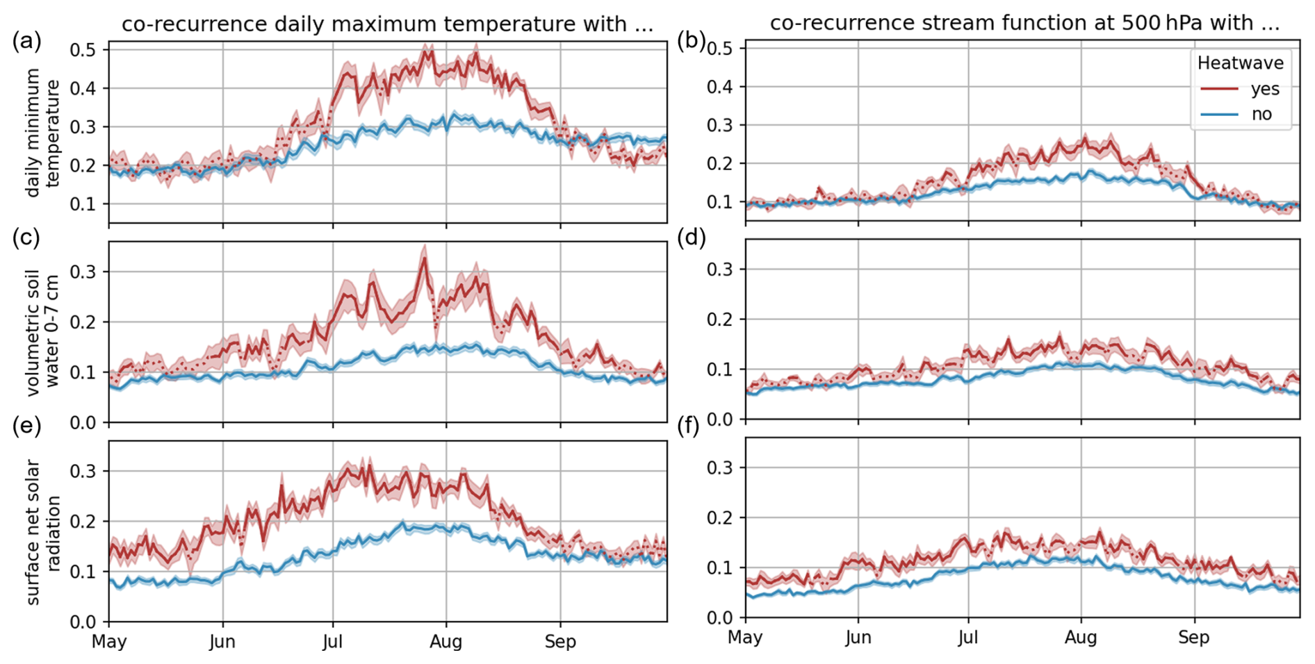
Figure 6 Comparison of the relationship between daily maximum temperature or stream function and daily minimum temperature, soil moisture during heatwave and non-heatwave days and surface net solar radiation. Daily mean co-recurrence ratio (lines) of (a, c, e) daily maximum temperature and (b, d, f) stream function to those variables on heatwave days vs on not heatwave days with standard errors shaded and non significance indicated by dotted lines.

6 Summary and concluding discussion

In this study we investigated the relationship between the large-scale atmospheric circulation and hot temperature extremes in Central Europe, with an emphasis on whether this relationship may also change throughout the summer season. With this aim, we used metrics derived from dynamical system theory, that allow both to objectively identify the persistence of any given atmospheric state and to further obtain an instantaneous measure of the association between two quantities. In addition, we use the concept of Euro-Atlantic weather regimes, which are physically meaningful modes of large-scale flow variability on subseasonal time scales. To exemplify the utilized methods, we first analyzed the July 2019 heatwave in Central Europe as a case study, followed by a climatological perspective. The main conclusions can be formulated as answers to our research questions as follows:

• How does the large-scale atmospheric flow and its link to surface temperature vary throughout the year?
  

  We find similar variations of both the co-recurrence ratio and atmospheric persistence throughout the year, with relative minima in spring and autumn and a maximum in July and August. Their high values in July and August are associated with an increased occurrence of Scandinavian blocking (ScBL) and reduced frequency of the zonal regime (ZO). While the inverse persistence and co-recurrence ratio display similar magnitudes in early and late summer, the dominant weather regimes differ. In May, the Scandinavian and Greenland blockings (ScBL, GL), as well as the Atlantic Trough (AT) dominate, while these are the least prevalent regimes in September. This highlights the added value of combining both approaches to better understand the atmospheric circulation – hot temperature link and capture the atmospheric dynamics even if the heatwaves are not associated with any regime.

• Is the atmospheric circulation more persistent on heatwave days, and is its link to surface temperature particularly high?
  

  We find a tendency for anomalously high values of atmospheric persistence on heatwave days only for the core summer months of July and August. In early and late summer, the atmospheric persistence is lower and indistinguishable from summer climatological values. Moreover, daily maximum temperature and the large-scale atmospheric circulation as characterized by the 500 hPa stream function show statistically significant anomalously high co-recurrence ratios on heatwave days from June to September, indicating an anomalous high link during heatwave days. Heatwave days with anomalously high persistence are attributable to the presence of blocking regimes over Europe. European and Scandinavian blockings are consistently overrepresented during highly persistent heatwaves across all summer months, with their occurrence peaking in July and August. The high co-recurrence ratio during heatwave days cannot be attributed to specific weather regimes, as their relevance varies between the months. For instance, heatwaves with a particularly strong link are often associated with European Blocking in early summer, while they are often associated with the zonal regime in September.

• How do soil moisture, surface net solar radiation and daily minimum temperature relate to daily maximum temperature on heatwave days?
  

  All three quantities show a distinct relationship to daily maximum temperature on heatwave days with different varying seasonal characteristics. Daily maximum temperatures over Central Europe exhibit a higher linkage to surface net solar radiation on heatwave days than on non-heatwave days from May to end of August, with maximum anomalies approximately aligning with the solar maximum in late June. The link of temperature to soil moisture anomalies is higher on heatwave days than on regular summer days with the exception of May and September. The strongest co-recurrence anomalies are observed towards late July and August. In addition, daily minimum and maximum temperature have an anomalously strong association in July and August compared to summer climatology. In September, the linkage drops below summer climatology, which is likely related to increasing nocturnal radiation cooling under clear skies.
  

Unlike previous studies (Faranda et al., 2020; De Luca et al., 2020; Holmberg et al., 2023), which characterized extreme events using dynamical system metrics, we combined persistence, co-recurrence ratio between various variables and weather regimes to gain a broader understanding of Central European heatwaves and their relationship to the large-scale atmospheric circulation. We further placed a strong emphasis on seasonal variations during the extended summer months, May to September. This focus is particularly interesting, given that Europe recently experienced severe heatwaves unusually late in summer/early autumn (Zschenderlein et al., 2018; Sun et al., 2025) and that projections from high-resolution climate models suggest that Central Europe may experience more frequent heatwaves particularly in late summer and early autumn in a warmer climate (Hundhausen et al., 2023). With this unique combination of methods, we provide a novel perspective on Central European heatwaves during the extended summer months.

Holmberg et al. (2023) have shown that mid-tropospheric atmospheric states with high persistence are not a necessary prerequisite for the emergence of hot extremes, neither in summer nor winter. Our results support and expand this finding for Central European heatwaves by considering the persistence and weather regimes on individual heatwave days during the extended summer months. For July and August, our results indicate a tendency for higher persistence on heatwave days due to the enhanced frequency of European and Scandinavian blockings. This finding supports the important role of blockings leading to heatwaves, which has been highlighted by several studies e.g. (Kautz et al., 2022). However, the size of this anomaly varies with the chosen domain size (Appendix C). In May, June and September, no persistence anomaly is observed, and cyclonic regimes such as the zonal regime are more frequent on heatwave days than in July and August.

Our finding that the co-recurrence ratio between tasmax and stream function at 500 hPa is anomalously high during heatwave days differs from the result of a study over North America examining the co-recurrence ratio between temperature and atmospheric circulation (Faranda et al., 2020). The authors concluded that summertime temperature extremes appear to be unrelated to joint dynamical properties in 2 m temperature and sea level pressure. However, our study differs from Faranda et al. (2020) not only in the considered region, but also in the considered variables. Instead of sea level pressure, we used mid-tropospheric stream function, as Holmberg et al. (2023) reported a weak relationship between summertime heatwaves and surface persistence, but rather a significant link to mid-tropospheric persistence. Moreover, we use daily maximum instead of daily mean 2 m temperature. In addition, both our domain for atmospheric circulation and for temperature are smaller than the ones in Faranda et al. (2020), as we aimed at targeting only the relevant features for heatwaves in Central Europe instead of covering the entire continent. The anomalous high link is however robust to changes in domain size (Appendix C).

In the last step of our study, we computed the co-recurrence ratio to assess the link between daily maximum temperature and soil moisture, daily minimum temperature and net surface solar radiation. Previously, De Luca et al. (2020) found an increasing co-recurrence ratio of daily precipitation and daily maximum temperature over the past 40 years in the Mediterranean, possibly associated with lower soil moisture in a warming climate. While we did not examine trends in our study, we found a strong link between soil moisture and daily maximum temperature in the summer months. Moreover, De Luca et al. (2020) did not find particular synoptic structures leading to the warm-dry extremes, hypothesizing that this is due to different sets of weather circulation regimes. This is in line with our results: For the co-recurrence ratio between stream function and daily maximum temperature, the highest anomalies on heatwave days are driven by different atmospheric flow fields, whose relative frequency further varies over the extended summer months.

While providing a novel perspective on heatwave dynamics, some limitations arise from the choices and properties inherent to the methods themselves. One choice is the size of the considered region for both co-recurrence and persistence. It determines how much the analogues resemble each other and should thus be chosen to match the specific use case. Nonetheless, our result of anomalous high co-recurrence ratio on heatwave days is robust against varying domain sizes (Appendix C), even though some sensitivity on the choice of model domain is found for the persistence. As the analogues are computed for daily data, some caution has to be applied when interpreting the co-recurrence ratio of slowly varying variables, such as soil moisture. However, this methodological characteristic is not expected to compromise the analysis of the other variables considered in this study or their relationship with temperature. Further, from the co-recurrence ratio between atmospheric circulation and temperature patterns, the role of advection cannot be directly inferred, as a high association between the two variables may occur both under advection-driven and non-advection-driven conditions. Additionally, to ensure a comparable number of analogues across decades, it is necessary first to remove the global warming trend. Otherwise, similar states in the past with slight differences in spatial distribution or magnitude may not be identified as analogues. While weather regimes allow a more intuitive understanding of the state of the large-scale atmospheric circulation, difficulties in interpretation can arise due to the frequent occurrence of the no regime category. The absence of a weather regime may result from a variety of atmospheric circulation patterns. For instance, the no regime phases may still feature short-lived atmospheric ridges, and thereby allow heatwave formation over Central Europe, as evidenced by our results showing comparable high frequencies of no regime for both heatwave and non-heatwave days.

Several open questions and future directions arise from this work. First, it would be valuable to extend the analysis to other heatwave domains in Europe to test the generality of the observed links. Second, investigating the full life cycle of heatwaves might reveal further characteristics. Third, to better capture the temporal dynamics and predictability, the recently developed local predictability index (Dong et al., 2025) could be applied. While we have not addressed the impacts of heatwaves, future work could also examine links to vulnerability, such as effects on agriculture (e.g., blooming or frost risk) and mortality. Lastly, evaluating how these relationships may shift under future climate conditions would provide essential insights into potentially changing atmospheric dynamics leading to heatwaves. This last step is planned as future work using CMIP6.

Appendix A: Weather regimes

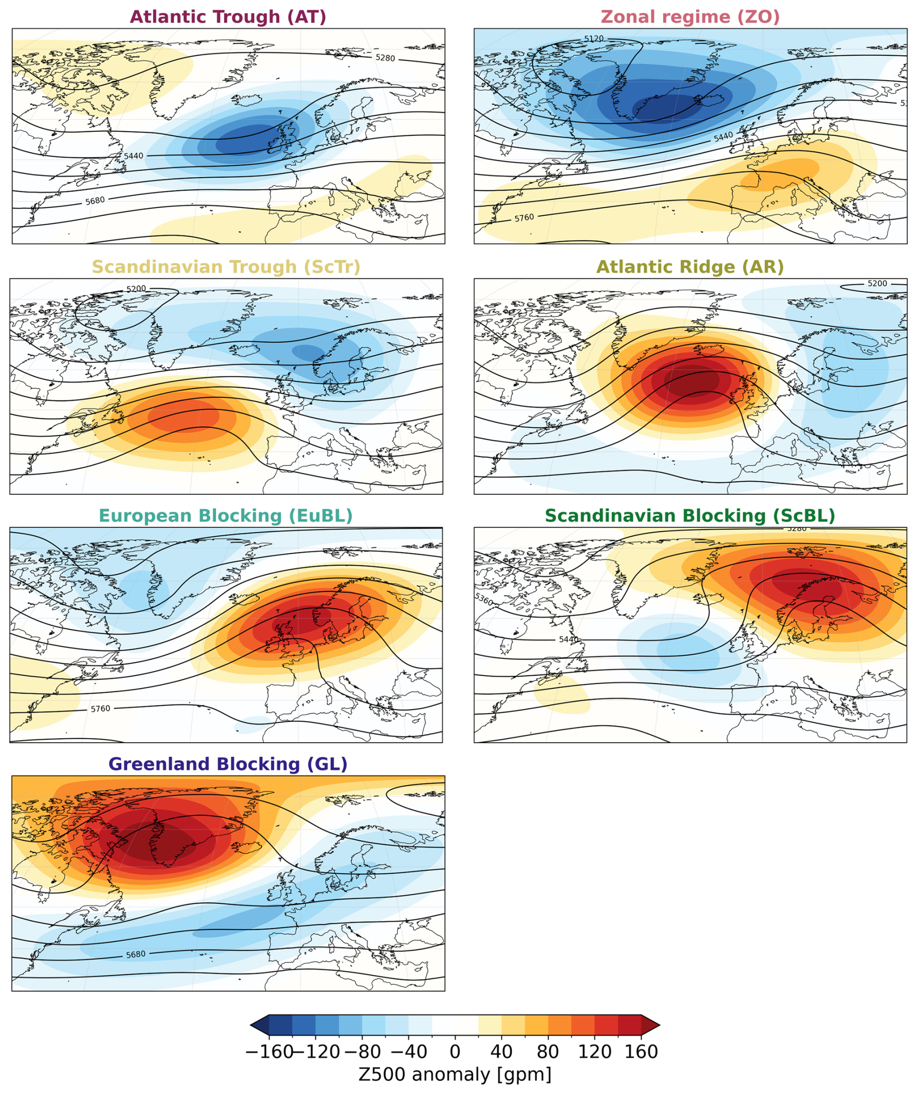
Figure A1 Mean 500 hPa geopotential height (contours; geopotential meters (gpm)) and corresponding anomalies (shading; gpm) of the seven year-round Atlantic–European weather regimes (Grams et al., 2017). Figure adapted from Osman et al. (2023), based on weather regimes defined by (Grams et al., 2017).

Appendix B: Average persistence values per weather regime

Figure B1 shows the distribution of inverse persistence per weather regime during May–September. It becomes apparent that EuBL and ScBL are the most persistent regimes, followed by GL, while the least persistent regimes are ZO and ScTr. The blocked weather regimes are thus more persistent than the cyclonic weather regimes.

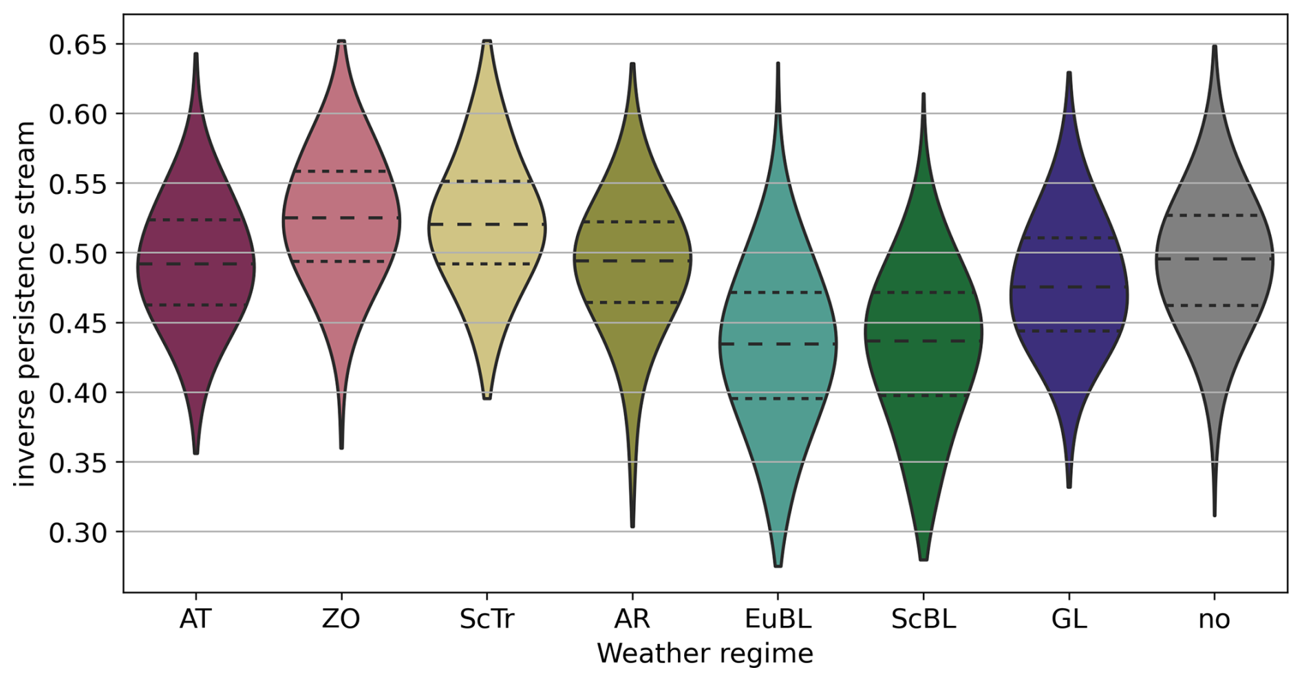
Figure B1 Distribution of inverse persistence of the weather regimes (active life cycle) during May–September in 35–70° N and −15–30° E.

Appendix C: Sensitivity Study Domains

We tested several domains for both stream function and daily maximum temperature as the choice of domains impacts how similar the analogues are. We find a robust higher co-recurrence ratio during almost all of the extended summer months. The inverse persistence varies with the varying domain size, highlighting the importance of choosing the domain suitable for the specific use cases.

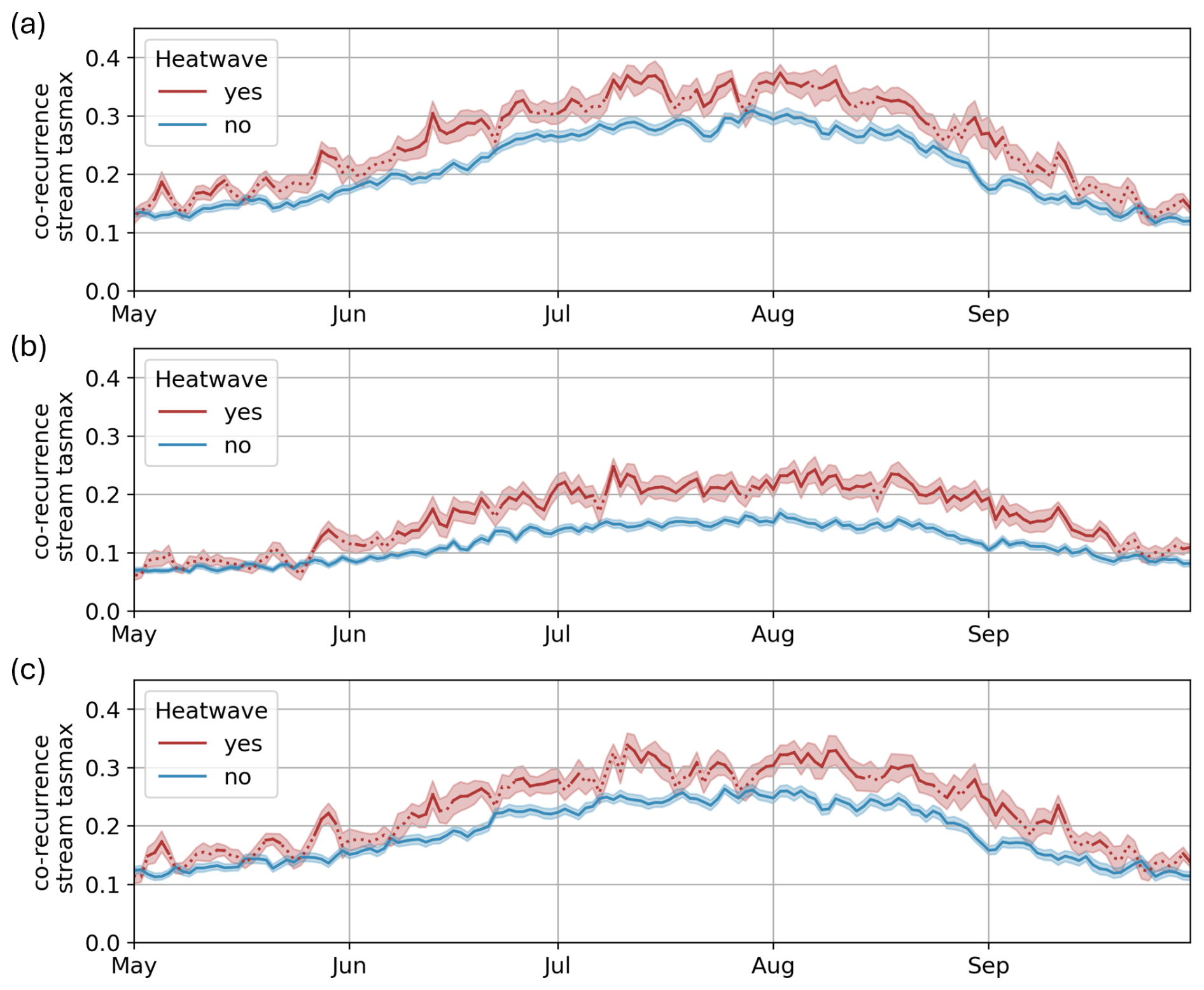
Figure C1 Co-recurrence ratio anomalies between tasmax and stream function for varying temperature domains. Daily mean co-recurrence ratio (lines) and standard error (shaded) on heatwave and non heatwave days for stream function in 35–70° N, −15–30° E and tasmax box (a) 35–70° N −15–30° E, (b) 45–55° N 4–16° E, (c) 40–60° N −10–25° E. Non statistical significance is indicated by dotted lines.

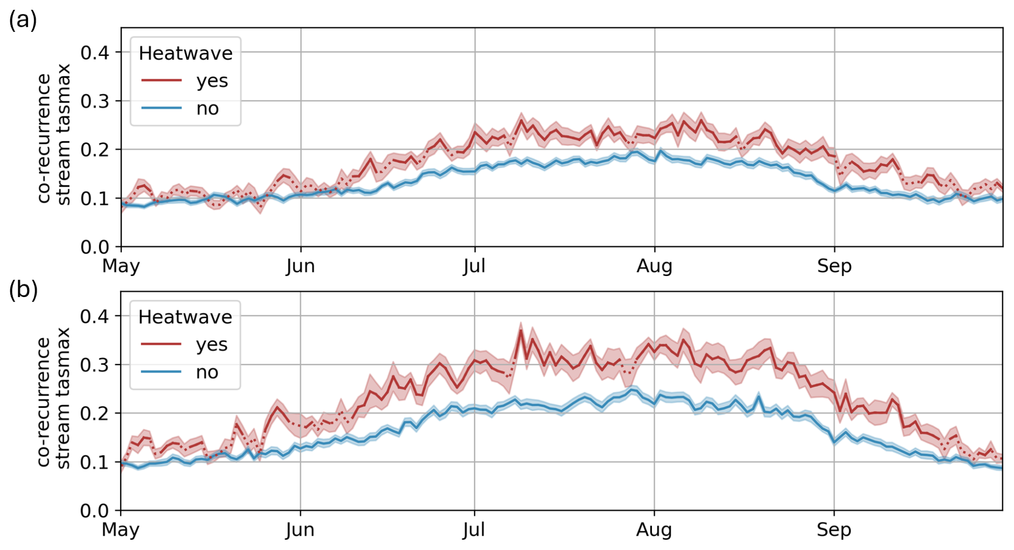
Figure C2 Co-recurrence ratio anomalies between tasmax and stream function for varying stream function domains. Daily mean co-recurrence ratio and standard error on heatwave and non heatwave days for tasmax in 40–60° N, 2–16° E and stream function box (a) 30–75° N −30–40° E, (b) 40–60° N 0–20° E. Non statistical significance is indicated by dotted lines.

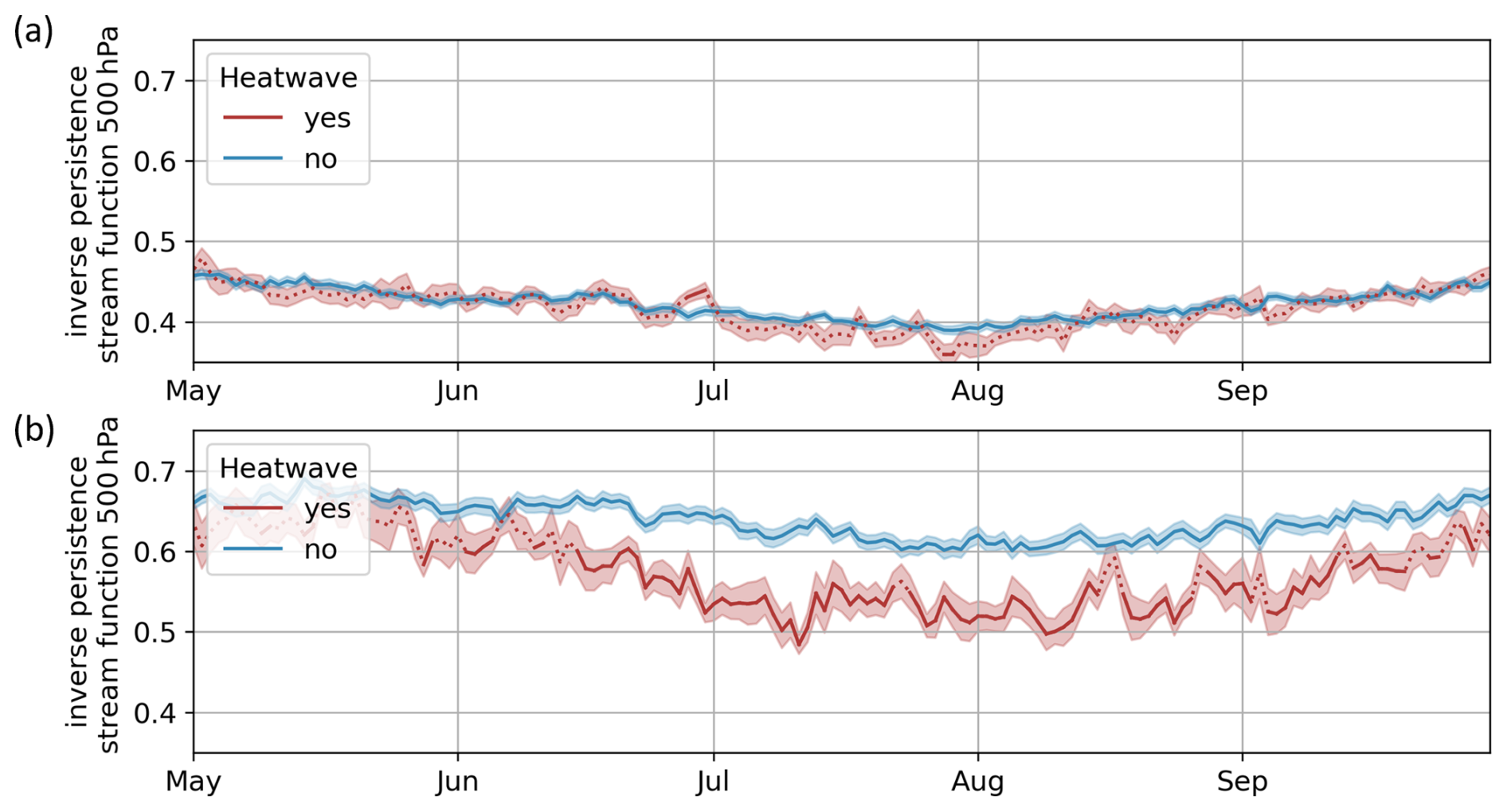
Figure C3 Inverse persistence anomalies of stream function for varying stream function domains. Daily mean inverse persistence and standard error on heatwave and non heatwave days for stream function in (a) 30–75° N, −30–40° E (b) 40–60° N 0–20° E. Non statistical significance is indicated by dotted lines.

Appendix D: Case Study

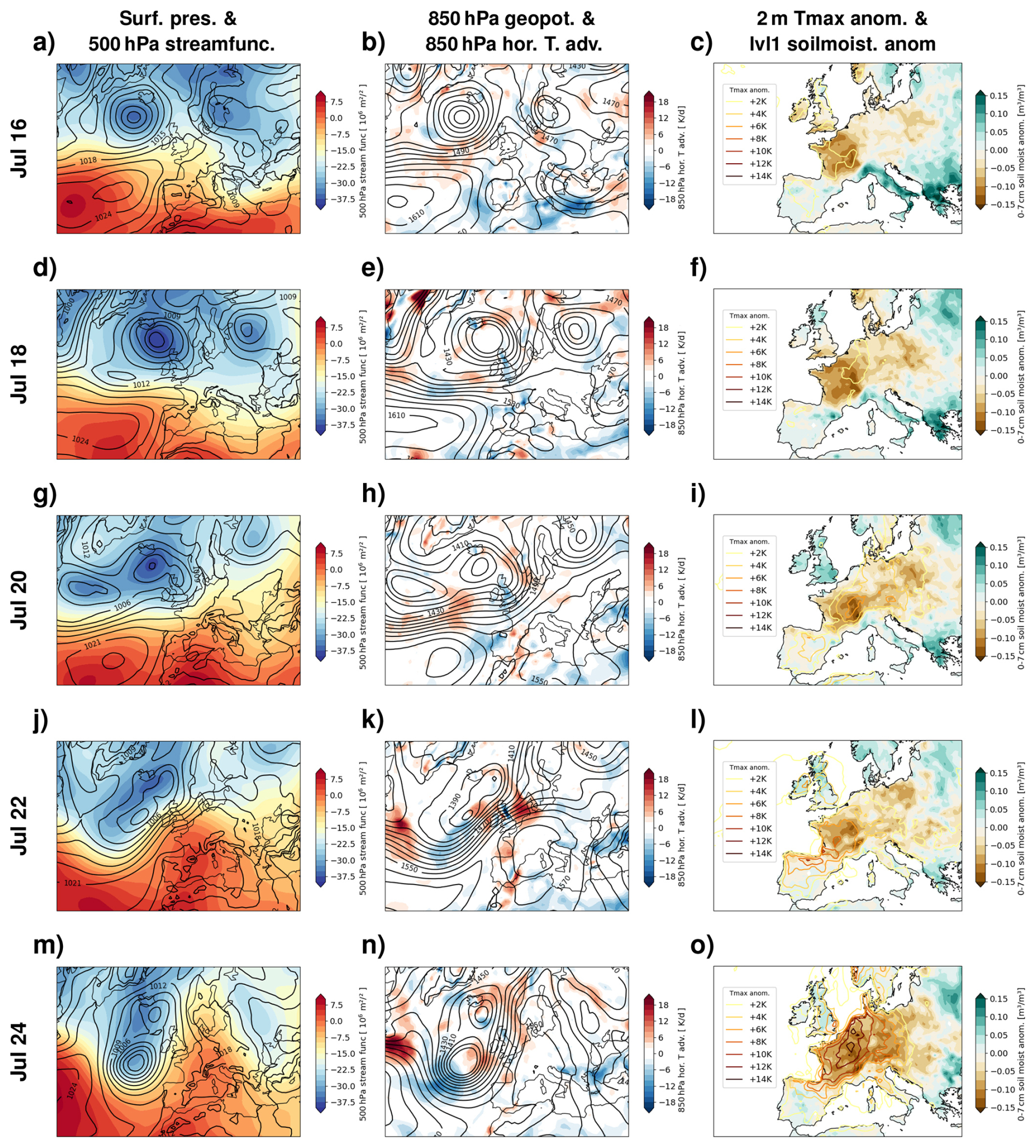
Figure D1 Case study of the July 2019 heatwave. For every second day starting on 16 July, we depict daily mean fields based on ERA5 data. Left column: Surface pressure (contours) and 500 hPa stream function derived from zonal and meridional wind fields (shadings). Middle column: Geopotential at 850 hPa (contours, as a proxy for the lower-tropospheric circulation) and 850 hPa horizontal temperature advection (shadings). Right column: 2 m maximum temperature anomalies and 0–7 cm soil moisture anomalies as in the main article.

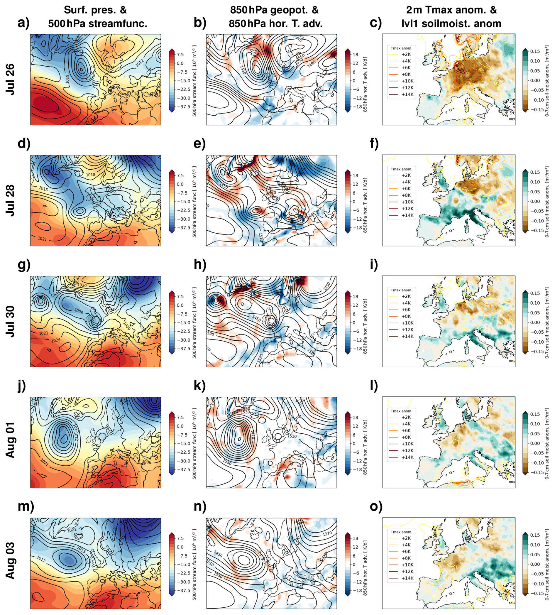
Figure D2 Case study of the July 2019 heatwave, continued.

Appendix E: Soil moisture

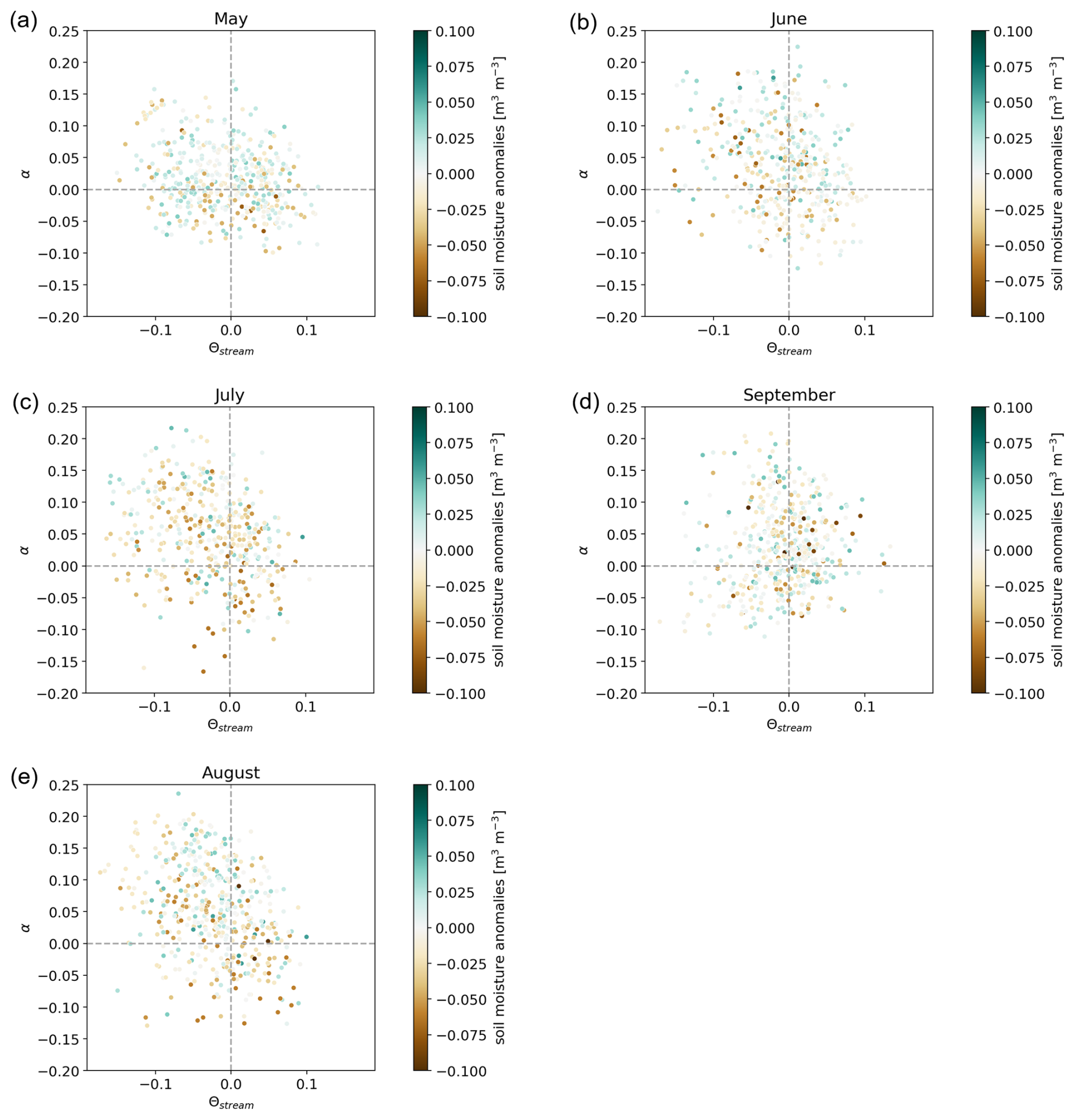
Figure E1 Persistence and co-recurrence anomalies cannot be clearly attributed to soil moisture anomalies prior to heatwaves. shown is co-recurrence ratio anomalies for stream function-tasmax (y-axis) and inverse persistence anomaly for stream function (x-axis). Each dot represents one heatwave day, colored in the average soil moisture anomalies in the week prior to the heatwave onset.