Exploring divergent long-term stratospheric aerosol injection scenarios with the G2-SAI and ARISE-hybrid experiments

Stratospheric aerosol injection (SAI) simulations are often short relative to climatic timescales and conducted against a background that evolves due to changes in anthropogenic greenhouse gas emissions and other forcings. This can cause challenges in assessing certain impacts of the intervention, especially for aspects of the climate that respond slowly to such changes. The early Geoengineering Model Intercomparison Project (GeoMIP) G2 experiment prescribes solar dimming to offset 1 % CO₂ forcing in a preindustrial control background. Here we propose a new G2-SAI experiment, in which SAI is applied in the same scenario, to isolate SAI climate responses from transient changes other than CO₂. Using the Community Earth System Model (CESM2), we present three 150-year “G2-SAI” simulations which use contemporary SAI strategies: two use the commonly-used “three degree-of-freedom” (“3DOF”) strategy, in which independent injections at 30° N, 15° N, 15° S, and 30° S are used to manage global mean temperature (T₀) and large-scale meridional temperature gradients (T₁, T₂). Our third G2-SAI simulation uses a “1DOF” strategy that injects at 30° N and 30° S to manage global mean temperature only. Our two 3DOF simulations both maintain the same temperature targets; however, one simulation, which injects mostly at 15° S, slows but does not prevent the decline of the Atlantic Meridional Overturning Circulation (AMOC) compared to the baseline simulation, while the other, which injects mostly at 30° N and 30° S, stops the decline of AMOC entirely, similarly to the 1DOF simulation. These results demonstrate that multiple distinct Earth system states can satisfy the same temperature targets, challenging the assumption of linearity commonly used in strategy design. In addition, the results highlight that long simulations are required to identify some of the long-term impacts of SAI, such as AMOC changes. Using this knowledge, we revisit the ARISE-SAI-1.5 experiment and modify the injection strategy without changing the temperature targets, producing an “ARISE-hybrid” ensemble. We demonstrate that this results in some significant differences in the climate response to SAI, with implications for the perceived effects of the intervention.

1 Introduction

Solar radiation modification (SRM), also known as climate intervention, climate engineering, or (solar) geoengineering, refers to a family of proposed interventions that would result in deliberate, large-scale modifications to the Earth system intended to reduce the impacts of global warming until greenhouse gas (GHG) concentrations can be stabilized. Stratospheric aerosol injection (SAI) – the deliberate increase of the stratospheric aerosol burden, which would cool the planet by reflecting a small portion of sunlight to space, similarly to what has been observed after larger volcanic eruptions (Budyko, 1977; Crutzen, 2006) – is perhaps the best understood of these proposed methods (Visioni et al., 2023b).

Much research into the physical science of SAI is conducted using climate model simulations, often coordinated through the Geoengineering Model Intercomparison Project, or GeoMIP (Kravitz et al., 2011). The first phase of GeoMIP experiments (“G1”, “G2”, “G3”, and “G4”) were highly idealized, with some (G1 and G2) protocols prescribing solar dimming and standardized idealized model scenarios such as pre-industrial (PI) control, 1 % CO₂ (annual 1 % increases in CO₂ concentrations) and abrupt 4×CO₂ (abrupt quadrupling of CO₂ concentrations). Other experiments included sulfur injections at the equator or in a fixed region in the tropics, or fixed aerosol fields (G3 and G4). As model complexity and understanding of SAI impacts have grown, more experiments (GeoMIP and non-GeoMIP) have incorporated policy-relevant future scenario projections, direct simulation of sulfur injection and oxidation, and more complex intervention strategies. Phase 6 of GeoMIP – so named to synchronize with Phase 6 of the Coupled Model Intercomparison Project, or CMIP6 (Eyring et al., 2016) – proposed the experiments G6sulfur and G6solar in 2015 (Kravitz et al., 2015), with the results published in 2021 (Visioni et al., 2021); these experiments prescribed near-equatorial SO₂ injection and globally uniform solar dimming, respectively, to reduce warming in a high-emissions CMIP scenario to levels of a medium-warming scenario. Meanwhile, MacMartin et al. (2017) and Kravitz et al. (2017) developed a strategy to simultaneously manage global mean temperature (“T₀”), interhemispheric temperature gradient (“T₁”), and equator-to-pole temperature gradient (“T₂”) with injections at four different latitudes (30° N, 15° N, 15° S, 30° S) in the Community Earth System Model version 1 (CESM1). This experiment, performed in a 20-member ensemble framework, formed the Geoengineering Large Ensemble, or GLENS (Tilmes et al., 2018). Since then, SAI strategy design has generally moved away from equatorial injection, with studies finding it tends to over-confine aerosols to the tropical pipe, over-cool the tropics and under-cool the poles, and drive substantial stratospheric heating perturbations and the resulting impacts on circulation (e.g., Bednarz et al., 2023; Henry et al., 2024), including the shutdown of the Quasi-Biennial Oscillation (QBO) (Aquila et al., 2014; Richter et al., 2017). In contrast, this “3 degree-of-freedom” (“3-DOF”) framework has since been used multiple times for SAI across models and model generations, including overshoot scenarios in CESM2 (Tilmes et al., 2020), scenario exploration in CESM2 (MacMartin et al., 2022), the standardized ARISE-SAI-1.5 experiment in CESM2 (Richter et al., 2022) and in UKESM1 (Henry et al., 2023), and the application to the G6sulfur scenario in UKESM1, which the authors called G6controller (Wells et al., 2024). The successor to the G6sulfur experiment, G6-1.5K-SAI, proposed in 2024 (Visioni et al., 2024) with preliminary results published in 2026 (Lee et al., 2026), uses 30° N and 30° S injection in equal amounts to manage global mean temperature, with the intention of striking a balance between experiment simplicity and optimality that incorporates the advances in strategy design informed by the earlier studies described above.

While scientific knowledge of the potential impacts of different SAI interventions has increased substantially over the past decade, significant uncertainties remain. Here, we focus on two characteristics that most contemporary SAI experiments share: firstly, they are often simulated against a backdrop of simultaneous changes based on commonly used climate change scenarios. GLENS used the Representative Concentration Pathway (van Vuuren et al., 2011) RCP8.5 scenario; G6sulfur and G6solar used the Shared Socioeconomic Pathway (O'Neill et al., 2016) SSP5-8.5 scenario; and ARISE-SAI-1.5 and the upcoming G6-1.5K-SAI use the moderate-warming SSP2-4.5 scenario, all of which are designed to project changes in the Earth system over the 21st century. Such a design choice thus includes not only the imposed changes from SAI but also transient changes from other climate forcings, tropospheric aerosols, and land use, which impose additional internal feedback. Even when directly comparing two otherwise identical simulations with and without SAI within a single model, it can sometimes be challenging to disentangle the impacts of the intervention from the feedbacks created by these multiple simultaneous changes. Furthermore, models and experiments disagree on the latitudinal distribution of injections needed to meet certain objectives; GLENS and ARISE-SAI-1.5 shared a similar design, but in the GLENS experiment (CESM1, RCP8.5 background), most of the SO₂ was injected into the Northern Hemisphere at 30° N, and in the ARISE-SAI-1.5 experiment (CESM2, SSP2-4.5 background), most of the SO₂ was injected into the Southern Hemisphere at 15° S. Fasullo and Richter (2023) proposed several hypotheses for the difference; while they could not positively identify the exact reasons for differing model behavior, they identified differences in fast cloud responses in different hemispheres due to model biases; differing behavior of the Atlantic Meridional Overturning Simulation (AMOC), which transports warm water poleward and deeper cold water equatorward; and differences in radiative forcing due to changes in tropospheric aerosol concentrations and their contributors. When ARISE-SAI-1.5 was conducted in UKESM1 (Henry et al., 2023), it required different injection locations (mostly 30° N and S) than CESM2 (mostly 15° S) to meet its own T₀–T₁–T₂ targets. In G6-1.5K-SAI, (equal amounts 30° N and S injection), CESM2 overcools the Northern Hemisphere, E3SMv3 cools both hemispheres relatively evenly, and MIROC-ES2H and UKESM1.1 have significant residual Arctic warming. Differences in the behavior between models remain poorly understood and may be related to different climate model sensitivities to both GHG and aerosol forcings and differences in aerosol transport.

Secondly, most SAI simulations are relatively short compared to climatic timescales. This follows in part from the first characteristic, as simulations of future scenarios such as the SSPs are often available only through model year 2100 (for example, O'Neill et al., 2016, defines CMIP6 ScenarioMIP simulations beyond 2100 as “long-term extensions” that are neither Tier 1 nor Tier 2). Additionally, modeling experiments often prescribe a “plausible” start date in the “near future” (at the time of publication); together, these constrain both the start and end dates of the simulated experiment. Computation time for a fully-coupled ESM is expensive, and some protocols choose to further shorten the experiment to produce more ensemble members instead. Lastly, future projections of global warming (and the impacts of SAI in those future states) become increasingly uncertain as they move further away from the present day. GLENS and G6sulfur run for 80 model years, ARISE-SAI-1.5 runs for 35 years, and G6-1.5K-SAI runs for 50 years. As a result, some impacts of SAI can be more difficult to evaluate in those simulations, in particular those that involve feedbacks with the more slowly changing ocean circulation, such as the AMOC.

To aid in exploring these uncertainties, we revisit the more idealized G2 experiment originally proposed by GeoMIP in 2011. G2 prescribed decreases in the solar constant to offset the forcing from annual 1 % increases in CO₂ (“1 % CO₂” forcing) for 50 years against a PI control background. Such designs include no other changes in anthropogenic forcings beyond the gradual CO₂ increase and no prior imposed long-term warming trends in naturally varying systems such as the AMOC, making them ideal for testing model behavior and feedback. Here we conduct three similar “G2-SAI” experiments in CESM2, utilizing the fully-coupled model and directly simulating the injection of SO₂ as well as extending the simulation length to 150 years. We design injection strategies to incorporate scientific advances made since the original G2 experiment was proposed and mirror other contemporary experiments. Two of our simulations utilize the 3-DOF, T₀–T₁–T₂ framework, and our third experiment uses hemispherically symmetric injection to manage global mean temperature only, as in G6-1.5K-SAI. We present our experimental setup in Sect. 2, the results of the G2-SAI experiments in Sect. 3, implications for the ARISE-SAI-1.5 in Sect. 4, and conclusions in Sect. 5.

2 Methods

2.1 Climate Model

The Community Earth System Model, version 2 (CESM2), is a state-of-the-art Earth system model developed by the U.S. National Science Foundation's National Center for Atmospheric Research. We run the model with fully-coupled atmosphere, land, ocean, sea ice, land ice, and river runoff components. For the atmosphere component, we use the Whole Atmosphere Community Climate Model (WACCM6, Gettelman et al., 2019); this configuration, CESM2(WACCM6), contributed to Phase 6 of CMIP (Eyring et al., 2016) and Phase 6 of GeoMIP (Visioni et al., 2021) and has been used extensively to model SAI (e.g., Tilmes et al., 2020; Richter et al., 2022; MacMartin et al., 2022; Lee et al., 2026). We run the model with a horizontal resolution of 0.9° latitude by 1.25° longitude, and WACCM6 uses 70 vertical layers with a model top at approximately 140 km ($\mathrm{4.5}\times {\mathrm{10}}^{-\mathrm{6}}$ hPa). This configuration includes comprehensive tropospheric, stratospheric, mesospheric and lower thermospheric (“TSMLT”) chemistry and prognostic aerosol physics and chemistry using the Modal Aerosol Module (MAM4, Liu et al., 2016), which includes Aitken, accumulation, and coarse mode representation for sulfate aerosols, with some modifications to modal size distributions introduced by Mills et al. (2016). For the ocean component, we use the Parallel Ocean Program version 2 (POP2, Smith et al., 2010; Danabasoglu et al., 2012, 2020), and for the land component, we use the Community Land Model version 5 (CLM5, Lawrence et al., 2019).

All of the simulations described in the next section (novel, and previously published) use this same configuration. For simulations with SAI, the SAI is implemented by placing SO₂ directly into a gridbox at pre-defined latitudes, approximately 5 km above the tropopause.

2.2 Simulation description

In this portion of the study, we consider nine CESM2 experiments: four simulations of scenarios without SAI (all previously published elsewhere), and five simulations of SAI (two previously published, and three novel). These simulations are summarized in Table 1 below.

The four no-SAI simulations are PI control, 1 % CO₂, Historical, and SSP2-4.5. PI control refers to the 500-year CMIP6 preindustrial control simulation. 1 % CO₂ is a CMIP6 GHG forcing scenario, branching from year 70 of the PI control simulation, in which CO₂ concentrations increase by 1 % annually. Historical refers to CMIP6 simulations of the 1850-2014 historical period. SSP2-4.5, part of the Shared Socioeconomic Pathway framework used in CMIP6 (O'Neill et al., 2016), is a moderate warming, “middle-of-the-road” projection of future climate change in which emissions do not deviate substantially from historical trends. The SSP2-4.5 simulations considered here begin in model year 2015, branching from Historical, with five ensemble members running until 2100 and the other five running until 2070.

The two previously-published SAI simulations we analyze are ARISE-SAI-1.5 (Richter et al., 2022) and G6-1.5K-SAI (Visioni et al., 2024; Lee et al., 2026); both branch from the SSP2-4.5 emissions scenario in model year 2035 and use SAI to maintain reference period temperatures corresponding to the 2020–2039 SSP2-4.5 average. G6-1.5K-SAI injects at 30° N and 30° S in equal quantities, with injection amounts chosen using a feedback algorithm (described below) to maintain global mean temperature (T₀) only; ARISE-SAI-1.5 injects at four latitudes (30° N, 15° N, 15° S, and 30° S) in different quantities, using a more complex feedback algorithm to manage not only (T₀) but also the interhemispheric temperature gradient (T₁) and the equator-to-pole temperature gradient (T₂). ARISE-SAI-1.5 runs through model year 2069 (35 years), and G6-1.5K-SAI runs through model year 2084 (50 years).

The three novel SAI experiments we present are the G2-SAI experiments, individually named G2-SAI-1DOF, G2-SAI-3DOF, and G2-SAI-hybrid; the first two are named after their respective injection strategies, while the “hybrid” experiment combines elements from each of the other two (described in detail in the next section). Each branches from the PI control simulation in the 70th year (the same year that 1 % CO₂ begins) and runs for 150 years with 1 % CO₂ forcing, using SAI to maintain PI control temperatures averaged over 51 years centered on the branch year (years 45 to 95 of the PI control simulation, inclusive). The G2-SAI simulations are designed to mirror the contemporary SAI strategies used by the other experiments considered here, and others described in Sect. 1: the 1DOF simulation injects in equal amounts at 30° N and 30° S latitude, with the total amount chosen to maintain global mean temperature (T₀) only, the same strategy as G6-1.5K-SAI; and the 3DOF and hybrid simulations inject in different amounts at 30° N, 15° N, 15° S, and 30° S to maintain T₀, T₁, and T₂ simultaneously. The 3DOF and hybrid simulations have the same temperature targets, but there are differences in how the injection rates are chosen to meet these targets, described in the next section. Temperature targets for all SAI experiments are documented in Table 2.

Table 1 Descriptions of SAI and no-SAI simulations, including simulation names, ensemble size (#), and timeline; and, for SAI simulations only, the background scenario, SAI injection latitudes, metrics for which the SAI intervention controls, and where the SO₂ is injected (see Sect. 2.3 and Fig. 4).

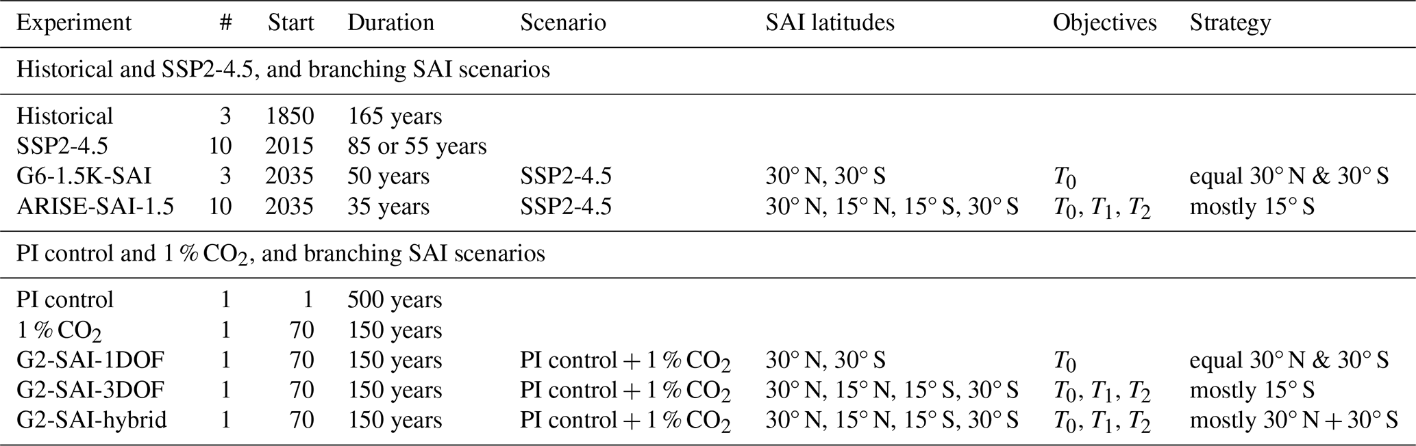
Table 2 Temperature targets for SAI simulations, and the time periods of the respective simulations from which they were derived. Note that, for T₁ and T₂ values, the calculated value can differ by a factor of 3 or 5, respectively, depending whether the scaling factor of $L_{\mathrm{1}}^{\mathrm{2}}$ or $L_{\mathrm{2}}^{\mathrm{2}}$ is included in the denominator of the calculation (compare Lee et al., 2020, Eq. 1, and Kravitz et al., 2017, Eq. 1). Studies have used both definitions; either is correct, as long as one remains internally consistent. We include the scaling factor in our calculations, but include the other value (in parentheses) for completeness.

2.3 Feedback algorithm, temperature targets, and G2-SAI simulation design

As described in the previous section and in Table 1, The G2-SAI-3DOF and G2-SAI-hybrid experiments use the same scenario, set of injection locations, and temperature objectives. However, as we will show in the next section, the injection rates used to meet these targets – and subsequent impacts on the Earth system – are very different. In this section, we explain how injection rates are chosen via algorithm, and why and how the algorithms used for the 3DOF and hybrid experiments are different. This section may not be of interest to the general reader, and those mainly interested in the impacts of different injection strategies on the Earth system may proceed to Sect. 3.

G6-1.5K-SAI and ARISE-SAI-1.5 both use feedforward-feedback proportional-integral control algorithms (colloquially, “feedback algorithms”) to choose injection rates to maintain desired objectives. This approach was first developed to maintain desired T₀, T₁, and T₂ temperature targets with 15 and 30° N/S injections in CESM1 (Kravitz et al., 2016, 2017; MacMartin et al., 2017), and the same framework has since been commonly used in simulation design, as discussed in Sect. 1. The full structure and design of the algorithm is described in the aforementioned studies, but to briefly summarize, the feedback controller consists of constants of proportionality, called gains, which determine how much SO₂ to inject each year. These gains consist of feedforward gains and feedback gains. Feedforward gains prescribe linearly increasing injection amounts based on the expected temperature change (see Fig. 1) and the known sensitivity of temperature to injection in the model, i.e., a “best guess” of how much injection will be needed over time to meet the targets. Feedback gains then adjust the injection rates each year based on the error (the difference between the actual and desired model behavior) over the course of the simulation.

For such a controller, the number of outputs equals the number of inputs, also called the number of degrees of freedom (DOF). In other words, each pair of one feedforward + one feedback gain allows for the control of one climate objective. G6-1.5K-SAI controls for T₀ only (one objective), and therefore requires a “1-DOF” controller with one feedforward gain and one feedback gain. The gains determine the total SO₂ injection rate each year, which is divided evenly between the 30° N and 30° S injection sites. ARISE-SAI-1.5 manages T₀, T₁, and T₂ simultaneously and therefore uses a more complicated “3-DOF” controller with three sets of feedforward and feedback gains, which are named “ℓ₀”, “ℓ₁”, and “ℓ₂” (corresponding to the respective temperature metrics they manage). These gains are handled by the controller in sequence: first, the ℓ₀ gains determine how much SO₂ is placed at 15° N + 15° S to manage T₀; second, the ℓ₁ gains determine whether any of this SO₂ should be diverted to either 30° N + 15° N or 30° S + 15° S to preferentially cool one hemisphere and manage T₁; lastly, the ℓ₂ gains determine whether any 15° N + 15° S injection should be shifted to 30° N + 30° S injection to preferentially cool the high latitudes and manage T₂. The result is some combination of injection across the four latitudes that attempts to meet all three goals simultaneously, but prioritizing T₀ first, T₁ second, and T₂ last. In ARISE-SAI-1.5, this combination largely converges to 15° S injection; this happens because 15° S injection tends to cool the planet relatively evenly in CESM2, but that behavior is model-specific (see Visioni et al., 2023a).

All three G2-SAI simulations also use feedforward-feedback algorithms to choose injection rates: G2-SAI-1DOF uses a 1-DOF algorithm as in G6-1.5K-SAI, and G2-SAI-3DOF uses a 3-DOF algorithm as in ARISE-SAI-1.5. G2-SAI-hybrid also uses a 3-DOF algorithm, but with some changes relative to G2-SAI-3DOF, with the following rationale. T₀ and T₂ changes in the 1 % CO₂ and SSP2-4.5 scenarios are similar for the first 50 years of injection, and the trends continue similarly thereafter for 1 % CO₂ (Fig. 1); however, while T₁ changes are similar initially, T₁ behavior is very different in the two scenarios after the first ∼20 years. T₁ is highly variable in the no-SAI scenarios, likely due to long-term ocean processes in the model. Because of the nonlinear nature of long-term T₁ evolution in the 1 % CO₂ scenario, we use two distinct sets of controller gains in our two simulations with 3-DOF algorithms to more fully explore the design space. In G2-SAI-3DOF, all three pairs of ℓ₀, ℓ₁, and ℓ₂ feedforward and feedback gains are used. In G2-SAI-hybrid, all three feedback gains are used, but the ℓ₁ and ℓ₂ feedforward terms are set to 0. As a result, the 3DOF controller prioritizes 15° S injection, while the hybrid controller “defaults” to 15° N + 15° S injection and has more freedom to adjust the injection strategy as the simulation evolves (this simulation eventually converges to mostly 30° N + 30° S injection, as shown in Fig. 4 below; the term “hybrid” is chosen here to reflect the combined aspects of both the 3DOF and 1DOF strategies).

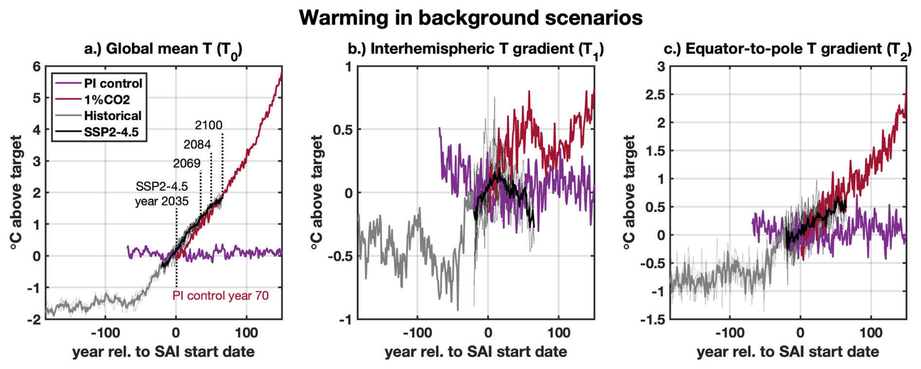
Figure 1 T₀, T₁ and T₂ evolution in the PI control, 1 % CO₂, Historical, and SSP2-4.5 scenarios. The horizontal axis is relative to the year in which SAI scenarios will begin injecting (year 70 of PI control or model year 2035 for SSP2-4.5). The vertical axis is relative to the temperature targets used in the SAI scenarios (PI control 45–95 averages for PI control of 1 % CO₂, and SSP2-4.5 2020–2039 averages for SSP2-4.5; listed in Table 2). For Historical and SSP2-4.5, thin lines represent individual ensemble members, and thick lines represent ensemble means.

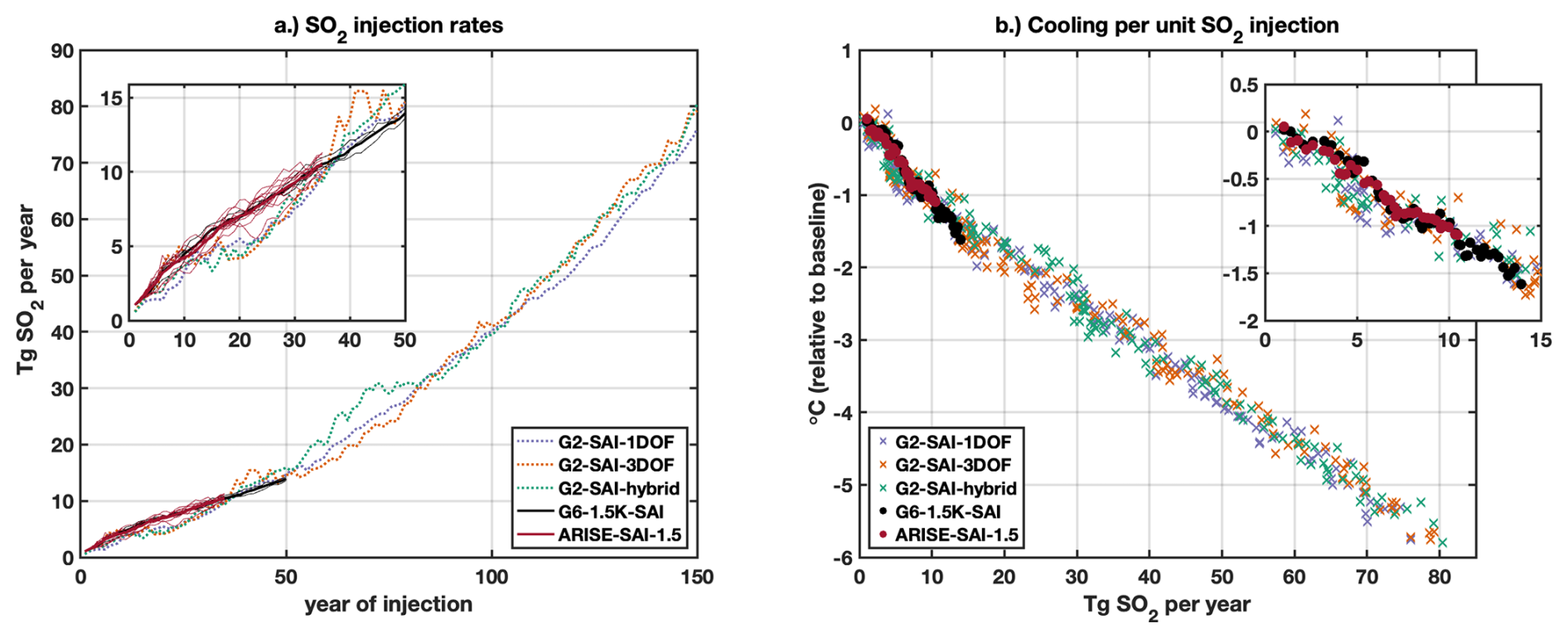
Figure 2 Annual SO₂ injection rates and cooling per unit injection for SAI scenarios. In panel (a), dotted lines are used for G2-SAI and solid lines are used for G6-1.5K-SAI and ARISE-SAI-1.5, with thin lines representing individual ensemble members and thick lines for ensemble means. In panel (b), each marker represents one year of data; x markers are used for G2-SAI, and filled circles are used for G6-1.5K-SAI and ARISE-SAI-1.5 (ensemble means only). In both panels, popout boxes are used to more clearly compare the SSP2-4.5 SAI scenarios with the early period of the G2-SAI scenarios.

3 Results

3.1 G2-SAI SO₂ injection rates, AOD, and temperature response overview

In Fig. 2, we present the total SO₂ injection rates required to maintain the temperature targets (Fig. 2a) and cooling per unit SO₂ injection (Fig. 2b) for the five SAI scenarios. As seen in Fig. 1a, the rates of increase in global mean temperature (T₀) to be offset are similar in the first 50 years of the SSP2-4.5 and 1 % CO₂ scenarios; however, G2-SAI scenarios begin injecting at the same time that temperatures begin increasing (year 70 of PI control, or year 1 of 1 % CO₂) whereas the G6-1.5K-SAI and ARISE-SAI-1.5 scenarios are slightly offset (i.e., begin injecting in 2035 to control to ∼2030 conditions). SO₂ injection rates increase more than linearly for G2-SAI, following the warming trend in the 1 % CO₂ scenario (Fig. 1a). The cooling efficiency per unit injection per year is similar for SAI in the two scenarios for regimes under 10 Tg yr⁻¹ (approximately 1 °C per 10 Tg yr⁻¹ injected); above 10 Tg yr⁻¹, G6-1.5K-SAI cools slightly more efficiently than the average of the G2-SAI scenarios, but this could be variability given the small sample size. For G2-SAI, the injections cool less efficiently above 10 Tg yr⁻¹ (first 50 years, 9.5 Tg yr⁻¹ per 1 °C; years 51-100, 11.6 Tg yr⁻¹ per 1 °C; last 50 years, 13.4 Tg yr⁻¹ per 1 °C). Additional diagnostics concerning injection rates and cooling efficiency are presented in Sect. S1, Table S1 in the Supplement.

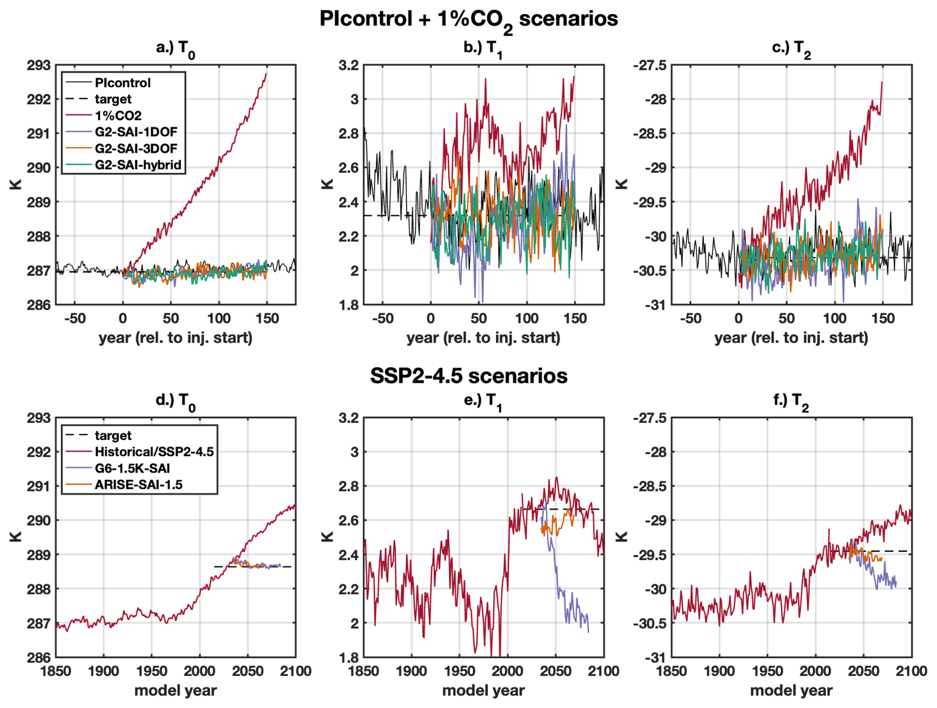
Figure 3 Timeseries of global mean temperature (T₀, left), interhemispheric temperature gradient (T₁, center; positive value indicates warmer NH, negative value indicates warmer SH), and equator-to-pole temperature gradient (T₂, right; more negative value indicates colder poles relative to tropics) for PI control, 1 % CO₂, and G2-SAI scenarios (top) and Historical, SSP2-4.5, G6-1.5K-SAI, and ARISE-SAI-1.5 scenarios (bottom, ensemble means only). Black dashed lines represent temperature targets (PI control 45–95 averages and SSP2-4.5 2020–2039 averages).

In Fig. 3, we present timeseries of T₀, T₁, and T₂ for all SAI and no-SAI scenarios. All 3-DOF SAI scenarios (ARISE-SAI-1.5, G2-SAI-3DOF, and G2-SAI-hybrid) manage T₀ and T₂ well relative to the amount of warming in their respective scenarios, but interannual variability in T₁ is higher relative to long-term change. The hemispherically symmetrical 1-DOF injection strategies (G2-SAI-1DOF and G6-1.5K-SAI) overcool the Northern Hemisphere initially, resulting in negative T₁ and T₂ error (i.e., NH and poles too cold), but G2-SAI-1DOF exhibits both positive T₁ and T₂ error (i.e., NH and poles too warm) by the end of the 150-year simulation.

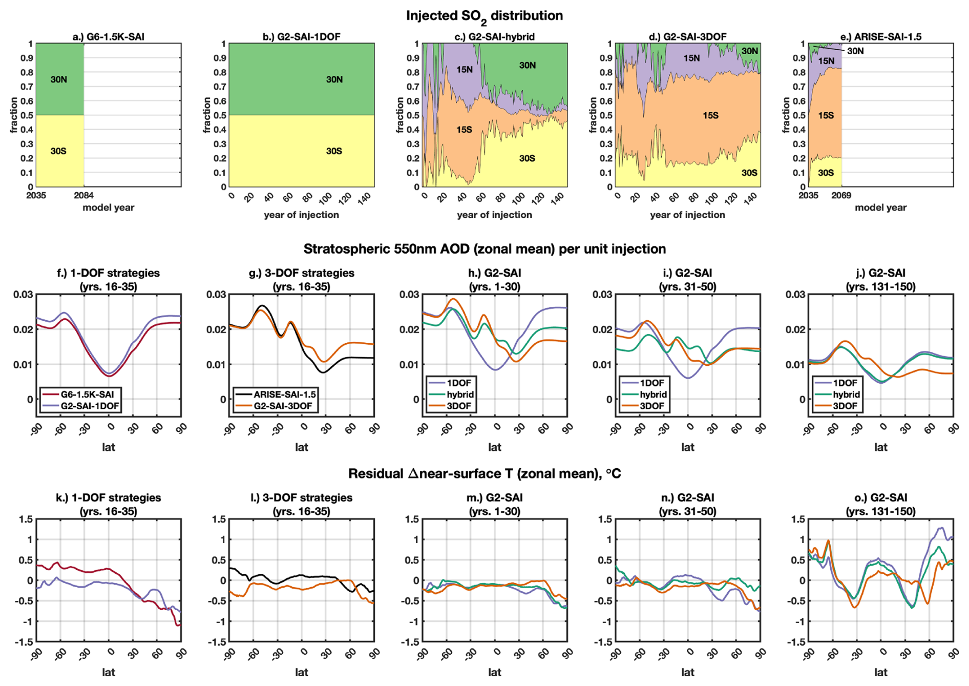
Figure 4 Distribution of SO₂ across latitudes of injection, zonal mean stratospheric 550nm aerosol optical depth (AOD), and zonal mean near-surface air temperature for SAI simulations. For the top row, horizontal axes are scaled to span 150 years to show the relative length of each experiment. In the middle and bottom rows, values in parentheses of panel titles denote years of simulation over which the data are averaged. Temperatures (k–o) are shown relative to the average of the target periods of respective background simulations (years 45–95 of PI control or 2020–2039 of SSP2-4.5). For simulations with multiple ensemble members (ARISE-SAI-1.5 and G6-1.5K-SAI), only ensemble means are shown.

Figure 4 shows differences in how the different SAI simulations meet their respective targets, and the resultant surface temperature distributions. The 1-DOF strategies (G6-1.5K-SAI and G2-SAI-1DOF) inject equal amounts in both hemispheres to control for T₀ only (Fig. 4a–b), with similar distributions of stratospheric 550 nm aerosol optical depth (henceforth “AOD”; Fig. 4f). The three 3-DOF simulations (ARISE-SAI-1.5, G2-SAI-3DOF, G2-SAI-hybrid) distribute injections as needed to maintain T₀, T₁, and T₂ simultaneously to the greatest extent possible. ARISE-SAI-1.5 converges to mostly 15° S injection, supplemented by some 30° S and NH injections (Fig. 4e). G2-SAI-3DOF, designed similarly, converges to a similar distribution, with some long-term variation visible in the extent of 15° N + 15° S versus 30° N + 30° S injection (Fig. 4d); AOD distributions in years 16–35 of injection for G2-SAI-3DOF and ARISE-SAI-1.5 likewise have similar shapes (Fig. 4g). The G2-SAI-hybrid simulation injects less into the SH and more into the NH compared to G2-SAI-3DOF, both initially and in the long-term. This results in slightly less overcooling in the SH and somewhat more initial overcooling in the NH (similar to 1DOF) for G2-SAI-hybrid compared to G2-SAI-3DOF. The larger SH injections in G2-SAI-3DOF may be critical for initiating stronger feedback in the cloud and corresponding warming responses, which required continued larger SH injections in following years. A more detailed investigation of this feedback warrants further study and may have contributed to changes in the AMOC (see below). Over time, the G2-SAI-hybrid injection strategy shifts towards symmetrical injection, and by the end of the experiment, the injection distribution and AOD more closely resemble that of the 1DOF strategy (Fig. 4c, h–j). The 3DOF and hybrid strategies meet the same set of temperature targets, but the zonal mean temperature distributions are different (Fig. 4n–o): the 3DOF strategy has warmer NH subtropics and colder higher latitudes, while the hybrid strategy has colder subtropics and warmer high latitudes.

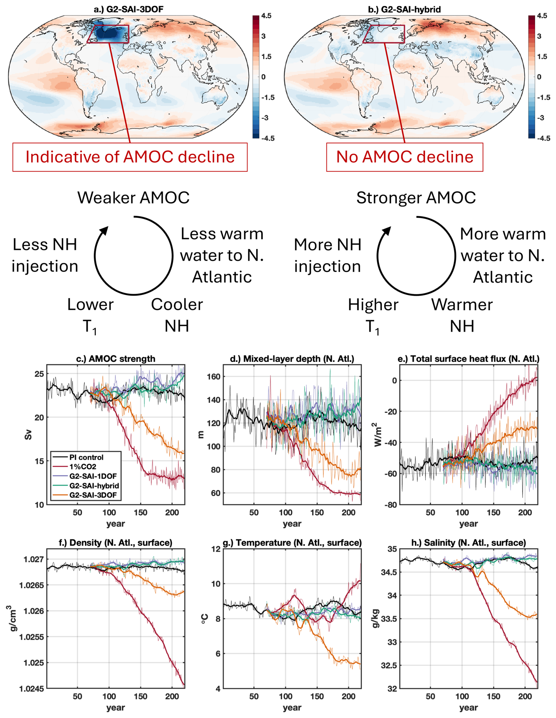
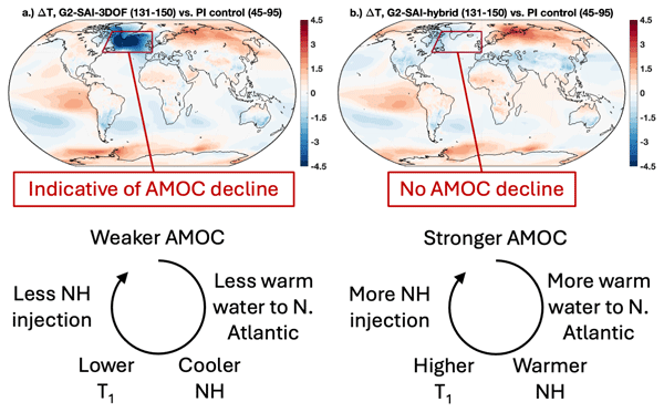
Figure 5 AMOC behavior in G2-SAI runs. Panels (a) and (b) plot changes in near-surface temperature for the last 20 years of G2-SAI-3DOF and G2-SAI-hybrid, respectively, relative to PI control, alongside diagrams explaining how the different injection strategies affect AMOC. The North Atlantic region, defined as the region bounded by the latitudes 45 and 70° N and longitudes 290 and 0° E, is outlined in red. Panels (c)–(h) plot AMOC diagnostics for PI control, 1 % CO₂, and G2-SAI simulations. All diagnostics are shown as thin lines denoting annual means of monthly average data, with thick lines showing 11-year running averages. Panel (c) plots the annual mean strength of the AMOC as computed by the maximum strength of the streamfunction in the Northern Hemisphere. Panels (d)–(h) plot area-weighted output averaged over the North Atlantic, as defined above; panel (d) plots mixed-layer depth; panel (e) plots net surface heat flux; and panels (f), (g), and (h) plot density, temperature, and salinity of the topmost ocean layer, respectively.

3.2 G2-SAI AMOC response

The differences in the NH extra-tropical temperature responses between the G2-SAI-3DOF and G2-SAI-hybrid simulations are partly driven by the corresponding differences in the AMOC response (Fig. 5). The AMOC – Atlantic Meridional Overturning Circulation – is a major feature of the Earth’s circulation: the upper branch carries warm water poleward from the tropics, and the lower branch carries cooler water towards the tropics. Observations and simulations find that the strength of the AMOC is declining under global warming (e.g., Smeed et al., 2018) due to reductions in surface heat fluxes and salinity in the North Atlantic, which reduces the rate of overturning. Studies have found that SAI can mitigate, prevent, or reverse the trend of AMOC decline; Li et al. (2023) attribute the impacts of GLENS and ARISE-SAI-1.5 on AMOC to changes in surface heat fluxes, and Xie et al. (2022) attribute changes to AMOC in G6sulfur to changes in surface ocean-air temperatures, while also finding that freshening from summer sea ice melt may also play a role in its weakening. Bednarz et al. (2025) tested SAI at separate latitudes individually in CESM2(WACCM6), and found that the effect of SAI on AMOC strength was strongly dependent on the latitude of injection; while any of the considered injection latitudes (ranging from 45° N to 45° S) increased AMOC strength relative to the SSP2-4.5 baseline, injections in the Northern Hemisphere had a much stronger impact on AMOC strength and associated predictors, such as North Atlantic sea surface temperatures (SSTs), surface salinity and density.

In agreement with the aforementioned studies, we observe a substantial decrease in the AMOC strength under 1 % CO₂ (Fig. 5c). Such AMOC weakening is consistent with the reduction in the North Atlantic mixed layer depth (Fig. 5d) and surface density (Fig. 5f), driven both by the reductions in the North Atlantic surface heat flux (Fig. 5e; negative values indicate energy loss from the ocean) and salinity (Fig. 5h). Ocean temperatures in the North Atlantic (Fig. 5g) increase initially (∼0–50 years) under global warming but then decrease again as the AMOC weakens and less warm tropical water is transported poleward.

The 3DOF strategy injects largely in the SH throughout the experiment (Fig. 4d). Under this intervention, the decline of the AMOC is slowed down relative to 1 % CO₂ forcing alone, but not prevented entirely; similar trends are seen in mixed layer depth and North Atlantic surface heat flux, density, and salinity, and in the absence of net global warming, North Atlantic ocean temperatures only decrease as AMOC strength declines. Changes in AMOC strength further impact NH surface temperature changes and modulate the SAI injection rates needed to maintain the temperature targets, one of the feedbacks identified by Fasullo and Richter (2023): the weakening AMOC results in a slower transfer of heat from the tropics to the NH mid and high latitudes, decreasing NH vs. SH temperature gradient (T₁) and encouraging more injection in the tropics and SH and less at 30° N (Fig. 5a). In contrast, the 1DOF strategy and hybrid strategies, which inject more in the NH (30° N specifically), maintain the strength of the AMOC (and associated metrics) relative to PI control. The AMOC feedback operates in the opposite direction as under the 3DOF strategy, with the stronger AMOC carrying more heat to the NH mid and high latitudes, increasing T₁ and encouraging more NH injection (Fig. 5b). The result is two SAI strategies which control for the same T₀–T₁–T₂ temperature targets, but result in different temperature distributions which satisfy those targets: G2-SAI-3DOF injects mostly in the SH and maintains the temperature targets with a weak AMOC, warmer NH tropics and subtropics, and cooler NH midlatitudes and pole; and G2-SAI-hybrid injects in the midlatitudes and maintains the same temperature targets in with a strong AMOC, cooler NH tropics and subtropics, and warmer NH midlatitudes and pole (Fig. 4n–o).

While T₁ does not depend solely on AMOC, as other circulation changes that happen as a result of SAI will also affect the distribution of future injections, our results strongly support the conclusions of both Bednarz et al. (2025), in that the injection latitude can have a first order impact on determining the AMOC response to SAI, and Fasullo and Richter (2023), in that the AMOC response itself can further influence the distribution of injection rates needed to reach specific temperature targets. Importantly, and regardless of the cause, our results demonstrate that G2-SAI-3DOF and G2-SAI-hybrid both successfully maintain the same temperature targets by converging to two distinct climate states with different injection strategies. The results thus demonstrate that over longer periods of time, the same T₀–T₁–T₂ combinations can correspond to multiple substantially different climate states. We discuss the implications for SAI experiment design in Sect. 5.

Figure 6 Framework for analyzing the impacts of SAI, using the same nomenclature as Lee et al. (2026). Panel (a) represents a generic hypothetical warming scenario and an SAI scenario in which SAI is used to maintain a constant prescribed temperature, and defines three periods: (1) the “reference period” from which temperature targets are derived; (2) the “warmed world” in which elevated GHG concentrations have increased temperatures relative to the reference period; and (3) the “new climate state” produced by the combination of GHG warming offset by the same amount of SAI cooling. Comparing aspects of the climate across these three periods can help quantify the impacts of global warming (1→2), the impacts of SAI (2→3), and the relative impacts of SAI compared to global warming (1→3). Panel (b) defines these periods for our analysis of the G2-SAI experiments, and panel (c) defines these periods for our analysis of the G6-1.5K-SAI and ARISE-SAI-1.5 experiments.

3.3 Comparison of surface temperature and precipitation responses

In this section, we analyze annual mean temperature and precipitation for the G2-SAI simulations, with select comparisons to the experiments on which they are based (G6-1.5K-SAI and ARISE-SAI-1.5). To do this, we compare maps averaged over selected periods for each experiment: the reference period, the warmed world, and the new climate state reached after offsetting GHG warming with SAI. This is the same framework used by Lee et al. (2026), and the periods for each experiment are defined in Fig. 6. These definitions for periods “1”, “2”, and “3” are used throughout the remainder of the manuscript, as well as in the Supplement.

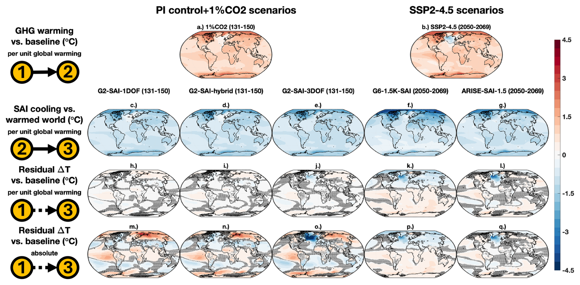
Figure 7 Maps of near-surface air temperature changes for SAI and non-SAI scenarios, across the periods defined in Fig. 6. The top row shows warming in non-SAI scenarios relative to their respective temperature target periods (PI control 45–95 or SSP2-4.5 2020–2039), normalized by the global mean temperature increase since that period (0.91 °C for SSP2-4.5; 5.13 °C for 1 % CO₂). The second row shows cooling in SAI scenarios relative to the same time period in their respective warming scenarios, normalized by the amount of global mean warming. The third and fourth rows plot the temperature difference between SAI scenarios and the respective reference periods to which they control; in the third row, these values are normalized by global warming as in the first two rows, and in the fourth row, these values are not normalized. Shading represents no statistically significant difference between the two samples at the 95 % confidence level according to the two-sample t test.

In Fig. 7, we present maps of temperature changes. In order to compare patterns of warming under GHGs, cooling under SAI, and the combination of this warming and cooling, the three topmost rows are normalized by the amount of warming in the background warming scenario relative to the reference period: 5.13 °C for 1 % CO₂ relative to PI control, and 0.91 °C for late SSP2-4.5 relative to early SSP2-4.5. The first row shows the pattern of the GHG warming at the end of the experimental period (i.e., the last 20 years of injection) relative to the period from which temperature targets are derived, and the second row shows the pattern of cooling due to SAI in the same period. The last two rows plot the residual temperature difference between the last 20 years of SAI and the temperature target period, showing how the imperfect cancellation of the GHG warming and SAI cooling affect regional surface temperatures. Because the lengths of the target periods, amounts of warming, and ensemble sizes are different across the sets of simulations, distributions of the shading denoting statistically insignificant changes are not directly comparable.

Warming patterns across the two background GHG scenarios (Fig. 7a–b) share several broad characteristics, including polar amplification in both hemispheres; increased warming over land relative to the ocean; a “wedge” of increased warming in the Eastern tropical Pacific indicative of an El-Niño-like response; and a warming hole in the North Atlantic indicative of a weakening of the AMOC. All five SAI scenarios also cool the land more than the ocean. This is a common response in SAI modeling experiments; while this has been attributed to the higher heat capacity of water relative to land (Duan et al., 2019), the enhanced warming over land has also been attributed to a number of lapse rate and hydrological feedbacks, which SAI could be preventing (Sutton et al., 2007; Joshi et al., 2008). The relative cooling in the North Atlantic is much stronger in the SSP2-4.5 scenario than in the 1 % CO₂ scenario, as the warming period considered in this study (i.e., the 2020–2039 period to the 2050–2069 period) takes place entirely during the fastest decline of the AMOC, whereas the warming in the 1 % CO₂ scenario averages over the entire AMOC decline, including the plateau at the end (compare Figs. 5c and 9d). The equatorial eastern Pacific warming is visible in the residual temperature maps of all five SAI scenarios, indicating relatively few SAI-induced changes in this mode of climate variability in this model. While absolute temperature residuals are, in general, larger for the G2-SAI scenarios than for the SSP2-4.5-branching SAI scenarios (fourth row), they tend to be smaller per unit of warming being offset (third row). For symmetrical injection strategies, while G6-1.5K-SAI overcools most of the Northern Hemisphere and undercools most of the Southern Hemisphere, G2-SAI-1DOF does not. All three G2-SAI scenarios have substantial residual warming over northern Asia and the Southern Ocean. However, clear differences are visible between G2-SAI-hybrid and G2-SAI-3DOF, showing a substantial cooling over the North Atlantic in G2-SAI-3DOF, which is much weaker for G2-SAI-hybrid, while a slight but significant cooling exists over the continental US, Southern Europe, and Asia, more similar to G2-SAI-1DOF. Determining whether these responses are scenario-specific and/or model-specific will require further study and intermodel comparison; however, the CESM2 simulations of MacMartin et al. (2022) with higher cooling (e.g., the PI +0.5 °C target simulations) do show similar patterns (see Supplement, Sect. S2, Fig. S1), suggesting that this could be a robust response when large injections are used to offset large amounts of warming in CESM2.

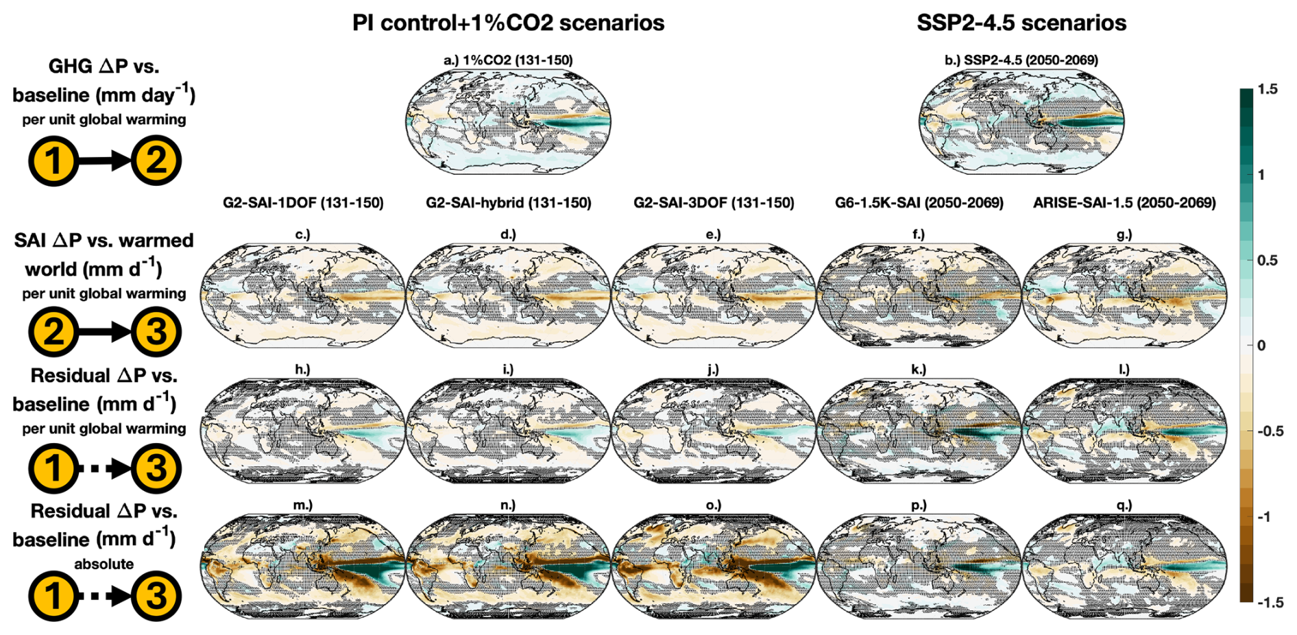
Figure 8 Precipitation, as in Fig. 7 The first, second, and third rows are likewise normalized by degrees of warming in each scenario (0.91 °C for SSP2-4.5; 5.13 °C for 1 % CO₂).

Figure 8 plots precipitation changes. Global mean precipitation is expected to increase under global warming, and it is common result that cooling the planet via the reflection of sunlight decreases precipitation by a greater amount than it increased under GHG forcing; this result has been observed in, among others, the GLENS (Kravitz et al., 2017), ARISE-SAI-1.5 (Richter et al., 2022; Henry et al., 2023), and G6sulfur and G6-1.5K-SAI experiments (Lee et al., 2026). In the PI control baseline period (45–95), global average precipitation is 2.91±0.01 mm d⁻¹ (± denoting the standard deviation of annual means); by the last 20 years of 1 % CO₂, it has increased to 3.14±0.02 mm d⁻¹, while under G2-SAI, it instead decreases to 2.76±0.02 mm d⁻¹ (1DOF), 2.72±0.02 mm d⁻¹ (3DOF), and 2.75±0.02 mm d⁻¹ (hybrid), offsetting approximately 175 % of the increase under global warming. In comparison, ARISE-SAI-1.5 and G6-1.5K-SAI offset 119 % and 106 %, respectively, of the precipitation increase under SSP2-4.5 between the 2020–2039 and 2050–2069 periods. More study is needed to understand whether this pattern is robust across models, or CESM specific. Detailed investigation of regional and seasonal rainfall changes is beyond the scope of this paper. Additionally, the G2-SAI simulations have only one ensemble member each, and due to the high variability of precipitation, analyses of specific impacts would benefit from multiple ensemble members.

Both warming scenarios result in southward shifts and net increases in tropical precipitation; increased precipitation in the midlatitudes and polar regions in both hemispheres; and smaller changes in many parts of the subtropics, though not everywhere. All five SAI interventions reduce precipitation in the midlatitudes and poles in both hemispheres and in the tropics, but the cancelation of the GHG effect is largely imperfect, with residual drying or wetting in one or both hemispheres and a chevron-shaped pattern of residual wetting and drying in the tropical Pacific. G2-SAI-3DOF and ARISE-SAI-1.5 both show increased drying over land in the tropics relative to the 1-DOF strategies. G2-SAI-3DOF also has stronger residual drying in the North Atlantic and southwest Europe. Plots comparing zonal mean precipitation among the simulations considered in this study are provided in the Supplement (Sect. S3, Fig. S2).

4 ARISE-SAI-1.5, revisited

Using the knowledge gained from our G2-SAI simulations, we revisit the ARISE-SAI-1.5 experiment. ARISE-SAI-1.5 was designed to balance policy-relevant and science-relevant objectives, with the strategy and timeline chosen to simulate a plausible, globally coordinated deployment of SAI to stabilize global temperatures in the near future. Since its publication, the ARISE-SAI-1.5 datasets have been used to investigate several potential impacts of SAI, including on the cryosphere in the Arctic (Lee et al., 2023) and Antarctic (Goddard et al., 2023), agriculture (Grant et al., 2025), monsoon (Sagar and Chakraborty, 2025), extreme weather (Touma et al., 2023), and many others.

ARISE-SAI-1.5 uses the same feedforward-feedback control algorithm to choose injection rates as the G2-SAI experiments; the algorithm has evolved very little since its introduction by MacMartin et al. (2017). During the controller design process for that experiment (and this one), it was assumed that the Earth system response to SAI was sufficiently linear such that, in the absence of variability and uncertainty, there existed one combination of injection rates to produce a desired temperature response; the feedforward is the best estimate of that combination, and the feedback corrects for the presence of variability and uncertainty. However, as we have shown above, small changes to the controller parameters can result in diverging system responses, which ultimately reach the same large scale near surface temperature targets despite very different injection rates and more distinct regional changes. As such, had the design process proceeded differently, the injection rates and impacts of ARISE-SAI-1.5 could have looked very different. While the initial ARISE-SAI-1.5 experiment only runs for 35 years, there would be no practical reason why SAI should end abruptly in 2070 (especially considering the risks of a termination shock), since global warming and required injection rates would still be increasing after that time, a real-world deployment of SAI could plausibly continue for much longer. Hence, the long-term implications of the injection rate choices used for ARISE-SAI-1.5 are worth considering.

We do not claim that the specifications or performance of the controller used in ARISE-SAI-1.5 were flawed or deficient, or that the injection rates used were in any way “wrong”. Rather, knowing that there may exist multiple unique combinations of injections across the same set of latitudes that can maintain the same T₀–T₁–T₂ distribution, we attempt to modify the original control algorithm to determine whether we can find another solution that meets the same temperature targets, but potentially results in fewer or different side effects. Specifically, we modify the feedforward to encourage the controller to transfer as much injection as possible from 15° N and 15° S to 30° N and 30° S, similarly to the differences between G2-SAI-3DOF and G2-SAI-hybrid. We accomplish this by using the same controller as the original, but prescribing an additional ℓ₂ feedforward gain equal to the ℓ₀ gain; because ℓ₀ determines the amount of 15° N + 15° S injection, and ℓ₂ determines the amount of this which is changed into 30° N +  30° S injection, this has the effect of converting all 15° N + 15° S injection into 30° N + 30° S until the feedback portion of the controller decides otherwise. In other words, instead of “starting” with 15° N + 15° S injection and moving some of it to 30° N and/or 30° S as the controller determines, we now start with 30° N + 30° S and transfer to 15°  as needed.

We run three ensemble members of this new configuration, “ARISE-hybrid” (named after G2-SAI-hybrid), using the same model configuration and settings as the original ARISE-SAI-1.5 ensemble as described in Richter et al. (2022) and branching from the same initial conditions as ensemble members 001, 002, and 003. The experiment is successful (see Supplement, Sect. S4, Fig. S3 for T₀, T₁, and T₂ timeseries): as shown in Fig. 9, the original controller places around 60 % of the injected SO₂ at 15° S and around 20 % each at 15° N and 30° S; our modified controller meets the same targets by placing about 40 % at 15° S, about 35 % at 30° S, and 25 % at 30° N. The injection rates for the new controller are slightly higher overall, as the controller needs more Tg of SO₂ to manage global mean temperature with 30° N/S injection than with 15° N/S injection.

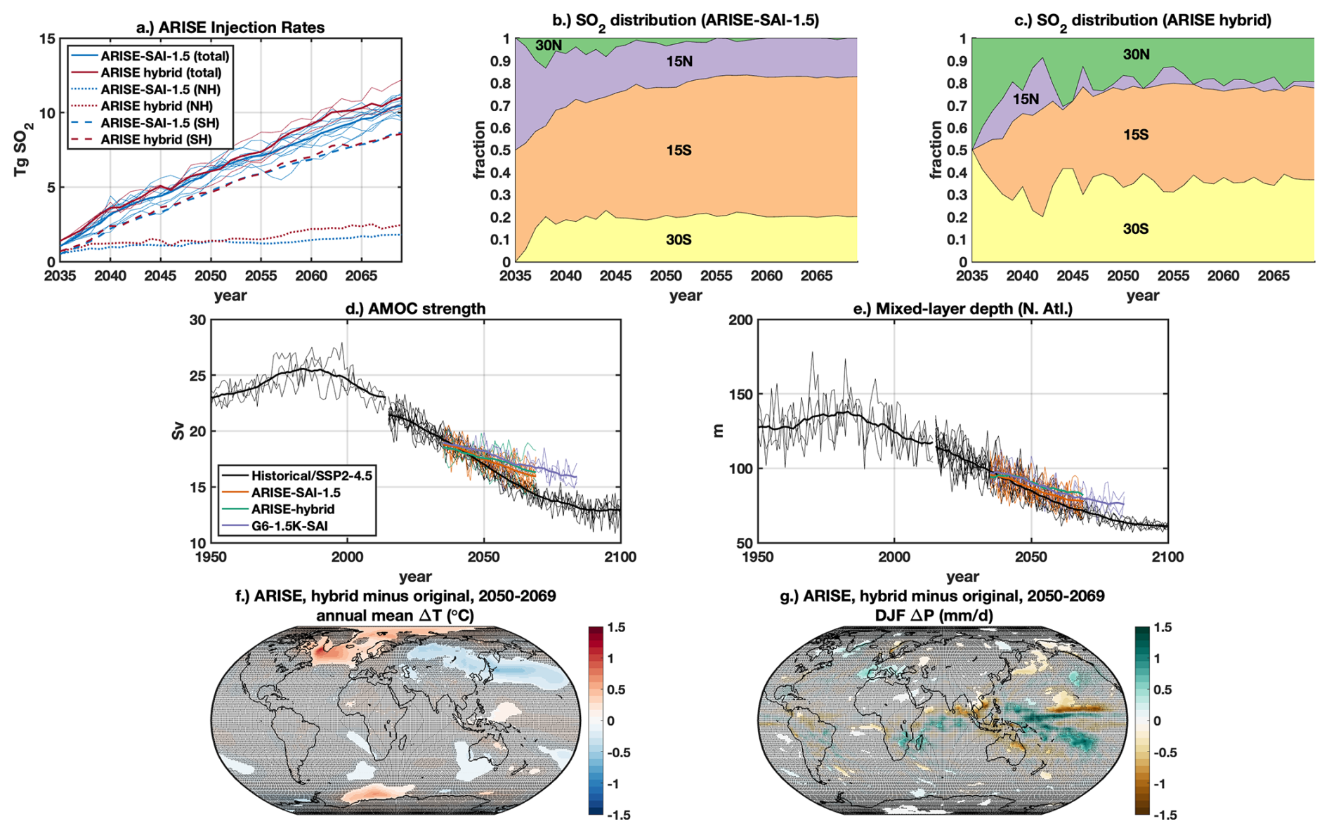
Figure 9 Comparison of original ARISE-SAI-1.5 simulations and new ARISE-hybrid simulations with a modified controller. Panel (a) shows total SO₂ injection rates (solid lines), as well as total NH and SH injection rates (dotted and dashed lines, respectively); thin lines (total injection only) denote individual ensemble members, and thick lines denote ensemble means. Panels (b) and (c) show the partition of these injections across individual injection latitudes for original and new simulations, respectively. The middle row plots AMOC strength (d) and North Atlantic mixed-layer depth (e), as in Fig. 5, for Historical, SSP2-4.5, and SSP2-4.5-branching SAI scenarios; thin lines plot individual ensemble members, and thick lines denote 11-year running averages of ensemble means. The bottom rows plot differences in annual mean near-surface air temperature (f) and winter (DJF) precipitation (g) between ARISE-hybrid and ARISE-SAI-1.5, averaged over the last 20 years of simulation (2050–2069); shading denotes areas with no statistically significant difference at the 95 % confidence level according to the two-sample t test.

By shifting a greater fraction of the injected SO₂ from 15° S to 30° N, we would expect the intervention to have a stronger restorative effect on the strength of the AMOC, as well as a relative shift of the ITCZ towards the Southern Hemisphere (while T₁ is often used as a proxy for ITCZ position, the two are not perfectly linked, and the ITCZ could change without changing T₁, or vice versa – see Lee et al., 2020). On average, the AMOC strength (Fig. 9d) and North Atlantic mixed layer depth (Fig. 9e) under ARISE-hybrid is higher than under ARISE-SAI-1.5. While the signal-to-noise ratio of these metrics is very low over the short experiment duration, AMOC strength in both of these ARISE experiments is also slightly lower than in G6-1.5K-SAI, which is consistent with expectations, but mixed layer depth in ARISE-hybrid is slightly higher than in G6-1.5K-SAI, which is contrary to expectations, Nonetheless, surface temperature differences in the North Atlantic and North Pole for ARISE-hybrid relative to ARISE-SAI-1.5 (Fig. 9f) are statistically significant and consistent with a stronger AMOC; we also see increased winter precipitation in that region (Fig. 9g). In addition to these responses, we see a southward shift of tropical precipitation, which is statistically significant in some areas. Other aspects of the response are less easily explained; the increased cooling in the subtropics and midlatitudes over Asia and the Pacific, and the increased cooling over parts of the SH midlatitudes, could be directly explained by the increased injections at 30° N and 30° S, respectively, but may also be indicative of circulation changes (Bednarz et al., 2023).

We do not argue here that our new ARISE injection strategy is “better” than the original, or vice versa; rather, the key result here is that a second solution to the control problem exists, and that Earth system responses to the two solutions may be different in significant ways. Changes in AMOC are subtle, suggesting that a reversal of its slowdown may not be feasible with modest, short-term SAI. We reserve a deeper analysis of the differences for a future study, but at first glance, there are statistically significant differences in the pattern of the short-term surface response, and there may be longer-term implications as well: the increase in 30° N injection could affect long-term AMOC behavior, and the additional injection at 30° S may have implications for the stability of the ice shelves in the Antarctic (Goddard et al., 2023). Shifting the injection rates away from the tropics (i.e. 15° S) to subtropics (30° N + S) will also have implications for the magnitude of SAI-induced stratospheric heating and the associated changes in circulation, which may be responsible for some of the surface temperature changes discussed above (Bednarz et al., 2023).

5 Conclusions

In this study, we propose G2-SAI as a GeoMIP experiment and present three new 150-year SAI simulations that model contemporary injection strategies against a PI control background with 1 % CO₂ forcing. Assessing SAI responses in such an idealized set-up, excluding transient changes driven by forcings other than CO₂, is expected to more robustly reveal commonalities and differences in the fundamental responses to SAI among different ESMs. In particular, here we demonstrated that slightly modifying feedback controller settings can have a significant impact on surface climate through AMOC responses. While we have demonstrated this in one model, it is not clear if other models respond similarly. In addition to serving as comparison points for their future-scenario counterparts, ARISE-SAI-1.5 and G6-1.5K-SAI, our G2-SAI simulations demonstrate that, in the long term, two SAI strategies which control for the same temperature-based objectives can meet those targets in different ways: our G2-SAI-3DOF simulation maintains a set of T₀–T₁–T₂ temperature targets with mostly 15° S injection and a weak AMOC state, while our G2-SAI-hybrid simulation maintains the same targets with mostly 30° N and 30° S injection and a strong AMOC state.

Our experiments demonstrate a limitation of the T₀–T₁–T₂ controller framework. During the controller design process of MacMartin et al. (2017) and Kravitz et al. (2017), the relationship between injection rates, AOD, and temperature change is approximated as linear and therefore perfectly additive. These studies do acknowledge the existence of nonlinearities in these relationships; however, any SAI simulation that computes controller gains by scaling the original gains (a process which is not well documented, but is usually a similar process to that described by Sect. 2 of Lee et al., 2025) will compute exactly one solution to the control problem. As we have shown, the implicit design choices made during the controller-building process can be more impactful than previously thought. Moving forward, we recommend a more complete description of controller implementation in future experiments, including not only the targets but also their respective priorities, injection strategies used to reach each one, and the authors' motivations for their choices.

Using this information, we revisit the ARISE-SAI-1.5 experiment and design a revised injection strategy that meets the same temperature targets as the original while shifting as much as possible of the injection to 30° N and 30° S. Comparing hybrid and 3DOF ARISE and G2-SAI experiments, the distribution of SO₂ across injection latitudes is moving towards the NH, but the difference is not as stark in ARISE as the difference between the G2-SAI 3DOF and hybrid simulations. There are statistically significant differences in the surface response, but while some differences in the AMOC response were found, these are not as pronounced for ARISE as for G2-SAI. Since the ARISE experiment is by the design much shorter, it cannot be said whether or not the two sets of ARISE simulations would eventually diverge in such a pronounced way as the G2SAI runs if extended for much longer (i.e., one with a strong AMOC, and one with a weak AMOC). However, the purpose of the ARISE-hybrid experiment is not to produce an ARISE-like simulation that recovers the AMOC, but rather, to demonstrate the extent to which the injection strategy can change while still meeting the same injection targets. This is significant for two reasons: firstly, ARISE-SAI-1.5 was designed to be a highly policy-relevant scenario, and represents a plausible example of a future SAI intervention to limit the impacts of global warming while also minimizing side-effects and residual warming to the greatest extent possible given current levels of understanding and the complexity of the system. Our results show that, even within the restrictions of one set of T₀–T₁–T₂ temperature targets and the same four injection latitudes, there is not “one way” to implement SAI, and the span of possible outcomes can be significant, even after only 35 years. Secondly, the ARISE-SAI-1.5 dataset has undergone substantial analysis on the perceived impacts of a policy-relevant SAI scenario since its publication. Had the controller design process gone differently, the impacts of the 10-member ensemble could have been perceived differently, and we recommend that this be taken into account when future experiments are designed.