Global relevance of atmospheric and land surface drivers for hot temperature extremes

Hot temperature extremes have severe impacts on society and ecosystems. These extremes are driven by both atmospheric and land surface processes, such as advection or reduced evaporative cooling. The contributions of the individual drivers to the formation and evolution of hot extremes have been analyzed in case studies for major past events, but the global relevance of drivers still remains unclear. In this study, we determine the relevance of (i) atmospheric drivers, such as wind, geopotential height, horizontal geopotential height differences, and surface net radiation, and (ii) land surface drivers, such as evaporative fraction and enhanced vegetation index, for hot extremes across the globe using observation-based data. Hot extremes are identified at daily and weekly timescales through the highest absolute temperature, and the relevance of the considered drivers is determined with an analogue-based approach. Thereby, temperature anomalies are analyzed from situations with driver values similar to those of the hot extreme. The results show that geopotential height at 500 hPa is overall the most relevant driver of hot extremes across the globe at both timescales. Surface net radiation and evaporative fraction are the second most relevant drivers in many regions at the daily timescale, while wind is the second most relevant at the weekly timescale. Regional variations in the relevance of individual drivers are largely explained by different climate regimes. Revealing key regions and influential timescales of land surface drivers on hot extremes can inform more efficient prediction and management of the increasing threat these extremes pose.

1 Introduction

Hot extremes are severe weather events characterized by prolonged periods of excessively high temperatures. These events pose significant risks to human health, agriculture, ecosystems, and infrastructure, making the understanding of their drivers a critical area of research (Anderegg et al., 2013; Goulart et al., 2021; Anderson and Bell, 2011; McEvoy et al., 2012). Moreover, because of the increasing trend in global temperatures, hot extremes have become longer, more frequent, and more intense in recent years (Seneviratne et al., 2023).

Hot extremes are often found to be linked to the atmospheric circulation anomalies. For example, studies by Woollings et al. (2018) and Brunner et al. (2017) highlight the importance of blocking systems and jet stream anomalies for the onset and development of these events, especially in mid-latitudes. These quasi-stationary high-pressure systems disturb the westerly flow for several days to weeks, leading to prolonged extreme surface temperatures (Brunner et al., 2017; Kautz et al., 2022). For instance, Wehrli et al. (2019) demonstrate the importance of atmospheric circulation as a key driver that trapped warm air masses and exacerbated surface heating during the 2010 Russian heatwave. Similarly, persistent atmospheric pressure patterns were one of the key drivers of the 2003 European heatwave (Miralles et al., 2014).

On the other hand, land surface feedback mechanisms, including evaporative cooling deficits and vegetation water stress due to low soil moisture, can exacerbate the hot extremes and lead to multi-hazard events (Wulff and Domeisen, 2019; Teuling et al., 2010; Miralles et al., 2014; Hauser et al., 2016). Similarly, a study by Benson and Dirmeyer (2021) identified a critical “soil moisture breakpoint”, below which the probability of heatwaves increases due to a shift in surface energy fluxes from latent to sensible heat. This sensitivity becomes even more pronounced as soil moisture approaches the “permanent wilting point”, where vegetation can no longer draw water from the soil, leading to a substantial increase in local surface temperatures. As a result, the sensitivity to soil moisture deficits significantly contributes to the severity of heat events (Dirmeyer et al., 2021). This effect underscores the spatial variability in soil moisture–temperature feedback mechanisms across different climatic zones. Specifically, transitional regions, where latent heat flux strongly depends on soil moisture, exhibit more pronounced land–atmosphere coupling (Wehrli et al., 2019; Koster et al., 2004).

However, a joint and comparative assessment of these drivers is lacking, such that the relative importance of the land surface compared to that of atmospheric drivers is unclear (Perkins, 2015). Moreover, the drivers and underlying processes leading to hot extremes have mostly been studied in regional case studies to identify the drivers of specific events (Wehrli et al., 2019; Fischer et al., 2007). Hence, a global analysis to complement and reconcile the existing regional studies is missing (Sillmann et al., 2017), and there is no single commonly accepted definition of hot extremes such that previous research has employed different temperature metrics or related indices and at different timescales (Perkins and Alexander, 2013; Brunner et al., 2017; Raha and Ghosh, 2020). All this limits our understanding regarding the physical mechanisms leading to hot extremes across the globe and our skill to forecast these events.

We aim to address these knowledge gaps here by conducting a global analysis where we determine and compare the relevance of atmospheric and land surface drivers of hot extremes. This includes the identification of relevant spatial patterns and regions of particular interest for each considered driver variable. In this context, we define hot extremes through the highest absolute temperatures and consider daily and weekly timescales. Focusing on different timescales allows us to reveal to which extent the drivers of hot extremes, and the spatial patterns of their relevance, change with different event durations. For this purpose, we employ an analogue approach to identify physical mechanisms leading to hot extremes. In particular, we focus on two distinct types of analogues. (i) We use flow analogues, which have been widely studied in the literature (Jézéquel et al., 2018; Yiou et al., 2014, 2007) and are based on atmospheric circulation patterns that closely resemble the flow conditions of selected hot extremes. (ii) As a novel aspect of our work, we introduce land surface analogues, which are derived from land surface conditions, such as vegetation states and energy balance at the surface, which are similar to the respective conditions in a selected hot extreme. By integrating land analogues into our analysis, we aim to explore how land surface processes contribute to the development and persistence of heatwaves, offering a complementary perspective to the traditional focus on atmospheric dynamics. Consequently, this can yield insights into potential differences between the mechanisms underlying the formation of hot extremes across timescales and regions.

2 Data and methods

2.1 Considered drivers of hot extremes

The considered land surface and atmospheric drivers of hot extremes in this study are selected based on the existence of plausible physical pathways through which they can affect near-surface temperature (Table 1). Atmospheric variables include wind speed and geopotential height at three different atmospheric pressure levels which influence the distribution and movement of heat within the atmosphere (Xoplaki et al., 2003). Specifically, we analyze geopotential height and wind at three atmospheric levels: surface, 850 hPa, and 500 hPa. The selection of these three levels is based on their relevance to the formation and evolution of hot extremes and on findings from the existing literature (Jézéquel et al., 2018). The surface level can provide information about the advection of warm air (Jiménez-Esteve and Domeisen, 2022). The 850 hPa level, situated approximately 1.5 km above sea level, is used to assess lower-tropospheric processes. The 500 hPa level, roughly 5.5 km above sea level, is often related to the formation of hot extremes due to blocking mechanisms at this level (Zschenderlein et al., 2019). This level is important for capturing mid-tropospheric patterns and the influence of large-scale atmospheric circulation on weather systems (Ventura et al., 2023). In addition, we use horizontal geopotential height differences at 500 hPa as a proxy for the geostrophic wind.

Table 1 Summary of considered driver variables.

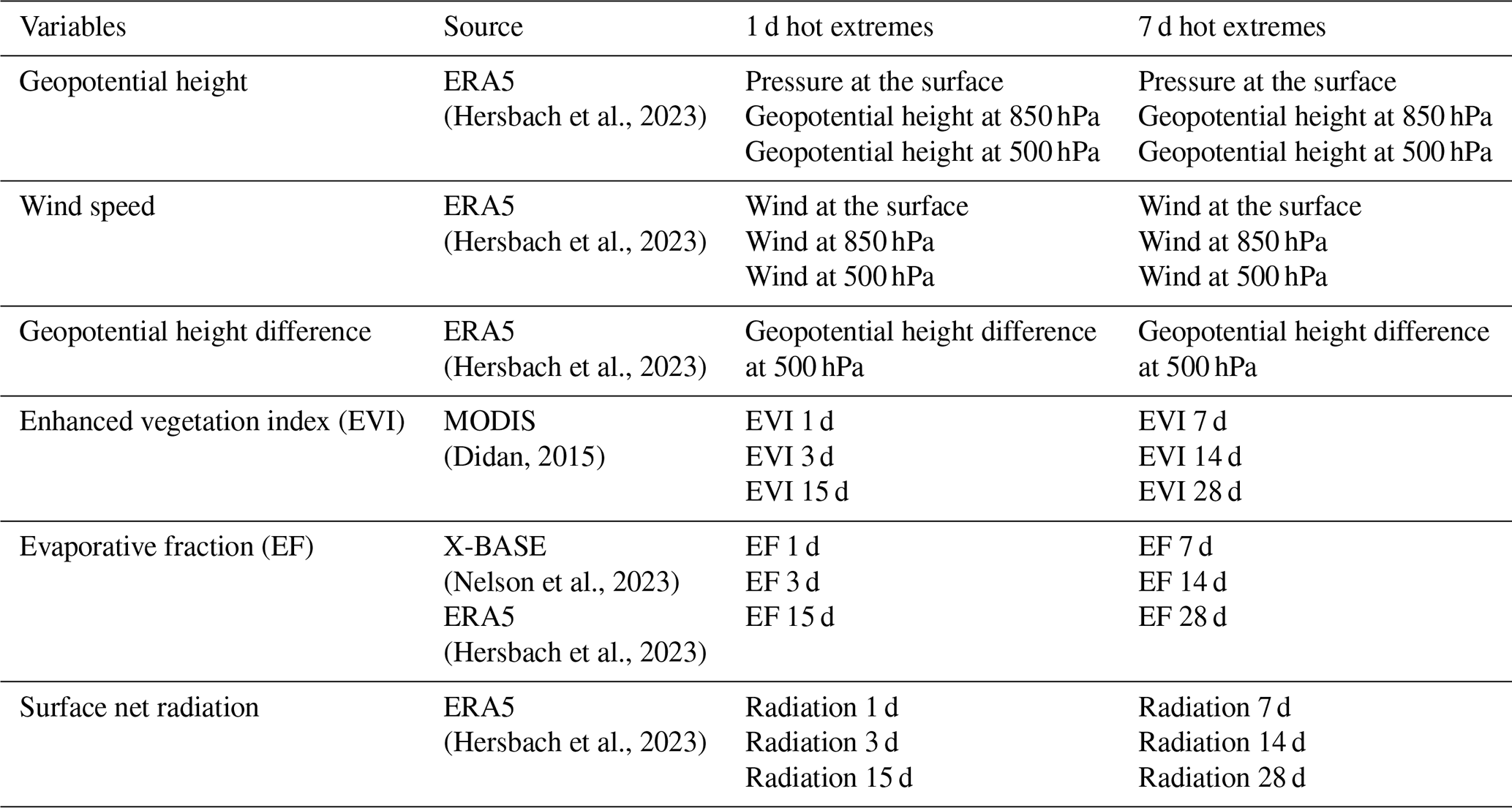
Land surface variables, such as evaporative fraction (EF), enhanced vegetation index (EVI), and surface net radiation, impact near-surface temperatures through the provision of energy and evaporative cooling, as well as albedo, which determines the amount of reflected solar energy (Seneviratne et al., 2010). We analyze the land surface variables across the same timescales considered for the hot extremes but also at longer timescales, in order to capture potential lagged effects arising from an accumulation of the influence of land surface variables over time, given their relatively slower variability compared to the atmospheric drivers. These timescales are important for understanding plant responses to hot extremes: water loss and stomatal closure are more pronounced on the daily timescale, while, on the daily to weekly timescale, vegetation is affected by leaf wilting and senescence (Zhang et al., 2016).

We consider two different timescales to define hot extremes, 1 d and 7 d. This allows us to test to which extent the underlying drivers depend on the considered timescale. The spatial and temporal resolutions considered are 0.25° and daily intervals, respectively, for the study period from 2001–2020. This period was selected because the evapotranspiration data from the X-BASE dataset used to calculate EF are only available during these years. EF is computed by normalizing evapotranspiration by surface net radiation. Notably, this calculation incorporates variables from two different datasets: X-BASE and ERA5. This approach is justified, as X-BASE is formulated using ERA5 data. In cases where the native resolutions of the datasets differed from the ones mentioned, the datasets were aggregated to a spatial resolution of 0.25° and a daily temporal resolution using linear interpolation. Regarding the limited global coverage of the EF dataset, we mask grid cells without data, such as Greenland, in all considered datasets to ensure consistency in spatial coverage. In addition, we compute the horizontal geopotential height differences at 500 hPa pressure level for each grid cell with respect to the values in adjacent grid cells in the northern, eastern, southern, and western directions.

To capture potential lagged effects arising from an accumulation of the influence of land surface variables over time, we average land surface variables at different time windows depending on the hot extreme timescales considered. For example, for 1 d hot extreme events (Table 1, third column), we use values on the day of the event, an average of the variables on the event day and the 2 preceding days, and an average of the variables on the event day and the 14 preceding days. Similarly, for 7 d hot extremes, we consider time windows of 7, 14, and 28 d to compute the average of the land surface variables.

2.2 Definition of hot extreme events

For our definition of hot extremes, we use the 2 m daily mean temperature, as this accounts for both daytime and nighttime conditions. We make this choice because nighttime temperatures are relevant for impacts of hot extremes on human health, they play a role in the physiological response of plants to hot extremes (Wahid et al., 2007), and this way we can also capture trends in nighttime extreme temperatures (Wu et al., 2023). These daily means used in our analysis are computed based on UTC instead of local time. While this choice may lead to phase mismatches in diurnal cycles for some variables, particularly in regions where local time differs significantly from UTC, it provides consistency across datasets, which is essential for our analysis.

We identify the hot extreme events in each grid cell based on the highest absolute temperature values within our study period from 2001–2020. The selected events occur during the warm seasons, as we pick the events with the highest temperatures.

For the 1 d hot extreme events, we select three individual days with the next-highest temperatures, ensuring that each selected day is at least 15 d apart from the others to maintain independence, as shown in Fig. 1a. Likewise, for the 7 d timescale, we select the three 7 d periods with the next-highest average temperatures, also ensuring that they are at least 15 d apart from each other for independence. In order to further illustrate the event selection of 1 d hot extremes within the study period (2001–2020), let us assume in a specific grid cell that the hottest day recorded during this period is 15 July 2012. After selecting this day, we mask out 15 July and the 30 d surrounding it (1–30 July) to prevent the selection of any overlapping or consecutive days in the further selection process. We then identify the second-hottest day from the remaining days of the time series after the masking, which could be 5 August 2010, and apply the same 15 d masking around this date (21 July–20 August). This process is repeated to find the third-hottest day, ensuring that all 3 selected days are at least 15 d apart, maintaining their independence.

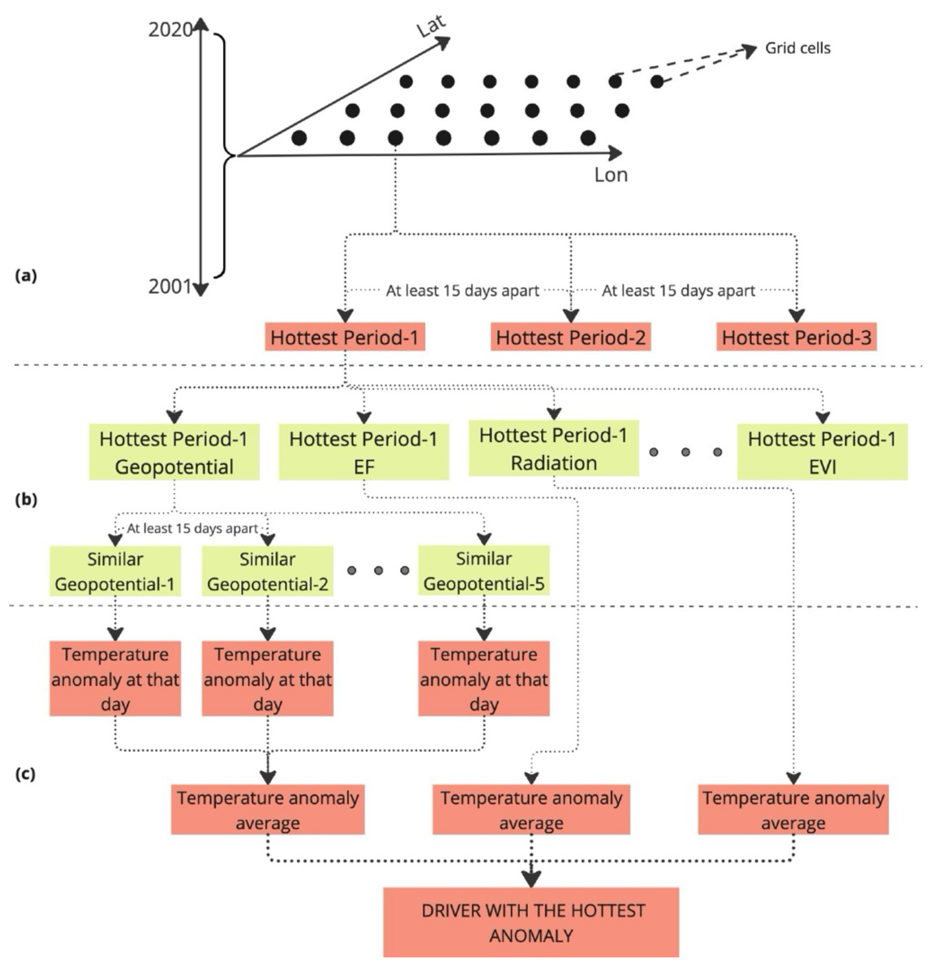
Figure 1 Workflow for determining main drivers of hot temperature extremes. Hottest periods refer to 1 or 7 d hot extreme events. See text for details. This figure was created using miro.com.

For 7 d hot extreme events, the procedure is similar. Suppose the highest 7 d average temperature in the grid cell occurs from 10–16 July 2015. We mask out this period and the surrounding 30 d (26 June–1 August) to select the next-highest 7 d period, such as 20–26 August 2013. This ensures that each selected 7 d event is independent.

2.3 Description of the analogue approach

After identifying hot extremes, we determine the values of the considered driver variables for each event, and, based on them, we identify analogues as illustrated in Fig. 1b. For each driver and at each considered atmospheric level (in the case of geopotential height and wind) and temporal scale (in the case of EVI, EF, and surface net radiation), we select the five periods in which the driver variable values are most similar to those observed during the identified hot extremes. This approach shares a conceptual basis with the analogue methods in the literature, such as those used by Jézéquel et al. (2018) and Yiou et al. (2007). These studies show that selecting more than five geopotential height analogues has little effect on the results.  To maintain consistency, we use the same number of five analogues for each driver variable. The analogue analysis is done separately for each grid cell; i.e., analogues always come from the same grid cell as where the hot extreme was detected. These analogues are only selected at a similar time of year to the original hot extreme event to ensure comparable conditions; this is needed because, for example, circulation patterns with westerly winds from the North Atlantic tend to cool Europe in summer while warming it in winter or because EVI or EF anomalies are only comparable across a similar phase of the growing season. For this purpose, a 120 d window surrounding the specific calendar date (i.e., month and day) of the relevant hot extreme event is considered across all years to select the analogue periods. These selected periods are also at least 15 d apart from each other to ensure independence.

We note that the “closeness” of the selected analogues to the observed values on the day/week of the event can influence our results. In general, the analogues resemble the extremes well (Fig. A1). They tend to be closer to the observed values for the 1 d extremes than the analogues for the 7 d extremes. Analogues for radiation in the high northern latitudes are most different from the extremes, with an underestimation of the observed radiation of 20 % or more locally. This makes it less likely to detect radiation as a main driver in these regions.

2.4 Degree of relevance index

For each driver, we compute a degree of relevance which describes the fraction of the observed temperature anomaly of the selected hot extremes, which is detected in the related analogues for each driver variable, as shown in Fig. 1c.

For each variable D (e.g., geopotential height, EVI, EF), we identify 15 analogue periods based on similarity to the three hottest observed extremes (5 analogues each) in each grid cell. The degree of relevance for each variable D in each grid cell “g” is computed as Eq. (1):

$$\begin{array}{}\text{(1)}& \text{degree of relevance of}D\left(g\right)={\displaystyle \frac{\mathrm{1}}{\mathrm{15}}}{\sum }_{i=\mathrm{1}}^{\mathrm{15}}\left({\displaystyle \frac{T_{\text{analog}}^{\prime }(g,i)}{{\stackrel{\mathrm{‾}}{T}}_{\text{event}}^{\prime }\left(g\right)}}\right).\end{array}$$

$T_{\text{analog}}^{\prime }(g,i)$ denotes the temperature anomaly (climatological mean temperature subtracted from the temperature values recorded) during the ith analogue period in grid cell g, based on the conditions of driver D. ${\stackrel{\mathrm{‾}}{T}}_{\text{event}}^{\prime }\left(g\right)$ is the mean temperature anomaly calculated from the three observed hottest extreme events in the grid cell g. It serves as a basis of comparison to determine how much of the observed extreme temperature anomaly can be explained by the analogue temperature conditions of variable D. This indicates the fraction of the actual temperature anomaly that can be explained with one driver, i.e., the degree of relevance of the dominant driver in the considered hot extreme events. The expected degree of relevance ranges between 0 and 1. Values close to 1 indicate that hot extremes are explained to a great extent by the considered variable. The dominant driver in a grid cell is then selected as the variable with the highest degree of relevance. It is important to note that this approach assumes a linear and separate contribution of each driver, which is a limitation when interactions between drivers are relevant. We note that, with our approach, the cumulative degree of relevance from different drivers can exceed 1 due to collinearities among the Earth system variables. However, as we explain in more detail in Sect. 3.2, this is typically not the case.

2.5 Analysis of driver independence

In our methodology (Sects. 2.3 and 2.4), we assume that atmospheric and land surface variables are independent as drivers of hot extremes. In order to assess the extent of their independence, we compute cross-correlations among the driver variables across several regions worldwide. This avoids relationships canceling out between different regions. We focus on 5×5 grid cell (1.25°×1.25°) clusters among regions with different climatic and land surface characteristics (i.e., central Europe, the Amazon rainforest, Australia, central Asia, southern Africa, and North America). To avoid potential biases from a single cluster per region, we select three separate 5×5 subregions, thus capturing a broader spectrum of climatic and topographic conditions (Fig. A2). Within each subregion's 25 grid cells, we have three hot extreme events per grid cell (as mentioned in Sect. 2.2). This results in $\mathrm{5}\times \mathrm{5}\times \mathrm{3}=\mathrm{75}$ observations per subregion for calculating the correlations between variables. By averaging the correlation results across the three subregions for each region ($\mathrm{75}\times \mathrm{3}=\mathrm{225}$ observations), we obtain an aggregated indicator of the correlation of variables.

2.6 Attribution analysis

In order to analyze the spatial distribution of the dominant driver variables identified for 1 and 7 d hot extremes with respect to different land surface characteristics and climatic regimes, we employ a random forest approach (Breiman, 2001; Molnar, 2022). Therein, the spatial patterns of the degree of relevance of geopotential height and EF serve as target variables, while aridity, tree cover, irrigation, silt soil fraction, 2 m temperature, total precipitation, surface net radiation, soil moisture, and topography are used as predictors (Fig. A3). We split the data into training and testing sets, with 25 % of the data reserved for testing. We used 100 trees and a maximum depth of 10 to configure the RandomForestRegressor, as these hyperparameters have been proved to work well in other studies (Oshiro et al., 2012; Probst and Boulesteix 2017). Bootstrapping was enabled, and the feature importance was evaluated using mean absolute SHapley Additive exPlanations (SHAP) values (Lundberg and Lee, 2017; Sundararajan and Najmi, 2019) to provide insight into the contribution of each predictor.

2.7 Effect of the positive trend in hot temperature extremes on the relevance of driver variables

In light of the increasing trends in global temperature extremes (Seneviratne et al., 2023), we analyze potential changes in the relevance of the considered drivers of hot extremes over time. For this purpose, we divide the study period into two periods, 2001–2010 and 2011–2020, and employ the same methodology as described in Sects. 2.1–2.4 to calculate the relevance of all driver variables for each of the time periods. We also determine the significance of the changes in relevance through bootstrapping. For this purpose, we use the original 15 analogues (3 hot extremes × 5 analogues per hot extremes = 15 analogues) per grid cell and per time period (2001–2010 and 2011–2020) and draw a random sample of 15 from them (with replacement). Resampling is done 1000 times. Then, we compare the mean degrees of relevance of the resampled 15 analogues from both periods per grid cell such that we can infer significance from analyzing whether a substantial fraction (e.g., 950 out of the 1000) of the mean degrees of relevance between the two time periods is consistently above or below zero.

3 Results and discussion

3.1 Global distribution of most relevant driver variables

The global distribution of the dominant driver variables for hot extremes on both 1 and 7 d timescales is illustrated in Fig. 2. A more detailed depiction of drivers' relevances across pressure levels and timescales is presented in Fig. A4. The results are aggregated across geopotential height levels in the case of atmospheric variables and across timescales in the case of land surface variables. The map corresponding to the 1 d timescale reveals that geopotential height is the predominant driver, accounting for approximately 60 % of the analyzed area. More specifically, the 500 hPa level geopotential height is most influential in mid-latitude regions. This finding supports the existing literature that highlights the significant role of atmospheric blocking mechanisms in the formation of hot extremes in these latitudes and at 500 hPa pressure level (Pfahl and Wernli, 2012; Brunner et al., 2017; Jiménez-Esteve and Domeisen, 2022). Conversely, in primarily tropical regions, surface net radiation substantially influences the occurrence of 1 d extreme temperature events. This can be understood as lateral temperature and pressure gradients being weaker in the tropics such that atmospheric circulation is less relevant, while, instead, solar radiation is intense because of a larger and near-direct solar incident angle. Next to this, EF is found to be the most relevant driver of hot extremes across 10 % of the study area. This is particularly the case in central North America and central Asia, which are known as transition regions between wet and dry climate. In these regions, evapotranspiration and consequently evaporative cooling are relatively high but also limited by soil water availability, which is typically low during hot extremes (Koster, 2004; Wang et al., 2007). This way, reduced soil moisture and, as a result, lower-than-usual EF lead to higher sensible heat flux, resulting in increased surface temperatures during hot extremes (Schwingshackl et al., 2017; Teng et al., 2016). Similarly, the findings of Röthlisberger and Papritz (2023) show that diabatic heating is a factor affecting the temperature anomalies, especially in regions where the soil moisture is limited.

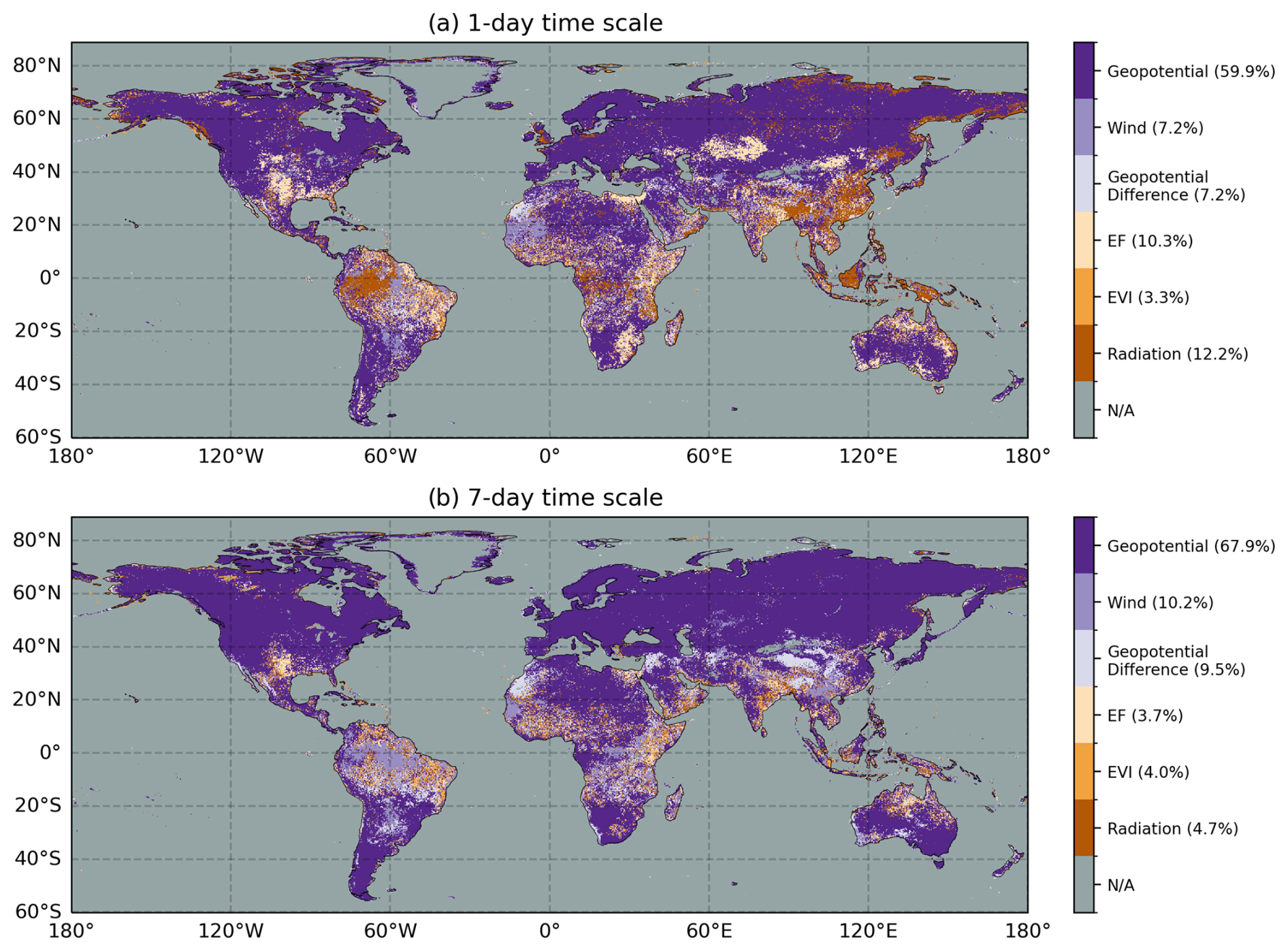
Figure 2 Dominant driver variables identified for 1 and 7 d hot extremes. The percentages indicated on the color bar reflect the proportion of the study area where hot extremes are most influenced by each variable.

For drivers of hot extremes at the 7 d timescale, we find that geopotential height remains the most dominant variable globally for 7 d hot extremes, while its relative influence increases with respect to the 1 d hot extremes in mid-latitudes. This can be related to the formation of blocking systems during which a stationary high-pressure system blocks the westerly flow at mid-latitudes (Brunner et al., 2017), causing clear-sky radiative forcing, subsidence of air masses, and air warming (McGregor, 2024). In the case of the land-surface-related variables, EVI in particular affects hot temperatures through shading in tropical or semi-arid warm regions. In the identified regions where EVI is most relevant through the vegetation response to incoming solar radiation and emission of longwave radiation (McPherson, 2007), temperatures can reach levels at which leaves start to wilt, which then reduces shading-related cooling and further amplifies the temperatures (Brun et al., 2020). This indicates that heat can accumulate through higher-than-usual radiation persisting over some time (Miralles et al., 2014). Furthermore, land surface variables affect hot extremes mostly at the same timescale of the hot extremes, while lagged effects are of minor relevance (Fig. A4 and Table A1).

The main driving variables of hot extremes are summarized in Fig. 3 with respect to climate regime, as classified through long-term means of temperature and aridity (calculated as the ratio of long-term mean surface net radiation and long-term mean daily accumulated precipitation). The choice of temperature and aridity in this context is justified by an additional analysis in Sect. 3.2 and Fig. A3. Geopotential height is the most relevant driver across both cold and warm regions and dry and wet climate regimes for both 1 and 7 d timescales. At the 1 d timescale, in warm regions, radiation is the second most relevant driver and is related to more intense solar radiation in low to medium latitudes. The land surface variable EF is the second most important driver in dry climate regimes. This is related to the fact that water availability is just about sufficient for vegetation in these regions, which means that (i) it can supply significant evaporative cooling, while, (ii) during warm and dry conditions, water availability will not be sufficient such that evaporative cooling decreases, which in turn contributes to enhanced temperatures. For the 7 d timescale, wind becomes relevant for warm regions next to geopotential, which probably relates to the advection of warm air from remote regions (Domeisen et al., 2022; Zschenderlein et al., 2019), while radiation and EF are less relevant.

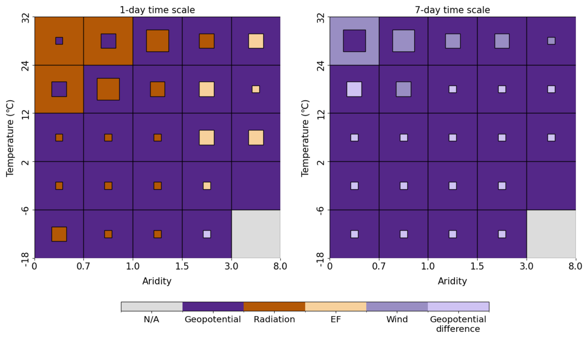
Figure 3 Main driving variables of hot extremes summarized across climate classes. The colors of the boxes indicate which driver is most influential in the largest number of grid cells within the climate class. The color of the inner square indicates the second most relevant driver. The size of the square denotes the relative relevance of the second most important driver: large squares are used if the number of grid cells where the second most relevant driver is most influential exceeds 65 % of the number of grid cells where the most relevant driver is most influential. Likewise, medium-sized squares are used for fractions of 25 %–65 %, and small squares are used for fractions of<25 %. Note that, if there are fewer than 20 grid cells to represent the corresponding variables, the boxes will appear in gray or any other single color. The latter is the case when there are sufficient grid cells of the most dominant variable but an insufficient number of grid cells for the second most dominant variable. The number of grid cells in each category is shown in Fig. A5.

These results have to be seen in the context of some limitations. The analogue methodology employed here does not account for interactions between the considered driver variables. This means that temperature anomalies associated with the analogues of a given variable could also partly result from anomalies in another variable that is closely connected to the first one and will hence add to its effect. We expect that the consideration of several hot extremes and of multiple analogues for each extreme can mitigate this problem as different weather and vegetation conditions characterize each of them. Furthermore, our main goal is to disentangle land surface and atmospheric drivers of hot extremes which are not expected to be strongly related to each other. This assumption is tested by performing a cross-correlation analysis of the variables for each selected region (see Sect. 2.5). Overall, we find that most correlations are below 0.5 (=25 % of shared variance), with some exceptions. While some moderate correlations exist within atmospheric variables or land surface variables, correlation of land and atmospheric variables is low for most considered regions (Fig. A6).

Another limitation is the data quality of each driver variable. A lower signal-to-noise ratio for certain variables compared to others may affect the identification of analogues and related temperature anomalies and consequently the estimated relevance of the variable. However, we observe consistent spatial patterns across different datasets, which lend credibility to our results and align with the existing literature on land surface and atmospheric drivers for hot extremes (Jimenez-Esteve and Domeisen, 2022). At the same time, we use established products which are all comprehensively validated; hence we expect that differences in data quality between individual data streams do not have an effect on our results.

3.2 Relative roles of the most important atmospheric and land surface drivers

In this section, we analyze the main land surface and atmospheric drivers in more detail in terms of their degree of relevance. The latter is calculated as the fraction of temperature anomalies of hot extremes explained by each driver according to the temperature anomalies of their analogues. Figure 4 presents the results for EF and the geopotential height for 1 and 7 d hot extremes. The relevance of EF diminishes from daily to weekly timescales, suggesting that vegetation influences on extreme heat primarily operate over short durations with immediate effect. This is likely because, at longer timescales, the evaporative cooling effect becomes less dominant as atmospheric advection transports air masses from other regions, overshadowing local land–atmosphere interactions. Conversely, the relevance of geopotential height increases from daily to weekly timescales, especially in the mid-latitudes, coinciding with the regions where Pfahl and Wernli (2012) found that atmospheric circulation was highly related to extreme summer temperatures. This can be related to the persistence of the blocking systems for several days to weeks (Brunner et al., 2017), exacerbating the subsidence of air masses and air warming for longer time periods (McGregor, 2024).

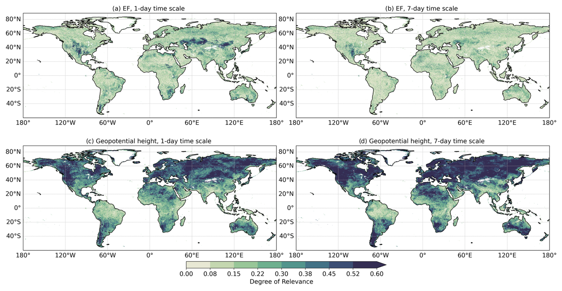
Figure 4 Degree of relevance of EF (a, b) and geopotential height (c, d) at daily and weekly timescales. The degree of relevance is computed as the ratio between the respective analogue temperature anomalies and the observed temperature anomalies during hot extremes.

In the next step, we determine the drivers of the spatial patterns of the relevance of geopotential height and of EF in supporting hot extremes. This is done with a random forest analysis (Sect. 2.6). We find that long-term mean temperature and radiation are the most relevant predictor variables for both 1 and 7 d hot extremes (Fig. A3). Additionally, aridity and topography (based on the standard deviation of subgrid altitude values) play an important role for both timescales of hot extreme events, while the other considered variables are less important.

In the following, we group the global results with respect to long-term averages of temperature and aridity; temperature is chosen, as it is found to be the most relevant variable, and aridity is chosen instead of radiation because it covers another aspect of climate (e.g., including water input to the land surface), while radiation is more linked with temperature. Accordingly, we summarize the results from the global degree of relevance of EF and geopotential height in different climatic regions (Fig. A7). Although EF is the second most dominant variable (after geopotential height) in semi-arid and arid regions as shown in Fig. 3, it has a relatively higher degree of relevance in those regions compared to wet regions. On the other hand, geopotential height is more relevant in colder climates. These findings highlight that climate is the main modulator of the relevance of drivers of hot extremes across regions.

Furthermore, we study potential changes in the relevance of the considered drivers of hot extremes between the periods 2001–2010 and 2011–2020 (Fig. A8). We find only small changes. While these could be related to natural decadal variability, we find that radiation and EVI are becoming slightly more relevant at both considered timescales, which may also be related to global greening (Zhu et al., 2016; Chen et al., 2019) and global brightening (Wild, 2009). At the same time, the changes are significant only in relatively small fractions (<10 % for most drivers) of the study area.

Moreover, we calculate the sum of the degree of relevance of the three most influential variables at each grid cell (Fig. A9). This indicates which fraction of the observed hot temperature anomalies can be explained with our approach. The maps show that a large part of the observed hot temperature anomalies can be explained within the analogue approach. This suggests that we have considered relevant and meaningful driver variables. The explained fractions of hot extreme temperature anomalies are slightly lower in some tropical and subtropical regions. This can be related to lower quality of land surface datasets due to sparse observations and partly dense vegetation cover and to the influence of sea surface temperatures on hot extremes in these regions (Orth and Seneviratne, 2017). Note that the consideration of sea surface temperatures or other remote forcings on hot extremes is outside the scope of this study. Correspondingly, we also do not focus on timescales longer than 7 d. Note further that in this calculation we do not jointly consider variables which are related to each other, i.e., geopotential height and geopotential height difference or EVI and EF, such that we mitigate the effect of collinearities among the considered drivers. If such related variables are among the three most influential variables, we consider instead the next most relevant variable which is less related to the variables already considered. In some cases, the cumulative degree of relevance of the variables could exceed a value of 1 due to collinearities among driver variables. Typically, however, this is not the case, as shown in Figs. 4 and A9. This indicates that dependencies between driver variables are not critically affecting our analysis.

4 Conclusions

This study provides a global analysis of the potential drivers of hot extremes, considering a selection of atmospheric and land surface variables. The results highlight that geopotential height, particularly at the 500 hPa level, is globally the dominant driver for hot extremes, especially in mid-latitude regions. This finding underscores the important role of atmospheric circulation anomalies, such as atmospheric blocking, in the formation of hot extremes (Pfahl and Wernli, 2012). In contrast, surface net radiation is more influential in tropical regions, where it is more intense and constant throughout the year and can therefore exacerbate hot conditions at any time. Land surface variables, like evaporative fraction and enhanced vegetation index, influence hot extremes in transitional regions (semi-arid to arid), which are neither wet nor dry, such that they can sustain significant evapotranspiration. Moreover, evapotranspiration depends on water availability such that soil moisture (i.e., a land surface variable) variability influences evapotranspiration and consequently the surface energy balance and temperature (Denissen et al., 2024; Seneviratne et al., 2010).

These results complement the existing literature on drivers of hot extremes by jointly considering and comparing the relevance of atmospheric versus land surface drivers, which have so far been largely studied in isolation. Another novel aspect in our study is the consideration of hot extremes at different timescales. As the timescale of hot extremes is not clearly defined in the literature, we focus on daily and weekly timescales in order to analyze potential differences of drivers' relevances across timescales. By examining both 1 and 7 d timescales, we capture different phases of heatwaves: 1 d events reflect the peak of extreme heat, while 7 d events represent persisting hot conditions. This approach allows us to infer that atmospheric drivers are slightly more relevant at longer timescales, whereas land surface drivers, such as surface drying and reduced evaporative cooling, are slightly more relevant at shorter timescales. This may be related to the fact that local evaporative cooling is overshadowed by the advection of air from other regions via the large-scale circulation at longer timescales. Another interesting result of our study is that, despite the increase in hot extremes in response to global warming, there is no clear global shift in the relevance of the drivers. We find only regionally significant changes in the relevance of geopotential height, EVI, and radiation. It remains unclear, however, if the small changes in drivers' relevances during a relatively short 20-year study period can be interpreted as an indication of negligible changes in the mechanisms underlying hot extremes in future decades up until the end of the century.

Our findings imply that weather forecasting models and Earth system models need to be able account for various mechanisms leading to hot extremes in order to yield accurate forecasts of unfolding hot extremes and future projections of their occurrence and intensity. In particular, inclusion of vegetation phenology could be crucial, as variables like EVI and EF are linked to vegetation processes, such as canopy conductance and stomatal resistance, which play a significant role in driving hot extremes. However, many current forecasting models do not sufficiently exploit the available vegetation data such that they use only mean seasonal cycles instead of near-real time dynamics, for example (Ruiz-Vásquez et al., 2023; Duveiller et al., 2022). Including these processes would improve the representation of land–atmosphere interactions, which is vital for enhancing the accuracy of hot extreme predictions. This way, our study motivates (i) further efforts to model the vegetation response to hydro-meteorological conditions at high spatial resolution, where the coupling between vegetation and weather can be most accurately represented, and (ii) interest to monitor the root zone soil moisture dynamics to better constrain vertical and lateral soil water movement in land surface models such that they can yield more accurate estimates of plant-available water.

Previous research has shown in a case study that hot extremes cause most impacts in terms of societal attention and public health at timescales between 2 weeks and 2 months (De Polt et al., 2023). This highlights the need for more comprehensive and multidisciplinary studies that build on our findings to investigate and compare the relevance of different drivers of hot extremes at weekly to monthly timescales. Such studies could integrate atmospheric, land surface, and oceanic influences to provide a holistic understanding of the mechanisms behind prolonged hot extremes. Considering the role of ocean variability and broader spatial patterns, including teleconnections, could help reveal how large-scale climatic factors interact with local conditions to intensify or sustain extreme heat events. This broader perspective could be useful for enhancing predictive models and informing adaptive strategies in the face of increasing climate variability.

Appendix A

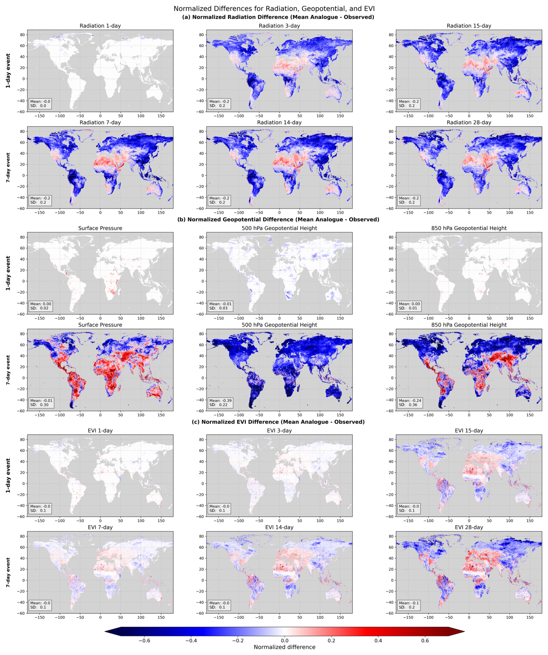
Figure A1 Spatial patterns of normalized differences of geopotential height, radiation, and EVI between the mean values of the five analogue periods and the values of the observed hot event divided by the local 20-year standard deviation. Note that this figure shows the average differences across the three hottest periods. Mean and standard deviation values are denoted in the bottom-left corner of each map.

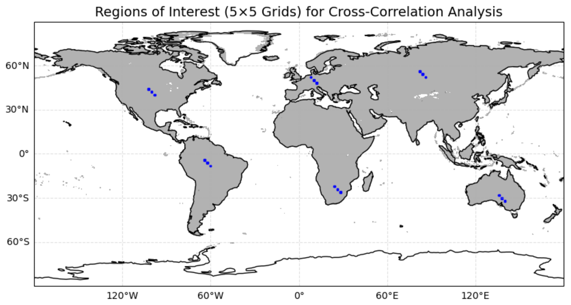
Figure A2 Selected regions from central Europe, the Amazon rainforest, Australia, central Asia, southern Africa, and North America. Each region is divided into three subregions, and, within each subregion, a 5×5 grid cell cluster is used to assess the cross-correlation of driver variables during hot extreme events.

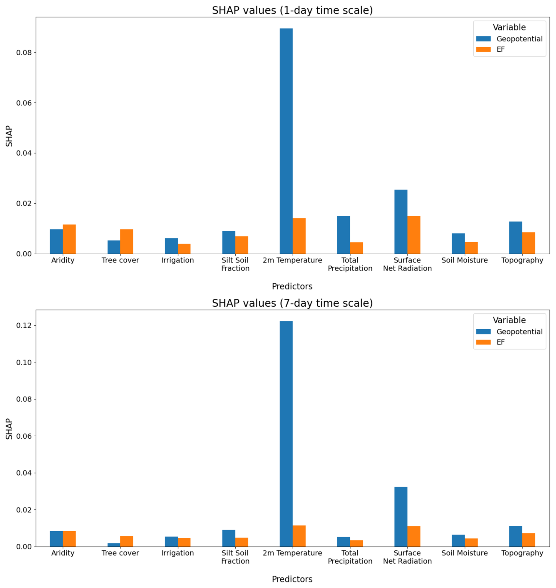
Figure A3 Relative importance (SHapley Additive exPlanations (SHAP) values) of multiple factors to explain the spatial patterns of geopotential height and EF as the main drivers for 1 and 7 d hot extremes.

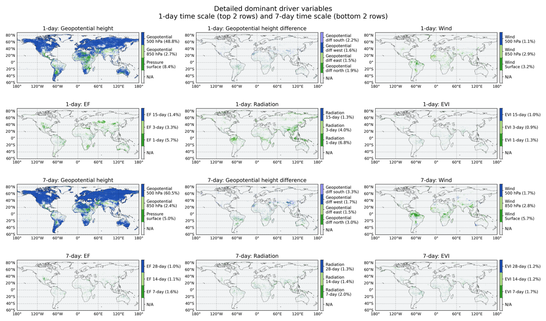
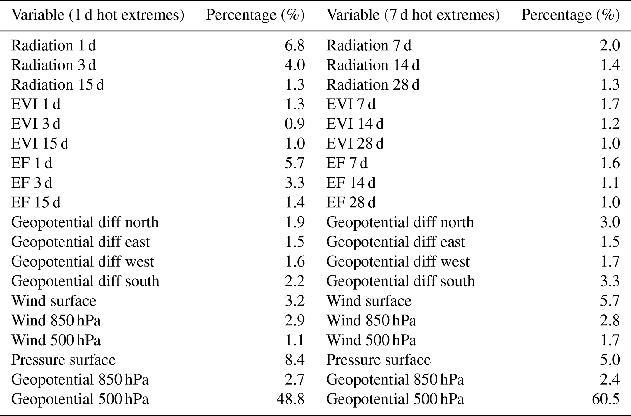
Figure A4 Detailed dominant driver variables identified for 1 d (top two rows) and 7 d (bottom two rows) timescales are shown for six variable groups: geopotential height, geopotential height difference, wind speed, EF, radiation, and EVI. Each colored grid cell indicates the dominant variable within the respective group. Gray grid cells (N/A) indicate areas where the dominant driver either belongs to a different variable group than the one currently plotted or has missing data. Percentages provided in parentheses next to each color bar indicate the area-weighted fraction of the total analyzed area where each variable is identified as the dominant driver. These percentages represent the area over which each variable is dominant when considering all variables collectively within each timescale separately. These results are summarized in Table A1.

Figure A5 Total number of grid cells in each temperature–aridity category.

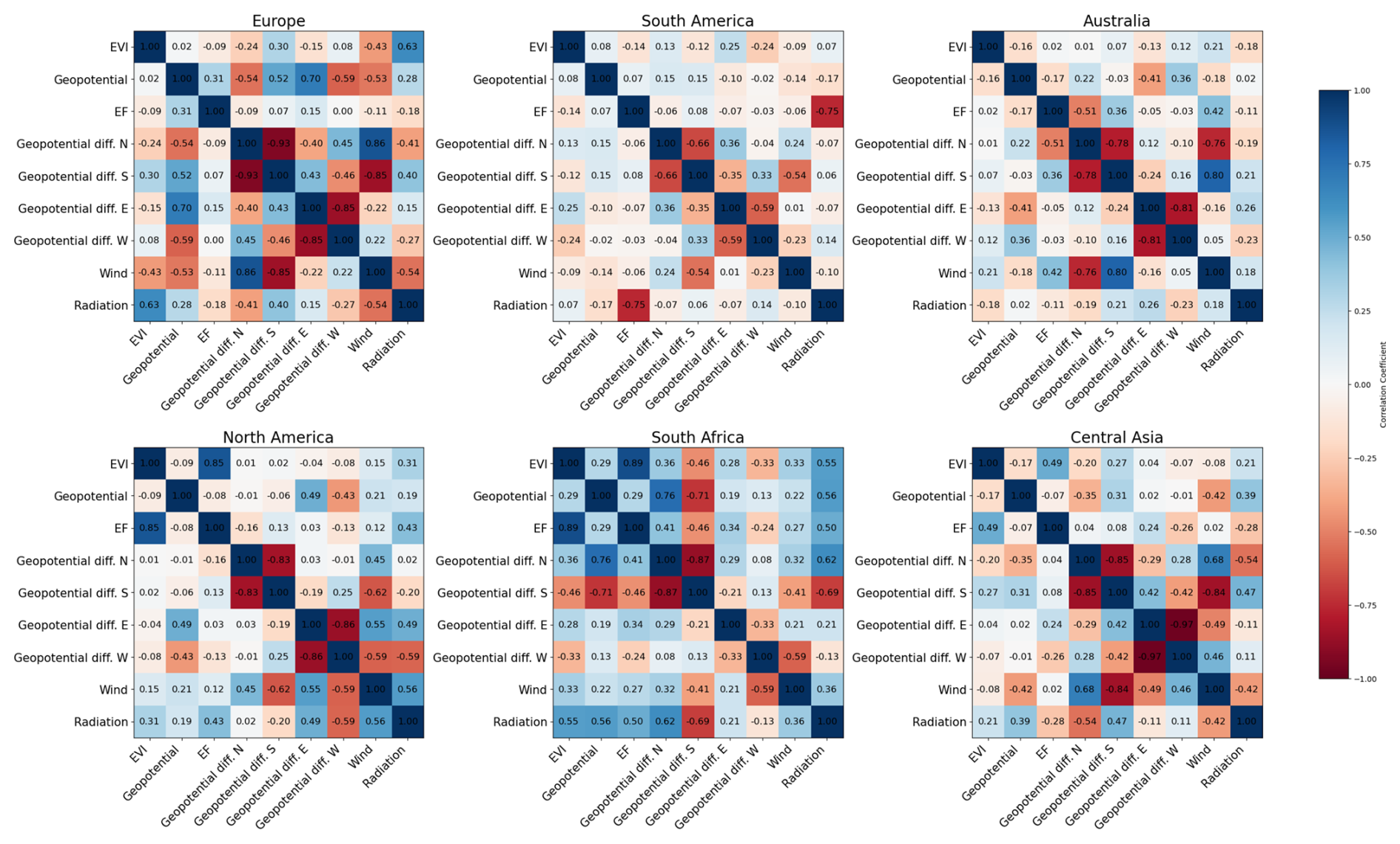
Figure A6 Spearman cross-correlation matrix for the six land surface (EVI, EF, radiation) and atmospheric (geopotential height, wind, geopotential height difference (north, south, east, west)) variables, averaged across three subregions within each region (see Sect. 2.5).

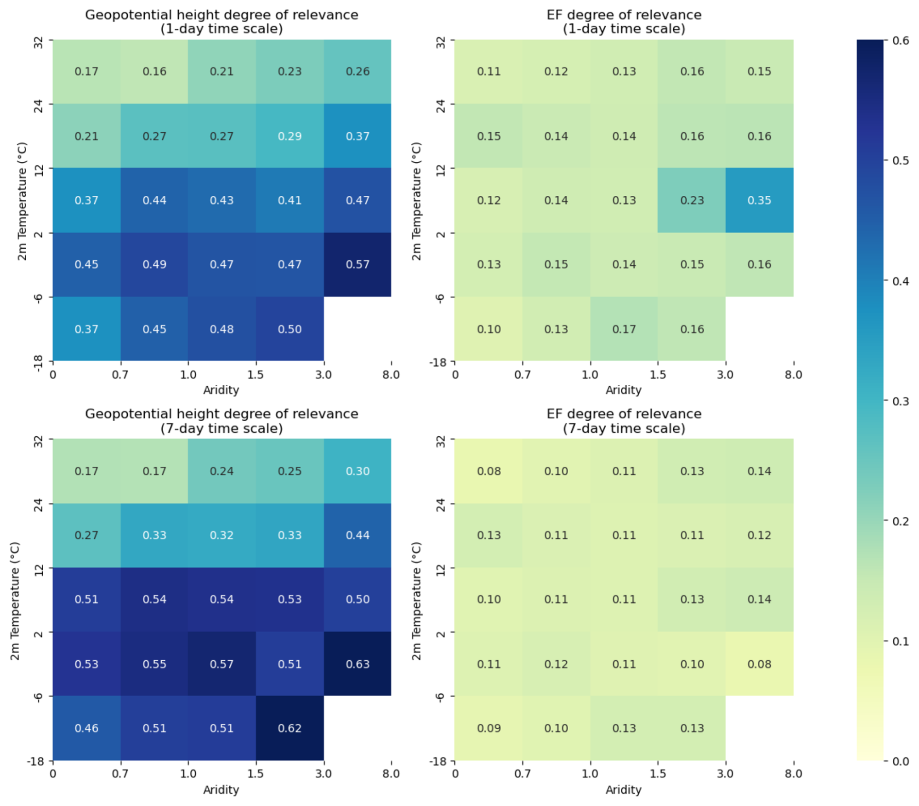
Figure A7 Geopotential height and EF median degree of relevance summarized across climate classes (given by aridity and temperature ranges) for 1 and 7 d hot extremes. White bins indicate regions that are masked out due to an insufficient number of grid cells (fewer than 20 grid cells).

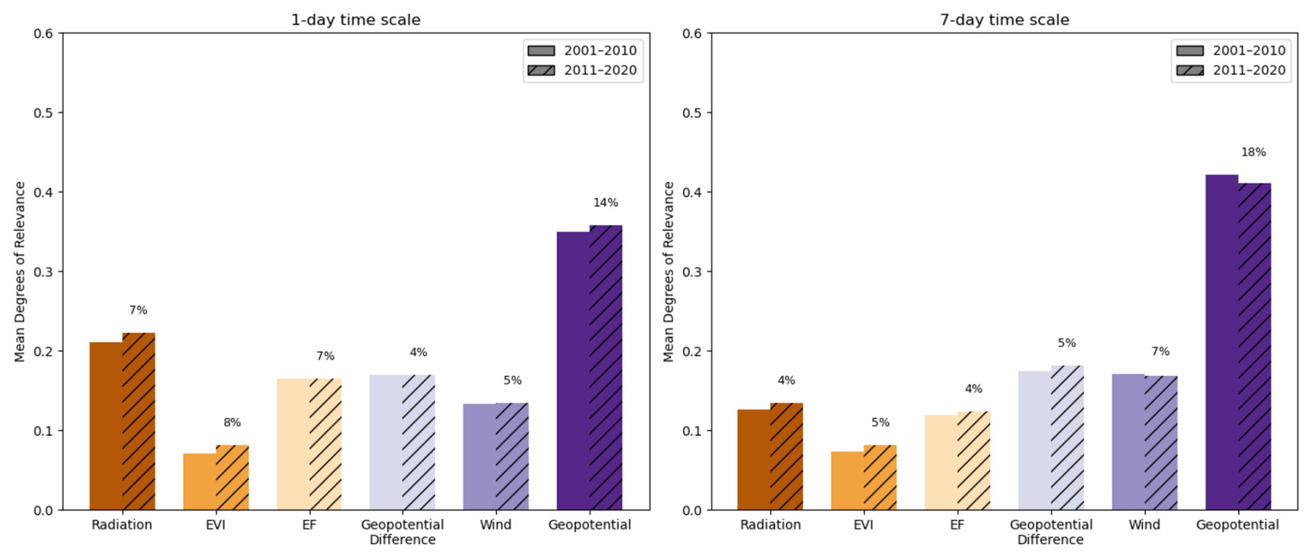
Figure A8 In light of the increasing trends in global temperature extremes (Seneviratne et al., 2023), we analyze potential changes in the relevance of the considered drivers of hot extremes over time. For this purpose, we divide the study period into two periods, 2001–2010 and 2011–2020, and employ the same methodology as described in Sects. 2.1–2.4 to calculate the relevance of all driver variables for each of the time periods. We also determine the significance of the changes in relevance through bootstrapping. For this purpose, we use the original 15 analogues (3 hot extremes × 5 analogues per hot extremes = 15 analogues) per grid cell and per time period (2001–2010 and 2011–2020) and draw a random sample of 15 from them (with replacement). Resampling is done 1000 times. Then, we compare the mean degrees of relevance of the resampled 15 analogues from both periods per grid cell such that we can infer significance from analyzing whether a substantial fraction (e.g., 950 out of the 1000) of the mean degrees of relevance between the two time periods is consistently above or below zero. This figure shows the changes in the mean degree of relevance of the hot extreme drivers considered across the study area between the first and second half of the study period. Bars without hatching denote results for the first half, and bars with hatching show results for the second half. The percentage above each pair of bars indicates the area-weighted fraction of grid cells where driver relevance changed significantly between both decades according to a bootstrap test for significant differences in means with a p value of 0.05

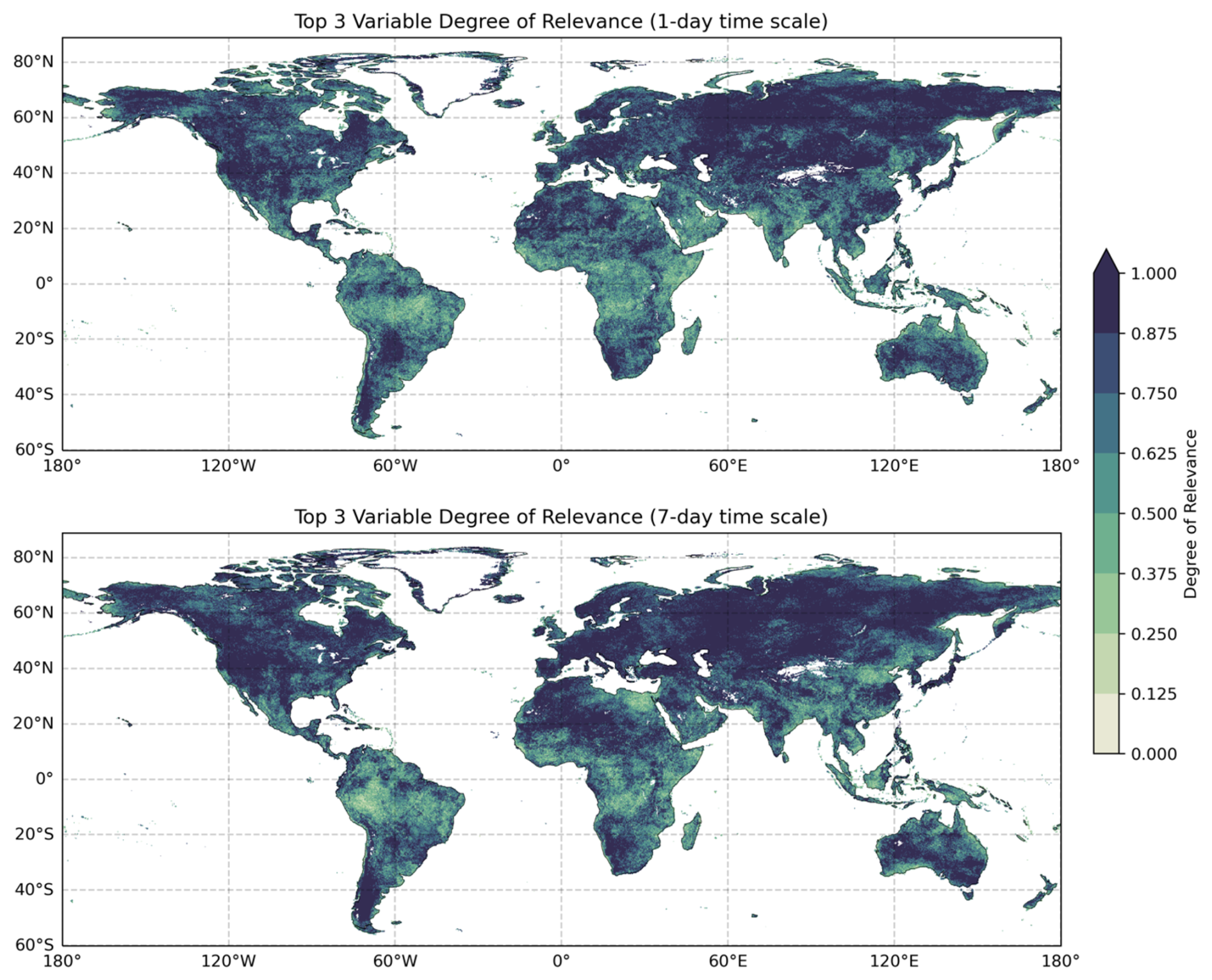
Figure A9 The sum of the degree of relevance of the three most influential variables for 1 and 7 d hot extremes. White indicates ocean/inland water or grid cells with insufficient data.

Table A1 A summary of the combined percentages of all variables from Fig. A4 in a tabular format. Detailed dominant driver variables are identified for 1 and 7 d hot extremes. Percentages represent the area where each driver is most influential.