ESD Ideas: Near-real-time preliminary detection of carbon dioxide source and sink areas using a Laplacian filter

Savytska, Yana; Smolii, Viktor; Weitzel, Nils

doi:https://doi.org/10.5194/esd-16-721-2025

Articles | Volume 16, issue 3

https://doi.org/10.5194/esd-16-721-2025

Special issue:

ESD Ideas

https://doi.org/10.5194/esd-16-721-2025

Articles | Volume 16, issue 3

ESD Ideas

28 May 2025

ESD Ideas |

| 28 May 2025

ESD Ideas: Near-real-time preliminary detection of carbon dioxide source and sink areas using a Laplacian filter

Yana Savytska, Viktor Smolii, and Nils Weitzel

Abstract

The constant rise in atmospheric CO₂ concentrations is warming the planet and causing climate change. Here, we propose digital filtration with a Laplacian filter for preliminary detection of areas with different changes in the characteristics of natural processes, using CO₂ sinks and sources as an example. This approach may improve CO₂ monitoring capabilities and enable near-real-time detection of CO₂ sources and sinks.

Download & links

Article (PDF, 1034 KB)

Download & links

How to cite.

Received: 28 Jun 2024 – Discussion started: 25 Jul 2024 – Revised: 11 Dec 2024 – Accepted: 11 Mar 2025 – Published: 28 May 2025

Over the past few decades, anthropogenic greenhouse gas (GHG) emissions have led to clearly detectable surface warming (IPCC, 2023). The major part – 75 % of all GHGs (Xiao et al., 2016) – is atmospheric carbon dioxide (CO₂). Our primary research, therefore, focuses on the development of a new method for CO₂ reduction. As part of this method, we propose an algorithm for the near-real-time preliminary detection of CO₂ source and sink areas. This algorithm can help to facilitate the monitoring, reporting, and verification of CO₂ source and sink areas. This includes the identification of an area as a CO₂ source or sink and its localization. We test the proposed algorithm using two types of CO₂ data measured at the near-surface layer. We applied digital filtration (Burger and Burge, 2016) to a CO₂ concentration (CDC) dataset to detect sink and source areas and CO₂ flux data to verify the results. Identifying the type of area as a CO₂ sink or source could help to improve the usability and functionality of CO₂ monitoring services, e.g., the Copernicus Atmosphere Monitoring Service and the NASA Carbon Monitoring System, or to assess the role and efficiency of different ecosystems in the global carbon cycle.

Applying digital filtration to CO₂ sink and source preliminary detection can be challenging due to their nature and behavior. Industrial objects have more stable emission characteristics. Natural objects have a clear seasonal and also daily periodic dependence. This leads to the need for continuous observations in near-real-time mode. Another potential challenge for satellite datasets is the technical limitation in the resolution of satellite datasets (the resolution of a sensor), which indirectly challenges the preliminary detection. At the current stage of our work, we do not focus on the factors that may affect the accuracy of detection but aim to explore the ability of digital filters to capture and detect changes in various characteristics of natural processes, for example, for the preliminary detection of CO₂ sinks and sources.

The response of an ecosystem to external and internal disturbances is reflected in the carbon balance (CB) of its sources and sinks (Xiao et al., 2016). Recent studies have described ecosystem responses to disturbances using functional indices – normalized difference vegetation index (Liu et al., 2022), net primary productivity, gross primary productivity (Mahecha et al., 2022), solar-induced fluorescence (Li et al., 2022) biodiversity (Mahecha et al., 2022), and others – in complex multivariate models (Holm et al., 2023). This makes them potentially accurate but also more resource-intensive, less straightforward, and less sensitive to short-term changes. Therefore, we propose the CDC as an integral parameter for the near-real-time detection of CO₂ sources and sinks that can also be applied to long-term observations.

Existing CO₂ monitoring services provide spatially distributed CDC on a global scale (Weir et al., 2022; CAMS, 2020). This does not include the detection of local CO₂ sink and source areas. A possible solution could be edge detection using digital filtration. This could sharpen the boundaries and make it possible to detect the CO₂ sink and source areas with a size corresponding to the resolution of the CDC dataset. Digital filtration is a well-known tool also used in geosciences, for example, to detect plumes of burning biomass (Goudar et al., 2023). In our paper, we do not quantify CO₂ sources and sinks because quantification is valuable for understanding the consequences of CO₂ changes after these changes have occurred. Our focus is on short-term (e.g., hours) CO₂ changes, which can help detect CO₂ sources and sinks and their different phases of development in near-real time until further analyses can be performed.

Before applying digital filtration, we need to consider the size of the areas, the characteristics of the internal physical, chemical, and biological processes, and the CB of each area. We work with the concept of a “small area” as a cell whose size depends on the inertia rate of chemical and physical processes and interpret it as a closed ecosystem based on the characteristics described below. Here the term small area is an analog of “small ecosystem”, defined by a set of characteristics and their values that describe an ecosystem in all its parts with a slight (or within the specified range) deviation. This deviation can be neglected at any time and at any place within the ecosystem.

The carbon balance can be seen as a strictly hierarchical system in which lower-level subsystems separately describe the CB in terms of its environmental and other conditions. The components of the subsystems are spatially distributed, defining the unique set of components of each area and determining the variability of environmental characteristics in different areas. To identify fluxes in the upper-atmospheric CB, we use two principles. The first is the direction of CO₂ flows (suffixes “In” and “Src” into the atmosphere or “Out” and “Sink” out of it). The second principle is relative to the boundary of the area – the prefix “Env” for the external environment and “Int” for internal processes and objects. Accordingly, we describe the total CB of the area of interest with Eq. (1):

\begin{matrix} (1) & CB = EnvIn - EnvOut + \sum {IntSrc}_{k} - \sum {IntSink}_{l}, \end{matrix}

where EnvIn is the flux intensity of the CO₂ injection from the external environment, EnvOut is the flux intensity of the CO₂ emission to the external environment, ∑IntSrc_k is the total flux intensity of internal CO₂ sources, and ∑IntSink_l is the total flux intensity of internal CO₂ sinks.

The external components of CB and their effects are independent of the characteristics of the area of interest, unlike the internal components. The internal components of the CB clearly correspond to the components of the ecosystem – plants of certain species, soil, etc. This balance defines the total amount of CO₂ in the atmosphere of the area and consequently the CDC = Func(CB).

The process of gas injection is inertial. For example, CO₂ emissions from a power plant do not change the CDC in every part of the Earth's atmosphere; they only affect the neighboring areas, and even then, it happens slowly, over some time. This process is described by diffusion and environmental conditions. We assume that the CDC in a small area that was formed at some earlier time does not change significantly during the time it takes the satellite to measure the CDC in neighboring small areas, and we interpret a data acquisition as a “monochrome image snapshot” of data.

The next two characteristics are also relevant to the definition of small area. Firstly, the characteristics of physical and chemical inertness in the atmosphere and soils will lead to different spatial distributions of the characteristics, and the speed of these processes will affect the size of the cells by considering the value limit of the specified deviation. Secondly, in digital filtration, the size of the cells processed must be the same, which is limited by the size of the smallest area of the system. Another filtration requirement concerns the presence and location of neighboring areas around the area of interest. According to the mathematical rules of sliding filtration (Aubry et al., 2014), cells should be located close to each other and partially have common boundaries, as shown in Fig. 1a. This requirement also leads to the neglect of air mass transport, as the short distances between the area of interest and neighboring areas minimize its impact – transferred external air masses will give approximately the same EnvIn and EnvOut components in all neighboring areas (in the filter focus). The small size and close location of cells also make it possible to detect the influence of external factors with synchronous changes in the monitored parameter with equal or proportional values (Fig. 1b).

https://esd.copernicus.org/articles/16/721/2025/esd-16-721-2025-f01

Figure 1Spatial and temporal CDC changes.

Download

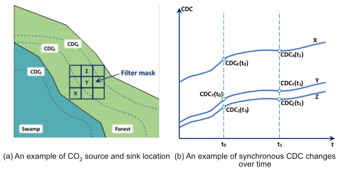
For example, at t₀, we expect different concentrations at points X, Y, and Z – CDC_X(t₀), CDC_Y(t₀), and CDC_Z(t₀), respectively – and assume that concentrations are related according to inequality (Eq. 2):

\begin{matrix} (2) & \begin{aligned} {CDC}_{X} (t_{1}) & > {CDC}_{X} (t_{0}) {CDC}_{Y} (t_{1}) \\ > {CDC}_{Y} (t_{0}) {CDC}_{Z} (t_{1}) \\ > {CDC}_{Z} (t_{0}) . \end{aligned} \end{matrix}

Inequality (Eq. 2) can be explained by natural processes – continuous changes in temperature, humidity, and other characteristics that lead to changes in the CO₂ emissions, e.g., from a swamp (Fig. 1a) – and corresponding changes in the CO₂ concentration in neighboring forest areas. Distance from the source and wind direction also affect the concentration. The time step for observing changes in CO₂ concentrations is 3 h in the selected dataset.

If, at t₁>t₀, the concentrations change according to Eq. (2) while all internal environmental conditions remain stable, this will result in a simultaneous multi-point (X–Z) increase in CDC as shown in Eq. (3):

\begin{matrix} (3) & \begin{aligned} Δ {CDC}_{X} ≃ Δ {CDC}_{Y} ≃ Δ {CDC}_{Z}, where \\ Δ {CDC}_{X, Y, Z} = {CDC}_{X, Y, Z} (t_{1}) - {CDC}_{X, Y, Z} (t_{0}) . \end{aligned} \end{matrix}

Equations 1–3 describe the connectivity and synchronicity of concentration change processes, but not their randomness. For example, Eq. (3) describes a synchronous increase in concentration due to daytime solar radiation based on the conditions outlined in Eq. (3).

\begin{matrix} (4) & \begin{aligned} {CDC}_{X} (t_{0}) & < {CDC}_{X} (t_{1}) {CDC}_{Y} (t_{0}) \\ < {CDC}_{Y} (t_{1}) {CDC}_{Z} (t_{0}) \\ < {CDC}_{Z} (t_{1}) \end{aligned} \end{matrix}

The above relationships and assumptions lead us to the conclusion that the CO₂ deltas shown in Eq. (4) correspond to the synchronous CDC changes for the whole area under the influence of external environmental conditions.

Based on Eq. (1), the difference between the CBs for two small neighboring ecosystems can be described by Eq. (5):

\begin{matrix} (5) & \begin{aligned} {CB}_{1} - {CB}_{2} \\ = ({EnvIn}_{1} - {EnvOut}_{1} + \sum {IntSrc}_{k 1} - \sum {IntSink}_{l 1}) \\ - ({EnvIn}_{2} - {EnvOut}_{2} + \sum {IntSrc}_{k 2} - \sum {IntSink}_{l 2}) . \end{aligned} \end{matrix}

According to the concept of small neighboring areas, the values of EnvIn and EnvOut are equal in all cells, and therefore the result of Eq. (5) can be interpreted as the difference in CO₂ fixation efficiency with Eq. (6):

\begin{matrix} (6) & \begin{aligned} {CB}_{1} - {CB}_{2} & = (\sum {IntSrc}_{k 1} - \sum {IntSink}_{l 1}) \\ - (\sum {IntSrc}_{k 2} - \sum {IntSink}_{l 2}) . \end{aligned} \end{matrix}

If the characteristics of the neighboring ecosystems are similar (each of the IntSrc_k1 sources of the first area is equal to IntSrc_k2 in the second neighboring area, and each IntSink_l1 is equal to IntSink_l2), then based on Eq. (6) it is possible to identify the emergence of the external CO₂ source according to Eq. (7):

\begin{matrix} (7) & {CB}_{1} - {CB}_{2} = ({EnvIn}_{1} - {EnvOut}_{1}) - ({EnvIn}_{2} - {EnvOut}_{2}) . \end{matrix}

Each ecosystem is surrounded by neighboring ecosystems, which can be represented in the Cartesian coordinate system with a set of indices in the vertical, horizontal, and diagonal directions.

\begin{matrix} (8) & |\begin{array}{ccc} 4 & 3 & 2 \\ 5 & 0 & 1 \\ 6 & 7 & 8 \end{array}| \end{matrix}

When we form the convolutional filter of the difference between the central element and a given element, the coefficient 1 is placed in the center of the matrix (zero index) and the coefficient −1 is in the position defined by a given index. Using this indexing system and the convolutional filter principle, the difference (Eq. 5) can be described in a matrix operation form over CB data as follows.

\begin{matrix} (9) & \begin{aligned} F (CB) & = ({CB}_{1} - {CB}_{2}) \Rightarrow (1 \times {CB}_{1} + (- 1) \times {CB}_{2}) \\ \Rightarrow |\begin{array}{ccc} 0 & 0 & - 1 \\ 0 & 0 & 1 \\ 0 & 0 & 0 \end{array}| \end{aligned} \end{matrix}

The central index corresponds to the area of interest, and the rest are neighboring areas. The matrix for evaluating the difference between all eight neighboring cells is as follows.

\begin{matrix} (10) & \begin{aligned} F (CB) & = \sum_{i = 1}^{i = 8} ({CB}_{0} - {CB}_{i}) \\ \Rightarrow \nabla (CB) = |\begin{array}{ccc} - 1 & - 1 & - 1 \\ - 1 & 8 & - 1 \\ - 1 & - 1 & - 1 \end{array}| \end{aligned} \end{matrix}

The area of interest is identified as a CO₂ sink or source based on its CDC in relation to that of the neighboring areas. This means that the resolution of the dataset and the number of neighboring areas define the area of identification. Depending on the expected sizes of CO₂ sinks and sources, the resolution of the dataset and the size of the matrix of coefficients can be adjusted. This option shows the universality of the proposed algorithm with respect to the sizes of CO₂ sources and sinks.

This matrix corresponds to the Laplacian convolutional filter. This is a second-order filter used for edge detection and feature extraction (Aubry et al., 2014). Unlike first-order filters, we do not need separate filters to detect and then combine vertical and horizontal edges, as the Laplacian filter detects all edges regardless of direction.

In order to apply the Laplacian filter to a CDC dataset formed by carbon balances, we performed a convolution operation, which mathematically means a combination of two matrices, in our case one containing the CDCs and the other the filter coefficients. The convolution operation, represented by Eq. (11), involves sliding the filter over the dataset, multiplying the CDCs by the corresponding coefficients, and adding them up. The result is a new dataset of the same size as the original, but the calculated CDC differences can be positive, negative, or zero. A positive value after digital filtration means that the original CDC in the area of interest is greater than the average CDC in the neighboring areas. This area is identified as containing the CO₂ source. Conversely, an area with a negative value is identified as containing a CO₂ sink. A zero value indicates CO₂ homogeneous areas.

\begin{matrix} (11) & \begin{aligned} {CDC}_{filtered} & = [\begin{array}{ccc} {CDC}_{4} & {CDC}_{3} & {CDC}_{2} \\ {CDC}_{5} & {CDC}_{0} & {CDC}_{1} \\ {CDC}_{6} & {CDC}_{7} & {CDC}_{8} \end{array}] \\ \times [\begin{array}{ccc} - 1 & - 1 & - 1 \\ - 1 & 8 & - 1 \\ - 1 & - 1 & - 1 \end{array}] \end{aligned} \end{matrix}

This filter, with a size of 3×3 cells, covers the area of 4.8×6.6 km when scanned with OCO satellites (Orbiting Carbon Observatory, 2015). It is optimal for our task in terms of processing time and computational complexity – 15 arithmetic operations for an area of interest – and does not require additional computational resources. This partially provides real-time computation for the six areas in the satellite scan area strip, which requires 90 operations per second.

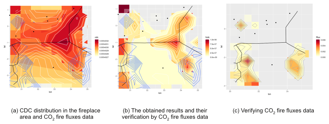
The test results of the proposed algorithm (Appendix A) for CO₂ source and sink area detection show that it is sufficient for a rapid-fire response or for a detailed subsequent study of the CO₂ fixation characteristics of the vegetation in the sink area. We do not consider CO₂ advection for the source area detection because the influence of air mass transport is small. It is close to 6 % at a wind speed of 30 m s⁻¹ and a scanning time of three data rows by satellite for 1 s (Orbiting Carbon Observatory, 2015). This value is applicable for the tasks of rough CO₂ source and sink area detection.

Appendix A: Results of CO₂ source and sink area detection with a Laplacian filter

According to the proposed method, the preliminary detection of CO₂ sources and sinks involves the following steps: (1) digital filtration of the CO₂ concentrations in the area of interest and identification of the area as a source or sink by the sign (+ is a source, − is a sink), (2) comparison of the superimposed filtered CO₂ concentrations with fire fluxes in the area of interest, and (3) finding the area where two parameters are closely superimposed at their maximum intensities.

To test the proposed algorithm with a CO₂ source area detection, we chose a large fire event in the Serengeti National Park, Tanzania, which started on 22 July 2016 and lasted for 31 d. We used CDC values as an indicator of a fire area and CDC spatial differences to detect area boundaries. For the experiment, we took the CDCs for 27 July 2016 (Weir et al., 2022), the fifth day after the fire had started, to avoid the influence of additional CO₂ from a previous fire event in the area. The CDC distribution for this date is shown in Fig. A1a, but it is not possible to see the clear boundaries of the area because the spatial CDC differences are blurred. In order to detect the fire area boundaries, we applied the Laplacian filter, assuming that all the CDCs in the area were measured at the same time. The results are shown in Fig. A1b, where each cell has a different shading, representing a change in CDC intensity. The dark shaded cells are defined as CO₂ sources.

https://esd.copernicus.org/articles/16/721/2025/esd-16-721-2025-f02

Figure A1Spatial distributions of the CO₂ parameters and the obtained results of the CO₂ source area detection.

Download

https://esd.copernicus.org/articles/16/721/2025/esd-16-721-2025-f03

Figure A2Spatial distributions of filtered CDC and vegetation indices for CO₂ sink area detection.

To verify the obtained results, we compared them with CO₂ fire flux data for the aboveground layer that contains daily fire emissions from 2003 to 2017 (Ott, 2020). These data are presented in Fig. A1c, which shows the CO₂ fire flux rate with color intensity and isolines, and in Figs. A1a and A1b with isolines only. The density of the isolines is related to the rate of flux intensity change – higher density corresponds to a higher rate, and lower density corresponds to a lower rate of change. The spatial resolutions of the CDC dataset and the CDC flux dataset are different at 1°×1° and 0.5°×0.5°, respectively. Different resolutions pose a challenge for source validation, so we use a graphical image overlay with a relative placement by the object coordinates for preliminary detection.

The greater the number of isolines around the point, the faster the concentration changed. The comparison of the experimental results and the flux data showed rough agreement in the detection of the CO₂ source area. The differences in location can be explained by the higher spatial resolution of the flux data. However, the process of obtaining flux data requires either a complex information model that is not real-time or a satellite to fly over the same point on Earth at least twice. In situations that require a more operational response, such as the start of a large forest fire near a populated area or an emergency at a power plant with high CO₂ emissions, this may be too long. In our experiment, we chose available CDC data, interpreted as “at the moment”, and applied a Laplacian filter to detect CO₂ source areas. In reality, the proposed method can be applied to the satellite-scanned data “strip” in real time.

Identifying areas that are CO₂ sinks is different from identifying areas that are short-term sources of CO₂. The most important terrestrial CO₂ sink is vegetation, the characteristics of which depend mainly on the time of day and the season. The size of large forests does not change over hours or days but over years or decades. We, therefore, need to define the boundaries of large forests once and then monitor them.

For our experiment, we chose CDC data (CAMS, 2020) for the period of active vegetation growth and analyzed data for Alaska in June 2016. We considered land cover (LC) type, biomass, and growth phase (NDVI) as parameters of CO₂ fixation. First, we compared the CDC data processed with the Laplacian filter (Fig. A2a) with the LC types in Alaska. The results of this comparison are shown in Fig. A2b, where the LC data are presented in the FAO Land Cover Classification System (LCSS) (Friedl and Sulla-Menashe, 2019). The isolines in the figure show the change in CDC intensity, which roughly corresponds to the formal boundaries of the LCCS vegetation classes. Forests with more than 60 % tree cover (Di Gregorio, 2005) – evergreen forests, deciduous forests, and mixed forests – show a higher CO₂ fixation.

In contrast, there is little spatial difference in CO₂ fixation between the areas covered by shrubs and herbs in Fig. A2b, possibly due to the small amount of biomass in these ecosystems and the potential influence of the nearby ocean.

The filtered CDC is nearly negligible on the mountaintops due to the uniform barren ground, ice, and snow zones. The NDVI (Fig. A2c) is also less significant in these areas. In contrast, the central part of Alaska, which is covered by a large amount of evergreen biomass with high NDVI (Didan, 2020) is identified as a CO₂ sink. Mountains protect this area from the influence of the oceans. These results could help in further work to explain the different CO₂ fixation potentials in different subregions of these areas based on the absolute values of processed CDCs.

Code and data availability

Data and code are available from Zenodo at https://doi.org/10.5281/zenodo.12532657 (Savytska and Smolii, 2024).

Author contributions

YS conceptualized the study and designed the method with contributions from VS and NW. YS and VS processed the data. YS wrote the paper. All authors participated in reviewing and discussing the paper.

Competing interests

The contact author has declared that none of the authors has any competing interests.

Disclaimer

Publisher's note: Copernicus Publications remains neutral with regard to jurisdictional claims made in the text, published maps, institutional affiliations, or any other geographical representation in this paper. While Copernicus Publications makes every effort to include appropriate place names, the final responsibility lies with the authors.

Acknowledgements

This research was carried out as part of the “Research@Tübingen” fellowship and an individual project of Yana Savytska within the Philipp Schwartz postdoctoral program. Nils Weitzel was supported by the Engineering and Physical Sciences Research Council (EPSRC, grant number EP/Z002591/1). The authors thank two anonymous reviewers and the editor, Min Chen, for the constructive feedback and editorial work.

Financial support

This open-access publication was funded by the Open Access Publication Fund of the University of Tübingen.

Review statement

This paper was edited by Min Chen and reviewed by two anonymous referees.

References

Aubry, M., Paris, S., Hasinoff, S. W., Kautz, J., and Durand, F.: Fast Local Laplacian Filters: Theory and Applications, ACM Trans. Graph., 33, 167, https://doi.org/10.1145/2629645, 2014.

Burger, W. and Burge, M. J.: Digital Image Processing: An Algorithmic Introduction. Digital Image Processing, 2nd Edn., Springer Nature, London, XXIII, 811 pp., https://doi.org/10.1007/978-1-4471-6684-9, 2016.

CAMS: Global inversion-optimised greenhouse gas fluxes and concentrations, Copernicus Atmosphere Data Store [data set], https://ads.atmosphere.copernicus.eu/datasets/cams-global-greenhouse-gas-inversion?tab=overview (last access: 1 May 2024), 2020

Didan, K.: MODIS/Terra Vegetation Indices 16-Day L3 Global 500 m SIN Grid, Land Processes Distributive Active Archive Center [data set], https://lpdaac.usgs.gov/products/mod13a1v061/ (last access: 20 June 2024), 2020.

Di Gregorio, A.: Land cover classification system: classification concepts and user manual: LCCS, Number 8, Food and Agriculture Organization, Rome, Italy, ISBN 92-5-104216-0, https://www.fao.org/4/x0596e/x0596e00.htm (last access: 1 May 2024), 2005.

Friedl, M. and Sulla-Menashe, D.: MCD12Q1 MODIS/Terra+Aqua Land Cover Type Yearly L3 Global 500m SIN Grid V006, NASA EOSDIS Land Processes Distributed Active Archive Center [data set], https://doi.org/10.5067/MODIS/MCD12Q1.006, 2019.

Goudar, M., Anema, J. C. S., Kumar, R., Borsdorff, T., and Landgraf, J.: Plume detection and emission estimate for biomass burning plumes from TROPOMI carbon monoxide observations using APE v1.1, Geosci. Model Dev., 16, 4835–4852, https://doi.org/10.5194/gmd-16-4835-2023, 2023.

Holm, J. A., Medvigy, D. M., Smith, B., Dukes, J. S., Beier, C., Mishurov, M., Xu, X., Lichstein, J. W., Allen, C. D., Larsen, K. S., Luo, Y., Ficken, C., Pockman, W. T., Anderegg, W. R. L., and Rammig, A.: Exploring the impacts of unprecedented climate extremes on forest ecosystems: hypotheses to guide modelling and experimental studies, Biogeosciences, 20, 2117–2142, https://doi.org/10.5194/bg-20-2117-2023, 2023.

IPCC: Summary for Policymakers, in: Climate Change 2023: Synthesis Report, Contribution of Working Groups I, II and III to the Sixth Assessment Report of the Intergovernmental Panel on Climate Change, edited by: Core Writing Team, Lee, H., and Romero, J., IPCC, Geneva, Switzerland, 1–34, https://doi.org/10.59327/IPCC/AR6-9789291691647.001, 2023.

Li, C., Peng, L., Zhou, M., Wei, Y., Liu, L., Li, L., Liu, Y., Dou, T., Chen, J., and Wu, X.: SIF-Based GPP Is a Useful Index for Assessing Impacts of Drought on Vegetation: An Example of a Mega-Drought in Yunnan Province, China, Remote Sens., 14, 1509, https://doi.org/10.3390/rs14061509, 2022.

Liu, L., Jiang, Y., Gao, J., Feng, A., Jiao, K., Wu, S., Zuo, L., Li, Y., and Yan, R.: Concurrent Climate Extremes and Impacts on Ecosystems in Southwest China, Remote Sens., 14, 1678, https://doi.org/10.3390/rs14071678, 2022.

Mahecha, M. D., Bastos, A., Bohn, F. J., Eisenhauer, N., Feilhauer, H., Hartmann, H., Hickler, T., Migliavacca, M., Otto, F. E., Peng, J., Quaas, J., Tegen, I., Weigelt, A., Wendisch, M., and Wirth, C.: Biodiversity loss and climate extremes – Study the feedbacks, Nature, 612, 7938, https://doi.org/10.1038/d41586-022-04152-y, 2022.

Orbiting Carbon Observatory (OCO): Algorithm Theoretical Basis Document (ATBD), National Aeronautics and Space Administration https://docserver.gesdisc.eosdis.nasa.gov/public/project/OCO/OCO_L2_ATBD.pdf (last access: 1 May 2024), 2015.

Ott, L.: GEOS-Carb CASA-GFED Daily Fire and Fuel Emissions 0.5°×0.5°, V2, Greenbelt, MD, USA, Goddard Earth Sciences Data and Information Services Center (GES DISC) [data set], https://doi.org/10.5067/IYZIZJ8ZFZHU, 2020.

Savytska, Y. and Smolii, V.: Test Datasets (CDC, Fire Fluxes, Land Cover and shapefiles) and code (1.0.0), Zenodo [data set and code], https://doi.org/10.5281/zenodo.12532657, 2024.

Weir, B., Ott, L., and OCO-2 Science Team: OCO-2 GEOS Level 3 daily, 0.5×0.625 assimilated CO₂ V10r, Greenbelt, MD, USA, Goddard Earth Sciences Data and Information Services Center (GES DISC) [data set], https://doi.org/10.5067/Y9M4NM9MPCGH, 2022.

Xiao, J., Liu, S., and Stoy, P. C.: Preface: Impacts of extreme climate events and disturbances on carbon dynamics, Biogeosciences, 13, 3665–3675, https://doi.org/10.5194/bg-13-3665-2016, 2016.

Articles

Short summary

In recent decades, we have witnessed abnormally hot summers and frequent weather extremes globally. These are clear signs of global warming and climate change. A constant increase in atmospheric carbon dioxide (CO₂) is a major driver of these changes. We propose an algorithm for near-real-time detection of terrestrial areas with CO₂ sources and sinks. This algorithm could aid in developing new methods of natural CO₂ reduction and exploring ecosystem responses to disturbances.