Impact of Greenland Ice Sheet disintegration on atmosphere and ocean disentangled

We analyze the impact of a disintegrated Greenland Ice Sheet (GrIS) on the climate through steady-state simulations with the global Max Planck Institute for Meteorology Earth System Model (MPI-ESM). This advances our understanding of the intricate feedbacks between the GrIS and the full climate system. Sensitivity experiments enable the quantification of the individual contributions of altered Greenland surface elevation and properties (e.g., land cover) to the atmospheric and oceanic climate response. Removing the GrIS results in reduced mechanical atmospheric blocking, warmer air temperatures over Greenland and thereby changes in the atmospheric circulation. The latter alters the wind stress on the ocean, which controls the ocean-mass transport through the Arctic gateways. Without the GrIS, the upper Nordic Seas are fresher, attenuating deep-water formation. In the Labrador Sea, deep-water formation is weaker despite a higher upper-ocean salinity, as the inflow of dense overflow from the Denmark Strait is reduced. Our sensitivity experiments show that the atmospheric response is primarily driven by the lower surface elevation. The lower Greenland elevation dominates the ocean response through wind-stress changes. Only in the Labrador Sea do altered Greenland surface properties dominate the ocean response, as this region stores excessive heat from the Greenland warming. The main drivers vary vertically: the elevation effect controls upper-ocean densities, while surface properties are important for the intermediate and deep ocean. Despite the confinement of most responses to the Arctic, a disintegrated GrIS also influences remote climates, such as air temperatures in Europe, the Atlantic Meridional Overturning Circulation (AMOC) and the subtropical gyre. These interactions and feedbacks between ice sheets and the other climate components highlight the necessity of including dynamic ice sheets in climate models that are used for future projections.

1 Introduction

Located between 60 and 85° N and characterized by steep topography with peaks exceeding 3000 m, the Greenland Ice Sheet (GrIS) is a prominent feature in the Northern Hemisphere that not only impacts the local climate (Box et al., 2012; Oerlemans and Vugts, 1993; van den Broeke et al., 1994), but also the remote climate (Lunt et al., 2004; Davini et al., 2015). In view of the present mass loss (Shepherd et al., 2020) and potential disappearance of the GrIS under ongoing anthropogenic global warming (Aschwanden et al., 2019), it is imperative to understand the interplay between GrIS characteristics and the broader climate system. A number of studies have investigated potential climatic effects of a completely or almost completely melted GrIS on the Northern Hemisphere Earth system under various climates. These studies found considerable climatic changes in response to a reduced GrIS volume, including thermodynamic changes in the climate over and in the vicinity of Greenland, such as a warming (Crowley and Baum, 1995; Davini et al., 2015; Dethloff et al., 2004; Hakuba et al., 2012; Junge et al., 2005; Lunt et al., 2004; Merz et al., 2014a; Ridley et al., 2005; Solgaard and Langen, 2012; Stone and Lunt, 2013; Toniazzo et al., 2004; Vizcaíno et al., 2008) and a redistribution in precipitation over Greenland (Davini et al., 2015; Dethloff et al., 2004; Lunt et al., 2004; Merz et al., 2014b; Solgaard and Langen, 2012; Stone and Lunt, 2013; Toniazzo et al., 2004; Petersen et al., 2004). Further studies found dynamic changes, such as an increase in cyclonic activity over Greenland (Toniazzo et al., 2004; Petersen et al., 2004; Junge et al., 2005; Davini et al., 2015) and a weakening of the Atlantic Meridional Overturning Circulation (AMOC) (Davini et al., 2015). However, a clear separation between the two primary effects of a disintegrated GrIS – lower surface elevation and altered surface properties (e.g., land cover) – and their respective contributions to the changed climate has yet to be established. The primary objective of the present study is to systematically analyze the interactions of the GrIS with the atmosphere and ocean, whereby we specifically focus on ocean dynamics.

Disentangling the impact of the two aforementioned effects on the atmosphere and ocean remained challenging, as (1) coupled atmosphere–ocean models with interactive ice sheets (Ridley et al., 2005; Vizcaíno et al., 2008) require the inclusion of a myriad of feedback mechanisms that complicate the attribution of simulated climate changes to specific processes and (2) ocean models require a long-enough model spin-up to equilibrate the deep ocean, which is computationally demanding. Hence, most previous studies restricted their analysis of the impact of modified GrIS surface elevation and surface properties on the climate system to the interaction with the atmosphere, using prescribed sea-surface temperature (SST) and sea-ice conditions (Crowley et al., 1994; Crowley and Baum, 1995; Dethloff et al., 2004; Hakuba et al., 2012; Junge et al., 2005; Kristjánsson and Mcinnes, 1999; Kristjánsson et al., 2009; Merz et al., 2014a, b; Petersen et al., 2004), or they only considered the response of the upper ocean by using a simplified ocean model (Lunt et al., 2004). Few studies also highlighted the importance of the GrIS surface elevation and properties under either pre-industrial (PI) or present-day conditions for the ocean system without using external freshwater forcing. Although these studies used a dynamic ocean component within a coupled Atmosphere—Ocean General Circulation Model (AOGCM) (Davini et al., 2015; Toniazzo et al., 2004), their analyses did not consider a long-enough model spin-up compared to the response timescales of the deep ocean. This constrains the exploration of interactions and feedbacks with the deep ocean. In addition to these limitations, the aforementioned studies lack a differentiation between the individual contributions of GrIS surface elevation and properties on the climate changes. Only Stone and Lunt (2013) conducted additional sensitivity experiments to separate between the two effects using a coupled AOGCM. However, their study is constrained to the analysis of atmospheric feedbacks. Similarly, Lunt et al. (2004) limited their analysis of individual contributions to air temperature differences. Lastly, most of the aforementioned studies focused on the climate impacts of a disintegrated GrIS on Greenland and the adjacent regions. Here, we expand upon those studies by examining the interactions of the GrIS with both the atmosphere and the ocean, including the deep ocean. Understanding these interactions is imperative, particularly in light of the recent accelerated mass loss of the GrIS under global warming. Further, we point towards the remote effects of a disintegrated GrIS, e.g., the impact on European temperatures.

To study the global climate response to a complete disintegration of the GrIS, we conducted a set of steady-state coupled atmosphere–ocean-dynamic–vegetation simulations, using the Max Planck Institute for Meteorology Earth System Model (MPI-ESM) with fixed ice sheets. We disentangle the individual contributions of the reduced GrIS surface elevation and altered surface properties by changing the GrIS height and extent as well as land cover between simulations. Additional sensitivity experiments allow us to separate between the feedback of the GrIS with the atmosphere and ocean. A multi-millennium spin-up until equilibrium allows for the analysis of the deep ocean. This approach enables us to complement previous studies by a systematic attribution of the effects of a disintegrated GrIS on the full global climate system.

The structure of this paper is as follows: in Sect. 2, we describe the model setup and the experimental design. Section 3 presents the implications of a disintegrated GrIS for the Earth system, starting with the feedback mechanisms between the GrIS and the atmosphere, followed by the interactions with the ocean. The last part of Sect. 3 quantifies the contribution to the discussed response of the Earth system by the altered GrIS surface elevation and surface properties. In Sect. 4, these findings are discussed with respect to previous findings, followed by a conclusion in Sect. 5.

2 Methods

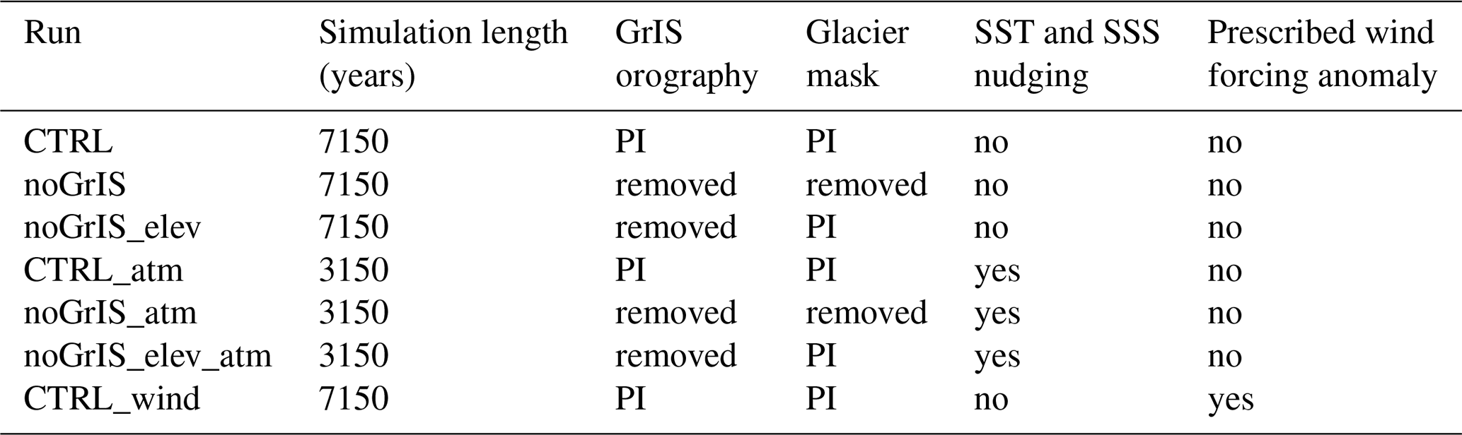
To investigate the climate response to different states of the GrIS, we conducted a systematic set of model simulations with MPI-ESM. The first three simulations differ in terms of their GrIS extent and height as well as the retention of their glacier mask. Additional experiments serve to understand the respective effects on the atmosphere and/or ocean and the feedback between these components. Table 1 gives an overview of all experiments.

2.1 Model system

For this study, we used MPI-ESM version 1.2 in a coarse resolution (Mauritsen et al., 2019). The model consists of the ECHAM6.3 spectral atmospheric model (Stevens et al., 2013) at a T31 horizontal resolution (approximately 3.75°) and 31 vertical levels, the JSBACH3.2 land surface vegetation model (Raddatz et al., 2007), and the MPIOM1.6 primitive equation ocean model (Marsland et al., 2003; Mikolajewicz et al., 2007) with a nominal resolution of 3°. For more details on the model system, refer to Kapsch et al. (2022).

2.2 Experimental design

All seven simulations were started from a simulation of the last deglaciation with prescribed ice sheets from ICE-6G reconstructions (ICE6G_P3, Kapsch et al., 2022; Peltier et al., 2015) at year 1840. The first simulation, hereafter named CTRL, is a reference simulation that resembles a steady-state PI simulation based on ICE6G_P3. For this simulation, we used the PI ice sheet with a maximum elevation of 3096 m in the central region of Greenland (Fig. 1a). Further, PI greenhouse gas concentrations (Köhler et al., 2017), insolation and orbital parameters (Berger and Loutre, 1991) were prescribed. In a second experiment, we removed the GrIS, which we refer to as noGrIS (Fig. 1b). noGrIS has the same boundary and initial conditions as CTRL, except for the Greenland orography, which was taken from a simulation with the fully coupled climate–ice-sheet–solid-earth model MPI-ESM-mPISM-VILMA. In this simulation, CO₂ concentrations follow the SSP5-8.5 emission scenario until the year 2500 (Meinshausen et al., 2020). After year 2500, CO₂ concentrations were taken from a CLIMBER simulation (Brovkin et al., 2012; Kleinen et al., 2021). This CO₂ forcing caused a complete disintegration of the GrIS under peak CO₂ values in the MPI-ESM-mPISM-VILMA simulation. For noGrIS, we replaced the GrIS orography with the underlying isostatically adjusted surface bedrock of the fully coupled simulation at the time when the GrIS has completely melted. In noGrIS, highest mountains are found in the eastern and southern regions of Greenland, with a maximum elevation of about 1320 m. We also removed the glacier mask (pink outline in Fig. 1a), allowing for the vegetation to dynamically regrow and surface parameters to change to those of a non-glaciated surface, including, for example, changes in the albedo, ground roughness and the ground heat flux. An overview of all the variables changed is given in Reick et al. (2021). While the model captures transitions in the vegetation, a comprehensive investigation of the feedbacks between changes in the vegetation and the climate system is out of the scope of this study. The impacts of all changes in the land cover and surface parameters are thus summarized as GrIS surface properties.

To disentangle the individual contributions of the reduced GrIS orography and the altered surface properties, we performed a third experiment. In this experiment, referred to as noGrIS_elev, we applied all the orographic changes as in noGrIS but maintained the surface properties in their original, glaciated state. For this, we kept the glacier mask constant, comparable to CTRL. Note that in none of the experiments was the freshwater associated with the removal of the GrIS added into the ocean, following previous approaches (Davini et al., 2015; Lunt et al., 2004; Stone and Lunt, 2013). The impact of the 7 m sea-level equivalent from the GrIS on ocean salinity would be less than 0.2 % and is thus negligible. This approach provides the advantage that we do not need to correct for differences in the global mean salinity when analyzing density changes, as it does not represent a climate change signal. Further, land–sea mask and river runoff directions were kept constant. The three main experiments were integrated for 7150 years. Equilibrium in the deep ocean emerges after approximately 4150 years in these simulations.

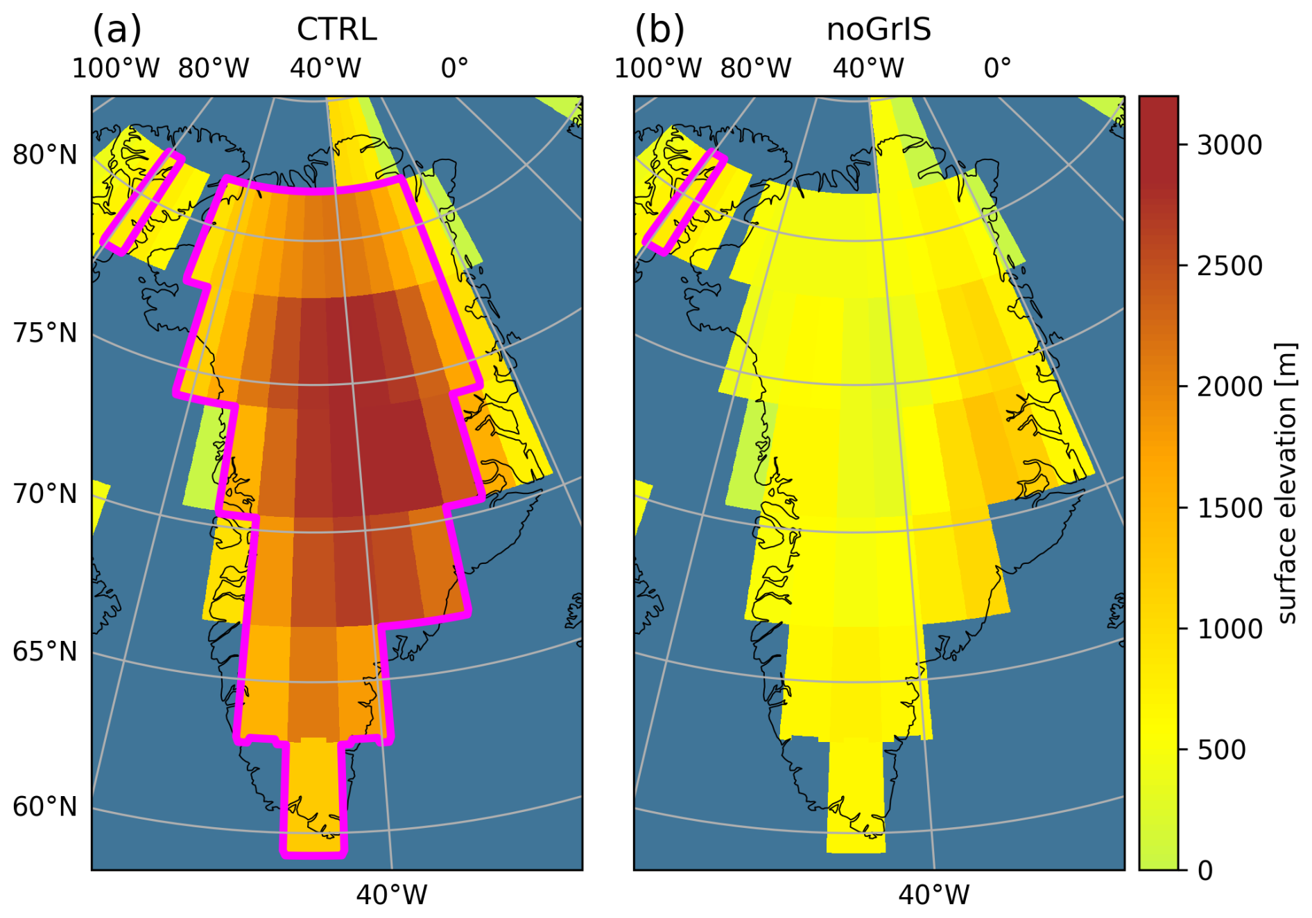
Figure 1 Surface elevation used as input to MPI-ESM for (a) CTRL and (b) noGrIS. The pink outline shows the glacier mask.

Four additional sensitivity experiments were performed to disentangle the respective impact of a disintegrated GrIS on the atmosphere and ocean. The first three experiments resemble CTRL, noGrIS and noGrIS_elev, but SST and sea-surface salinity (SSS) were nudged towards the climatology of the CTRL simulation. Hence, these experiments exclusively consider interaction of the GrIS with the atmosphere and sea ice, suppressing the ocean response. We interpret them as the atmospheric contribution to the full climate response. These simulations are referred to as CTRL_atm, noGrIS_atm and noGrIS_elev_atm, respectively. As the atmosphere needs less time to equilibrate than the ocean, the simulations were integrated for 3150 years to reach a steady state.

A last experiment, referred to as CTRL_wind, was conducted to shed light on the dynamical atmospheric effects of the GrIS height reduction on the ocean. For this experiment, we maintained the same conditions as in CTRL but imposed the wind-stress anomaly of the simulation in which we only consider atmospheric changes in response to the elevation reduction (noGrIS_elev_atm) and CTRL_atm.

For the analysis, the final 1000 years of each simulation were averaged, and all experiments are compared to their respective control experiment. For the atmosphere, we focus our analysis on the winter season (DJF), as largest atmospheric changes in the Northern Hemisphere occur during these months. Given that the ocean responds on longer timescales than the atmosphere, our ocean and wind-stress analysis is based on annual-mean values.

Table 1 Overview of the performed experiments, including simulation length, GrIS orography (PI extent or removed GrIS), GrIS surface properties (PI or no glacier mask), and whether nudging (SST and SSS) or the application of a wind-stress anomaly flux correction from the noGrIS_elev_atm experiment was applied.

3 Results

The implications of a disintegrated GrIS for the Earth system are analyzed in the following. In Sect. 3.1, we explore the atmospheric response and in Sect. 3.2 the ocean response to an absent GrIS. Section 3.4 provides a comprehensive overview of the chain of effects and contributions of the lower GrIS surface elevation and properties on the climate.

3.1 Atmosphere response

The analysis of the atmospheric response to a disintegrated GrIS is split into three parts. The first part describes the spatial and seasonal patterns of the 2 m air temperature response. The second part looks into the atmospheric processes driving the formerly described difference. The last part attributes the 2 m air temperature changes over Greenland to their respective drivers and quantifies them.

3.1.1 Near-surface air temperature response

In CTRL, the Northern Hemisphere annual-mean 2 m air temperature is 286.6 K (13.5 °C), whereby Greenland experiences considerably colder conditions, with an average temperature of 254.6 K (−18.6 °C). The colder conditions are a result of the unique geographical characteristics of the GrIS, including its high elevation, latitudinal position and vast glaciated area, characterized by a highly reflective surface.

Winter

Removing the orography of the GrIS leads to a strong warming over Greenland: the spatially averaged winter 2 m air temperature over Greenland is 7.9 K warmer in noGrIS than in CTRL, with a local maximum of 16.0 K (Fig. 2a). Across the Arctic region, a pronounced dipole pattern emerges in the winter 2 m air temperature difference. Specifically, warmer temperatures are depicted in the western Arctic in noGrIS compared to CTRL, with a maximum across Greenland. In contrast, the eastern Arctic experiences up to 6.0 K colder conditions in noGrIS than in CTRL, particularly over the Nordic Seas, the Barents Sea and northern Europe. This dipole pattern is also reflected in the SST and the sea-ice extent, as they are directly altered by the overlying atmosphere – a connection that is further explored in Sect. 3.2.

The experiments with a nudged ocean (noGrIS_atm and noGrIS_elev_atm) reveal that the temperature dipole results from changes in the atmospheric circulation in response to the lowered GrIS surface elevation (Fig. 2b and c). Figure 2f shows that ocean feedbacks lead to an exclusively negative temperature response in the Arctic. Positive temperature anomalies in the ocean are observed only south of the Arctic Circle, specifically over the Labrador Sea, but not over the Canadian Arctic Archipelago and northern Canada. Hence, they cannot be the driver of the temperature dipole pattern. In Sect. 3.1.2 we will further show that changes in the atmospheric circulation are the driver of the dipole. In contrast, altered GrIS surface properties are negligible in winter for three reasons (Fig. 2d). First, despite the absence of a glacier mask, the presence of a seasonal snow cover during winter limits surface temperatures to at and below the freezing point. Second, the snow cover increases the surface albedo to values similar to those observed in glacier-covered areas and therefore to the albedo in noGrIS_elev, where the glacier mask is retained. Third, the already low daily-mean insolation in Greenland during winter minimizes the significance of the surface-albedo effect. As stated earlier, the ocean contributes to a cooling, which is largest across the Nordic Seas and associated with the lower GrIS elevation (Fig. 2g). The cooling in the Nordic Seas spreads across the Northern Hemisphere and leads to an increase in sea-ice concentration and thickness (Fig. 2a). As a result, the expanded sea-ice cover and fewer leads in the Northern Hemisphere sea ice reduce the heat loss of the ocean to the atmosphere, thus creating a negative feedback loop on air temperature. The GrIS surface-property effect yields the opposite effect. Warmer air temperatures, strongest over the Labrador Sea, lead to a lower sea-ice cover in all seasons (Fig. 2a), which allows for a higher heat loss of the ocean towards the atmosphere (positive feedback). Together, both effects lead to an overall negative temperature response of the ocean, with the only exception in the Labrador Sea and subpolar gyre (Fig. 2f).

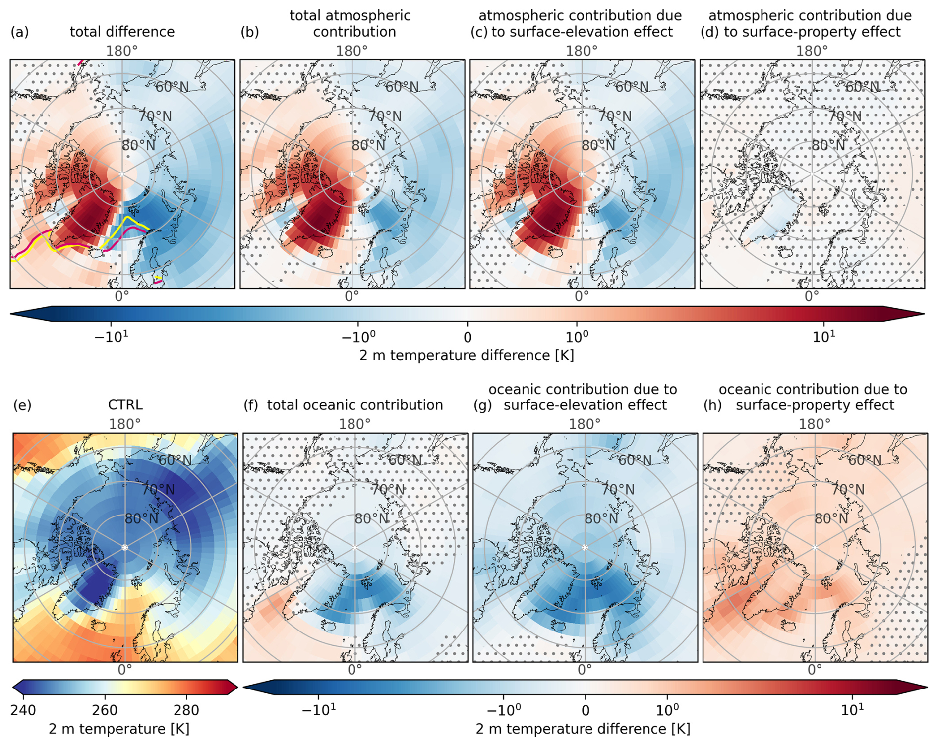
Figure 2 The 2 m air temperature in DJF. (a) The total difference (noGrIS − CTRL), (b) the total atmospheric contribution (noGrIS_atm − CTRL_atm), (c) the atmospheric contribution due to the GrIS surface-elevation effect (noGrIS_elev_atm − CTRL_atm), (d) the atmospheric contribution due to the GrIS surface-property effect (noGrIS_atm − noGrIS_elev_atm), (e) CTRL in absolute values, (f) the total oceanic contribution ((noGrIS − CTRL) − (noGrIS_atm − CTRL_atm)), (g) the oceanic contribution due to the GrIS surface-elevation effect ((noGrIS_elev − CTRL) − (noGrIS_elev_atm − CTRL_atm)) and (h) the oceanic contribution due to the GrIS surface-property effect (((noGrIS − CTRL) − (noGrIS_atm − CTRL_atm)) − ((noGrIS_elev − CTRL) − (noGrIS_elev_atm − CTRL_atm))). Stippling indicates regions that are not statistically significant at a significance level (α) exceeding 5 %, under the assumption of the null hypothesis that the distributions are equal. The yellow and magenta contour lines in panel (a) depict the March sea-ice extent in CTRL and noGrIS, respectively.

Summer

In summer, contributions over land and ocean are comparable, albeit weaker than in winter (Fig. 3). Differences include the absence of a dipole pattern in the atmosphere (Fig. 3b–d) and the emergence of a distinctly positive anomaly over Greenland (Fig. 3a). This anomaly is attributed to the impact of the GrIS surface-property effect on the atmosphere (Fig. 3d). The removal of the glacier mask and the absence of snow during summer allow surface temperatures in noGrIS to exceed the melting point. Additionally, darker surfaces are exposed in the absence of a snow cover. The ice-free ground and the more favorable climatic conditions promote the growth of grass and deciduous shrubs, specifically in the northeast of Greenland. This renders Greenland's vegetation similar to that found in the Siberian tundra. The vegetation further lowers the surface albedo in affected regions of Greenland, decreasing the surface albedo by up to 0.6 in noGrIS compared to CTRL. In contrast, CTRL maintains high surface-albedo values and surface temperatures limited to the melting point throughout the summer due to the prescribed ice sheet and its high surface elevation. In noGrIS, surface temperatures above freezing intensify radiative heating and alter the surface-energy budget. Additionally, surface roughness increases in noGrIS; however, a prior study suggests that this has a negligible impact on temperature anomalies compared to the changes in surface albedo (Stone and Lunt, 2013).

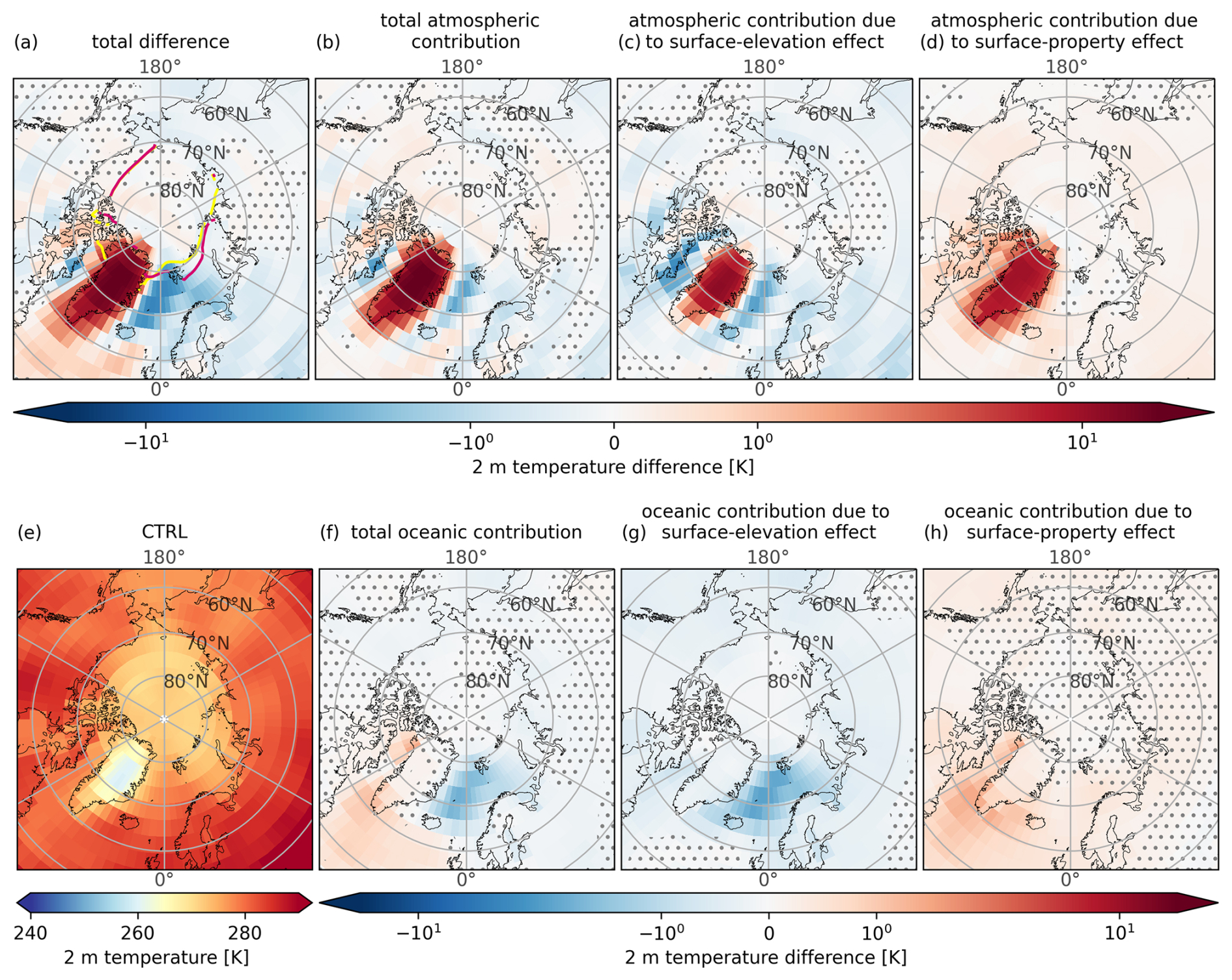
Figure 3 Similar to Fig. 2 but for JJA 2 m air temperature. The yellow and magenta contour lines in panel (a) depict the September sea-ice extent in CTRL and noGrIS, respectively. Note that the significance level in panel (d) is 10 %, and it is 5 % in all other panels.

Annual mean

Tallying up the positive and negative anomalies across the Northern Hemisphere, the net difference in the annual 2 m air temperature between noGrIS and CTRL approaches zero (−0.02 K, Fig. 4a). Removing the orography of the GrIS leads to a reduced global-mean sea-level pressure and a 0.3 K cooler Northern Hemispheric 2 m air temperature (Fig. 4c and g). This is evident from the sensitivity experiment noGrIS_elev, in which only the GrIS elevation effect has been considered. The interplay of altered GrIS surface properties, including surface temperatures rising above the melting point, the growth of vegetation, variations in radiative heating and surface roughness, exerts a counteractive warming effect (Fig. 4d and h).

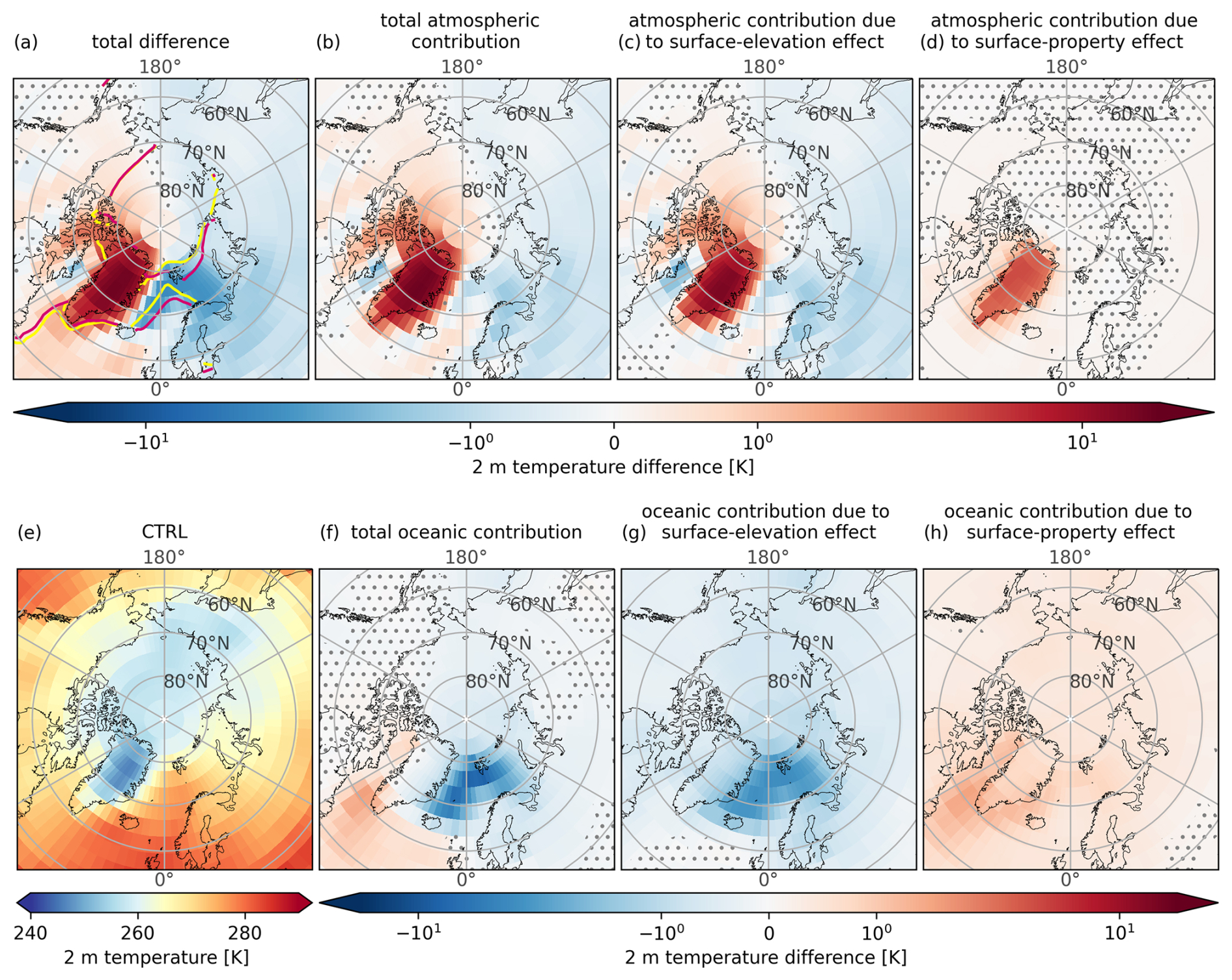
Figure 4 Similar to Fig. 2 but for the annual-mean 2 m air temperature. The yellow and magenta contour lines in panel (a) depict the March and September sea-ice extent in CTRL and noGrIS, respectively.

3.1.2 Dynamic response

Greenland Anticyclone and near-surface winds

In CTRL, the frigid conditions over Greenland create a favorable environment for the formation of a prominent high-pressure system, known as the Greenland Anticyclone (Hobbs, 1945) (Fig. 5a). On the other hand, a low-pressure system, referred to as Icelandic Low, resides in the route of dynamic cyclones over the warmer ocean around the tip of southeast Greenland and Iceland (Serreze et al., 1997).

In noGrIS, the lower orography and removed glacier mask, along with associated 2 m air warming, and the missing mechanical blocking result in a weaker Greenland Anticyclone (Fig. 5b) and a reinforced Icelandic Low (not shown). As a consequence, a notable difference in the strength and direction of annual 10 m winds over Greenland and its vicinity is visible in Fig. 5c. Being mostly driven by the mere GrIS height reduction, differences in 10 m winds are similar in noGrIS and noGrIS_elev (Fig. 5c and d). Around Greenland, annual-mean 10 m winds are weaker in the absence of the GrIS (Fig. 5c), decreasing the wind-stress curl on the ocean surface. Over the east coast of Greenland, the strength of the northeast winds decreases by up to 97 % (−5.7 m s⁻¹) and over the adjacent East Greenland Current by up to 80 % (−4.3 m s⁻¹). Over the Barents Sea and northern Scandinavia, winds are slightly stronger and adopt a more northerly trajectory (Fig. 5c). This facilitates the transport of cold polar air towards lower latitudes. The atmospheric impact becomes evident in the sensitivity experiments with a nudged ocean (noGrIS_atm). The cooling is strongest in winter, when the 2 m air temperature difference reaches up to −2.6 K in the Nordic Seas (Fig. 2b). The stronger and more northerly 10 m winds over the Nordic Seas change the wind stress on the surface and lead to a more southward drift of sea ice. This results in an expanded sea-ice cover in noGrIS relative to CTRL (Fig. 4a, further investigated in Sect. 3.2.1), which is amplified by the atmospheric cooling (Fig. 4b). The larger sea-ice extent reduces the heat loss of the ocean and enhances the cooling of the overlying atmosphere. Hence, when accounting for the oceanic feedback, the 2 m air temperature experiences a considerably stronger decrease over the Nordic Seas compared to the simulation with a nudged ocean (noGrIS_atm). This adds up to a total difference of up to −3.3 K in noGrIS relative to CTRL in the annual mean (Fig. 4a) and −6.0 K in winter (Fig. 2a). The sea ice also expands in other regions of the Northern Hemisphere, resulting in an overall negative temperature response of the ocean (Fig. 4f).

In noGrIS, 10 m winds also take a stronger easterly direction over Greenland as compared to CTRL (Fig. 5a and b). Originating from a warmer Greenland (Fig. 4a), when traversing the Baffin Bay towards the Canadian Arctic, they raise 2 m temperatures, heat the surface ocean and contribute to an intensified sea-ice melt in the western Arctic (Fig. 4a and Sect. 3.2). This is particularly pronounced in the Labrador Sea in summer, owing to the added warming due to the removed glacier mask (Fig. 3d). The heat absorbed in summer keeps Labrador Sea temperatures warmer throughout the entire year in noGrIS (Fig. 4f), as compared to the experiment considering only a lower surface elevation (noGrIS_elev, Fig. 4g). Hence, sea-ice formation is reduced in fall and winter in noGrIS (Fig. 2a). The resulting lower sea-ice cover allows for even more heat to be stored in the Labrador Sea in summer. In winter, the reduced sea-ice cover decreases the insulation of the ocean, leading to stronger heat loss of the ocean that further amplifies the atmospheric warming (Fig. 2h). Without considering the warming contribution due to the altered surface properties over Greenland, the 2 m air temperature over Greenland would be colder by up to 2.1 K (noGrIS_elev − noGrIS). The warming effect of altered Greenland surface properties is strongest in the Labrador Sea yet extends beyond this region (Fig. 4h), counteracting some of the ocean cooling effect associated with the lower GrIS surface elevation (Fig. 4g).

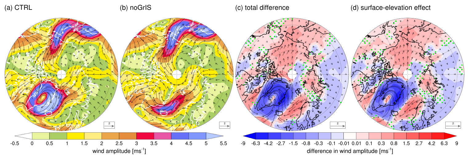
Figure 5 (a, b) Annual 10 m wind amplitude (contours) and direction (vectors, m s⁻¹). (c, d) Total difference (noGrIS − CTRL) and surface-elevation effect contribution (noGrIS_elev − CTRL) to the difference in the 10 m wind amplitude. Stippling designates statistically non-significant regions (see Fig. 2). Please note the logarithmic scale in panels (c) and (d).

Quasi-static wave

In the absence of the blocking GrIS topography, the quasi-static wave at 500 hPa is shifted northeastward over Greenland, while the dominant atmospheric wave number remains unchanged (Fig. 6). This shift results in a stronger meridional flow pattern, characterized by an enhanced southerly wind direction over Greenland and a more northerly wind direction over the Nordic Seas (Fig. 6b). This amplifies the influx of cold polar air towards the Nordic Seas and northern Scandinavia. As air masses are able to penetrate further into the interior of Greenland, they transform the circulation from a “flow around” into a more quasi-geostrophic “flow over” circulation, following Hakuba et al. (2012). The difference in the quasi-static wave is caused by the orographic effect, as suggested by similar patterns in noGrIS and noGrIS_elev (Fig. 6c and d). The GrIS surface-property effect slightly counteracts the normalized geopotential height reduction over Greenland, as depicted by the slightly less negative anomaly in Fig. 6c than in Fig. 6d.

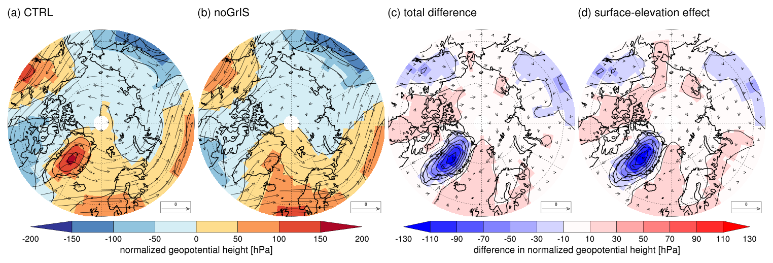
Figure 6 (a, b) DJF normalized geopotential height (contours) and flow direction (vectors, m s⁻¹) at 500 hPa. (c, d) Total difference (noGrIS − CTRL) and surface-elevation effect contribution (noGrIS_elev − CTRL) to the difference in the normalized geopotential height and flow direction at 500 hPa. Note that the entire region shown is statistically significant at α=5 %.

Storm tracks and precipitation

Differences in the large-scale circulation patterns also affect the trajectory of winter storm tracks in the Northern Hemisphere. In CTRL, the storms approaching Greenland, as they move from North America to Europe, are diverted south due to the high orography of the GrIS. Hence, storms pass Greenland mainly on its southern edge (Fig. 7a). Additionally, the pressure gradient between the Icelandic Low and the Greenland Anticyclone induces strong easterly onshore winds in southeast Greenland (Fig. 5a), which are associated with high amounts of precipitation. This is in line with Ohmura and Reeh (1991). Both of these dynamic effects contribute to orographic precipitation on the windward side of the mountains and explain the precipitation peak to the east of southern Greenland and over the south and southeast of Greenland (Fig. 8a). Characterized by the highest elevation and the coldest air temperatures, the interior of Greenland encounters mostly dry conditions.

In absence of the blocking GrIS, storms penetrate deeper into central Greenland in noGrIS (Fig. 7b–d). As more storms pass over Greenland in noGrIS, cyclonic activity decreases in the west of Greenland, specifically over the Canadian Arctic Archipelago, Baffin Bay and parts of Canada. The shifted quasi-static wave pattern and storm tracks redistribute the annual regional precipitation more homogeneously across Greenland (Fig. 8b–d). Precipitation decreases in the south and southeast of Greenland and increases in the northeast, where the air masses are forced to lift along the remaining orography. These changes in precipitation allow for less river discharge off the south coast of Greenland but more discharge off the east coast. The stronger storm activity over Greenland contributes to the aforementioned weaker Greenland Anticyclone and the deeper Icelandic Low.

Cyclonic activity increases slightly in the lee of Greenland. The higher frequency of storms to the southeast of Greenland increases precipitation over the adjacent ocean. It also explains some of the warmer 2 m air temperatures in this region in noGrIS (Fig. 2b), as storms usually carry not only moist but also warm air masses. In the Nordic Seas, this warming and cyclonic effect is overcompensated by the intensified inflow of polar air, advecting colder and drier air masses, while reducing the inflow of warm and moist Atlantic air. The similarity of the change pattern in the cyclonic activity and precipitation over Greenland and east of Greenland suggests that the main contribution stems from the lower GrIS elevation.

Figure 7 (a, b) Standard deviation (SD) of the DJF 2 to 5 d band-pass-filtered sea-level pressure (SLP) as a measure of cyclonic storm activity similar to Dethloff et al. (2004). (c, d) Total difference (noGrIS − CTRL) and surface-elevation effect contribution (noGrIS_elev − CTRL) to the differences in storm activity. Stippling designates statistically non-significant regions (α>10 %).

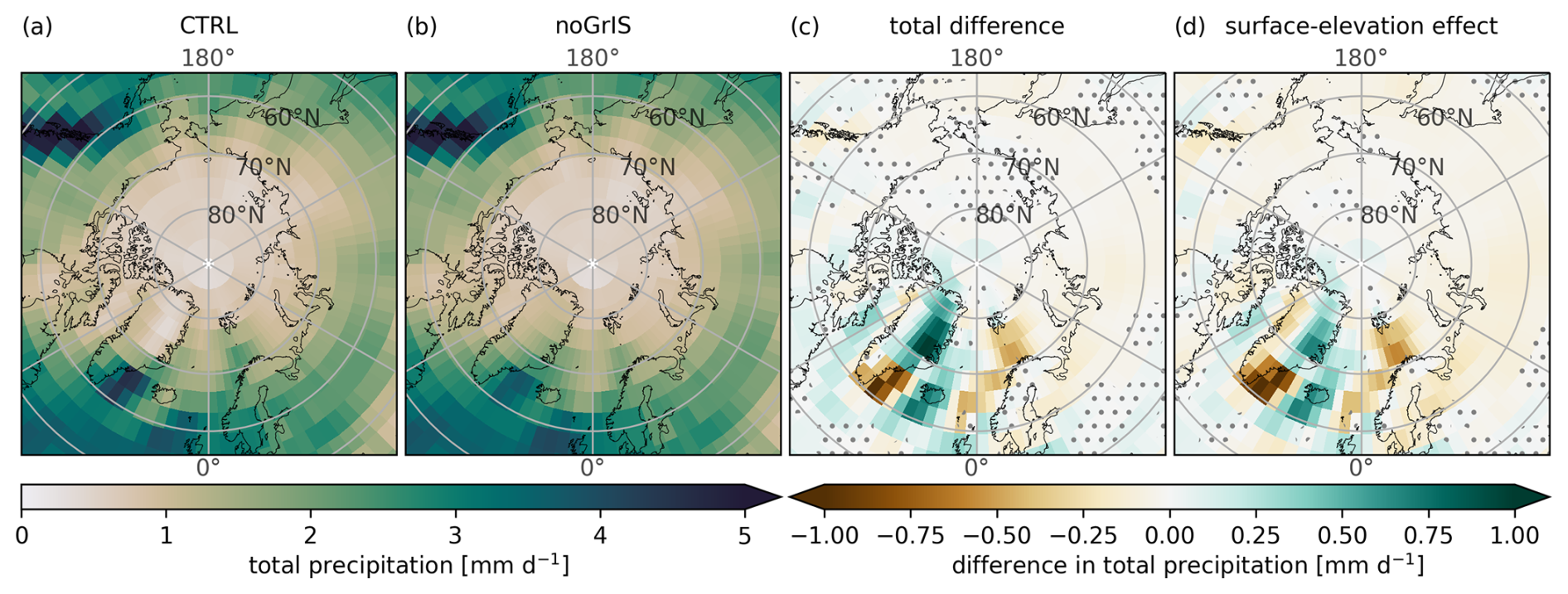
Figure 8 (a, b) Annual-mean total precipitation. (c, d) Total difference (noGrIS − CTRL) and surface-elevation effect contribution (noGrIS_elev − CTRL) to the differences in precipitation. Stippling designates statistically non-significant regions (see Fig. 2).

3.1.3 Drivers of the Greenland warming

To investigate the drivers of the strong warming across Greenland, we isolated the atmospheric and oceanic impact by calculating individual contributions from the sensitivity experiments (Fig. 9). Throughout all seasons, the temperature difference across Greenland is dominated by the atmospheric contribution. In winter, a strong warming relative to CTRL originates from the lower elevation of 1320 m of the GrIS (+9.6 K), encompassing two distinct effects. The first is the lapse-rate effect, which accounts for the rise in 2 m air temperature due to the lower GrIS surface elevation. The second is an atmospheric-circulation effect, such as the prevalence of more southerly high-altitude winds over Greenland and the increase in storm activity (Sect. 3.1.2). Altered GrIS surface properties only have an impact on the atmosphere in summer, when the surface is ice-free and snow-free (+7.1 K). The overall ocean contribution is slightly negative. While additional heat is stored in the ocean due to the warming of Greenland in response to the GrIS surface-property changes, the warming is offset by cooling driven by the reduced surface elevation (Figs. 2 and 3, Sect. 3.1.2). In the annual mean, the 2 m temperature over Greenland warms by 10.7 K.

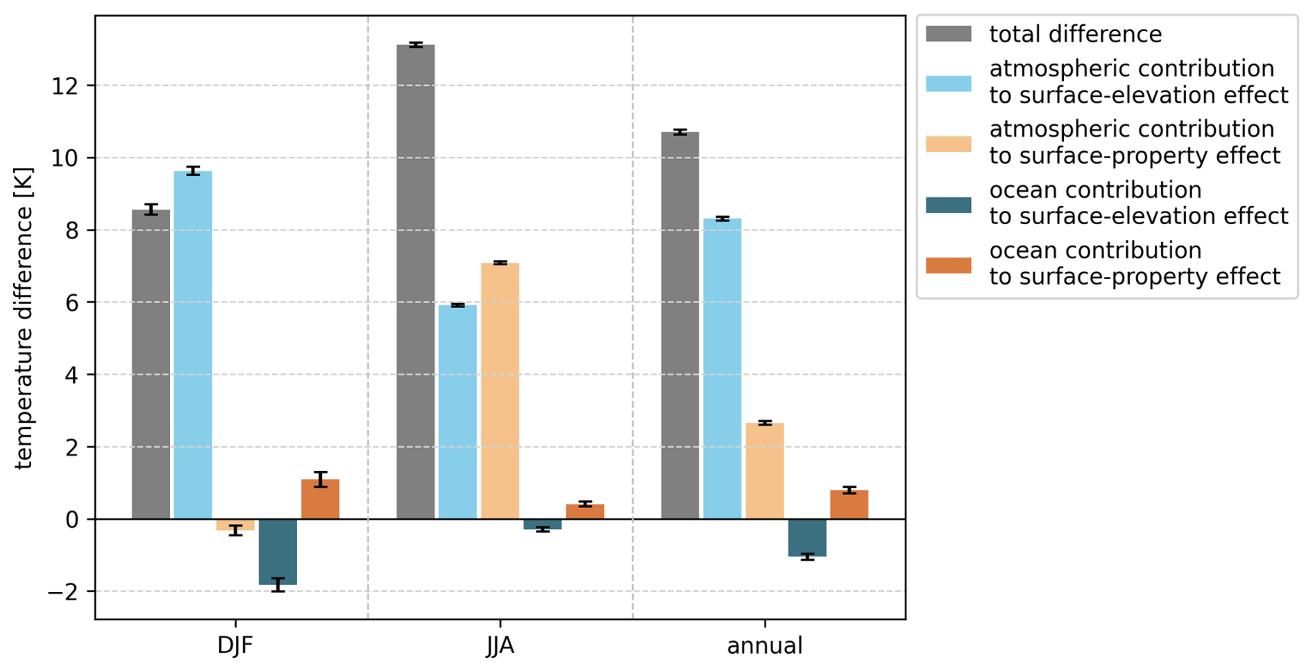
Figure 9 Atmospheric and oceanic contributions to the total 2 m air temperature difference (gray) averaged over Greenland in DJF, JJA and annually due to the altered GrIS surface elevation (blue) and properties (orange). Gray bars illustrate the total difference (noGrIS − CTRL). Light blue bars show the atmospheric contribution due to the lower surface elevation (noGrIS_elev_atm − CTRL_atm). Light orange bars depict additional atmospheric effects arising from the altered GrIS surface properties (noGrIS_atm − noGrIS_elev_atm). Dark blue bars represent the oceanic contribution due to the lower surface elevation ((noGrIS_elev − CTRL) − (noGrIS_elev_atm − CTRL_atm)). Dark orange bars depict the oceanic contribution due to the altered surface properties (((noGrIS − CTRL) − (noGrIS_atm − CTRL_atm)) − ((noGrIS_elev − CTRL) − (noGrIS_elev_atm − CTRL_atm))). Black whiskers designate the 90 % confidence interval.

3.2 Ocean response and feedback

The preceding analysis indicates that the GrIS substantially impacts the atmosphere through dynamical and thermodynamical processes. Differences in the 2 m air temperature, precipitation and wind stress across the Arctic and sub-Arctic region between CTRL and noGrIS directly influence the SST pattern, affect the spatial distribution of freshwater and contribute to buoyancy changes. In view of these direct connections, we investigate the impact of a disintegrated GrIS on the ocean in the subsequent sections. As the rate of ocean-mass exchange through the Arctic gateways affects the characteristics of both the Arctic Ocean and adjacent seas, we analyze differences in the transport of sea ice and water through the Arctic gateways between CTRL and the experiments with a disintegrated GrIS and summarize them in Table 2.

3.2.1 Ocean circulation changes

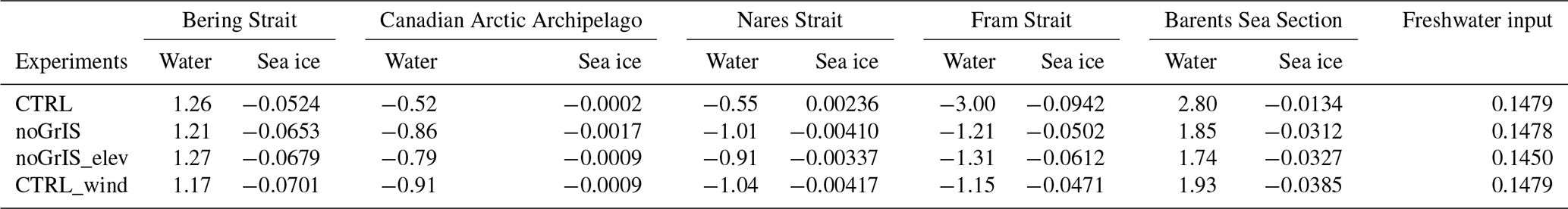
In noGrIS, the anticyclonic Beaufort Gyre is stronger and more extensive than in CTRL (Fig. 10a–d), and its core is slightly shifted towards the southeast (Fig. 10f and j). In the eastern Arctic, this changed circulation pattern favors the advection of freshwater from the Chukchi Sea along the coastline of Siberia towards the Laptev Sea, while reducing the influx of saline North Atlantic Ocean water into the Laptev Sea. The stronger Beaufort Gyre more effectively transports runoff from the Eurasian rivers away from their deltas into the Arctic Ocean. This is evident from the altered flow direction vectors and the freshening north of Eurasia, depicted in Fig. 10i–l. As a consequence, eastern Arctic waters are fresher throughout the entire water column in noGrIS than in CTRL (shown for the upper 100 m in Fig. 10k). In the western Arctic Ocean, the cyclonic coastal current, which originates from the Bering Strait and flows along the Canadian Arctic Archipelago towards Lincoln Sea, is weaker in noGrIS (Fig. 10b and j). Therefore, less freshwater is advected towards Ellesmere Island in noGrIS – visible in the positive salinity anomaly close to the northeastern Canadian Arctic Archipelago and off the northern coast of Greenland (Fig. 10i–l). The shift in the Beaufort Gyre leads to a twofold export of sea ice through the Barents Sea Section and a concurrent decrease in sea-ice export through Fram Strait by about 50 % in noGrIS compared to CTRL (Table 2). Further, the stronger northerly wind direction over the Barents Sea leads to a higher export of sea ice through the Barents Sea Section and to an atmospheric cooling (Sect. 3.1.2 and Fig. 2b). This results in a southward expansion of sea ice (Fig. 10g) and a cooling of the upper ocean until around 150 m depth (Fig. 11). The expanded sea-ice cover negatively feeds back onto the 2 m air temperature (Fig. 2f). As the sea-ice edge is located further south, sea ice melts further south in noGrIS, which leads to freshwater input into more southerly regions of the Nordic Seas.

The altered ocean currents due to the changed wind stress, however, are the primary driver of the freshening in the Nordic Seas (Fig. 10k and l). Alterations in the wind-stress curl on the upper Greenland and Norwegian Sea attenuate the local wind-driven ocean circulation, as evident by a weaker Greenland Sea Gyre (Fig. 10d). As a consequence, the influx of North Atlantic waters into the Nordic Seas via the Iceland–Scotland section is decreased, reducing the salt content of the Nordic Seas. The reduced northward transport of water by the Norwegian Atlantic Current through the Barents Sea Section (−33 %) also contributes to the freshening of the Arctic Ocean in noGrIS relative to CTRL. As a consequence, water exported through the eastern Fram Strait is fresher, amplifying the freshening of the Nordic Seas. This freshening is further intensified by enhanced runoff from northeast Greenland, caused by the precipitation changes (Sect. 3.1.2). Weaker wind stress along Greenland's east coast in noGrIS (Sect. 3.1.2) also reduces the export of water mass through the Fram Strait by about 60 %. Additionally, the changed wind stress leads to an eastward expansion of the East Greenland Current into the Nordic Seas, progressively mixing fresh and cold polar waters with North Atlantic water (Fig. 10i–l). This contributes to the freshening and cooling of the Nordic Seas. The East Greenland Current is also shallower in noGrIS compared to CTRL, leading to a positive temperature and salinity anomaly close to the shelf region at around 150 m depth. This change in the shelf region opposes the freshening and cooling in the central Nordic Seas until 150 m depth.

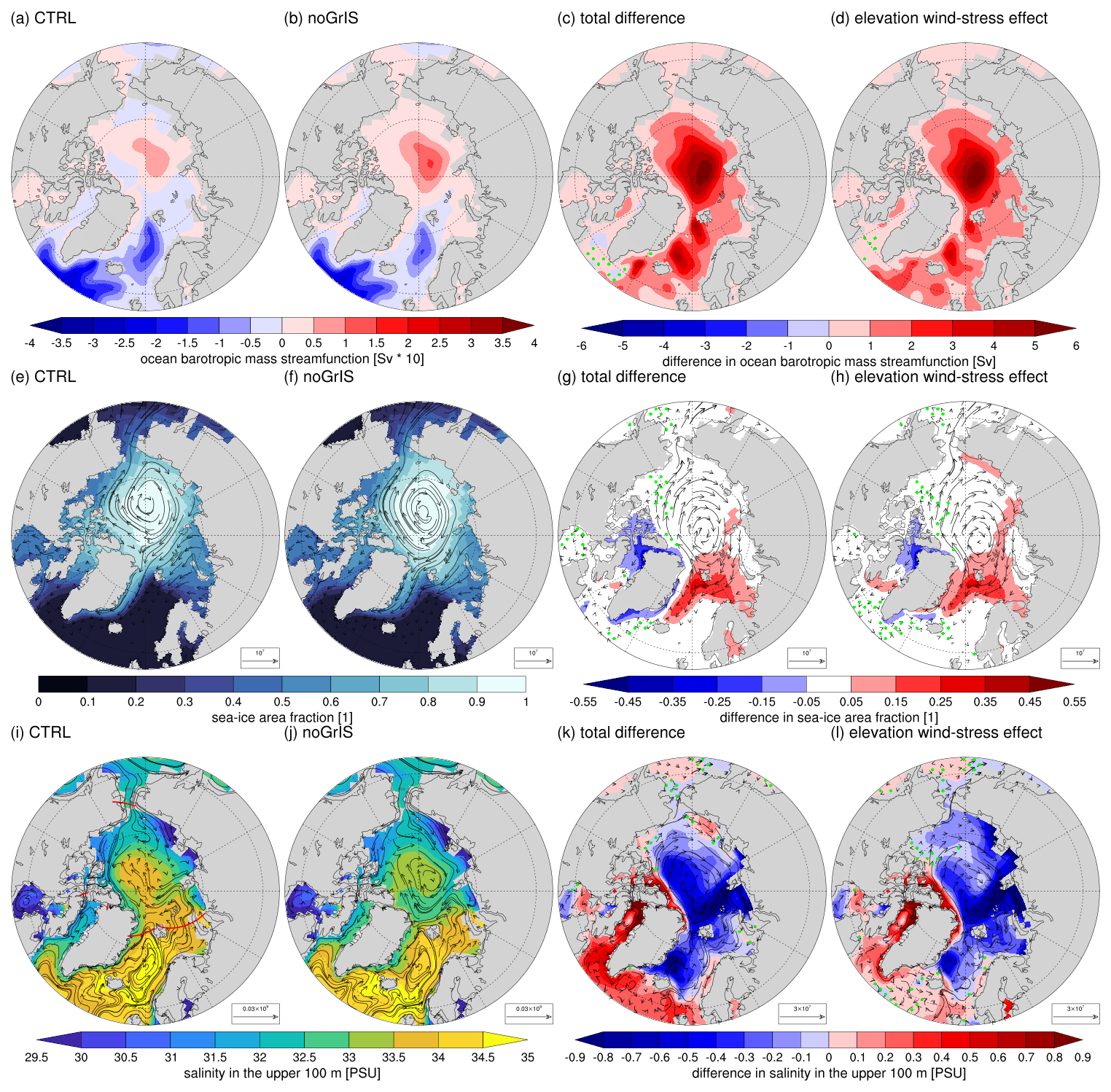
Figure 10 (a–d) Annual-mean ocean barotropic mass streamfunction, (e–h) annual-mean sea-ice fraction (contours) overlaid with sea-ice transports (vectors, kg s⁻¹) and (i–l) annual-mean salinity averaged over the upper 100 m (contours) overlaid with water-mass transports (vectors, kg s⁻¹). The two left columns show CTRL and noGrIS; the two right columns show the total difference (noGrIS − CTRL) and the wind-stress effect due to the lower GrIS surface elevation (CTRL_wind − CTRL). Stippling designates statistically non-significant regions (see Fig. 2). The red lines in panel (i) depict the locations of the transects used for the transport rates in Table 2.

The differences in Arctic Ocean circulation and a stronger sea-level gradient from the southeastern Arctic Ocean to the northern Baffin Bay in noGrIS (not shown) also induce differences in the mass transport through other ocean straits. The reduced ocean-mass export from the Arctic through the Fram Strait is balanced by higher ocean-mass export via western Arctic straits in noGrIS. Compared to CTRL, the Arctic water-mass export through Nares Strait doubles, and the transport through the Canadian Arctic Archipelago increases by 70 %. As the cyclonic rim current north of the Canadian Arctic Archipelago weakens, the exported water increasingly comprises saline water from off the northwest coast of Greenland and off the Canadian Arctic Archipelago rather than fresher Beaufort Sea water as in CTRL. The higher rate of sea-ice formation along the eastern edge of the Canadian Arctic Archipelago and the northern Baffin Bay in noGrIS_elev further adds to the higher salinity through brine rejection, as the sea ice is transported southward directly after its formation (Fig. 10f). Additionally, less freshwater is imported into the Baffin Bay by the West Greenland Current, nourished by fresh and cold water from the East Greenland Current. This makes the water in the Baffin Bay not only saltier (Fig. 10k) but also warmer than in CTRL. Another contribution to the salinity increase in the Baffin Bay in noGrIS is the slightly lower runoff into Baffin Bay due to higher evaporation over western Greenland (not shown). The resulting positive salinity anomaly across Baffin Bay extends to a depth of approximately 200 m, as the strait in the Canadian Arctic Archipelago and Nares Strait both have depths of less than 200 m.

Figure 11 Seawater potential density, salinity and in situ temperature in noGrIS (orange), noGrIS_elev (blue) and CTRL_wind (green) compared to CTRL (black) spatially averaged in the region of highest convection in the Nordic Seas (hatched line) and the Labrador Sea (solid line) in March. The regions used to calculate the vertical means are defined in Appendix A1.

Ocean currents transport the saltier water from the Baffin Bay southward through Davis Strait into the Labrador Sea. In the Labrador Sea, salinity and temperature are higher throughout the entire vertical column in absence of the GrIS (Fig. 11). The major driver of this change is the stronger advection of saline and warm water from the North Atlantic: in response to the altered wind stress, the eastern subpolar gyre circulation is weaker (Fig. 10d), reducing the northward transport of saline and warm water through the Iceland–Scotland section. A greater portion of the saline North Atlantic water remains within the subpolar gyre, where it moves westward towards the Labrador Sea. Another driver of the increase in temperature and salinity in the Labrador Sea is the reduced export of fresh and cold polar waters from the Arctic by the East Greenland Current through the Denmark Strait. This water is also warmer and more saline, as the subsurface water is delimited from the overlying fresh surface water and, hence, more closely aligns with the inflow characteristics of North Atlantic water. Lastly, the additional heat stored in the upper Labrador Sea, in response to the Greenland warming due to removing the glacier mask, results in the downward-transported water being relatively less cold than in CTRL.

The changes in the ocean circulation are mostly a consequence of the altered wind stress in response to the lower GrIS elevation. The modified GrIS surface properties only exert an amplifying influence, for example, on the strengthening of the Beaufort Gyre (Fig. 10b, f and j). Differences between the wind-stress sensitivity experiment (CTRL_wind) and the full elevation experiment (noGrIS_elev) indicate that atmospheric-circulation changes, following the lower GrIS elevation, compensate for some of the wind-stress-induced changes (e.g., changed transports through Fram Strait as shown in Table 2).

Table 2 Water and sea-ice transport rates into the Arctic Ocean through the five Arctic straits connecting the Arctic Ocean and the surrounding oceans. The Barents Sea Section is defined as the strait between Svalbard and Novaya Zemlya.

3.2.2 Deep-water formation changes

In the Nordic Seas, surface freshening (up to −1.4 psu) leads to the formation of a stronger pycnocline in noGrIS as compared to CTRL (Fig. 11). This manifests in less deep-water formation within the Nordic Seas in noGrIS. The stronger stratification results in less heat loss of the intermediate and deep ocean to the atmosphere. This warming in the ocean is particularly pronounced when also altering GrIS surface properties, as their warming effect on the Northern Hemisphere ocean strengthens the stratification. The reduction in deep-water formation further contributes to the weakening of the Greenland Sea Gyre (Fig. 10c).

The lower density in the Nordic Seas reduces the amount and density of overflow into the Denmark Strait (−1.3 Sv). This is partly driven by the lower GrIS elevation but dominated by the impact of altered GrIS surface properties, as they considerably contribute to the temperature increase and associated density decrease. The decrease in Denmark Strait overflow supplied from the Nordic Seas elevates the likelihood of deep convection in the Labrador Sea, which is the second key region for Northern Hemisphere deep-water formation in our model.

In the Labrador Sea, density increase in the subsurface 300 m, due to the enhanced inflow of salty waters, and density decrease below 400 m, due to persistent warming, weaken the pycnocline (Figs. 11 and 13a and b). This decreases vertical stability and intensifies intermediate and deep convection, which increases the average annual maximum regional mixed-layer depth to 2500 m in noGrIS compared to 1600 m in CTRL (Fig. 12). Stronger mixing with the underlying more saline and warmer layers amplifies the positive anomaly in upper-ocean salinity and temperature and thereby the buoyancy loss. While the local mixed-layer depth increases also in the Irminger Sea in noGrIS, this increase in the Labrador and Irminger Sea is insufficient to fully compensate for the reduced deep water from the Denmark Strait overflow and associated reduction in density at depth. This is visible in a slight decrease in North Atlantic Deep Water (NADW) density below 400 m in the Labrador Sea (Figs. 11 and 13a and b). The reduced density in NADW allows Antarctic Bottom Water (AABW) to expand upwards, leading to an upward shift of the transition between NADW and AABW at around 60° N at levels below 2500 m (Fig. 13c and d).

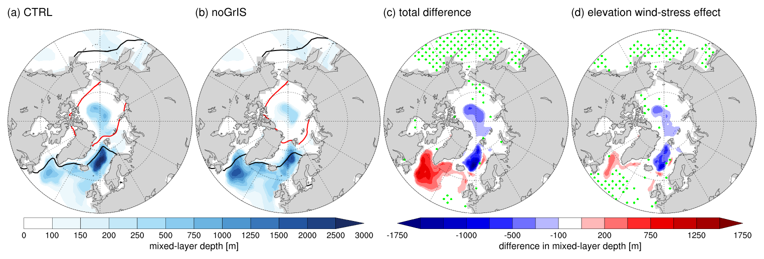
Figure 12 (a, b) Mixed-layer depth in the North Atlantic. (c, d) The total difference (noGrIS − CTRL) and the wind-stress effect due to the lower GrIS surface elevation (CTRL_wind − CTRL). For each grid cell the annual maximum value is shown. Stippling designates statistically non-significant regions (see Fig. 2). The red outline shows the minimum sea-ice extent in September and the black line the maximum extent in March. The regions chosen for the computation of the mixed-layer depth are shown in Appendix A1.

Deep-water formation in the Nordic Seas is reduced and relocated to the south, while being only partially compensated by enhanced deep-water formation in the Labrador Sea. For these reasons, the AMOC weakens at around 75° N and extends less far north at 60–65° N, while the maximum AMOC strength and depth in the subtropics remain almost unchanged (Fig. 13e and f). Additionally, the lower boundary of the AMOC shifts to shallower depths. The shallowing of the AMOC cell is strongest between 40 and 60° N, with a maximum shallowing of approximately −230 m at around 58° N. Both the GrIS surface-elevation effect and surface-property effect drive the AMOC cell shallowing and retreat, though the surface-elevation effect dominates the changes. The shallowing is also reflected in the increase in AABW below the subpolar gyre (Fig. 13c and d). Similar to the maximum strength of the AMOC, the Atlantic heat transport between 20 and 50° N changes only marginally (<2 %).

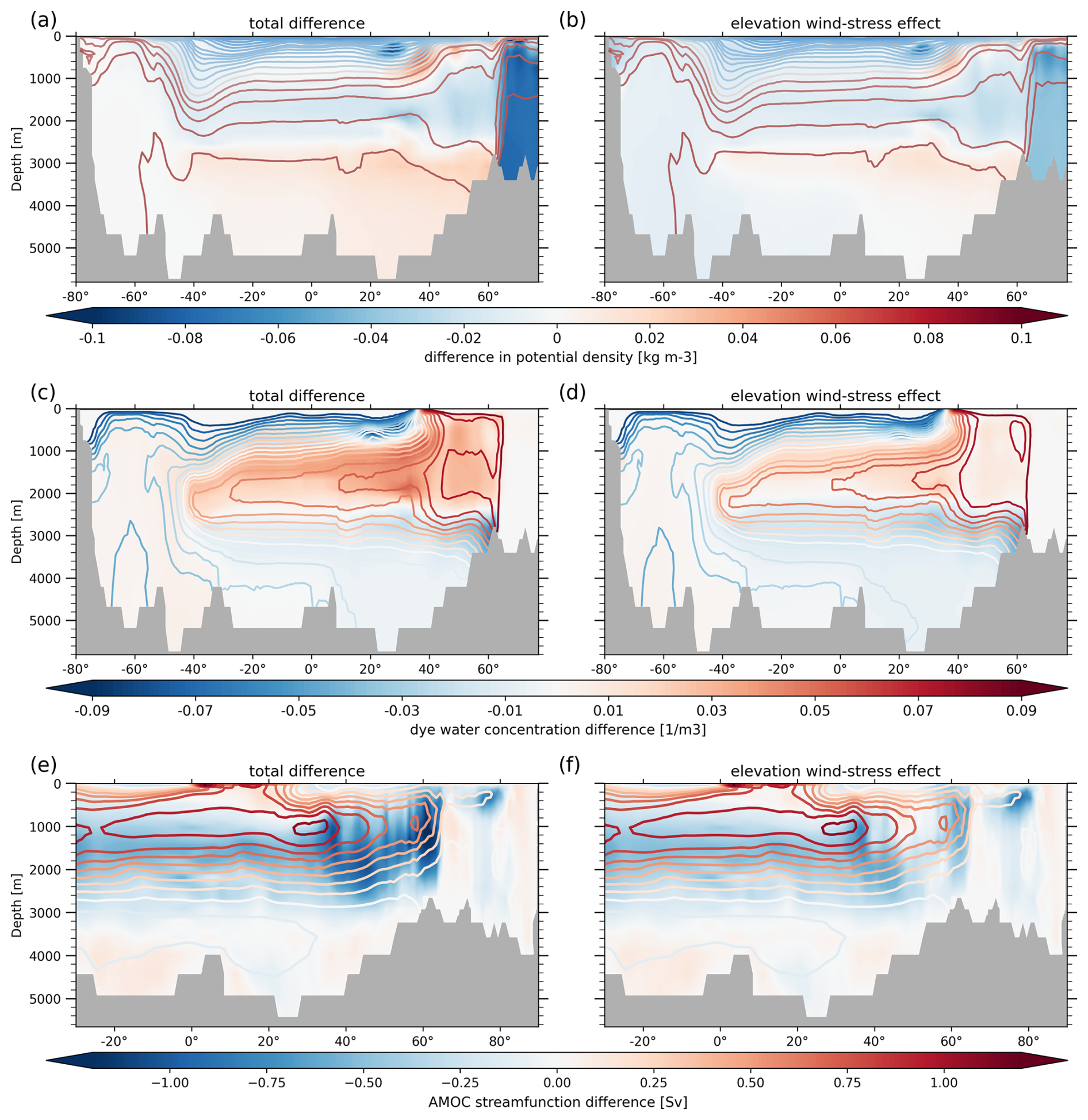
Figure 13 Cross-sections zonally averaged over the Atlantic Ocean. (a, b) Difference in potential density, (c, d) difference in dye water concentration as an indicator for the distribution of NADW and AABW, and (e, f) difference in the AMOC streamfunction. The differences are overlaid with the contour lines of CTRL. Please note a change in the intervals from 0.1 to 0.2 kg m⁻³ between the contour lines in panels (a) and (b) above and below 1026.4 kg m⁻³, respectively.

3.3 Remote changes

Climatic differences in response to the absence of the GrIS are not limited to the Northern Hemisphere (sub-)polar regions. On a larger scale, the dipole pattern of the 2 m air temperature difference in the Northern Hemisphere (Sect. 3.1.1) extends southward, causing a cooling over Europe. The cooling is strongest over Scandinavia, but it extends to parts of central Europe, reaching on average cooling of 1.2 K (noGrIS − CTRL, Fig. B1). Further, the difference in the atmospheric circulation causes a slight decrease in the storm activity over France, northwestern Germany and the United Kingdom but an increase over northern Scandinavia (Fig. B2).

In the subtropics, weaker zonal winds at around 40° N, in response to the reduced GrIS surface elevation and amplified by the altered GrIS surface properties, slightly shift the North Atlantic subtropical gyre southward (Fig. 13a and b). The displacement leads to an increase in the presence of subpolar water at lower latitudes, reflected in a negative salinity and temperature anomaly in the northern part of the subtropical gyre (not shown). Being slightly more dependent on temperature, the density increases in response to the cooling. Due to a contraction, the lower boundary of the North Atlantic subtropical gyre is shallower (Fig. 13a and b).

While the changes in the atmospheric circulation are substantial, we do not find statistically significant changes in atmospheric indices, such as the North Atlantic Oscillation (NAO), the Greenland Blocking Index (GBI) and the Northern Hemisphere jet stream position (not shown).

3.4 Disentangling the impact GrIS elevation and surface-property effect

The results presented in this paper show that a disintegration of the GrIS would have substantial implications for atmospheric and oceanic dynamics. Through our set of sensitivity experiments, we elucidate the distinct contributions of various factors involved in the complex interplay among the GrIS, atmosphere and the ocean, as illustrated by the schematic in Fig. 14.

CTRL and noGrIS differ in their Greenland surface elevation (Δ1320 m on average) and surface properties (i.e., removed glacier mask). The associated thermodynamic and dynamic changes in the atmosphere and the ocean are predominantly driven by the orographic effect. However, the altered surface properties of the GrIS play a significant role, primarily amplifying the climate response. Examples include the warming over Greenland or ocean-mass transport changes through the Canadian Arctic Archipelago. In a few instances, the altered GrIS surface properties have a counteractive effect, such as on the ocean-mass transport through the Bering Strait or the changes in the 500 hPa quasi-static wave. The main drivers of the ocean response vary also with depth. The elevation effect is important for the upper-ocean densities, while Greenland surface properties are controlling the intermediate and deep ocean response. The GrIS surface-property effect is particularly important in the Labrador Sea, where the ocean stores heat from excessive summer warming over Greenland, impacting ocean properties and dynamics, such as deep-water formation. Although most of the changes in response to a disintegrated GrIS are restricted to the surroundings of Greenland, we find a few changes in more remote areas, such as a cooling in central and northern Europe, a shallowing of the AMOC cell and a southward shift of the subtropical gyre, all dominated by the GrIS surface-elevation effect.

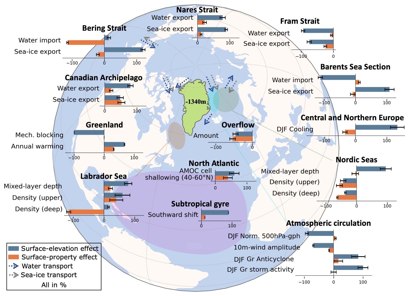
Figure 14 Contribution of the GrIS surface-elevation (blue) and the GrIS surface-property effect (orange) to the simulated climate changes in response to an absence of the GrIS, leading to a mean lower elevation of 1340 m and altered land cover (i.e., growth of grass and shrubs). The bars represent the respective contributions in percentages, while the whiskers illustrate the 90 % confidence intervals. If not stated differently, values are computed from annual-mean values, except for the contributions to the changes in the storm tracks, which are calculated from DJF hourly data, and the mixed-layer depth, which is computed from annual-maximum values. The elevation contributions are computed as (noGrIS − CTRL) $/$ (noGrIS_elev − CTRL) and the surface-property contribution as (noGrIS − CTRL) $/$ ((noGrIS − CTRL) − noGrIS_elev). Gray arrows show the direction of sea-ice transport and the blue arrows the direction of water-mass transport. The regions used to calculate the contributions are defined in Appendix A1. Gr: Greenland.

4 Discussion

Our use of a coupled atmosphere–ocean model with interactive vegetation and a sufficiently long model spin-up to reach equilibrium allowed us to generate a systematic set of sensitivity experiments that enables us to comprehensively investigate the interactions of the GrIS with the full climate system, including the deep ocean. Hence, our study extends prior studies that employed either atmosphere-only (e.g., Dethloff et al., 2004; Hakuba et al., 2012; Junge et al., 2005; Petersen et al., 2004), simplified ocean models (e.g., Lunt et al., 2004) or coupled simulations yet to achieve full oceanic equilibrium (Davini et al., 2015; Stone and Lunt, 2013; Toniazzo et al., 2004). While these studies suppressed the ocean influence to the climate response to varying degrees, our study transcends by adding knowledge on the deep-ocean response. Through the variety of sensitivity studies, our research not only describes the changes but disentangles, attributes and quantifies the drivers of the ocean response.

For the atmospheric response, strong similarities to previous research findings exist. For example, the redistribution of precipitation, mainly as a consequence of the lower GrIS elevation as previously found (Stone and Lunt, 2013), emerges as a robust feature across various climate models (Davini et al., 2015; Dethloff et al., 2004; Lunt et al., 2004; Solgaard and Langen, 2012; Toniazzo et al., 2004; Petersen et al., 2004). Further, the strongest warming in response to a removal of the GrIS occurs consistently over Greenland in all models (Crowley and Baum, 1995; Davini et al., 2015; Dethloff et al., 2004; Hakuba et al., 2012; Junge et al., 2005; Lunt et al., 2004; Ridley et al., 2005; Toniazzo et al., 2004; Vizcaíno et al., 2008), with a highest positive anomaly in summer attributed to the altered GrIS surface properties (Davini et al., 2015; Lunt et al., 2004; Ridley et al., 2005; Solgaard and Langen, 2012; Stone and Lunt, 2013; Toniazzo et al., 2004). While the largest climate responses broadly align between various studies, owing to the dominance of the elevation effect, differences occur due to the utilized model systems (e.g., coupled atmosphere and ocean component) as well as the experimental setup (e.g., surface-albedo adjustments or isostatically adjusted vs. non-adjusted bedrock vs. surface elevation set to sea level). In winter, the lapse-rate effect dominates differences in temperatures over Greenland between noGrIS and CTRL, but our results also show that changes in the atmospheric circulation contribute to the winter temperature response. The latter supports findings by Stone and Lunt (2013) and Toniazzo et al. (2004) but is contrary to Lunt et al. (2004), who suggested that circulation changes are not decisive. We also find an increase in the cyclonic activity over Greenland, confirming previous findings (Vizcaíno et al., 2008; Hakuba et al., 2012; Junge et al., 2005). Together with the altered temperature, the increased cyclonic activity over Greenland leads to the weakening of the Greenland Anticyclone and a deepening and expansion of the Icelandic Low (Toniazzo et al., 2004; Petersen et al., 2004; Davini et al., 2015). Cyclonic activity also increases to the east of Greenland, which is consistent with findings by Petersen et al. (2004) and Dethloff et al. (2004) but contrasts findings by Junge et al. (2005), Hakuba et al. (2012), Lunt et al. (2004) and Vizcaíno et al. (2008). This indicates that the local response is predominantly similar and robust against different model systems, whereas the distant response relies more on the type of coupling and/or the usage of simple methods for the adjustment of the GrIS orography and surface properties as well as on the resolution, as suggested previously by Junge et al. (2005).

In our simulations, the removal of the GrIS leads to an eastward shift of the 500 hPa quasi-static wave over Greenland. Further, we find that the shifted 500 hPa quasi-static wave plays a pivotal role in shaping the temperature response in our simulations by intensifying the southerly wind component at 500 hPa over Greenland. The shift is accompanied by altered 10 m winds, resembling Toniazzo et al. (2004), which advect warm air from Greenland towards the Canadian Arctic Archipelago and the Labrador Sea. The change in winds results in a warming of the western Arctic. While this process is in line with Davini et al. (2015), it contrasts findings by Petersen et al. (2004) and Junge et al. (2005), who linked the warming to the west of Greenland to the reduced Greenland blocking, which allows for cold Arctic air that usually remains west of Greenland to disperse further eastward. However, their results were obtained with atmosphere-only models, unchanged GrIS surface properties and simple methods for the reduction of the GrIS elevation, neglecting important feedbacks between the ocean, topography and the orography. The shifted wave additionally induces an enhanced northerly inflow of cold polar air over the Barents Seas and Scandinavia, resulting in a local cooling, similar to Lunt et al. (2004). In addition to Lunt et al. (2004), who found that the atmospheric change also leads to near-surface cooling that triggers sea-ice expansion in the Barents Sea, our sensitivity studies suggest that a stronger northerly component in the wind stress intensifies the southward drift of sea ice. The associated sea-ice expansion creates a negative feedback loop that further cools the overlying atmosphere. This mechanism contrasts with prior findings that associated parts of the cooling over the Barents Sea and neighboring land areas with reduced heat advection due to a decreased storm activity (south-)east of Greenland (Lunt et al., 2004; Ridley et al., 2005; Stone and Lunt, 2013; Toniazzo et al., 2004; Vizcaíno et al., 2008).

Differences in AMOC strength can have substantial impacts on the Atlantic heat transport between lower and higher latitudes (Jackson et al., 2015; Liu et al., 2024). Davini et al. (2015) suggested a weakening of the AMOC associated with a reduced poleward Atlantic heat transport as an additional mechanism for the cooling over the North Atlantic and Eurasia. Their AMOC reduction is a consequence of reduced deep-water formation in the Nordic Seas and Labrador Sea. We also simulate reduced deep-water formation in the Nordic Seas, whereas the mixed-layer depth in the Labrador Sea increases. This can explain the difference in the AMOC response to an absent GrIS. In our simulations, the maximum AMOC strength as well as the Atlantic heat transport at the latitudes of central Europe remain nearly unchanged, but the NADW cell is shallower. Our sensitivity experiments demonstrate that this cooling also prevails in simulations in which the AMOC experiences only a marginal weakening. Similar to our results, Toniazzo et al. (2004) also did not find a significant difference in the AMOC strength following a removal of the GrIS. This suggests that the contribution of the AMOC may be smaller than indicated in Davini et al. (2015) and that changes in the AMOC may not be the primary driver of the cooling over Eurasia and the Nordic Seas. Our analysis reveals a reduced heat loss of the Nordic Seas due to the larger sea-ice cover. The additional sea ice insulates the ocean and leads to a stronger ocean stratification that prevents the heat loss of the inflowing subsurface Atlantic waters. As a consequence, the water exported from the Nordic Seas through the Denmark Strait is warmer and contributes to the subsurface warming in the subpolar gyre. The cooling over the Nordic Seas emerges as a consequence of the combined effects of the altered atmospheric circulation and the expanded sea-ice cover that reduces heat loss towards the atmosphere. Over most of Scandinavia, the cooling is dominated by atmospheric feedbacks (Fig. B1). South and east of Scandinavia the oceanic impact ceases.

Our study also shows that the disintegration of the GrIS has considerable implications for the ocean circulation and ocean properties in the Arctic and North Atlantic Ocean. For example, our findings underscore the crucial role of changes in the wind stress on the upper-ocean circulation, particularly the Nordic Seas, influencing the water-mass exchange with the Arctic Ocean, a finding which is in accordance with Davini et al. (2015). However, Davini et al. (2015) proposed that the GrIS elevation effect leads to the transport of fresher waters by the East Greenland Current along Cape Farewell toward the Labrador Sea. In their study, this process freshens the Labrador Sea, lowers convection and weakens the AMOC. While we also simulate fresher Nordic Seas, water in the Denmark Strait is fresher only until a depth of around 100 m but more saline and warmer in lower layers, due to the weaker (warmer and saltier) East Greenland Current. The anomaly extends across the Irminger Sea toward the Labrador Sea, where it contributes to the simulated warmer and more saline conditions. Although the increase in salinity, in the absence of the GrIS, leads to an increase in upper-ocean density in our study, deep convection does not increase enough to compensate for the reduced influx of Denmark Strait overflow. Hence, the NADW cell is shallower in noGrIS relative to CTRL. We also find that altered ocean dynamics in the western Arctic, regarded as negligibly influenced by the wind-stress changes in Davini et al. (2015), also contribute to the simulated changes in the Labrador Sea. The discrepancies between our study and Davini et al. (2015), specifically in the Labrador Sea, are likely related to differences in the model system and boundary conditions. Possible explanations include the usage of an isostatically adjusted bedrock in our study compared to a non-adjusted bedrock in Davini et al. (2015), though Toniazzo et al. (2004) showed only minor differences in their impacts. Alternatively, the weak drift in the model of Davini et al. (2015) may cause different results. These discrepancies highlight the complex and regionally specific responses of the atmosphere and ocean to the absence of the GrIS, emphasizing the need for further research and model comparisons to fully grasp the broader implications of the presented climatic changes.

5 Conclusions

The experiments in this study simulate the climate following a complete disintegration of the GrIS. Employing a coupled atmosphere–ocean model allowed us to provide a distinct attribution and quantification of the simulated global atmospheric and oceanic responses to their respective drivers. Our study unveils that the climatic response to a disintegrated GrIS is dominated by orographic effects and associated changes in the wind and wind stress, attributable to a reduced surface elevation of on average 1320 m. Hence, the primary impact of the GrIS is induced by the ice sheet acting as a mechanical barrier. While this finding is consistent with previous research (e.g., Petersen et al., 2004), our study extends this understanding by revealing that altered GrIS surface properties amplify the majority of the climatic changes while they counteract some of them – for example, the change in ocean-mass transport through the Barents Sea Section and the Bering Strait. For the first time, an analysis reveals that the GrIS surface-property effect exerts a dominant influence in certain regions, which is notably pronounced in the Labrador Sea. We discern that the contribution of the effects varies not only horizontally but also vertically within the ocean. While changes in the elevation yield the greatest influence in the upper-ocean layers, alterations in the surface properties emerge as an important driver of oceanic changes in intermediate and deep layers. This distinction is unveiled only due to the use of a coupled model system including a fully spun-up deep ocean. Further, our analysis reveals that the impact of the GrIS extends beyond the Northern Hemisphere (sub-)polar region. A removal of the GrIS causes a southward shift and shallowing of the North Atlantic subtropical gyre and a cooling of central and northern European 2 m air temperatures. Despite the physical impact described in the present study, it should also be noted that a potential disappearance of the GrIS under future global warming scenarios (Aschwanden et al., 2019) would have considerable socioeconomic consequences. To investigate whether the potential disappearance of the GrIS would be irreversible even under subsequently lowered greenhouse gas emissions, future work will use a comprehensive fully coupled ESM encompassing dynamic ice sheets and vegetation (see Mikolajewicz et al., 2024, for the model setup). This will allow us to unravel so-far-neglected feedbacks between ice sheets and the climate system, while addressing the uncertainties that are associated with disregarding ice-sheet dynamics in simulations of the future climate with a comprehensive ESM.

Our analysis underscores the importance of taking into account all interactions and feedbacks between the GrIS and the full climate system when studying the future climate. To achieve this, it is not only imperative to allow for interactions between the different model components but also to consider long timescales of more than 5000 years, allowing the deep ocean sufficient time to adjust to alterations in the Earth system. Our approach fills a critical gap, as the ocean response to a disintegrated GrIS had not previously been systematically linked to the surface-elevation and surface-property effect, despite playing a substantial role in driving climate dynamics. This advances our understanding of the interplay of the GrIS with the full climate system, including the deep ocean.

Appendix A: Regional means

Table A1 Regions used for the area means.

Appendix B: Climate response in remote areas

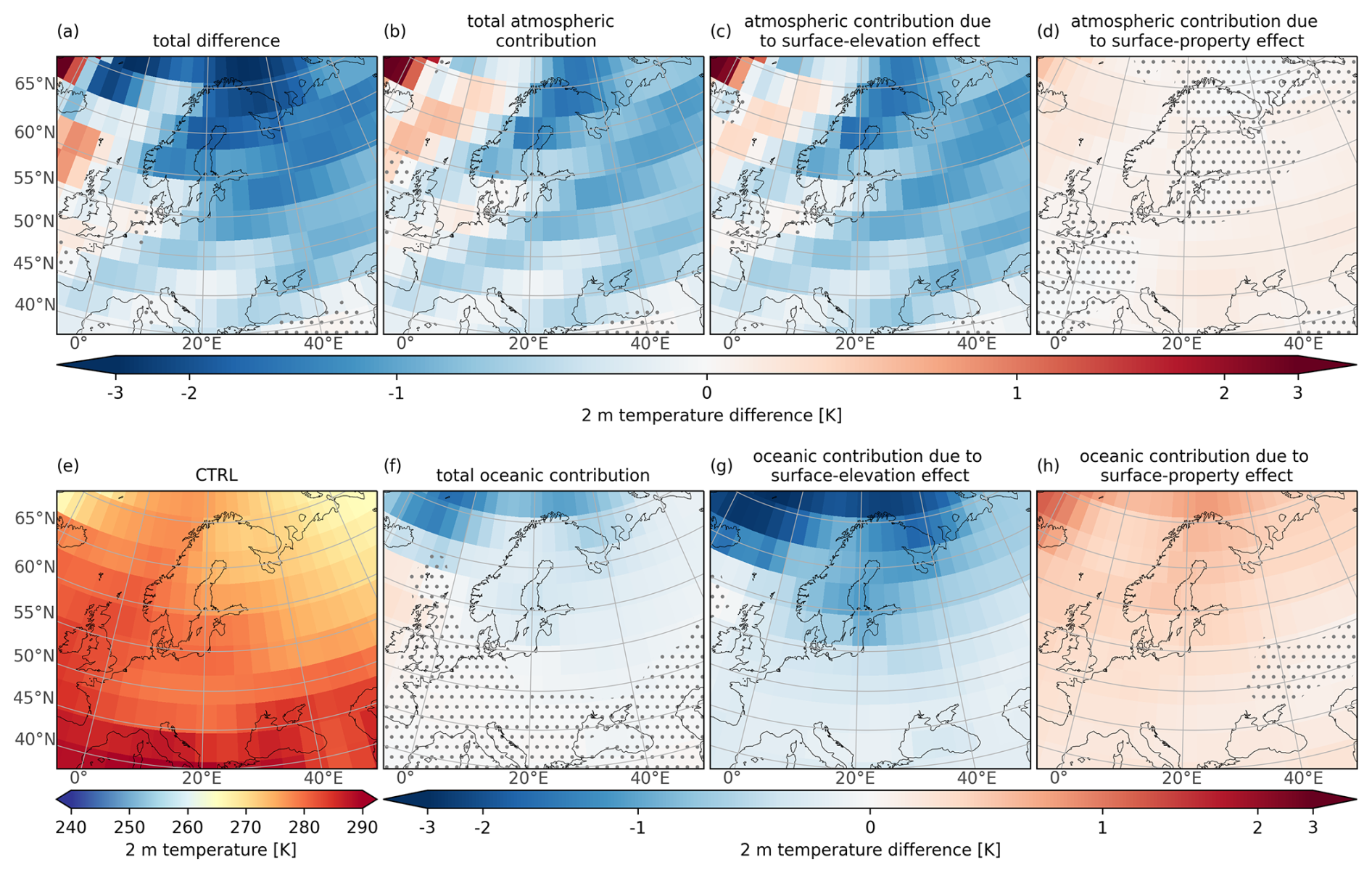
Figure B1 Annual-mean 2 m air temperature over northern and central Europe. (a) The total difference (noGrIS − CTRL), (b) the total atmospheric contribution (noGrIS_atm − CTRL_atm), (c) the atmospheric contribution due to the GrIS surface-elevation effect (noGrIS_elev_atm − CTRL_atm), (d) the atmospheric contribution due to the GrIS surface-property effect (noGrIS_atm − noGrIS_elev_atm), (e) CTRL in absolute values, (f) the total oceanic contribution ((noGrIS − CTRL) − (noGrIS_atm − CTRL_atm)), (g) the oceanic contribution due to the GrIS surface-elevation effect ((noGrIS_elev − CTRL) − (noGrIS_elev_atm − CTRL_atm)) and (h) the oceanic contribution due to the GrIS surface-property effect (((noGrIS − CTRL) − (noGrIS_atm − CTRL_atm)) − ((noGrIS_elev − CTRL) − (noGrIS_elev_atm − CTRL_atm))). Stippling designates statistically non-significant regions (see Fig. 2).

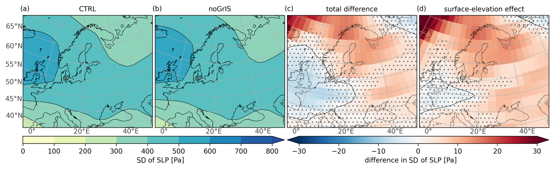
Figure B2 (a, b) Standard deviation (SD) of the DJF 2 to 5 d band-pass-filtered sea-level pressure (SLP) as a measure of cyclonic storm activity similar to Dethloff et al. (2004) over northern and central Europe. (c, d) Total difference (noGrIS − CTRL) and surface-elevation effect contribution (noGrIS_elev − CTRL) to the differences in storm activity. Stippling designates statistically non-significant regions (α>10 %).