Carbon cycle and climate feedbacks under CO₂ and non-CO₂ overshoot pathways

Reducing emissions of non-carbon dioxide (CO₂) greenhouse gases (GHGs), such as methane (CH₄) and nitrous oxide (N₂O), complements CO₂ mitigation in limiting global warming. However, estimating carbon–climate feedback for these gases remains fraught with uncertainties, especially under overshoot scenarios. This study investigates the impact of CO₂ and non-CO₂ gases with nearly equal levels of effective radiative forcing on the climate and carbon cycle, using the Earth system model (ESM) IPSL-CM6A-LR. We first present a method to recalibrate methane and nitrous oxide concentrations to align with published radiative forcings, ensuring accurate model performance. Next, we carry out a series of idealised ramp-up and ramp-down concentration-driven experiments and show that, while the impacts of increasing and decreasing CO₂ and non-CO₂ gases on the surface climate are nearly equivalent (when their radiative forcing magnitudes are set to be the same), regional differences emerge. We further explore the carbon cycle feedbacks and demonstrate that they differ under CO₂ and non-CO₂ forcing. CO₂ forcing leads to both carbon–climate and carbon–concentration feedbacks, whereas non-CO₂ gases give rise to the carbon–climate feedback only. We introduce a framework, building on previous studies that addressed CO₂ forcing, to separate the carbon–climate feedback into a temperature term and a temperature–CO₂ cross-term. Our findings reveal that these feedback terms are comparable in magnitude for the global ocean. This underscores the importance of considering both terms in carbon cycle feedback framework and climate change mitigation strategies.

1 Introduction

Increases in the atmospheric concentrations of carbon dioxide (CO₂), methane (CH₄), and nitrous oxide (N₂O) have predominantly caused human-induced climate change since the preindustrial period. They contributed nearly 63 %, 11 %, and 6 %, respectively, to the total effective radiative forcing (ERF) over the 1960–2019 period (Canadell et al., 2021). Anthropogenic CO₂ emissions are dominated by the combustion of fossil fuels (FFs) and land-use change (LUC), CH₄ emissions by FF and the agricultural sector, and N₂O emissions by the use of nitrogen fertiliser and manure. CH₄ and N₂O have atmospheric lifetimes of 11.8 ± 1.8 years and 109 ± 10 years and 100-year global warming potentials (GWP100) of 27.9 and 273, respectively (Forster et al., 2021; Myhre et al., 2013).

Mitigation of non-CO₂ greenhouse gases (GHGs) is an essential strategy to limit global warming in the context of the Paris Agreement's temperature target (Abernethy et al., 2021; Jones et al., 2018; Rao and Riahi, 2006; de Richter et al., 2017; Tanaka et al., 2021). The reduction in CH₄ emissions can lead to a rapid decrease in the radiative forcing and may limit the peak warming (Mengis and Matthews, 2020; Montzka et al., 2011). To facilitate the achievement of the Paris Agreement temperature target, the Global Methane Pledge was adopted to reduce anthropogenic CH₄ emissions by 30 % over the 2020–2030 period (CCAC, 2021). Several existing studies have confirmed the technical and socioeconomic capacities to reduce the global methane emissions and benefits for reducing atmospheric pollution (Höglund-Isaksson et al., 2020; Jackson et al., 2021; Malley et al., 2023; Nisbet et al., 2020). Atmospheric methane removal methods have also been discussed in some studies (Boucher and Folberth, 2010; Jackson et al., 2021; Mundra and Lockley, 2023), but they are still in their infancy.

Numerous studies have investigated the impacts of changes in the emissions/concentrations of CO₂ and non-CO₂ GHGs on the Earth system. The Precipitation Driver and Response Model Intercomparison Project (PDRMIP) focused on the role of different climate change drivers on the mean and extreme precipitation changes using a set of idealised perturbed experiments (Myhre et al., 2017). Richardson et al. (2019) revealed spatial and temporal differences in the surface temperature response to different forcings, such as CO₂ and CH₄, in part due to the physiological CO₂ warming over the densely vegetated regions that is absent under non-CO₂ forcing. This physiological warming occurs because plants close their stomata under elevated CO₂, reducing transpiration and decreasing latent heat loss, which causes a local surface warming. Nordling et al. (2021) further demonstrated that the change in long-wave clear-sky emissivity is the key driver of the differences in temperature response between GHG forcings. Using intermediate-complexity Earth system climate model simulations, Nzotungicimpaye et al. (2023) showed that delaying methane mitigation has implications both for meeting the stringent temperature targets and for the climate over many centuries. Using Earth system model (ESM) simulations, Tokarska et al. (2018) showed that non-CO₂ forcing reduces the remaining carbon budget due to its direct radiative effect on surface temperature, causing additional warming. Fu et al. (2020) showed that non-CO₂ GHGs, which have a shorter atmospheric lifetime than CO₂, may have long-term consequences on climate through their impacts on the carbon cycle, namely, warming from non-CO₂ GHGs weakening land and ocean carbon sinks.

The weakening of land and ocean carbon sinks due to non-CO₂ GHGs underscores the importance of understanding the differences in carbon cycle feedbacks between CO₂ and non-CO₂ GHGs. Only the changes in CO₂ concentrations give rise to the carbon–concentration feedback, which is the response of the land and ocean carbon uptake to the changes in CO₂ concentration, mainly via the stimulation of photosynthesis by the CO₂ fertilisation effect on land and the solubility pump in the ocean. The changes in both CO₂ and non-CO₂ concentrations lead to the carbon–climate feedback (γ), that is, the response of the land and ocean carbon uptake to climate change, mainly via the increased plant and soil respiration over land and reduction in the CO₂ solubility in the ocean with warming (Arora et al., 2013; Schwinger et al., 2014; Zickfeld et al., 2011). Under changing CO₂ concentrations, land and ocean carbon storages respond to both carbon–concentration and carbon–climate feedbacks. However, the interaction between these feedbacks can introduce a nonlinearity into the system, whereby the combined effect is not simply the sum of the individual feedbacks (Schwinger et al., 2014; Zickfeld et al., 2011). Thus, temperature-mediated feedback can differ under changing versus constant CO₂ levels, an important distinction when comparing CO₂ and non-CO₂ GHG feedback mechanisms. Here, it is also important to recognise that other factors, such as time lags and potential irreversibilities in the climate system, may also contribute to these differences (Boucher et al., 2012; Chimuka et al., 2023; Schwinger et al., 2014).

Previous studies investigated the nonlinearities in the carbon cycle feedback, showing that the cross-term – arising from interactions between changing atmospheric CO₂ and temperatures – can be comparable in size with γ (Schwinger et al., 2014; Zickfeld et al., 2011). They attributed the nonlinearity to the different responses of the land biosphere to the temperature changes, depending on the presence or absence of the CO₂ fertilisation effect, and to the weakening of ocean circulation and mixing between water masses of different temperatures. However, these studies did not consider non-CO₂ GHGs.

Previous studies have also examined the impact of declining atmospheric CO₂ concentration on the climate and carbon cycle (Boucher et al., 2012; Chimuka et al., 2023; Jones et al., 2016; Koven et al., 2023; Melnikova et al., 2021; Schwinger and Tjiputra, 2018). During the period of decreasing atmospheric CO₂ concentration and temperature (ramp-down), the β and γ feedbacks arise from both the reduction in CO₂ levels and temperature and the inertia of the carbon cycle – specifically, the altered land and ocean carbon pools resulting from prior increases in the CO₂ concentration and temperature (Chimuka et al., 2023; Zickfeld et al., 2016). Melnikova et al. (2021) showed that this leads to an amplification of the β and γ feedbacks under decreasing CO₂ concentration and temperature. The effectiveness of non-CO₂ mitigation has been explored and is an integral part of the integrated assessment models (Ou et al., 2021; Rao and Riahi, 2006; Tanaka et al., 2021). However, few studies have investigated the effects of declining non-CO₂ GHG concentrations on the climate and carbon cycle using Earth system models (ESMs). Abernethy et al. (2021) used an ESM to demonstrate the effectiveness of methane removal in reducing global mean surface temperature, complementing negative CO₂ emissions. Thus, the purpose of this study is 2-fold:

• to clarify whether the climate and carbon cycle responses to declining CO₂ and non-CO₂ GHGs differ globally and regionally,

• to investigate the nonlinearities of carbon cycle feedbacks under CO₂ and non-CO₂ GHG decrease and the implications for climate change mitigation.

Here, we conduct a series of idealised CO₂ and non-CO₂ (CH₄ and N₂O) concentration-driven ramp-up and ramp-down experiments using the IPSL-CM6A-LR ESM. We then compare the global and spatial impacts of CO₂ and non-CO₂ concentration changes on climate and the carbon cycle under overshoot pathways.

2 Data and methods

2.1 Recalibration of model's CH₄ and N₂O concentrations

We use Version 6 of the Institut Pierre-Simon Laplace (IPSL) low-resolution ESM, IPSL-CM6A-LR (Boucher et al., 2020), developed in the runup to the sixth phase of the Coupled Model Intercomparison Project (CMIP). It comprises the LMDZ atmospheric model Version 6A and the ORCHIDEE land surface model Version 2.0 with a 144×143 spatial resolution and the oceanic model NEMO Version 3 with a resolution of 1°.

Previous studies showed that IPSL-CM6A-LR can adequately estimate the ERF of CO₂ (Lurton et al., 2020). However, it underestimates the CH₄ radiative forcing for the historical period due to known limitations in the parameterisation of gaseous optical properties in the Rapid Radiative Transfer Model (see Fig. 8 in Hogan and Matricardi, 2020). CH₄ also absorbs in the short-wave spectrum, an effect that is not accounted for in the radiative transfer code used in IPSL-CM6A-LR and many other climate models. The Intergovernmental Panel on Climate Change (IPCC) Sixth Assessment Report (AR6) (Forster et al., 2021) estimated the CH₄ ERF to be 0.54 (0.43 to 0.65) W m⁻² for the 1750–2019 period. However, the estimated ERF of CH₄ at the top of the atmosphere (TOA) in IPSL-CM6A-LR is only 0.27 W m⁻² for the 1850–2014 period. Note that, in the above estimates, the ERF is defined as the difference in the net TOA flux between a model experiment with perturbed GHG concentration but fixed sea surface and ice temperatures and a control simulation with preindustrial GHG concentrations. Thus, the estimates include (minimal) effects on the ERF from changes in land surface temperature because, unlike sea surface temperature (SST), the land surface temperature is not prescribed (see Thornhill et al., 2021). Likewise, the ERF of N₂O may not be accurate in the model. This problem may not be specific to IPSL-CM6A-LR: other climate models (e.g. CNRM-CM6) share the same radiative transfer code, and most radiative transfer models used in some climate models have some degree of inaccuracy because they are designed to be computationally efficient (Collins et al., 2006; Fyfe et al., 2021; Pincus et al., 2016). Thus, there is a need to represent the ERF of CH₄ and N₂O more accurately in order to better understand the effects of non-CO₂ GHG mitigation on the Earth system. As developing better parameterisations of the gaseous optical properties is beyond the scope of this study, we have developed an approach that adjusts CH₄ and N₂O concentrations to “effective” concentrations that generate CH₄ and N₂O ERFs consistent with the reference estimates of IPCC AR6 (see Appendix A). The effective concentrations of CH₄ and N₂O are used as input to the radiative transfer scheme of the climate model throughout the rest of this study. In the text and figures, these are presented as the actual (equivalent) concentrations.

2.2 Experiment design

We perform and analyse a series of idealised global mean CO₂ and non-CO₂ concentration-driven ensemble experiments as summarised in Table 1 and Fig. 1. Including 50-year ramp-up, ramp-down, and stabilisation periods allows the exploration of responses to increasing or decreasing CO₂ and non-CO₂ (CH₄ and N₂O) concentrations and of the long-term consequences and reversibility of their impacts on the climate and carbon cycle. The inclusion of CO₂ and non-CO₂ concentration-driven experiments ([CO₂] and [nonCO₂] with comparable ERF levels), a combined CO₂ and non-CO₂ concentration-driven experiment [CO₂+ nonCO₂], a biogeochemically coupled (BGC) experiment where CO₂ forcing affects only the carbon cycle of land and ocean [CO₂bgc] (with minor temperature effects from CO₂ physiological forcing), and a radiatively coupled (RAD) experiment that includes only CO₂ radiative forcing [CO₂rad] (where CO₂ change does not affect the carbon cycle) enables us to explore the impacts of different forcing components on the climate and carbon cycle and potential nonlinearities of feedbacks. Additionally, an experiment that combines nonCO₂ radiative forcing with CO₂ physiological forcing [CO₂bgc + nonCO₂] allows the comparison of nonlinearities arising from combined carbon–concentration feedback and CO₂- and non-CO₂-driven carbon–climate feedback. It serves as the non-CO₂ counterpart of the [CO₂] experiment.

Table 1 Description of experiments. Note that all experiments are analysed relative to their [piControl] counterparts.

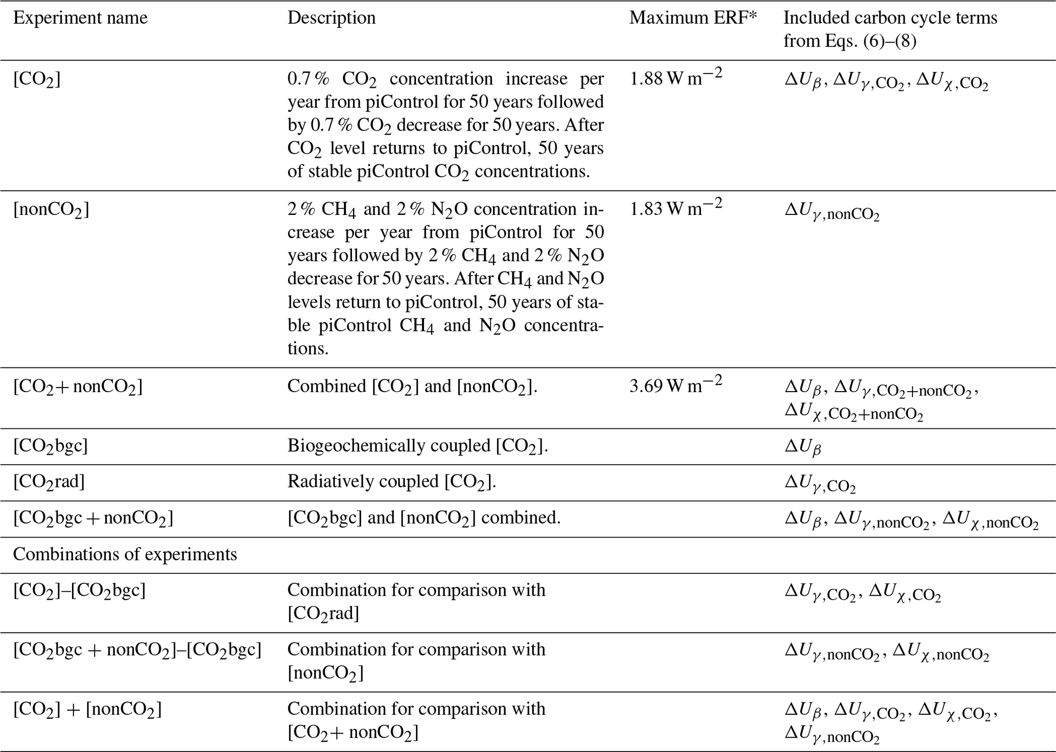
* According to equations by Etminan et al. (2016), warming from the physiological CO₂ forcing is assumed to be negligible.

The experiment design uses a fixed land cover and constant (other than CO₂, CH₄, and N₂O) GHG and aerosol forcings that might otherwise interfere with the interpretation of the results. The maximum ERF in our experiments is 3.69 W m⁻², as estimated from the equations by Etminan et al. (2016) (see also Appendix A), corresponding to an (actual) CO₂ concentration of 403 ppm, a CH₄ concentration of 2175 ppb, and an N₂O concentration of 735 ppb. This ERF level (very much in line with the current CO₂ concentration level of ca. 420 ppm) makes our experiments and results relevant to mitigation efforts in the near future. The small differences in ERF between the [CO₂] and [nonCO₂] experiments are not significant when considering ramp-up, ramp-down, and full periods at p<0.05.

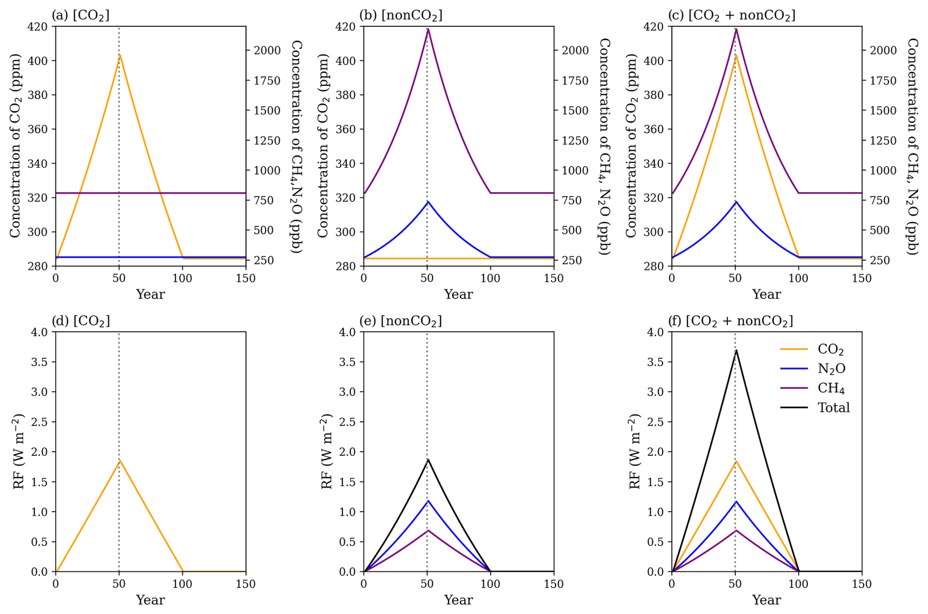
Figure 1 Time series of input (a)–(c) CO₂, CH₄, and N₂O concentrations and (d)–(f) their respective radiative ERFs according to the equations of Etminan et al. (2016) for (a, d) [CO₂], (b, e) [nonCO₂], and (c, f) [CO₂+ nonCO₂] experiments. Note the different scales on the y axes in panels (a)–(c) for CO₂ concentrations in ppm (left) and other GHG concentrations in ppb (right).

We investigate CO₂ and non-CO₂ impacts on the climate by looking at the differences between [CO₂] and [nonCO₂] experiments and [CO₂rad] and [nonCO₂] experiments, hereafter referred to as [CO₂]–[nonCO₂] and [CO₂rad]–[nonCO₂], respectively. The experiments manipulate CH₄ and N₂O concentrations simultaneously because our primary focus is to compare the effects of CO₂ with those of non-CO₂ gases (i.e. CH₄ and N₂O combined) in this study.

For each experiment, three ensemble members are branched from the years 1870, 2020, and 2170 of the CMIP6 piControl experiment, hereafter [piControl]. We note that the use of three members is not ideal, but it is a common compromise between computational cost and sampling the uncertainty due to climate variability. We estimate the changes relative to the corresponding [piControl] periods in order to avoid the effects of low-frequency internal climate variability from the piControl (Fig. S1 in the Supplement), as discussed in Bonnet et al. (2021). When reporting carbon sink/source in the following sections, we refer to the fluxes relative to the [piControl]. For diagnosing Atlantic Meridional Overturning Circulation (AMOC), we utilised the ocean overturning mass streamfunction in depth space (msftyz variable in CMIP6). Specifically, we calculated the maximum annual mean value of the streamfunction in the Atlantic basin north of 20° N through all of the model's depth layers (up to ca. 5800 m).

2.3 Carbon cycle feedback attribution

Traditionally, carbon cycle feedback analysis relies on fully coupled [CO₂], biogeochemically coupled [CO₂bgc], and radiatively coupled [CO₂rad] simulations (Arora et al., 2013, 2020; Friedlingstein et al., 2006; Gregory et al., 2009; Schwinger et al., 2014; Schwinger and Tjiputra, 2018; Williams et al., 2019; Zickfeld et al., 2011). The carbon uptake (ΔU) can then be derived using the well-established carbon cycle feedback framework as a sum of the carbon–concentration β parameter (GtC ppm⁻¹) multiplied by the changes in the atmospheric CO₂ concentration $\mathrm{\Delta }{C}_{{\mathrm{CO}}_{\mathrm{2}}}$ (ppm) and the carbon–climate γ feedback parameter (GtC K⁻¹) multiplied by the changes in surface temperature ΔT (K), using Eq. (1):

$$\begin{array}{}\text{(1)}& \mathrm{\Delta }U=\mathit{\beta }\times \mathrm{\Delta }{C}_{{\mathrm{CO}}_{\mathrm{2}}}+\mathit{\gamma }\times \mathrm{\Delta }T+\mathit{\epsilon }.\end{array}$$

Here, the term ε refers to a residual term.

The β parameter can be estimated from the [CO₂bgc]–[piControl], using Eq. (2):

$$\begin{array}{}\text{(2)}& \mathit{\beta }={\displaystyle \frac{\mathrm{\Delta }{U}_{\mathrm{BGC}}}{\mathrm{\Delta }{C}_{{\mathrm{CO}}_{\mathrm{2}}}}},\end{array}$$

where ΔU_BGC is the carbon uptake in the BGC experiment [CO₂bgc]. The β feedback reflects the changes in land and ocean carbon pools driven by the changes in CO₂ concentrations.

The γ parameter can be estimated from the [CO₂rad]–[piControl], using Eq. (3):

$$\begin{array}{}\text{(3)}& \mathit{\gamma }={\displaystyle \frac{\mathrm{\Delta }{U}_{\mathrm{RAD}}}{\mathrm{\Delta }T}},\end{array}$$

where ΔU_RAD is the carbon uptake in the RAD experiment [CO₂rad]. The γ feedback reflects the changes in the land and ocean carbon pools due to the changes in climate.

Many existing studies have estimated γ using the difference between the fully coupled (COU) and BGC experiments as a proxy for the RAD experiment (Arora et al., 2013, 2020; Asaadi et al., 2024; Friedlingstein et al., 2003, 2006; Melnikova et al., 2021). However, Zickfeld et al. (2011) and Schwinger et al. (2014) showed that this substitution introduces a residual term ε, which can be derived from the difference between [CO₂]–[CO₂bgc] and [CO₂rad]–[piControl] using Eq. (4):

$$\begin{array}{}\text{(4)}& \mathit{\epsilon }=\mathrm{\Delta }{U}_{\mathrm{COU}}-\mathrm{\Delta }{U}_{\mathrm{BGC}}-\mathrm{\Delta }{U}_{\mathrm{RAD}}.\end{array}$$

These studies indicate that the residual “nonlinearity” term depends on both CO₂ concentration and climate change, and it can be of the same order of magnitude as the γ term. Here, we propose that this residual nonlinearity be attributed to a cross-term, χ. Although recent studies continue to subsume χ under the γ feedback – partly due to the absence of the [CO₂rad] experiment in some experimental designs and also because this approach has been widely established in earlier research (Friedlingstein et al., 2003, 2006) – we show that these metrics become less well defined when examining the effects of both CO₂ and non-CO₂ GHGs on the carbon cycle.

In order to investigate the associated carbon–climate feedback nonlinearities, we propose the following theoretical framework. The changes in carbon uptake $\mathrm{\Delta }U(\mathrm{\Delta }{C}_{{\mathrm{CO}}_{\mathrm{2}}},\mathrm{\Delta }T)$ (GtC yr⁻¹) in the COU simulation can be defined as a function of changes in CO₂ concentration ($\mathrm{\Delta }{C}_{{\mathrm{CO}}_{\mathrm{2}}}$) and temperature (ΔT). Following Schwinger et al. (2014), the formulation can be expanded to a Taylor series up to the second-order terms:

$$\begin{array}{}\text{(5)}& \begin{array}{rl}\mathrm{\Delta }U& =\mathrm{\Delta }U\left(\mathrm{\Delta }{C}_{{\mathrm{CO}}_{\mathrm{2}}},\mathrm{\Delta }T\right)={\displaystyle \frac{\partial U}{\partial C_{{\mathrm{CO}}_{\mathrm{2}}}}}\mathrm{\Delta }{C}_{{\mathrm{CO}}_{\mathrm{2}}}+{\displaystyle \frac{\partial U}{\partial T}}\mathrm{\Delta }T\\ & +{\displaystyle \frac{{\partial }^{\mathrm{2}}U}{\partial C_{{\mathrm{CO}}_{\mathrm{2}}}\partial T}}\mathrm{\Delta }T\mathrm{\Delta }{C}_{{\mathrm{CO}}_{\mathrm{2}}}+{\displaystyle \frac{\mathrm{1}}{\mathrm{2}}}{\displaystyle \frac{{\partial }^{\mathrm{2}}U}{\partial C_{{\mathrm{CO}}_{\mathrm{2}}}^{\mathrm{2}}}}{\left(\mathrm{\Delta }{C}_{{\mathrm{CO}}_{\mathrm{2}}}\right)}^{\mathrm{2}}\\ & +{\displaystyle \frac{\mathrm{1}}{\mathrm{2}}}{\displaystyle \frac{{\partial }^{\mathrm{2}}U}{\partial T^{\mathrm{2}}}}(\mathrm{\Delta }T{)}^{\mathrm{2}}+\mathrm{Res},\end{array}\end{array}$$

where $\mathrm{\Delta }{C}_{{\mathrm{CO}}_{\mathrm{2}}}$ and ΔT_forc. are the respective increments of CO₂ concentration and temperature relative to [piControl]. The third- and higher-order terms are defined as a residual (Res.). We found them to be negligible in our case. We can disentangle the first- and second-order terms of the right-hand side of the Eq. (5) into terms that are purely dependent on CO₂ (ΔU_β), on temperature (ΔU_γ), and on the cross-term (ΔU_χ) as follows:

$$\begin{array}{}\text{(6)}& {\displaystyle }\mathrm{\Delta }{U}_{\mathit{\beta }}={\displaystyle \frac{\partial U}{\partial C_{{\mathrm{CO}}_{\mathrm{2}}}}}\mathrm{\Delta }{C}_{{\mathrm{CO}}_{\mathrm{2}}}+\mathrm{Res},\text{(7)}& {\displaystyle }\mathrm{\Delta }{U}_{\mathit{\gamma }}={\displaystyle \frac{\partial U}{\partial T}}\mathrm{\Delta }T+\mathrm{Res},\text{(8)}& {\displaystyle }\mathrm{\Delta }{U}_{\mathit{\chi }}={\displaystyle \frac{{\partial }^{\mathrm{2}}U}{\partial C_{{\mathrm{CO}}_{\mathrm{2}}}\partial T}}\mathrm{\Delta }T\mathrm{\Delta }{C}_{{\mathrm{CO}}_{\mathrm{2}}}+\mathrm{Res}.\end{array}$$

For simplicity, the second-order terms of Eqs. (6) and (7) are included in Res. Combining Eqs. (4) and (8), the χ feedback parameter may be quantified from

$$\begin{array}{}\text{(9)}& \mathit{\chi }={\displaystyle \frac{\mathrm{\Delta }{U}_{\mathrm{COU}-\mathrm{BGC}}-\mathrm{\Delta }{U}_{\mathrm{RAD}}}{\mathrm{\Delta }T\mathrm{\Delta }{C}_{{\mathrm{CO}}_{\mathrm{2}}}}}.\end{array}$$

The carbon–concentration β feedback term ΔU_β may be estimated from [CO₂bgc]–[piControl], under the assumption that the physiological CO₂ warming and its impacts on the carbon cycle are negligible, consistent with findings of Asaadi et al. (2024). The γ feedback terms for CO₂ ($\mathrm{\Delta }{U}_{\mathit{\gamma },{\mathrm{CO}}_{\mathrm{2}}}$) and non-CO₂ ($\mathrm{\Delta }{U}_{\mathit{\gamma },{\mathrm{nonCO}}_{\mathrm{2}}}$) gases are estimated from [CO₂rad]–[piControl] and [nonCO₂]–[piControl], respectively. The difference between these terms ($\mathrm{\Delta }{U}_{\mathit{\gamma },{\mathrm{CO}}_{\mathrm{2}}}$–$\mathrm{\Delta }{U}_{\mathit{\gamma },{\mathrm{nonCO}}_{\mathrm{2}}}$) yields the difference between impacts of CO₂ and non-CO₂ forcing on the carbon–climate feedback. Finally, the cross-term ΔU_χ, previously referred to as a nonlinearity term (Arora et al., 2013, 2020; Gregory et al., 2009; Schwinger et al., 2014; Schwinger and Tjiputra, 2018; Williams et al., 2019; Zickfeld et al., 2011), may be estimated by utilising a combination of experiments. The combination [CO₂]–[CO₂bgc]–[CO₂rad] gives $\mathrm{\Delta }{U}_{\mathit{\chi },{\mathrm{CO}}_{\mathrm{2}}}$, and the combination [CO₂bgc + nonCO₂]–[CO₂bgc]–[nonCO₂] gives $\mathrm{\Delta }{U}_{\mathit{\chi },{\mathrm{nonCO}}_{\mathrm{2}}}$. Analogously, the difference between these cross-terms ($\mathrm{\Delta }{U}_{\mathit{\chi },{\mathrm{CO}}_{\mathrm{2}}}-\mathrm{\Delta }{U}_{\mathit{\chi },{\mathrm{nonCO}}_{\mathrm{2}}}$) yields the difference between the CO₂ and non-CO₂ forcings on the χ.

3 Results and discussion

3.1 Climate impacts

The analysis of global climate variables as a function of CO₂ concentration and GSAT shown in Fig. 2 follows a previous study by Boucher et al. (2012). Consistent with their findings, our results show that GSAT change lags behind GHG forcing by up to 1 decade. The lag increases with the increase in the forcing magnitude so that the largest lag is in the [CO₂+ nonCO₂] experiment. Even after a ramp-down period and 50 years of constant GHG forcing at [piControl] levels, GSAT does not return to preindustrial values in all experiments (Fig. 2a). This can be explained by the inertia of the climate system, apparent in the changes in the ocean heat uptake (OHU). The OHU increases during the ramp-up and decreases during the ramp-down period, being positive, i.e. taking up energy away from the atmosphere, during the ramp-up and the first half of the ramp-down period. OHU turns negative by the end of the ramp-down and stays negative during the 50 years of the stabilisation period, releasing energy back into the atmosphere (Fig. 2c–e). The hysteresis of the climate system is evident from the nearly linear relationship between maximum GSAT and mean GSAT during the stabilisation period (Fig. S2). The thermosteric (unrelated to ice sheet melting) sea level increases in all experiments except for [CO₂bgc] and is closely related to the OHU. It does not recover (i.e. it is irreversible) within the time horizon considered here (Fig. 2i–k). The AMOC decreases with GSAT (with the strongest decrease reached for GSAT of 2 °C under [CO₂+ nonCO₂]) but fully recovers (Fig. S1b).

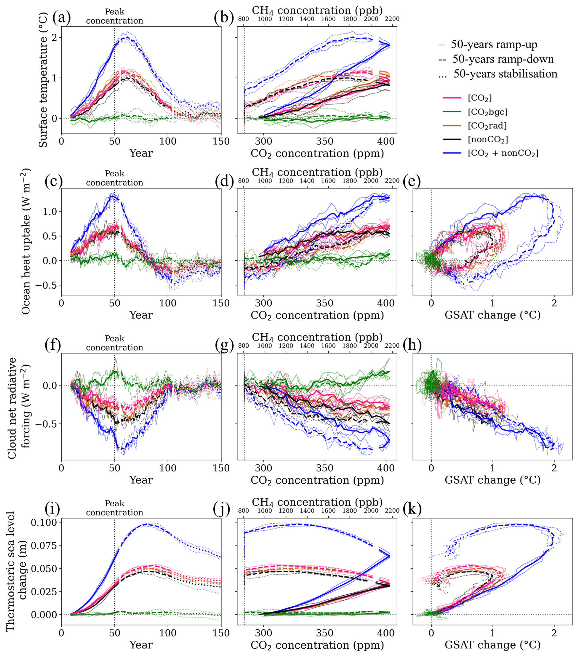
Figure 2 Global annual mean changes in model climate variables as a function of (a, c, f, i) time (year), (b, d, g, j) CO₂ concentration $\left(\mathrm{ppm}\right)/{\mathrm{CH}}_{\mathrm{4}}$ concentration (ppb; only for [nonCO₂]), and (c, e, h, k) GSAT (°C) for (a, b) GSAT (°C), (c–e) ocean heat uptake (W m⁻²), (f–h) cloud net radiative forcing (W m⁻²), and (i–k) thermosteric sea level change (m) under selected scenarios. The ramp-up, ramp-down, and stabilisation periods are indicated by different line styles in all panels. Thick lines indicate the ensemble means, and thin lines correspond to three ensemble members.

The CO₂ physiological warming that can be quantified by comparing [CO₂bgc] with [piControl] is small (green line in Fig. 2). Spatially, some differences are ubiquitous over land, e.g. CO₂ physiological warming persists over Eurasia during the ramp-up period, and over the high latitudes of both land and ocean during the stabilisation period (Fig. S3a). A larger ensemble size of model simulations would be required to investigate these differences more thoroughly. In our following analysis on carbon cycle feedbacks, we assume the CO₂ physiological warming to be negligible, consistent with previous findings of Asaadi et al. (2024).

When comparing CO₂- and non-CO₂-induced forcing ([CO₂] and [nonCO₂] experiments) at a global scale, our results are consistent with Richardson et al. (2019), who show the higher surface temperature response of CO₂ when compared to CH₄. When comparing CO₂- and non-CO₂-induced radiative forcing ([CO₂rad] and [nonCO₂] experiments) at a global scale, the non-CO₂ forcing still leads to a lower GSAT peak and a slightly lower peak of thermosteric sea level rise compared to the CO₂ radiative forcing (brown and black lines of Fig. 2a, significant difference at p<0.05). This cannot be explained just by a slightly higher ERF of the [CO₂rad] compared to the [nonCO₂] experiment (Table 1, Figs. 2a and S4). Our results are consistent with Nordling et al. (2021), who show the higher effective temperature response for CO₂ forcing compared to non-CO₂ forcing, attributing it to the changes in clear-sky planetary emissivity.

Radiative forcing alone ([CO₂rad] experiment) leads to a slightly higher global temperature increase compared to the coupled [CO₂] experiment, which includes the combined effect of CO₂ physiology and radiative forcing (Fig. 2a, b). This temperature difference is particularly evident in the Arctic region (Fig. S3a). Our findings differ from those of a CMIP5 intercomparison study, which reported that CO₂ physiological warming amplifies the Arctic warming (Park et al., 2020). The study showed that the CO₂ physiological effect contributes to high-latitude warming by reducing evaporative cooling due to stomatal closure under elevated CO₂ levels. In contrast, we observe higher evapotranspiration in the [CO₂rad] compared to the [CO₂] experiment (Fig. S5), which is probably a consequence of the lower warming in the [CO₂] experiment. In our study, the greater warming in the [CO₂rad] experiment may be driven by increased surface albedo, especially in the Arctic Ocean (Fig. S3b). While the underlying causes remain unclear, this pattern appears consistent in other experiments conducted with IPSL-CM6A-LR under moderate CO₂ levels (not shown). Because the ensemble size in our study is limited and the effects of the model's internal variability should be considerable, future research should validate the robustness of our findings with larger ensemble simulations.

3.2 Carbon cycle feedback

3.2.1 Carbon–concentration feedback

The term $\mathrm{\Delta }{U}_{\mathit{\beta },{\mathrm{CO}}_{\mathrm{2}}}$ corresponds to the flux arising from variations in CO₂ concentration ([CO₂bgc] experiment). The $\mathrm{\Delta }{U}_{\mathit{\beta },{\mathrm{CO}}_{\mathrm{2}}}$ dominates the land and ocean carbon uptake changes through all three considered periods (Fig. 3, Tables 2 and S1). Since the considered maximum surface warming levels are below 2 °C, land and ocean carbon fluxes are primarily controlled by the CO₂-induced effects during the ramp-up period, resulting in positive β (Fig. 3a–d). Nearly two-thirds of land and half of ocean carbon accumulated during the ramp-up period due to the atmospheric CO₂ increase are being released during the latter periods, consistent with previous studies (Asaadi et al., 2024; Chimuka et al., 2023). In the ocean, β is positive (carbon sink) in all regions during the ramp-up period. However, a decrease in CO₂ concentration induces a carbon source over all ocean regions, except for the Atlantic and Southern oceans (Fig. 4). All regions are carbon sources during the stabilisation period of the [CO₂bgc] experiment.

Table 2 Cumulative CO₂ and climate-change-driven changes in the land and ocean carbon fluxes (GtC), shown as a three-member ensemble mean. The ± indicates 1 standard deviation among the three members. Note that all experiments are analysed relative to their [piControl] counterparts.

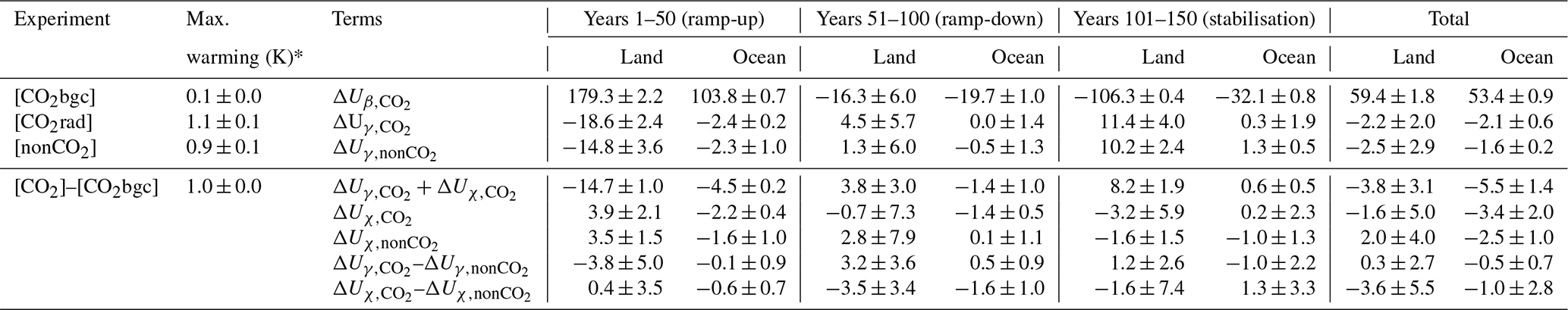
* Defined as the mean ΔGSAT during years 41–60 in the experiments.

The transient change in the β feedback over land can be better explained by analysing the gross primary production (GPP) and the autotrophic and heterotrophic respiration (Ra and Rh) fluxes. Land GPP, representing photosynthetic uptake, increases during the ramp-up period under elevated CO₂ concentration and decreases almost linearly with decreasing CO₂, showing only a small hysteresis (Figs. S6–S7). In contrast, both Ra and Rh exhibit a larger hysteresis, which leads to an extended period of the carbon release to the atmosphere. This suggests that, while there may be initial carbon sequestration benefits gained during elevated CO₂ periods, these benefits are susceptible to being lost as CO₂ concentrations decline due to decreased photosynthesis and increased respiration, albeit at a reduced rate.

The spatial variation in cumulative net carbon uptake provides further details on the feedback changes (Figs. 4, S8–S10). During the CO₂ ramp-up phase, CO₂ increase triggers a land carbon sink in all regions. However, during the ramp-down phase, it induces a net carbon source over subtropical regions while still driving a land carbon sink in northern high latitudes so that global land becomes a carbon source in the middle of the ramp-down phase. Finally, during the stabilisation period, all land regions become net carbon sources.

Subtropical and southern land regions exhibit a shorter hysteresis in response to decreasing CO₂ concentrations. This disparity arises from the larger proportion of carbon accumulated in aboveground vegetation biomass in southern regions, contrasting with the greater fraction stored in soils within northern latitudes (Figs. S9–S11). The extended period of high positive β in northern mid- to high latitudes can be attributed to the longer carbon turnover time, particularly in soils, compared to tropical regions (Fig. S8).

3.2.2 Carbon–climate feedback

The term ΔU_γ corresponds to the carbon flux arising from variations in radiative forcing (such as in the [nonCO₂] and [CO₂rad] experiments). The ΔU_γ for CO₂ and non-CO₂ ($\mathrm{\Delta }{U}_{\mathit{\gamma },{\mathrm{CO}}_{\mathrm{2}}}$ and $\mathrm{\Delta }{U}_{\mathit{\gamma },{\mathrm{nonCO}}_{\mathrm{2}}}$, respectively) are equivalent (within 1 standard deviation uncertainty range) under nearly equivalent levels of ERF (compare panels b and c of Fig. 4; see also $\mathrm{\Delta }{U}_{\mathit{\gamma },{\mathrm{CO}}_{\mathrm{2}}}$–$\mathrm{\Delta }{U}_{\mathit{\gamma },{\mathrm{nonCO}}_{\mathrm{2}}}$ in Table 2 and Table S1). The γ is negative on a global scale in the land and ocean, with greater magnitude but also faster reversibility over land. Spatially, land γ is positive in the mid- to high latitudes and negative in the tropical regions (Figs. 4, S9–10; see also Melnikova et al., 2021). During the ramp-up, climate change drives carbon sink in the northern mid- to high latitudes and carbon source in the subtropical regions and the Southern Hemisphere, with a larger magnitude of changes in the experiments, in which CO₂ concentration change is present (Figs. 4, S9–11).

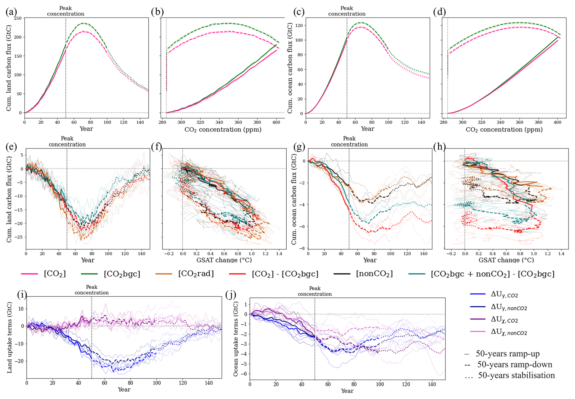
Figure 3 Global cumulative carbon fluxes (GtC) over (a, b, e, f, i) land and (c, d, g, h, j) ocean as a function of (a, c, e, g, i, j) time (year), (b, d) CO₂ concentration (ppm), and (f, h) GSAT changes (°C) under selected scenarios. The ramp-up, ramp-down, and stabilisation periods are indicated by different line styles. Thick lines indicate the ensemble means, and thin lines correspond to other ensemble members. Note that vertical axes differ between panels (e) and (g) and panels (i) and (j).

3.2.3 Nonlinearity in carbon cycle feedback

The cross-term ΔU_χ induces non-negligible differences between climate-change-induced carbon flux when comparing experiments with the presence or absence of atmospheric CO₂ concentration change. It reaches ca. 20 %–23 % of the land ΔU_γ and ca. 70 %–90 % of the ocean ΔU_γ, cumulative over the ramp-up period (Table 2). During the ramp-up phase, the ΔU_χ corresponds to a decrease in the climate-driven land carbon source and an increase in the climate-driven ocean carbon source (Fig. 3). The χ feedback is positive (larger carbon sink) on land and negative (larger carbon source) in the ocean (Table S1). There is no significant difference between CO₂ and non-CO₂ χ feedback at similar ERF levels (Figs. 3e–j and 4f–g, Tables 2 and S1). In the ocean, the cross-term differences for CO₂ and non-CO₂ forcing already arise during the ramp-up and propagate during the ramp-down and stabilisation phases, spatially concentrating in the deep-mixing region of the Southern Ocean.

On land, the positive χ reflects more biomass at high latitudes available for climate change effects, leading to a larger carbon sink (positive γ). During the ramp-down, climate warming through temperature change (lagged after GHG concentrations change) increases the carbon sink over high latitudes and weakens the carbon source in the tropics. Here, the ΔU_χ reflects more biomass available globally for the climate change effects, leading to a larger carbon source (negative γ). The differences (in the presence/absence of the cross-term ΔU_χ) diminish for land but not for the ocean during the ramp-down and stabilisation periods.

In the ocean, the contribution from the nonlinearity of carbon cycle feedbacks leads to a greater reduction in the CO₂-driven carbon sink (Fig. 3). The contribution of the cross-term ΔU_χ to the total ΔU increases during the ramp-down phases of considered GHG concentration scenarios. Previously, Schwinger and Tjiputra (2018), who considered nonlinearity of carbon cycle feedback, warned that RAD experiments may underestimate the carbon–climate feedback (when compared to COU–BGC experiments) because “the reduction of sequestration of preformed dissolved inorganic carbon under high atmospheric CO₂ is not taken into account.” In this study, the nonlinearity effects nearly double climate-change-driven carbon loss (compared to the RAD experiment, in which atmospheric CO₂ is constant) relative to the total 150-year net ocean carbon uptake under the [CO₂] experiment. Spatially, while the Southern Ocean remains the largest ocean carbon sink in all considered experiments involving atmospheric CO₂ changes, it, along with the Atlantic Ocean, undergoes the largest climate-change-driven reduction in carbon sink (Fig. 4).

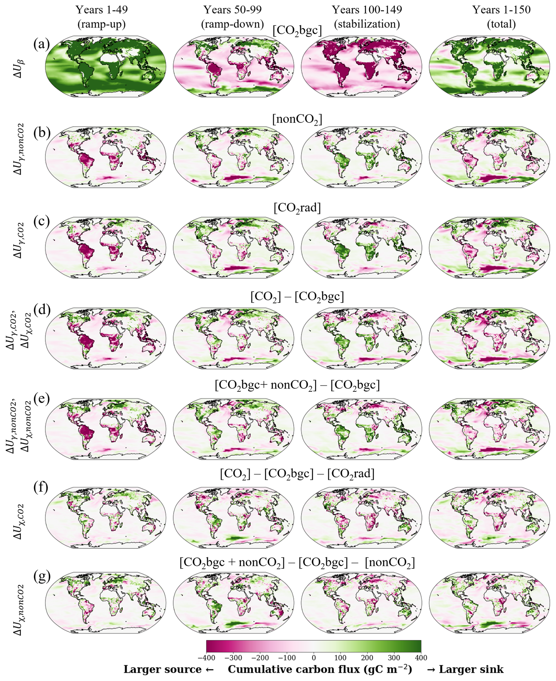
Figure 4 Spatial variation in land and ocean carbon fluxes (GtC, negative to the atmosphere) cumulative over 50 years of (first column) ramp-up (second column) and ramp-down (third column) stabilisation phases and (last column) the full 150-year period. The data for the three-member ensemble mean are used.

Our findings provide evidence on the effectiveness of non-CO₂ GHG mitigation. While it can effectively reduce GSAT peak, non-CO₂ GHG mitigation may also lead to smaller climate-change-driven losses in the ocean carbon sink. In the real world, the presence/absence of ΔU_χ suggests disparities between CO₂ mitigation efforts and non-CO₂ mitigation efforts. The CO₂- and non-CO₂-driven climate change leads to an unequal decrease in carbon uptake, especially apparent for the ocean on a global scale (compare red and black lines in Fig. 3, corresponding to [CO₂]–[CO₂bgc] and [nonCO₂] experiments). Reducing CO₂ concentrations for climate mitigation implies alteration of all three terms of the proposed carbon cycle feedback attribution framework, namely ΔU_β, ΔU_γ, and ΔU_χ. Reducing non-CO₂ GHG concentrations, such as CH₄ and N₂O, implies alteration of ΔU_γ and ΔU_χ terms. Reducing both CO₂ and non-CO₂ concentrations implies alteration of all ΔU_β, ΔU_γ, and ΔU_χ terms but with larger change in ΔU_γ and ΔU_χ terms. From this point, combining CO₂ and non-CO₂ reduction measures may be more effective for climate change mitigation compared to the CO₂ reduction measures alone. This finding should be confirmed with emission-driven experiments that consider GHG atmospheric lifetimes.

3.3 Radiative forcing and carbon cycle feedback additivity

In order to overcome the small signal-to-noise ratio of the considered experiments and the regional differences in the radiative forcing between [CO₂] and [nonCO₂] experiments, we compare (1) the [CO₂+ nonCO₂] experiment that includes both CO₂ and non-CO₂ effects with (2) the sum of two [CO₂] and [nonCO₂] experiments that include CO₂ and non-CO₂ effects, accordingly (Figs. 5 and S12–13). The climate effects, defined via temperature change, differ during the ramp-up and ramp-down periods (Fig. S12). These differences imply non-additivity of radiative forcing and can also be attributed to biophysical feedback.

As for the carbon cycle feedback, the [CO₂+ nonCO₂] experiment that has all feedback is different from the sum of two experiments [CO₂] + [nonCO₂] both on land and in the ocean (Fig. 5). The differences are larger and stay longer in the ocean. This implies non-additivity of carbon cycle feedback. From the proposed carbon cycle feedback attribution framework, the non-additivity arises from non-equality of ($\mathrm{\Delta }{U}_{\mathit{\gamma },{\mathrm{CO}}_{\mathrm{2}}+{\mathrm{nonCO}}_{\mathrm{2}}}+\mathrm{\Delta }{U}_{\mathit{\chi },{\mathrm{CO}}_{\mathrm{2}}+{\mathrm{nonCO}}_{\mathrm{2}}}$) and ($\mathrm{\Delta }{U}_{\mathit{\gamma },{\mathrm{CO}}_{\mathrm{2}}}+\mathrm{\Delta }{U}_{\mathit{\chi },{\mathrm{CO}}_{\mathrm{2}}}+\mathrm{\Delta }{U}_{\mathit{\gamma },{\mathrm{nonCO}}_{\mathrm{2}}}+\mathrm{\Delta }{U}_{\mathit{\chi },{\mathrm{nonCO}}_{\mathrm{2}}}$). The significant difference (p<0.1) on land is in the high-latitude region, where the “all-effects together” [CO₂+ nonCO₂] experiment yields a larger carbon sink during the ramp-up phase. The largest difference in the ocean is in the Southern Ocean, followed by the North Atlantic Ocean. The [CO₂+ nonCO₂] experiment has a large carbon sink in the Southern Ocean compared to the sum of two experiments. This might be related to the saturation of the decrease in the mixed-layer depth with more warming, but a more thorough study is needed to confirm such phenomena.

4 Limitations and future research directions

To our knowledge, this is the first study of its kind to compare idealised CO₂ and non-CO₂ ramp-up and ramp-down scenarios for their effects on global temperature change and the carbon cycle feedbacks. Below we draw attention to the caveats and limitations that should be addressed in future studies.

Firstly, since IPSL-CM6A-LR, like all other ESMs participating in CMIP6, does not have interactive modules of the CH₄ and N₂O cycles, the changes in stratospheric water vapour, aerosols, and tropospheric ozone due to atmospheric CH₄ changes and the effects of nitrogen deposition on the carbon cycle are not considered in this study. Future studies could separately consider simulations for CH₄ and N₂O. However, for this study, the use of the model is justified because current changes in CH₄ and N₂O concentrations are primarily driven by anthropogenic sources, suggesting that the absence of interactive modules of natural sink/source processes does not significantly affect the representation of natural variability trends for the CH₄ and N₂O concentration (Nakazawa, 2020; Palazzo Corner et al., 2023; Zhu et al., 2013).

Secondly, when interpreting the results, it should be kept in mind that some carbon cycle processes in IPSL-CM6A-LR, such as permafrost and fire, are not considered. However, these should have only a limited impact on our results, given the (relatively) small warming levels in the considered experiments. Previous studies have shown that IPSL-CM6A-LR estimates one of the smallest soil carbon pools among CMIP6 models, which may lead to an underestimation of the carbon–climate feedback (Arora et al., 2020; Melnikova et al., 2021).

Thirdly, the results of the present study are limited by the use of a single ESM and a small number of ensemble members. Conducting similar experiments with other ESMs and using larger ensemble runs, which are particularly valuable in the low-warming scenarios, and complementing the findings of our study with emission-driven experiments could contribute to validating and extending our findings.

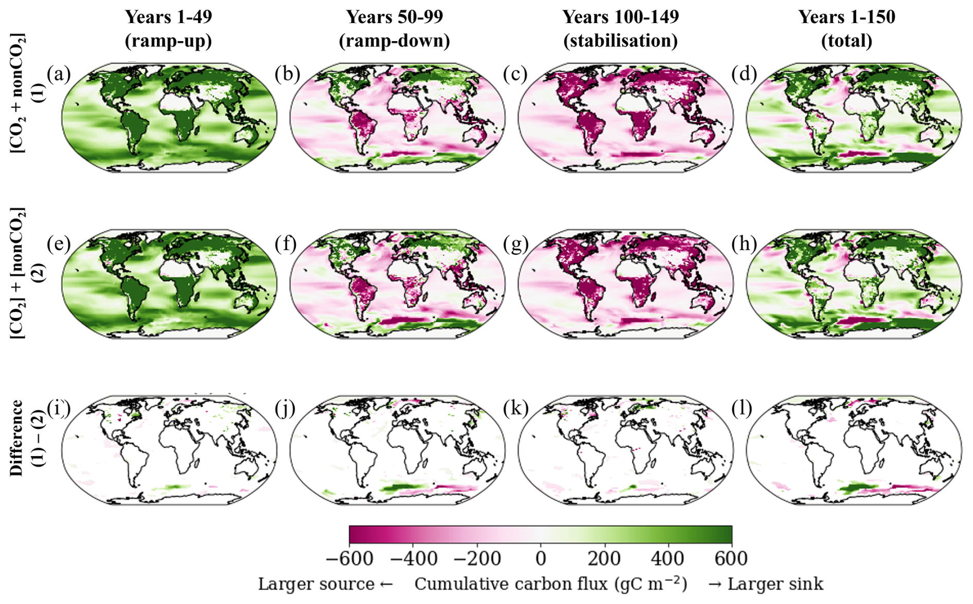
Figure 5 Spatial variation in three-member ensemble mean land and ocean carbon fluxes (GtC, negative to the atmosphere) cumulative over 50 years of (a, e, i) ramp-up, (b, f, j) ramp-down, (c, g, k) stabilisation phases, and (d, h, l) the full 150-year period. We draw only significantly different grids between (i–l) [CO₂+ nonCO₂] and [CO₂] + [nonCO₂] experiments using three ensemble members (p<0.1 based on t-test, N=60).

5 Conclusions

This study first presents a novel approach to recalibrate the ERF of CH₄ and N₂O in ESMs without changing the radiative scheme of the model. We then discuss the effects of increases and decreases in the concentrations of the CO₂ and non-CO₂ GHGs on the surface climate and carbon cycle. We find only small differences between CO₂ and non-CO₂ ramp-up and ramp-down forcing on global and regional climate.

The differences in climate responses can be linked to differences in the carbon cycle feedbacks. We show that CO₂- and non-CO₂-driven carbon–climate feedback are nearly equivalent at a global scale. However, increasing atmospheric CO₂ amplifies the reduction in the climate-change-driven carbon sink, especially in the ocean. We propose a novel framework to disentangle the carbon–climate feedback into a component that is purely driven by climate change, i.e. expressed as a temperature term, and a component driven by climate change and rising atmospheric CO₂ at the same time, i.e. a cross-term. Since the cross-term can be quantified from the difference between COU, BGC, and RAD simulations, we advocate for continuing to carry out all three types of experiments in the future phases of CMIP. We further warn that the cross-term and non-additivity of feedback should be considered in the simple climate models (emulators).

Finally, this study showcases the additional benefits of non-CO₂ GHG mitigation on a smaller reduction in the ocean carbon sinks under overshoot scenarios. We stress that our findings do not imply that non-CO₂ GHG mitigation should be given a priority over other means to mitigate climate change but that they provide insights on the intricate interplay between the carbon–concentration and CO₂- and non-CO₂-driven carbon–climate feedbacks to inform comprehensive mitigation strategies.

Appendix A

A set of 40-year idealised IPSL-CM6A-LR simulations (840 years in total) has been carried out. In these experiments, the sea surface temperature (SST) and sea ice fractions were fixed to their preindustrial levels. CH₄ concentration levels were kept at 2× CH₄, 3× CH₄, 4× CH₄, 5× CH₄, 8× CH_4, and 12× CH₄, and N₂O concentration levels were kept at 1× N₂O, 1.25× N₂O, 1.5× N₂O, and 1.75× N₂O (Table A1).

Table A1 Description of idealised recalibration experiments using IPSL-CM6A-LR.

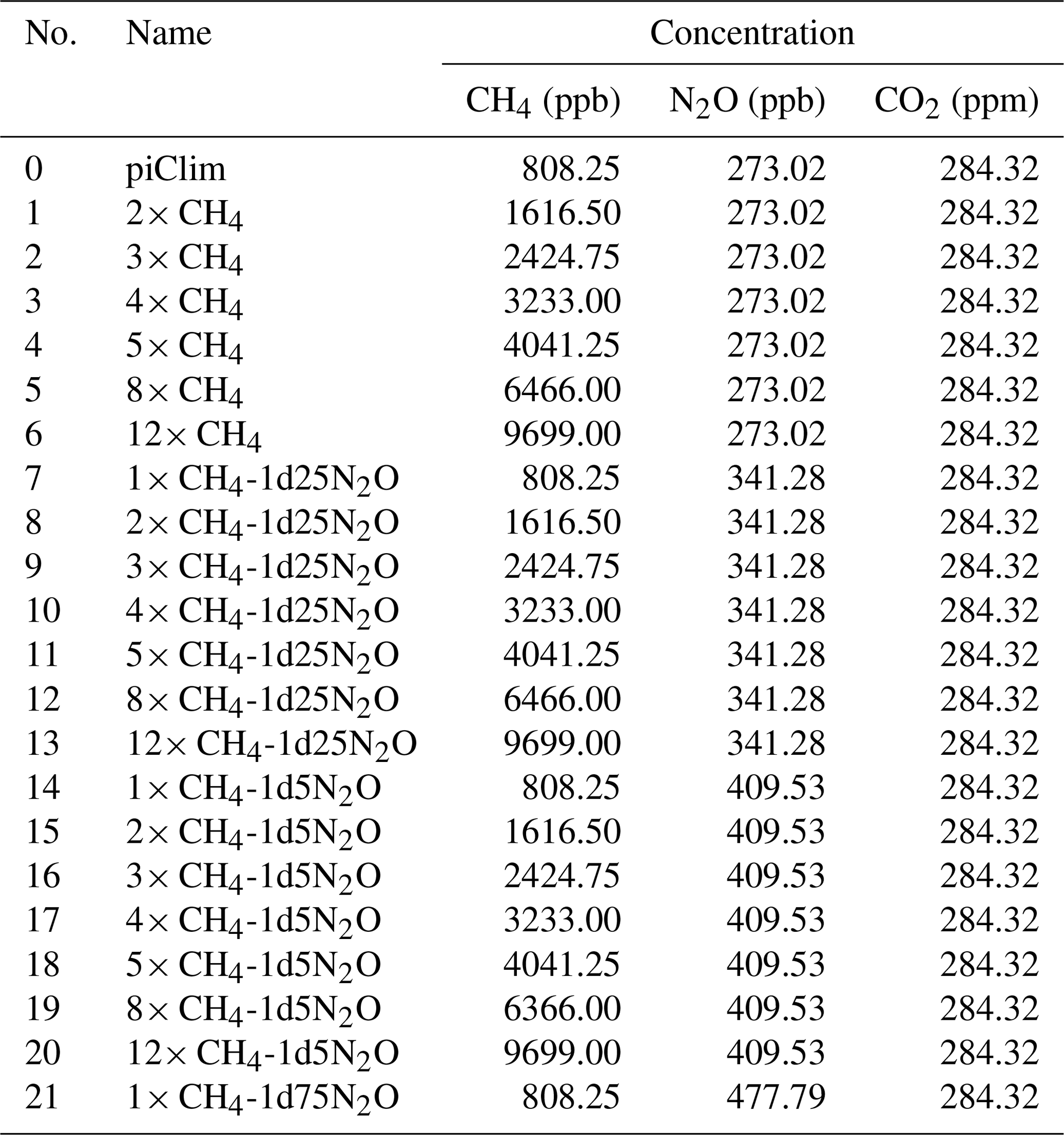
Figure A1 shows the set of 40-year time series of global mean radiative forcing based on 21 idealised experiments. The piClim experiment holds preindustrial levels of CO₂, CH₄, and N₂O concentrations. The mean interannual variation in the radiative forcings (1 standard deviation) is 0.15 W m⁻². The first 10 years of the experiments were dropped to allow the climate to adjust to the new radiative equilibrium after an abrupt change from the preindustrial levels. The last 30 years were used to obtain 18 data points of mean global ERF by IPSL-CM6A-LR relative to the levels obtained from the piClim experiment. The ERF is estimated as a TOA imbalance difference between each experiment and the piClim.

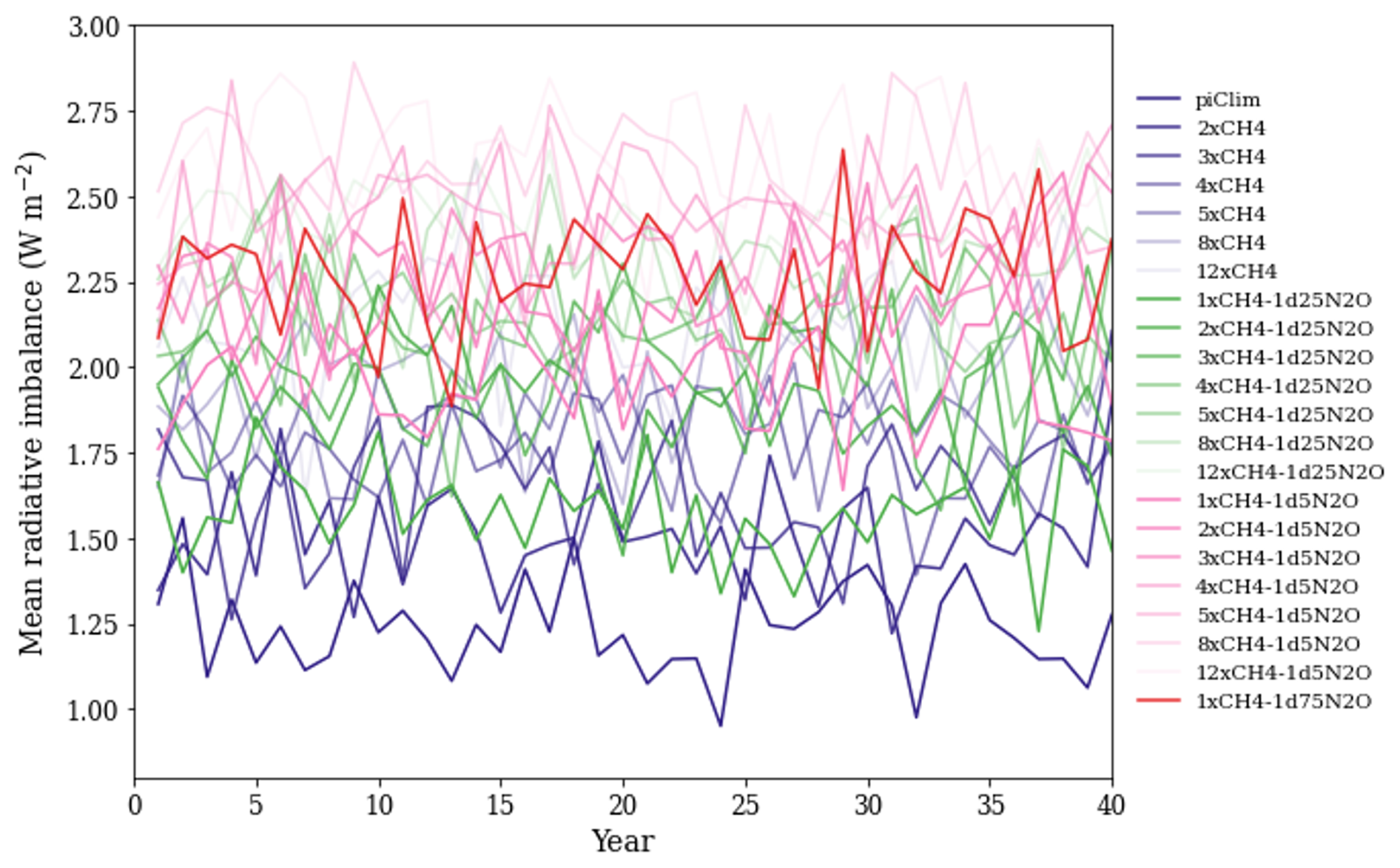
Figure A1 Time series of global mean radiative imbalance of IPSL-CM6A-LR idealised experiments.

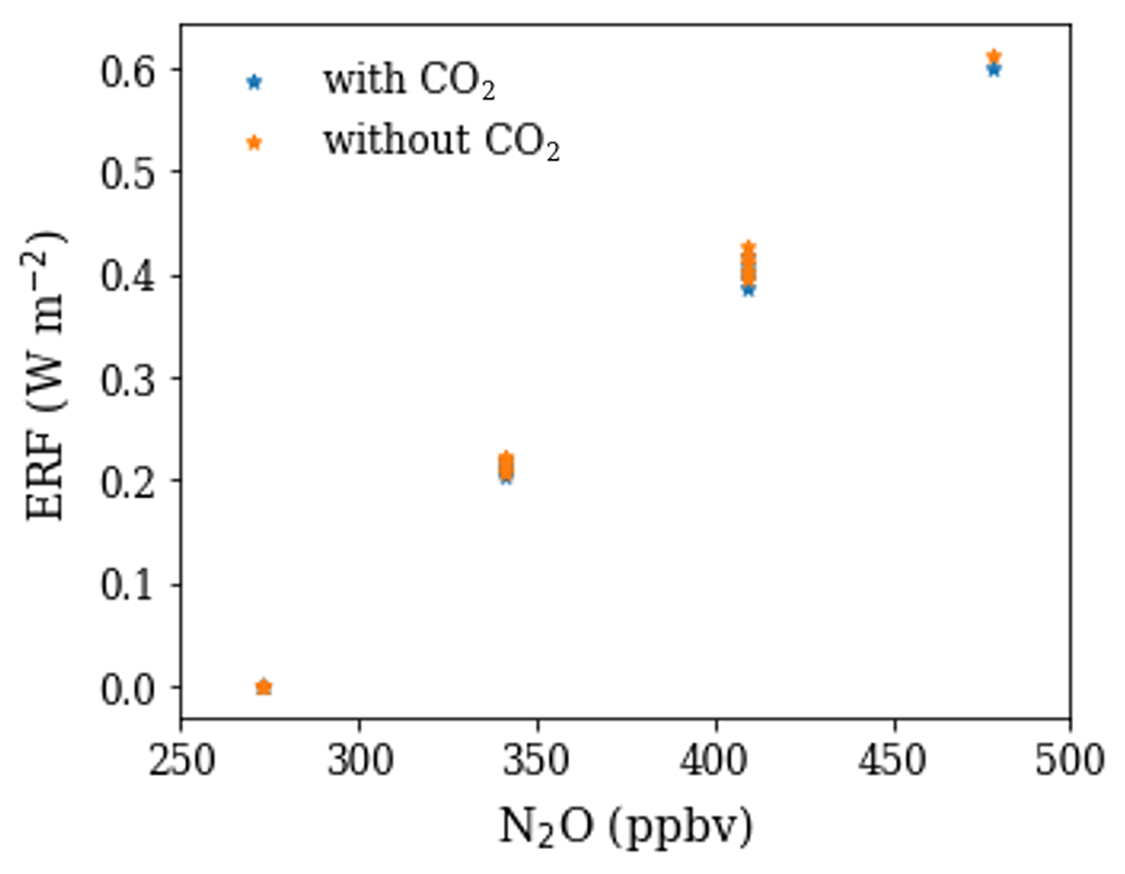
Figure A2 The ERF estimated from E16 with and without accounting for CO₂ impact on the N₂O forcing (including/excluding the term $-\mathrm{80}\times {\mathrm{10}}^{-\mathrm{6}}\times \mathrm{05}\times \left({\mathrm{CO}}_{\mathrm{2}}+{\mathrm{CO}}_{\mathrm{2},t=\mathrm{0}}\right)$ in the equation) using the concentration values of the idealised experiments described in Table 1 with preindustrial CO₂ concentration (284.32 ppm) and the same set of the experiments with 3 × CO₂ concentration (852.96 ppm).

There are two frequently used sets of equations to derive radiative forcing of well-mixed greenhouse gases, e.g. CO₂, CH₄, and N₂O, based on their concentrations. The first set from Myhre et al. (1998; hereafter, M98) was used in IPCC AR3:

$$\begin{array}{rl}& \mathrm{RF}\left({\mathrm{CO}}_{\mathrm{2}}\right)=\mathrm{5.35}\times \ln ({\mathrm{CO}}_{\mathrm{2}}/{{\mathrm{CO}}_{\mathrm{2}}}_{t=\mathrm{0}})\\ & \mathrm{RF}\left({\mathrm{CH}}_{\mathrm{4}}\right)=\mathrm{0.036}\times \left(\sqrt{{\mathrm{CH}}_{\mathrm{4}}}-{\sqrt{{\mathrm{CH}}_{\mathrm{4}}}}_{t=\mathrm{0}}\right)\\ & -\left(f\left({\mathrm{CH}}_{\mathrm{4}},{{\mathrm{N}}_{\mathrm{2}}\mathrm{O}}_{t=\mathrm{0}}\right)-f\left({{\mathrm{CH}}_{\mathrm{4}}}_{t=\mathrm{0}},{{\mathrm{N}}_{\mathrm{2}}\mathrm{O}}_{t=\mathrm{0}}\right)\right)\end{array}$$

$$\begin{array}{}\text{(A1)}& \begin{array}{rl}& \mathrm{RF}\left({\mathrm{N}}_{\mathrm{2}}\mathrm{O}\right)=\mathrm{0.12}\times \left(\sqrt{{\mathrm{N}}_{\mathrm{2}}\mathrm{O}}-{\sqrt{{\mathrm{N}}_{\mathrm{2}}\mathrm{O}}}_{t=\mathrm{0}}\right)\\ & -\left(f\left({{\mathrm{CH}}_{\mathrm{4}}}_{t=\mathrm{0}},{\mathrm{N}}_{\mathrm{2}}\mathrm{O}\right)-f\left({{\mathrm{CH}}_{\mathrm{4}}}_{t=\mathrm{0}},{{\mathrm{N}}_{\mathrm{2}}\mathrm{O}}_{t=\mathrm{0}}\right)\right)\\ & f\left({\mathrm{CH}}_{\mathrm{4}},{\mathrm{N}}_{\mathrm{2}}\mathrm{O}\right)=\mathrm{0.47}\times \ln \left[\mathrm{1}+\mathrm{2.01}\times {\mathrm{10}}^{-\mathrm{5}}\right.\\ & \times {\left({\mathrm{CH}}_{\mathrm{4}}\times {\mathrm{N}}_{\mathrm{2}}\mathrm{O}\right)}^{\mathrm{0.75}}+\mathrm{5.31}\times {\mathrm{10}}^{-\mathrm{15}}\\ & \left.\times {\mathrm{CH}}_{\mathrm{4}}\times {\left({\mathrm{CH}}_{\mathrm{4}}\times {\mathrm{N}}_{\mathrm{2}}\mathrm{O}\right)}^{\mathrm{1.52}}\right].\end{array}\end{array}$$

Here, the CO₂, CH₄, and N₂O indicate their concentrations, where the units are ppm, ppb, and ppb, respectively.

Etminan et al. (2016; hereafter, E16) improved the IPCC AR3 equations by inclusion of the short-wave (near-infrared) bands of CH₄. Their set of equations was used in IPCC AR6. The radiative forcing of N₂O in the M98 equation depends on the CH₄ and N₂O concentrations, while the radiative forcing of N₂O in the equation by E16 depends on the CO₂, CH₄, and N₂O concentrations:

$$\begin{array}{rl}& \mathrm{RF}\left({\mathrm{CO}}_{\mathrm{2}}\right)=\left[-\mathrm{2.4}\times {\mathrm{10}}^{-\mathrm{7}}\times {\left({\mathrm{CO}}_{\mathrm{2}}-{{\mathrm{CO}}_{\mathrm{2}}}_{t=\mathrm{0}}\right)}^{\mathrm{2}}+\mathrm{7.2}\right.\\ & \times {\mathrm{10}}^{-\mathrm{4}}\times \left|{\mathrm{CO}}_{\mathrm{2}}-{{\mathrm{CO}}_{\mathrm{2}}}_{t=\mathrm{0}}\right|-\mathrm{2.1}\times {\mathrm{10}}^{-\mathrm{4}}\times {\displaystyle \frac{\mathrm{1}}{\mathrm{2}}}\\ & \left.\left({\mathrm{N}}_{\mathrm{2}}\mathrm{O}+{{\mathrm{N}}_{\mathrm{2}}\mathrm{O}}_{t=\mathrm{0}}\right)+\mathrm{5.36}\right]\ln \left({\displaystyle \frac{{\mathrm{CO}}_{\mathrm{2}}}{{{\mathrm{CO}}_{\mathrm{2}}}_{t=\mathrm{0}}}}\right)\\ & \mathrm{RF}\left({\mathrm{CH}}_{\mathrm{4}}\right)=\left[-\mathrm{1.3}\times {\mathrm{10}}^{-\mathrm{6}}\times {\displaystyle \frac{\mathrm{1}}{\mathrm{2}}}\left({\mathrm{CH}}_{\mathrm{4}}+{{\mathrm{CH}}_{\mathrm{4}}}_{t=\mathrm{0}}\right)-\mathrm{8.2}\times {\mathrm{10}}^{-\mathrm{6}}\right.\\ & \left.\times {\displaystyle \frac{\mathrm{1}}{\mathrm{2}}}\left({\mathrm{N}}_{\mathrm{2}}\mathrm{O}+{{\mathrm{N}}_{\mathrm{2}}\mathrm{O}}_{t=\mathrm{0}}\right)+\mathrm{0.043}\right]\times \left(\sqrt{{\mathrm{CH}}_{\mathrm{4}}}-\sqrt{{{\mathrm{CH}}_{\mathrm{4}}}_{t=\mathrm{0}}}\right)\end{array}$$

$$\begin{array}{}\text{(A2)}& \begin{array}{rl}& \mathrm{RF}\left({\mathrm{N}}_{\mathrm{2}}\mathrm{O}\right)=\left[-\mathrm{8.0}\times {\mathrm{10}}^{-\mathrm{6}}\times {\displaystyle \frac{\mathrm{1}}{\mathrm{2}}}\left({\mathrm{CO}}_{\mathrm{2}}+{{\mathrm{CO}}_{\mathrm{2}}}_{t=\mathrm{0}}\right)\right.\\ & +\left(\mathrm{4.2}\times {\mathrm{10}}^{-\mathrm{6}}\times {\displaystyle \frac{\mathrm{1}}{\mathrm{2}}}\left({\mathrm{N}}_{\mathrm{2}}\mathrm{O}+{{\mathrm{N}}_{\mathrm{2}}\mathrm{O}}_{t=\mathrm{0}}\right)\right)-\mathrm{4.9}\times {\mathrm{10}}^{-\mathrm{6}}\\ & \times {\displaystyle \frac{\mathrm{1}}{\mathrm{2}}}\left.\left({\mathrm{CH}}_{\mathrm{4}}+{{\mathrm{CH}}_{\mathrm{4}}}_{t=\mathrm{0}}\right)+\mathrm{0.117}\right]\times \\ & \left(\sqrt{{\mathrm{N}}_{\mathrm{2}}\mathrm{O}}-\sqrt{{{\mathrm{N}}_{\mathrm{2}}\mathrm{O}}_{t=\mathrm{0}}}\right).\end{array}\end{array}$$

In the sets of Eq. (A2), the radiative forcing due to CH₄ depends not only on the CH₄ concentration but also on that of N₂O (and conversely) because CH₄ and N₂O absorption bands overlap to some extent. These simplified equations are therefore additive: the radiative forcing due to a change in CH₄ and N₂O concentrations (CH₄, N₂O) relative to reference (preindustrial) values (${{\mathrm{CH}}_{\mathrm{4}}}_{t=\mathrm{0}}$, ${{\mathrm{N}}_{\mathrm{2}}\mathrm{O}}_{t=\mathrm{0}}$) is equal to

$$\begin{array}{}\text{(A3)}& \mathrm{RF}\left({\mathrm{CH}}_{\mathrm{4}},{\mathrm{N}}_{\mathrm{2}}\mathrm{O}\right)={\mathrm{RF}}_{\mathrm{CH}\mathrm{4}}\left({\mathrm{CH}}_{\mathrm{4}},{\mathrm{N}}_{\mathrm{2}}\mathrm{O}\right)+{\mathrm{RF}}_{{\mathrm{N}}_{\mathrm{2}}\mathrm{O}}\left({\mathrm{CH}}_{\mathrm{4}}{\mathrm{N}}_{\mathrm{2}}\mathrm{O}\right).\end{array}$$

The effect of CO₂ on the radiative forcing of N₂O is small (< 5 %) and is thus, for simplicity, neglected in the rest of this study (Fig. A2).

Figure A3 shows the ERFs simulated by IPSL-CM6A-LR and those estimated from the two equations from the IPCC report and revised by E16. IPSL-CM6A-LR underestimates CH₄ ERF and overestimates N₂O ERF, relative to both equations. Considering the improvements introduced by E16 to include the short-wave bands of CH₄, we use their equations (and not of IPCC AR3) to recalibrate the IPSL-CM6A-LR model.

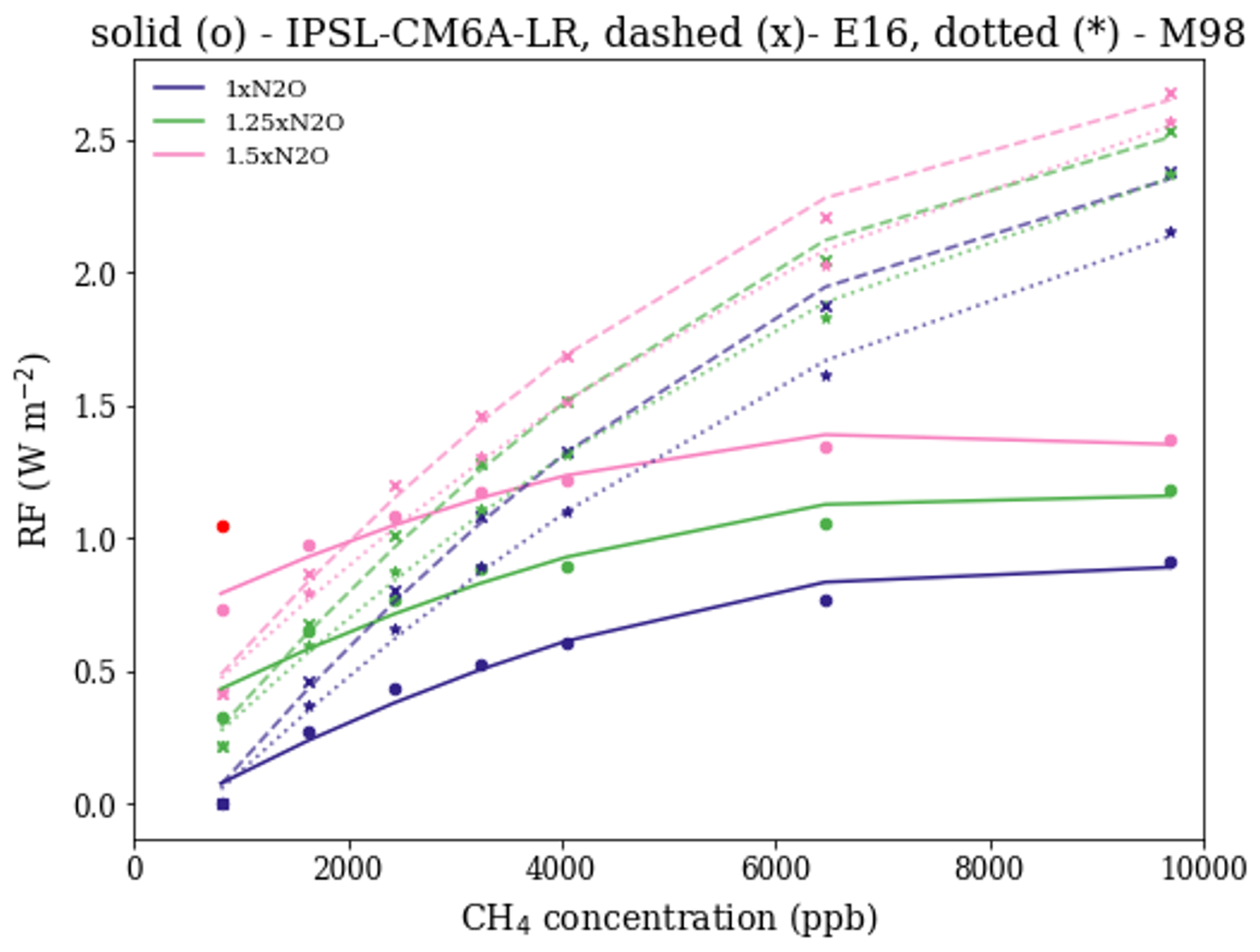
Figure A3 The ERF of CH₄ and N₂O from IPSL-CM6A-LR idealised experiments (points and fitted solid lines) and estimated from M98 (* and fitted dotted lines) and E16 (x and fitted dashed lines) equations, fitted to polynomial regressions for three levels of N₂O concentrations.

A system of equations can convert the input CH₄ and N₂O concentrations to the effective concentrations so that, if used in the climate model, they would yield actual forcing from the equations by E16. Among several linear and nonlinear functions to relate the actual concentrations of CH₄ and N₂O with the concentrations seen by the IPSL-CM6A model (effective concentrations) that have been tested, the following set of equations yielded the best fit:

$$\begin{array}{}\text{(A4)}& \begin{array}{rl}& {\mathrm{CH}}_{\mathrm{4}}^{\mathrm{effective}}={{\mathrm{CH}}_{\mathrm{4}}}_{t=\mathrm{0}}+a\times {\left({{\mathrm{CH}}_{\mathrm{4}}}^{\mathrm{actual}}-{{\mathrm{CH}}_{\mathrm{4}}}_{t=\mathrm{0}}\right)}^c\\ & {{\mathrm{N}}_{\mathrm{2}}\mathrm{O}}^{\mathrm{effective}}={{\mathrm{N}}_{\mathrm{2}}\mathrm{O}}_{t=\mathrm{0}}+b\times ({{\mathrm{N}}_{\mathrm{2}}\mathrm{O}}^{\mathrm{actual}}-{{\mathrm{N}}_{\mathrm{2}}\mathrm{O}}_{t=\mathrm{0}}{)}^d.\end{array}\end{array}$$

The initial values of CH₄ and N₂O concentrations are fixed at the preindustrial levels (t=0). Those of the effective CH₄ and N₂O concentrations are also assumed to take the same respective preindustrial levels. Eq. (A1) is used to relate the effective concentrations of CH₄ and N₂O of IPSL-CM6A-LR to the ERF estimated by E16:

$$\begin{array}{}\text{(A5)}& \begin{array}{rl}& {\mathrm{RF}}_{\mathrm{Etm}}={\mathrm{RF}}_{{\mathrm{CH}}_{\mathrm{4}},\mathrm{Etm}}+{\mathrm{RF}}_{\mathrm{N}\mathrm{2}\mathrm{O},\mathrm{Etm}}=\left(-\mathrm{1.3}\times {\mathrm{10}}^{-\mathrm{6}}\right.\\ & \times {\displaystyle \frac{\mathrm{1}}{\mathrm{2}}}\left({{\mathrm{CH}}_{\mathrm{4}}}^{\mathrm{effective}}+{{\mathrm{CH}}_{\mathrm{4}}}_{t=\mathrm{0}}\right)-\mathrm{8.2}\times {\mathrm{10}}^{-\mathrm{6}}\\ & \left.\times {\displaystyle \frac{\mathrm{1}}{\mathrm{2}}}\left({\mathrm{N}}_{\mathrm{2}}{\mathrm{O}}^{\mathrm{effective}}+{\mathrm{N}}_{\mathrm{2}}{\mathrm{O}}_{t=\mathrm{0}}\right)+\mathrm{0.043}\right)\\ & \times \left({\sqrt{{\mathrm{CH}}_{\mathrm{4}}}}^{\mathrm{effective}}-{\sqrt{{\mathrm{CH}}_{\mathrm{4}}}}_{t=\mathrm{0}}\right)+\left(\mathrm{4.2}\times {\mathrm{10}}^{-\mathrm{6}}\right.\\ & \times {\displaystyle \frac{\mathrm{1}}{\mathrm{2}}}\left({\mathrm{N}}_{\mathrm{2}}{\mathrm{O}}^{\mathrm{effective}}+{{\mathrm{N}}_{\mathrm{2}}\mathrm{O}}_{t=\mathrm{0}}\right)-\mathrm{4.9}\times {\mathrm{10}}^{-\mathrm{6}}\\ & \left.\times {\displaystyle \frac{\mathrm{1}}{\mathrm{2}}}\left({{\mathrm{CH}}_{\mathrm{4}}}^{\mathrm{effective}}+{{\mathrm{CH}}_{\mathrm{4}}}_{t=\mathrm{0}}\right)+\mathrm{0.117}\right)\\ & \times \left({\sqrt{{\mathrm{N}}_{\mathrm{2}}\mathrm{O}}}^{\mathrm{effective}}-{\sqrt{{\mathrm{N}}_{\mathrm{2}}\mathrm{O}}}_{t=\mathrm{0}}\right).\end{array}\end{array}$$

We optimise the four parameters of Eq. (A4) by minimising the sum of squared residuals between ERF estimated by E16 equations and simulated by IPSL-CM6A-LR using a Python implementation of the Limited-memory Broyden–Fletcher–Goldfarb–Shanno algorithm with bound constraints (L-BFGS-B), which is an algorithm for solving large nonlinear optimisation problems with simple bounds (Byrd et al., 1995). The cost function is defined as

$$\begin{array}{}\text{(A6)}& \mathrm{CF}={\sum }_i^{i=\mathrm{21}}{\left({\mathrm{RF}}_{\mathrm{IPSL}}-{\mathrm{RF}}_{\mathrm{Etm}}\right)}^{\mathrm{2}}.\end{array}$$

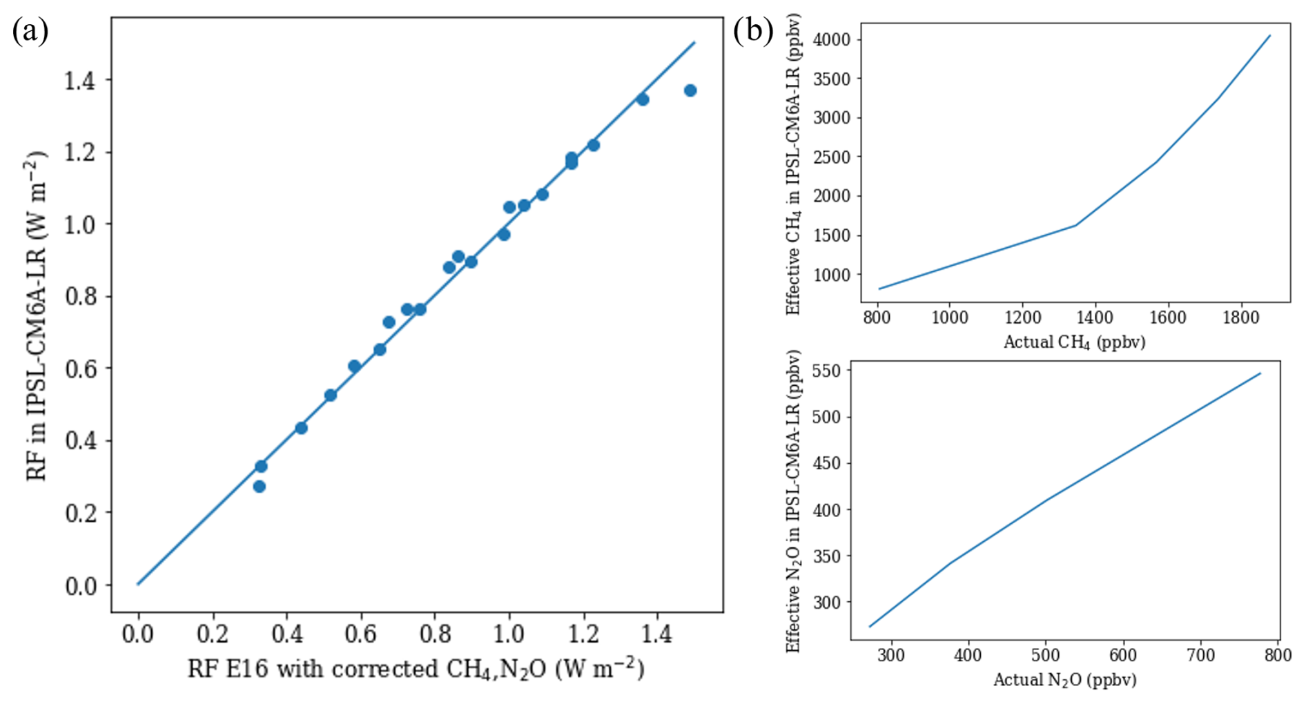
Figure A4 (a) Scatterplot of ERF simulated by IPSL-CM6A and estimated by E16 equations using the corrected effective concentrations from Eq. (A3) and (b) the effective IPSL-CM6A-LR concentrations of CH₄ and N₂O as a function of the actual concentrations derived via a system of nonlinear functions.

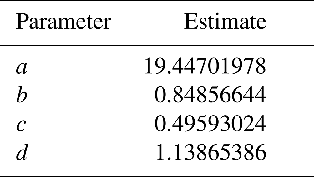
The residual error after fit equals 0.03 (W m⁻²)² (Fig. A4). The solution of the cost function provides the estimates of four uncertain parameters for Eq. (3), indicated in Table A2. The effective IPSL-CM6A-LR concentrations of CH₄ and N₂O are functions of the actual concentrations (Fig. A4b). Higher effective CH₄ and lower N₂O effective concentrations are needed for IPSL-CM6A-LR to reproduce the ERF in agreement with IPCC estimates.

Table A2 Estimated parameters in Eq. (A4).

The estimated parameters were applied to derive the effective IPSL-CM6A-LR concentrations for a target scenario (Fig. A5). Higher CH₄ and lower N₂O concentrations are required to reproduce the ERF correctly.

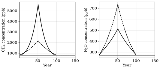
Figure A5 The actual (dashed lines) and new recalibrated effective CH₄ and N₂O IPSL-CM6A-LR concentrations (solid lines) for the CH₄–N₂O experiment of this study.