Dynamic vegetation highlights first-order climate feedbacks and their dependence on the climate mean state

We investigate how first-order albedo and water vapor radiative feedbacks are triggered by climate-vegetation interactions using mid-Holocene and pre-industrial climate simulations. The mid Holocene greening of the Sahara and northward shift of the northern tree line in the Northern Hemisphere illustrate these climate-vegetation interactions and challenge the development of Earth System models. We consider four different configurations for the IPSL Earth System model with dynamical vegetation to quantify vegetation and radiative feedbacks. They combine different parameterizations of key factors controlling vegetation functioning: bare soil evaporation, photosynthesis and associated parameters, and tree mortality. Whatever the model setup, the major differences between the mid-Holocene and pre-industrial climates are consistent with climate and vegetation reconstructions from pollen records. However, model setup differences modulate the way in which vegetation-climate interactions trigger first-order radiative surface albedo and water vapour feedbacks. Cascading effects involve both local snow-vegetation interactions and remote water vapour and long-wave radiative feedbacks. We show that the parameterization of bare soil evaporation is a key factor that controls tree growth in mid and high latitudes. Photosynthesis parameterization appears to be critical in controlling the seasonal evolution of the vegetation and leaf area index, as well as their effect on radiative feedbacks and the sensitivity of the vegetation feedback to the climate mean state. It even affects the sign of the global annual mean changes in temperature and precipitation between the mid-Holocene and pre-industrial periods. Dynamical vegetation highlights behaviours that can only be fully studied in a fully coupled Earth system model. The sensitivity of these vegetation-induced feedbacks to the mean climate state needs to be better considered when developing and tuning climate models.

1 Introduction

Climate-vegetation feedbacks are difficult to quantify because they depend on the mean climate state and, thereby, when it comes to simulations, to the characteristics of the simulated climate mean state that may differ from one model to another for the same climatic period (Braconnot and Kageyama, 2015). They are also hidden in the land surface albedo and atmospheric moisture radiative feedback in estimates of climate sensitivity (Sherwood et al., 2020). A reason for this is that vegetation lies at the critical zone between land and atmosphere. Its variations depend on interconnected factors such as light, energy, water and carbon, which in turn affect climate and environmental factors.

Paleoclimate simulations have provided evidence for the need to consider vegetation changes in climate change experiments. Typical examples concern the role of mid-latitude vegetation-snow albedo feedback first discussed for the last glacial inception, 115 000 years before present (Gallimore and Kutzbach, 1996; de Noblet et al., 1996). The combined response of temperature, snow and vegetation to the reduction of the summer insolation needs to be accounted for to simulate a glacial cooling in agreement with paleo reconstructions. Attempts to simulate the mid-Holocene green Sahara and northward shift of the tree line in the Northern Hemisphere 6000 years ago (i.e. Jolly et al., 1998; Prentice et al., 1996), have further revealed how vegetation affects land albedo, soil properties, and teleconnections (Claussen and Gayler, 1997; Joussaume et al., 1999; Levis et al., 2004; Pausata et al., 2017). The evidence for the need to better understand the role of dynamical vegetation in climate changes has also been provided when trying to reconcile the results of transient Holocene simulations with temperature reconstructions of the early Holocene (Dallmeyer et al., 2022; Liu et al., 2014; Marsicek et al., 2018; Thompson et al., 2022). Changes in vegetation are also key to understand the relationship between long-term changes in vegetation, external forcing and variability (Braconnot et al., 2019), as well as boreal forest tipping points (Dallmeyer et al., 2021).

However, despite the increase in model complexity and the growing number of models with a fully interactive carbon cycle, there are still only a few modelling groups using model configurations with fully interactive dynamic vegetation to investigate future climate change (see Fig. TS.2, Arias et al., 2021). Vegetation feedbacks are therefore overlooked when developing climate models or comparing simulations performed with different models, because the effect of the vegetation feedbacks is only partially interactive with climate when vegetation types are prescribed. There is thus a risk that the linkages between model results and model formulation of biophysical processes are not properly accounted for in model comparisons. A caveat is that dynamic vegetation introduces additional degrees of freedom in climate simulations. Consequently, a model that produces reasonable results when vegetation is prescribed may have poorer performance when changes in vegetation types are fully interactive with climate and carbon cycle (Braconnot et al., 2019).

Here we investigate the biophysical climate-vegetation interactions and the way they trigger first-order atmospheric radiative feedbacks at the top of the atmosphere in mid-Holocene and pre-industrial simulations. The mid-Holocene is a well-suited period for investigating feedbacks occurring at the seasonal time scale and changes in the hydrological cycle (Braconnot et al., 2012; Joussaume and Taylor, 1995). At that time, the Earth's orbital configuration was such that the incoming solar radiation at the top of the atmosphere was larger in high latitudes and smaller in the tropics, and its seasonality was enhanced in the Northern Hemisphere and reduced in the Southern Hemisphere (Joussaume and Taylor, 1995; Kageyama et al., 2018; Otto-Bliesner et al., 2017). The mid-Holocene is a reference period of the Paleoclimate Modelling Intercomparison Project (PMIP), and vegetation feedback has been a focus of PMIP since its early days (Joussaume and Taylor, 1995). The aim has been to either understand vegetation changes and feedback on climate (i.e. Claussen and Gayler, 1997; Texier et al., 1997) and to evaluate model results (i.e. Harrison et al., 1998, 2014). Holocene simulations with dynamic vegetation still have large model biases in the representation of vegetation, such as an underestimation of the mid-Holocene green Sahara (Pausata et al., 2020). Some of the difficulties arise from differences in the vegetation and land surface models (Hopcroft et al., 2017). Previous climate simulations of the mid-Holocene also emphasised the role of indirect feedbacks of the vegetation on ocean circulation or sea-ice, amplifying or damping the direct effect of vegetation on climate (Gallimore et al., 2005; Otto et al., 2009b; Wohlfahrt et al., 2004). The results of these simulations raised concerns about the strength of the forest-snow albedo feedback affecting the temperature signal in spring, suggesting that ocean-sea-ice feedbacks could have a dominant climate impact (Otto et al., 2011).

The starting point of this study comes from difficulties in representing boreal forests in the IPSLCM6-LR standard version of the IPSL climate model (Boucher et al., 2020), and the fact that unavoidable and still poorly understood feedbacks resulting from vegetation-climate interactions and radiative feedbacks control the model results in the fully coupled system. Our objectives are thus to both improve the understanding of the first-order cascading climate-vegetation feedbacks in the fully coupled system, and identify their dependence on the land surface model representation of key processes affecting plant hydrology or leaf area index development. Indeed, the climate- vegetation feedbacks have a direct effect on temperature, controlling vegetation, leaf area index, productivity, evapotranspiration, soil moisture, as well as snow and ice cover. These interconnections make it difficult to determine the exact factors affecting the representation of vegetation in a fully interactive model. Starting from IPSLCM6-LR (Boucher et al., 2020), we developed four different settings of the land surface model by combining differences in the choice of the parameterisation of key factors known to affect the functioning of vegetation: photosynthesis, bare soil evaporation, and parameters defining the vegetation competition and distribution. We first compare the mid-Holocene climate changes obtained using the different model versions. We focus on estimating the atmospheric radiative feedbacks resulting from surface albedo, atmospheric water content, and lapse rate, following Braconnot and Kageyama (2015). We analyse the dependency of these first-order feedbacks on the mid-Holocene vegetation changes. We also focus on the differences in these feedbacks between the model versions, considering the mid-Holocene and the pre-industrial climates separately, so as to understand the dependence of the seasonal vegetation and radiative feedbacks on the climate mean state. We adapted the simplified conceptual framework that has been developed to quantify shortwave radiative feedbacks between two periods (Taylor et al., 2007) to the analyses of the radiative feedback between model versions. To do this, we assume that analysing differences in radiative feedbacks between two model versions is equivalent to analysing radiative feedbacks between two climatic periods.

The remainder of the manuscript is organized as follows: Section 2 presents the set-up of the four model configurations and the suite of experiments. Section 3 is dedicated to the analyses of the differences between the mid-Holocene and the pre-industrial climates, including the quantification of the atmospheric feedbacks resulting from the climate's response to the mid-Holocene insolation forcing. Section 4 goes deeper into the analyses of these feedbacks, considering the differences between the mid-Holocene simulations and making the linkages between these differences and the model content. It then addresses the question of the feedback dependence on the mean climate state. Section 5 provides an overall synthesis, and discusses the role of the photosynthesis parameterisation, as well as the implications of this study for model evaluation and carbon sources and sinks. The conclusion is in Sect. 6.

2 Model and experiments

2.1 IPSL model and different settings of the land surface component ORCHIDEE

The reference IPSL Earth climate model version for this study is IPSLCM6-LR (Boucher et al., 2020). This model version has been used to produce the suite of CMIP6 experiments (Eyring et al., 2016), including the mid-Holocene PMIP4-CMIP6 (Braconnot et al., 2021). The atmospheric component LMDZ (Hourdin et al., 2020) has a regular horizontal grid with 144 points in longitude and 142 points in latitude (2.5°×1.3°). This version of the model has 79 vertical layers extending up to 80 km. The land surface component ORCHIDEE version v2.0 operates on the atmospheric resolution. It includes 11 vertical hydrology layers and 15 plant functional types (Cheruy et al., 2020). The ocean component NEMO (Madec, Gurvan et al., 2017) uses the eORCA 1° nominal resolution and 75 vertical levels. The sea ice dynamics and thermodynamics component NEMO-LIM3 (Rousset et al., 2015; Vancoppenolle et al., 2009) and the ocean biogeochemistry component NEMO-PICES (Aumont et al., 2015) are run at the ocean resolution. The oceanic and atmospheric components are coupled via the OASIS3-MCT coupler (Craig et al., 2017) with a time step of 90 min.

Compared to the PMIP4-CMIP6 mid-Holocene simulations (Braconnot et al., 2021), the dynamical vegetation module (Krinner et al., 2005) is switched on for all the simulations included in this study. The vegetation dynamics is based on the approach of the LPJ model (Sitch et al., 2003). It computes the evolution of the vegetation cover in response to climate. It accounts for several climate constraints (e.g., minimum and maximum temperature) that affect vegetation fitness and competition between plant functional types (PFTs) based on their relative productivity.

Starting from this reference version, two formulations of bare soil evaporation and photosynthesis have been tested. The test made on bare soil evaporation uses developments that are described in detail in the ORCHIDEE hydrology documentation by Ducharne et al. (2018). In the standard version of the IPSLCM6-LR model, bare soil evaporation depends on the moisture content of the first 4 of the 11 soil layers (Milly, 1992). The bare soil evaporation rate corresponds to the potential evaporation rate when the moisture supply meets the demand (Cheruy et al., 2020). Another solution has been developed to better represent soil evaporation processes, by considering the ratio (mc) between the moisture in the litter zone (the first four surface layers) and the corresponding moisture at saturation (Sellers et al., 1992). With this parameterization, the aerodynamic resistance is decreased by a factor $\mathrm{1}/\text{rsoil}$, where:

$$\begin{array}{}\text{(1)}& \text{rsoil}={\mathrm{e}}^{\mathrm{8.206}-\mathrm{4.255}\times \mathit{mc}}\end{array}$$

This adjustment in the bare soil evaporation parameterization was not incorporated into IPSLCM6A-LR due to the fact that it induces a surface warming that was not fully understood (Cheruy et al., 2020). For simplicity, the two parameterisations are respectively referred to as bareold and barenew in the following (Table 1). Note that, even though this change resembles the one discussed in Hoptcroft and Valdes (2021), it is different since we only consider bare soil evaporation here and not the whole evapotranspiration.

Table 1 Characteristics of the different simulations. The columns refer to the simulation names, the initial state, and the length of the mid-Holocene (MH) and pre-industrial (PI) simulations. We provide the names used in this paper, as well as our internal simulation numbers in brackets. Only the initial state of the ocean-ice-atmosphere component is provided, since all simulations except V4 PI start from bare soil.

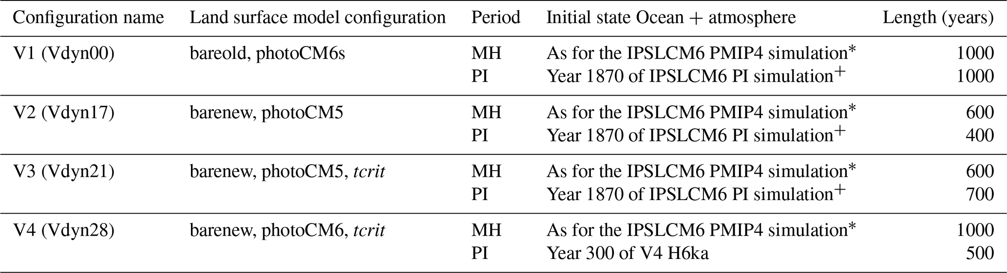
^∗ See Braconnot et al. (2021), ⁺ see Boucher et al. (2020).

The parameterization of photosynthesis/stomatal conductance used in the ORCHIDEE land surface model (Fig. 1) differs between IPSLCM5A-LR (Dufresne et al., 2013) and IPSLCM6-LR (Boucher et al., 2020). In IPSLCM5A-LR (Fig. 1), the photosynthesis (PhotoCM5) is represented by the standard Farquhar model for C3 plants (Farquhar et al., 1980) which has been extended to C4 plants (Collatz et al., 1992) and coupled to the Ball and Berry stomatal conductance formulation (Ball et al., 1987). In IPSLCM6-LR (Fig. 1), the photosynthesis/conductance (PhotoCM6) has been improved to include the approach based on Yin and Struik (2009) coupled to the original Farqhuar (1980) model. The PhotoCM6 parameterization benefits from an explicit solving of the coupled photosynthesis/stomatal conductance, providing a more accurate solution than the previous iterative resolution. Important differences between the two approaches are due to the fact that stomatal conductance is driven by the vapor pressure deficit in PhotoCM6, whereas in PhotoCM5 it is based on relative humidity. Also, the shape of the response of the photosynthesis to temperature is different (Fig. 1). The temperature response is a bell-shape function in PhotoCM5. It is possible to control the minimum, maximum and optimal temperatures of photosynthesis independently of the maximum photosynthesis rate. The response of photosynthesis to temperature is driven by a modified Arrhenius function in PhotoCM6, with a reference temperature of 25 °C. Hence, the fixed maximum rate of carboxylation Vcmax is the rate at 25 °C, whereas it is the optimal Vcmax in PhotoCM5 (Fig. 1), and the parameters (named ASJ) of the Arrhenius function are prescribed. The temperature response cannot be fully controlled, which is why we reimplemented the PhotoCM5 parameterisation to run our tests with IPSLCM6-LR. Another important difference is that, in PhotoCM6, the response to temperature is adapted to the local long-term (i.e., 10 years) temperature of each pixel, which is not the case for PhotoCM5.

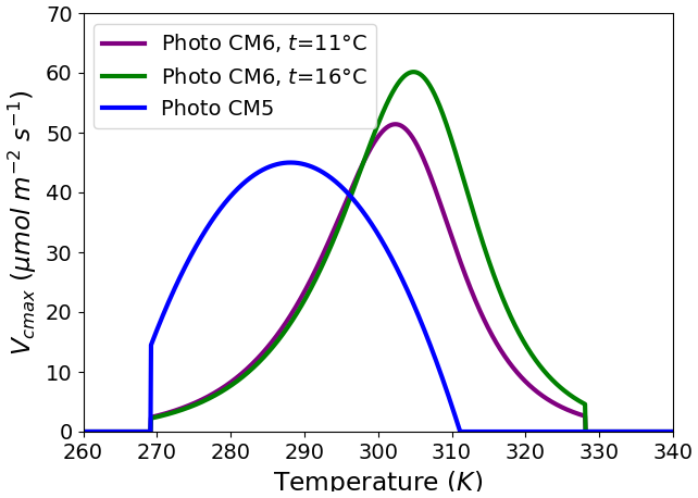
Figure 1 Maximum rate of carboxylation (Vcmax, $\mathrm{mmol}{\mathrm{m}}^{-\mathrm{2}}{\mathrm{s}}^{-\mathrm{2}}$) as a function of surface air temperature (K) for the two photosynthesis parameterizations (photoCM5 and photoCM6) and PFT 7 (Boreal Needleleaf Evergreen). As photosynthesis depends on the long term mean monthly temperature, the Vcmax curves are plotted for mean temperatures of 11 and 16 °C. Note that with the choice we made, Vcmax at 25 °C for photoCM6 and the maximum value of photoCM5 are the same. See the text for details on the parameterizations.

These differences in the shape of the function have some implications for some of the adjustments we made to the original parameterisations to compensate for the tendency of the climate model to be too cold in some mid-to-high-latitude regions (Boucher et al., 2020). The objective was to allow photosynthesis at lower temperatures. The parameters of photoCM6 have been adjusted using offline simulations forced by atmospheric reanalysis. The objective was to find optimal limits in temperature for PhotoCM6 and to adjust Vcmax at 25 °C and ASJ within an acceptable range of values. In the standard version of the IPSLCM6-LR model, these parameters are the standard ones, and we add a “s” to the name in that case (Table 1). The photoCM5 parameterisation uses the standard values of PhotoCM6. The two parameterizations account for the effect of atmospheric CO2 concentration. This effect impacts both the rate of photosynthesis and stomatal conductance. There is no difference in formulation between PhotoCM5 and PhotoCM6, but differences arise from the interaction with the effect of the other changes we made.

Another important process determining the possibility for forest to grow in a cold environment is the critical temperature for tree regeneration (tcrit). Indeed, it is assumed that, even for boreal forest, very low winter temperatures result in insufficient fitness for reproduction and then forest regeneration. In the standard model version, the critical temperature is −45 °C for Boreal Needleleaf Evergreen (PFT 7) and Boreal Broadleaf Summergreen (PFT 8). It means that when the daily temperature falls below 45 °C a fraction of trees dies. This threshold was too high, given that regions covered by boreal forests regularly experience temperatures below −45 °C in current climate conditions. We therefore changed the critical temperature to −60 °C, the standard value used for Larix (PFT 9). We took the risk of simulating a wrong composition of boreal forest.

2.2 Experiments

We consider a set of four experiments (Table 1). For each of them, we performed a mid-Holocene simulation following the PMIP4-CMIP6 protocol (Otto-Bliesner et al., 2017) as in Braconnot et al. (2021), and a pre-industrial CMIP6 simulation (Eyring et al., 2016). In this study, the pre-industrial climate has a similar Earth's orbital configuration to that of today, with the summer solstice occurring at the perihelion and the winter solstice at the aphelion. These experiments represent key steps in a wider range of tests designed to improve the representation of boreal forest. Model developments were done using the mid-Holocene as a reference for natural vegetation, knowing that the pre-industrial climate is affected by land use, which is not considered in these experiments. Our approach provides a paleo constraint on the choice of model set up for climate change experiments (e.g. Hopcroft and Valdes, 2021).

The different model setups for these simulations are listed in Table 1. The first experiment, V1, is performed with the standard model version and the dynamic vegetation switched on. The differences with the simulations presented in Braconnot et al. (2021) are only due to the dynamical vegetation-climate interactions. All the other experiments include the new parameterization of bare soil. Experiments V2 and V3 have the PhotoCM5 parameterisation of photosynthesis. In V3, the critical temperature is modified for boreal forests. The final version, V4, is similar to V3, but it uses PhotoCM6 photosynthesis. Note also that some bugs and inconsistent choices when running with or without the dynamical vegetation have been found in the standard model version V1. They have been corrected for the sensitivity tests and do not affect the results, which only focus on key factors that have emerged from a large suite of shorter systematic sensitivity experiments. Version V4 is considered as the reference version for ongoing Holocene transient simulation with dynamic vegetation.

The initial state for all the simulations corresponds to a restart of the IPSLCM6-LR model for the ocean–atmosphere-sea-ice-icesheet system. The land-surface model starts from bare soil. We follow here the protocol used by Braconnot et al. (2019). We tested that, as in our previous set of Holocene experiments with dynamical vegetation (see Braconnot et al., 2019), the results would be the same when an initial state for the land surface model with dynamical vegetation (and not only the vegetation map) from a previous simulation is used as the initial state. This is mainly due to the fact that the land surface covers only ∼30 % of the Earth's surface and does not store energy on a long-timescale, unlike the ocean. The initial state corresponds to a mid-Holocene or PI climate depending on the simulated period, except for the pre-industrial simulation using V4, for which the initial state is from the mid-Holocene simulation (Table 1).

2.3 Vegetation-climate adjustments to incoming solar radiation and atmospheric composition

A similar sequence is found for the vegetation adjustment time in all experiments (Fig. 2). Starting from bare soil imposes a cold start for the land surface, since bare soil has a larger albedo than grass or forest. It is characterized by a negative heat budget at the surface (Fig. 2b), a colder 2 m air temperature (Fig. 2c), reduced precipitation and atmospheric water content (Fig. 2d and e), an increase in sea ice volume (Fig. 2f), a reduced ocean surface heat content (Fig. 2h), a large albedo (Fig. 2i) and soil moisture (Fig. 2j). There is a rapid adjustment due to the fact that snow cover is also absent in the initial state, so that it doesn't amplify the initial cooling. In each of the simulations, the first 50 years are characterised by rapid vegetation growth, with the well-known succession of grass and trees also discussed in Braconnot et al. (2019). This first rapid phase is followed by a long-term adjustment related to slow climate-vegetation feedback of about 300 years. As expected, the ocean heat content adjustment has the largest adjustment time scale. The equilibrium state is characterized by multiscale variability. This interannual to multidecadal variability is smaller than the differences between the experiments but needs to be accounted for in order to properly discuss differences in the simulated climatology.

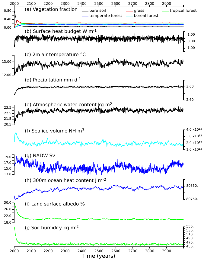
Figure 2 Adjustment time for the global average of the simulated V4 mid-Holocene vegetation, and a subset of atmosphere (black), sea-ice (light blue), ocean (blue) and land (green) variables. The different panels represent respectively (a) the coverage (fraction) of 4 major vegetation types (grass, tropical forest, temperate forest, and boreal forest) and bare soil, (b) the surface heat budget (W m⁻²), (c) the 2 m air temperature (°C), (d) the precipitation (mm d⁻¹), (e) the atmospheric water content (kg m⁻²), (f) the sea ice volume (m³) in the Northern Hemisphere (NH), (g) the North Atlantic Deep Water (NADW, Sv), (h) the surface to 300 m depth ocean heat content (J m⁻²), (i) the land surface albedo (%) and (j) the soil humidity (kg m⁻³).

A conclusion from Fig. 2 is that 300 years of simulation is a minimum for analysing the difference between the simulations, which is consistent with the adjustment time reported by Braconnot et al. (2019). It justifies our choice to save computing time by considering simulation lengths ranging from 400–1000 years depending on the experiment (Table 1).

3 Simulated changes between mid-Holocene and pre-industrial climates

3.1 Temperature and precipitation changes

We first focus on the mid-Holocene changes simulated by the four versions of the model, using the simulated pre-industrial climate as a reference. The major differences between the model versions are well depicted in Fig. 3 considering only annual mean surface air temperature and precipitation for the V3 and V4 model versions. During mid-Holocene, the larger tilt of the Earth's axis induces a slight reduction in incoming solar radiation in the tropics and an increase in high latitudes. This effect is further amplified (or dampened) by the fact that, during the mid-Holocene, Earth's precession enhances the insolation seasonality in the Northern Hemisphere and decreases it in the Southern Hemisphere (COHMAP-Members, 1988). Thus, the annual mean reflects both the annual mean change in insolation and the associated atmospheric, oceanic and land surface seasonal feedbacks. It is characterised by an annual mean warming in mid and high latitudes in the Northern Hemisphere and an annual mean cooling in the Southern Hemisphere (Fig. 3). The annual mean cooling in the tropics over land is a fingerprint of the enhanced boreal summer monsoon (Joussaume et al., 1999). The latter is driven by dynamical effects that deplete precipitation over the ocean and increase it over land (Braconnot et al., 2007; D'Agostino et al., 2019). These results are consistent with those of the multimodel ensemble of PMIP mid-Holocene simulations (Brierley et al., 2020). They cover a large fraction of the spread of temperature changes produced by different models worldwide (Brierley et al., 2020), and stress that cascading feedbacks induced by dynamic vegetation have a profound impact on regional climate characteristics.

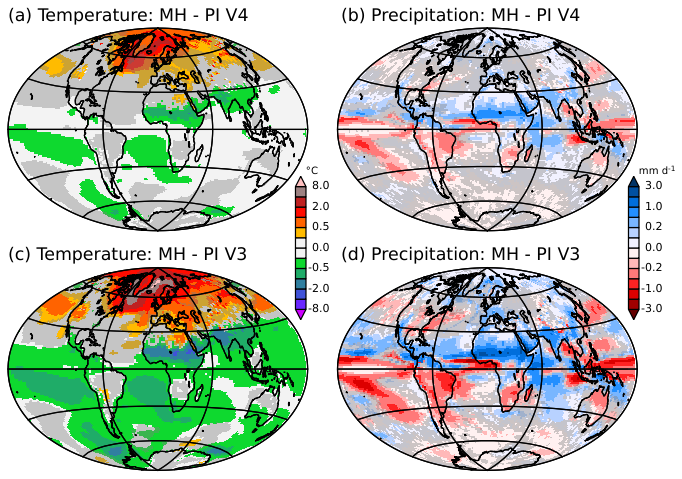
Figure 3 Simulated mid-Holocene (MH) minus Preindustrial (PI) differences for (a) and (c) the 2 m air temperature (°C) and (b) and (d) the precipitation (mm d⁻¹) and (a) and (b) the V3 and (c) and (d) V4 model versions. Changes are considered to significant at the 5 % level outside the grey zones. The significance is estimated from all combinations of differences in 100-year averages between MH and PI simulations. For these estimates the first 300 years of the simulations are excluded.

The results of the different model versions are compared in Fig. 4 to those of the PMIP4 mid-Holocene simulations discussed in Braconnot et al. (2021) and the climate reconstructions from pollen and macrofossils data by Bartlein et al. (2011). The model results have been first interpolated to the 1°×1° grid of the climate reconstruction. Within each region, the regional average only considers grid points for which a value is available in the reconstruction. The spread between these different 100 years differences for a given model version highlights the fact that long-term variability introduces uncertainties in 100 years estimates of about 0.5–3 °C depending on the region (Fig. 4). Uncertainties resulting from long term variability need to be accounted for since 100 years variability can be as high as the signal in some places. This has been discussed for a long time for paleoclimate simulations (Hewitt and Mitchell, 1996; Otto et al., 2009a), but modelling groups still tend to only provide simulations with limited length when contributing to the PMIP database for model intercomparisons (Brierley et al., 2020). Neglecting this long-term variability can lead to erroneous model ranking or interpretation of model differences. Centennial variability is significant here, but the major differences between the simulations are robust.

The Fig. 4 completes the maps presented in Fig. 3 by indicating that the largest annual mean warming in mid and high latitudes is found for V2, and that for most of the boxes V2 simulated changes in temperature and precipitation are not statistically different from those simulated with V3 when accounting for variability between 100 year averages. All versions with dynamic vegetation produce larger changes in West Africa than the IPSL PMIP4 simulations for which the vegetation was fixed to the pre-industrial values. This result is expected from vegetation feedback (Braconnot et al., 1999). The total amount is however still not as large as the one expected from the reconstruction. In most boxes, it is still difficult to have the different variables for a given model version in agreement with the reconstructions in all regions despite their large error bars (Fig. 4). An interesting case is Eurasia, a region where reconstructions indicate more precipitation during the mid-Holocene and most models simulate a decrease, which has been attributed to a lack of eastward penetration of the westerlies (Bartlein et al., 2017). Only versions V2 and V3 agree with this increase in precipitation. The results obtained with version V4 appear to be in overall better agreement with climate reconstructions than results obtained with the other model versions. They are the closest to those obtained for the PMIP4 mid-Holocene simulations using the standard IPSLCM6 model version.

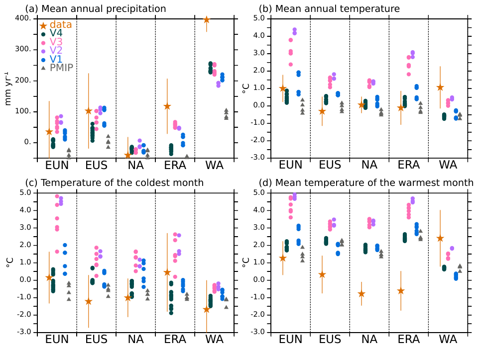
Figure 4 Comparison of the simulated Mid-Holocene (MH) minus Pre-industrial (PI) differences with Bartlein et al. (2011) reconstructions for (a) the mean annual precipitation (mm yr⁻¹), (b) the mean annual temperature (°C), (c) the temperature of the coldest month (°C) and (d) the temperature of the warmest month (°C) and 5 selected regions with high data coverage: Northern Europe (EUN), Southern Europe (EUS), North America (NA), Eurasia (ERA) and West Africa (WA). A mask is applied to consider only the grid points with values in the reconstruction on the common 1°×1° reconstruction grid chosen for this comparison. The uncertainty bars for the reconstruction are estimated from the uncertainties provided in Bartlein et al. (2011) files. For each tmodels, each dot corresponds to a cross 100 year mean difference between MH and PI simulations (see text).

3.2 Land surface feedbacks between mid-Holocene and pre-industrial climates

The differences in the mid-Holocene simulated changes between the model versions come from the various vegetation and radiative feedbacks induced by the different changes in the land-surface. We computed the mean root mean square difference between the two climates for leaf area index (LAI), snow, and atmospheric water content (Fig. 5). This measure allows us to account for both the differences in the annual mean and in seasonality, since the monthly differences between the mid-Holocene and pre-industrial periods have different signs depending on the season. In order to also account for the centennial variability, we use all possible combinations of 100 years annual mean cycle differences between the two periods for these rms estimates, neglecting the first 300 years of each simulation. For a given variable var in simulation 1 (var1) and simulation 2 (var2) the rms is thus computed as:

$$\begin{array}{}\text{(2)}& \text{rms}\left(\text{var}\right)=\sqrt{{\displaystyle \frac{\mathrm{1}}{n_{\mathrm{1}}\times n_{\mathrm{2}}}}\sum _{i=\mathrm{4}}^{n_{\mathrm{1}}}\sum _{j=\mathrm{4},j\ge i}^{n_{\mathrm{2}}}\sum _{m=\mathrm{1}}^{\mathrm{12}}(\mathit{\text{var1}}-\mathit{\text{var2}}{)}^{\mathrm{2}}}\end{array}$$

where n₁ and n₂ represent the number of non-overlapping 100 years periods in simulation 1 and 2, respectively (and neglecting $n=\mathrm{1}-\mathrm{3}$ for the first 300 years), and m refers to months, with 1 being the first month of the year and 12 the last month. The dispersion between the 100 year estimates provides a measure of the uncertainty.

The LAI rms between mid-Holocene and pre-industrial climates (Fig. 5a–d) highlights a simulated change in vegetation (LAI) in almost all regions at the mid-Holocene compared to the pre-industrial period. This is found with all four model versions. It also shows that regions experiencing the largest changes are the Sahel, the Sahara, northern India, Eurasia and the eastern part of North America, although the magnitude and regional details depend on the model version. The large LAI changes in Africa highlight that all of these model versions produce a green Sahara which was not the case with the previous versions of the IPSL model (Braconnot et al., 2019). This is consistent with the increase in annual mean precipitation and the decrease in temperature (Fig. 3). Large vegetation changes are simulated even though the annual mean precipitation seems to be underestimated (Fig. 4). Note that this large amplification couldn't be anticipated from the standard PMIP4-CMIP6 simulation where vegetation is prescribed to pre-industrial vegetation, even though changes in monsoon rainfall were larger than in previous IPSL model versions (Braconnot et al., 2021).

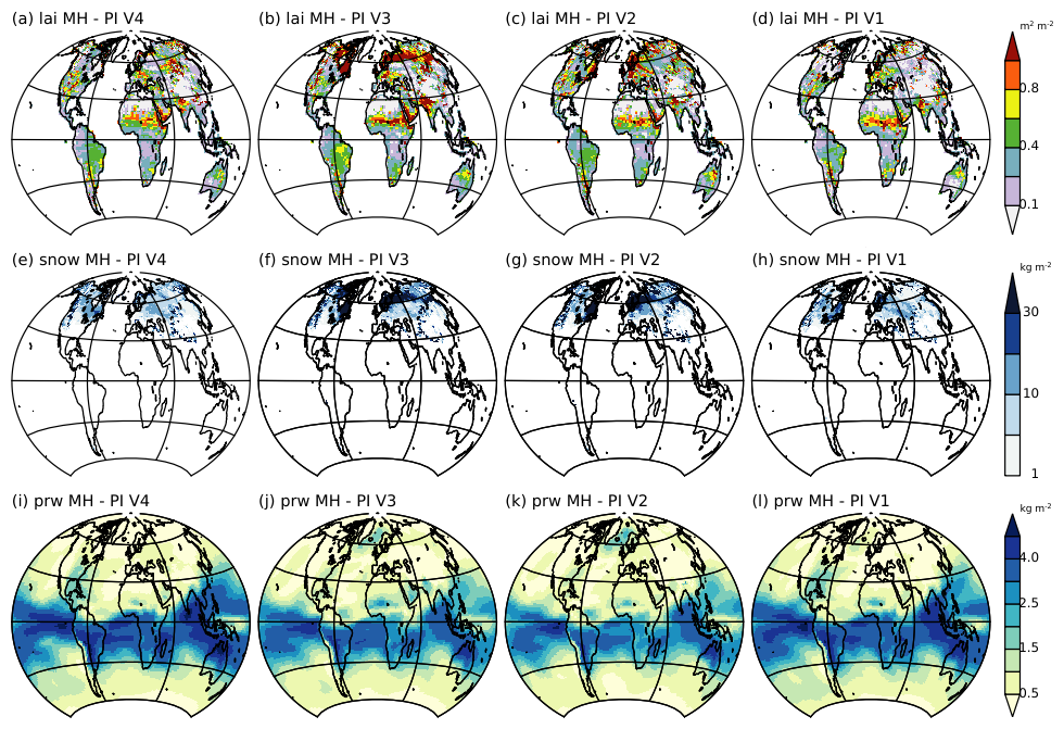
Figure 5 Root mean square difference between Mid-Holocene (MH) and Pre-industrial (PI) climates calculated by considering all combinations of 100 year annual mean cycles between the two periods at each grid points for (a–d) LAI, (d–h) the snow mass (kg m⁻²), and (i–l) the atmospheric water content (kg m⁻²). Note that for snow mass the estimates have been restricted to 100 years monthly differences between February and May, which corresponds to the period where snow feedback over Eurasia is the largest between these two periods.

The model versions producing the largest annual mean temperature changes in Eurasia and eastern North America are also those (V2 and V3) producing the largest changes in LAI (Fig. 5). The snow rms indicates that these regions coincide with those experiencing the largest changes in snow cover (reduced snow cover during the mid-Holocene). These regional interlinkages between the different variables are more pronounced for the two model versions (V2 and V3) with the largest temperature changes (Figs. 3 and 4). It is the footprint of a direct feedback loop between vegetation, temperature and snow cover, which further triggers temperature changes through the surface albedo feedback. The mid-Holocene forcing and the response of temperature, snow, and sea-ice also induce substantial differences in the atmospheric water content (Fig. 5). The two model versions (V2 and V3) with the largest temperature changes in high latitudes produce the largest changes in sea ice between the two periods, and thereby in water vapor in the north Atlantic (Fig. 5 right (i–l), right column). In the tropics, where water vapour changes are large for all model versions, the largest values are found for the other two versions, V1 and V4 (Fig. 5).

3.3 Estimations of the radiative feedbacks between mid-Holocene and pre-industrial climates

We further estimate the radiative feedbacks (Fig. 6). We quantify the shortwave (SW) radiative impact of surface albedo (α_s), atmospheric absorption (μ) and scattering (γ) on the Earth's radiative budget at the top of the atmosphere using the simplified method developed by Taylor et al. (2007). It consists of estimating the integral properties of the atmosphere (e.g. absorption and scattering) and the effect of the surface albedo on the shortwave radiative flux at the top of the atmosphere. Following Braconnot et al. (2021), we first estimate for each simulation the atmospheric absorption μ as:

$$\begin{array}{}\text{(3)}& \mathit{\mu }={\mathit{\alpha }}_{\mathrm{p}}+\left({\displaystyle \frac{{\text{SW}}_{\text{si}}}{{\text{SW}}_{\mathrm{i}}}}\right)(\mathrm{1}-{\mathit{\alpha }}_{\mathrm{p}}),\end{array}$$

and the atmospheric scattering γ as:

$$\begin{array}{}\text{(4)}& \mathit{\gamma }={\displaystyle \frac{\mathit{\mu }-({\text{SW}}_{\text{si}}/{\text{SW}}_{\mathrm{i}})}{\mathit{\mu }-{\mathit{\alpha }}_{\mathrm{s}}({\text{SW}}_{\text{si}}/{\text{SW}}_{\mathrm{i}})}},\end{array}$$

where SW_i and SW_si stand respectively for the incoming solar radiation at the top of the atmosphere (insolation) and at the surface, and α_p for the planetary albedo. The planetary and surface albedos are computed from the downward and upward SW radiations. By replacing the factors obtained for one climate (or one simulation) one by one with those obtained for the other climate (or another simulation), we can access to the radiative effect of this factor between the two climates (or two simulations). As an example, using simulation 1 as the reference, the effect of a change in the surface albedo in simulation 2 compared to simulation 1 is provided by:

$$\begin{array}{}\text{(5)}& {\mathit{\alpha }}_{\mathrm{p}}({\mathit{\mu }}_{\mathrm{1}},{\mathit{\gamma }}_{\mathrm{1}},{\mathit{\alpha }}_{{\mathrm{s}}_{\mathrm{2}}})-{\mathit{\alpha }}_{\mathrm{p}}({\mathit{\mu }}_{\mathrm{1}},{\mathit{\gamma }}_{\mathrm{1}},{\mathit{\alpha }}_{{\mathrm{s}}_{\mathrm{1}}})\end{array}$$

The decomposition done for short wave radiation is not valid for long wave (LW) radiation (Taylor et al., 2007). However, in the case of the simulations considered here, we can assume that the LW forcing due to trace gases is small (Braconnot et al., 2012; Otto-Bliesner et al., 2017). The mid-Holocene change in outgoing longwave radiation at the top of the atmosphere (TOA) thus corresponds to the total LW radiative feedbacks. The outgoing long wave at TOA is composed of two terms: the surface outgoing longwave radiation (LW_sup∼σT⁴, where σ is the Stefan–Boltzmann constant) induced by the surface temperature and the atmospheric heat gain (LW_sup−LW_TOA) resulting from the combination of changes in atmospheric water vapor, clouds and lapse rate. The relative magnitude of these three terms cannot be estimated here.

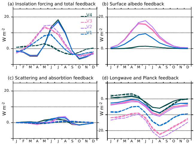
Figure 6 Radiative forcing and feedbacks estimated at the top of the atmosphere (W m⁻²) between the mid-Holocene and the pre-industrial climates over the mid-to high latitudes in the Northern Hemisphere (45–80° N) for the four model versions. (a) Radiative forcing (solid lines) and total radiative feedbacks (dash lines), (b) surface albedo feedback, (c) atmospheric scattering (solid lines) and absorption (dash lines) feedbacks, and (d) longwave feedback (solid line) and Planck response (dash lines). The colours of the different curves correspond to the model version.

For this feedback quantification, we focus on the mid to high latitudes between 45 and 80° N where the differences in LAI and in snow cover between the mid-Holocene and the pre-industrial simulations are the largest (Fig. 6). The V2 and V3 versions of the model produce a total radiative feedback as large as the forcing, except that the feedback is maximum in boreal spring, whereas the forcing is maximum in summer and early autumn. The dominant feedback factor is the land surface albedo (Fig. 6b). It results from the combination of vegetation and snow cover changes, with a dominant effect of snow albedo. The snow albedo effect is the largest for grid points where grass is replaced by forest in the mid-Holocene simulation, which occurs over a large area in Eurasia in V2 and V3 compared to V1. The effect is more muted in V1 because grass is dominant in both periods, or in V4 because a larger fraction of forest compared to the other simulations is still present in the pre-industrial simulation (Fig. 7). Feedbacks in LW radiation also have a significant impact on modifying the top of the atmosphere's total radiative fluxes. It reduces the effect of the albedo feedback by allowing more heat to escape to space, with maximum effect from June to October (Fig. 6d). Interestingly, the direct surface temperature effect (Planck) is partly compensated by an increased greenhouse gas effect resulting from increased water vapor and change in atmospheric lapse rate, in places where the surface warming is maximum (Figs. 3 and 5).

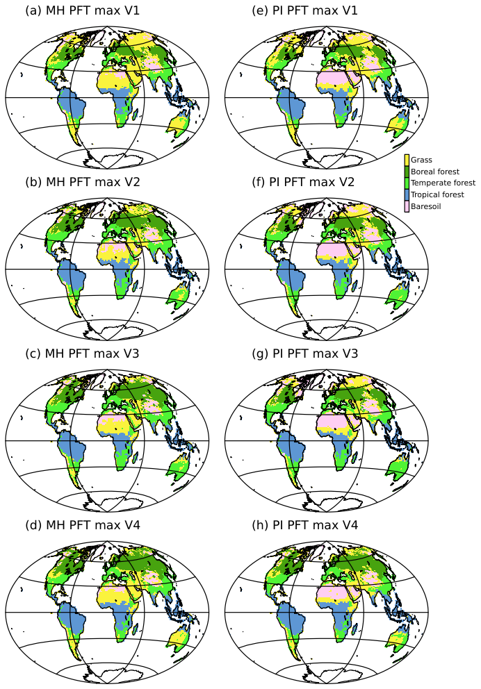
Figure 7 Dominant type of vegetation (PFT MAX) as simulations by the four model versions for (a–d) the mid-Holocene (MH) and (d–f) the pre-industrial (PI) climates. For clarity the 15 plant functional types (PFTs) have been grouped into 5 major vegetation types: 1. Bare soil, 2. Tropical forest, 3. Temperate forest, 4. Boreal forest, and 5. Grass. These maps represent the vegetation average over the length of the simulation, without considering the first 300 years.

4 Differences between model versions and dependence of radiative feedbacks on climate mean state

The first-order feedbacks between vegetation, temperature, snow, and albedo highlighted in the previous section have different magnitudes depending on the model versions (Fig. 6). This arises from differences in model land surface parameterisation and first-order albedo and water vapor feedbacks, some of which may mask the effect due to land surface parameterisation. We thus investigate if we can attribute some of the systematic differences in climate and vegetation cover to the different parameterizations and tuning we made.

4.1 Systematic differences between model versions for the mid-Holocene

The successive model developments were targeted at producing mid-Holocene boreal forest as the dominant type of vegetation further north in Eurasia and North America when going from the V1 to the V4 versions of the model (Fig. 7). We present the global vegetation assemblages of the 15 PFTs in Fig. 8. This figure complements Fig. 7, where only the dominant type of vegetation is presented in each model grid box. The global averages in Fig. 8 reflect the major differences found at the regional scale. As expected from model developments, major differences between the mid-Holocene simulations are found for boreal forest, and in particular Boreal Needleleaf Evergreen (PFT 7) (Fig. 8a). This PFT represents about 5 %–10 % of the total vegetation cover in V1 and V2, and 13 % in V3 and V4. In V2, Boreal Needleleaf Deciduous (PFT 9) is the dominant type of boreal forest, representing 9 % of the total vegetation cover. This simulation doesn't include the change in tcrit (Table 1) and the cold temperature prevents the other two boreal forest PFTs from growing. In V1, boreal forest is poorly represented.

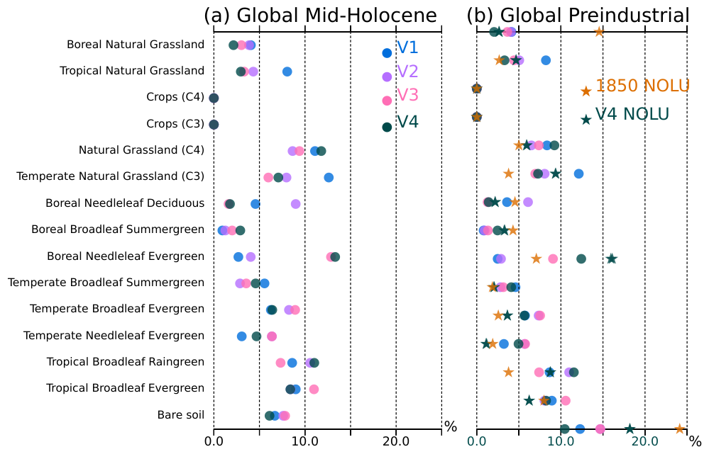
Figure 8 Percentage of global land surface covered by the different types of vegetation (PFT) for (a) the mid-Holocene and (b) the pre-industrial periods, as simulated by the four model versions (V1: blue, V2: green, V3: red and V4: black). The names of the different PFTs are plotted on the vertical axis. The stars in (b) represent the PFT distribution when ignoring grid points affected by land use in the pre-industrial (1850) vegetation map used as boundary condition when vegetation is prescribed (cyan for observations and black for V4).

All model versions, except V1, use barenew for bare soil evaporation. It appears to be a critical model aspect that contributes to a better representation of boreal forests. Bare soil evaporation is small in all simulations except V1 where it peaks in May–June (Fig. 9a), at a time when tree leaves are growing and soils are saturated in the Northern Hemisphere. With the bareold scheme, the evaporation is close to the potential evaporation under these conditions. The other simulations do not produce the large boreal spring bare soil evaporation. In these simulations, the evaporation is limited by soil and biomass characteristics (see Sect. 2.1). The evapotranspiration is slightly larger and peaks in July–August at the time of the maximum development of vegetation in the Northern Hemisphere (Fig. 9a). As a result, surface soil moisture is larger in V2 to V4 compared to V1, Fig. 9c), and favors tree growth.

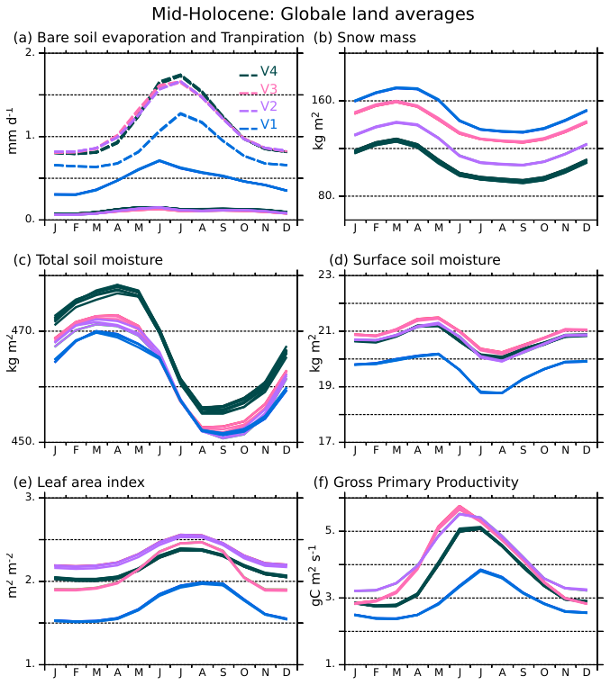
Figure 9 Annual cycle of mid-Holocene (a) bare soil evaporation (mm d⁻¹, solid lines) and transpiration (mm d⁻¹, dash lines), (b) snow mass (kg m⁻²), (c) total soil moisture (kg m⁻²), (d) surface soil moisture (kg m⁻²), (e) leaf area index (LAI) and (f) net assimilation of carbon by the vegetation (GPP, $\mathrm{g}\mathrm{C}{\mathrm{m}}^{-\mathrm{2}}{\mathrm{s}}^{-\mathrm{1}}$) globally averaged over land for the four simulations (V1: blue, V2: green, V3: red, and V4: black). All 100 year annual mean cycles, excluding the first 300 years, are plotted for each simulation in order to provide an idea of 100 years variability and show that the differences between the simulations are robust.

Large differences are also found in the distribution of the different grass PFTs across the mid-Holocene simulations. V1 has the largest proportion of Temperate (PFT 10) and Tropical (PFT 14) Natural Grasslands. It results from and contributes to the fact that V1 is the coldest simulation with the largest snow cover in regions covered by Temperate Grasslands (Fig. 9b). The partitioning between grass and tree leads to differences in root depths and in the way these different types of vegetation recycle water, which affects the soil moisture content (Fig. 9c). It affects temperature through evaporative cooling, which is further enhanced by snow in mid and high latitudes, and by reduced water vapor in the tropics. The large model spread found between the mid-Holocene simulations for 45–80° N albedos in the 0.3–0.7 range is the footprint of the difference in the ratio of tree and grass cover, with grass dominant vegetation for V1 and a mixture of grass and Boreal Needleleaf Deciduous (PFT 9) for V2 (Fig. 10). The peak emerging for albedo around 0.22 in V3 and V4 is related to their larger coverage of Boreal Needleleaf Evergreen (PFT 7) (Fig. 8). It highlights that the combination of tree and snow albedo leads to a smaller albedo in these two simulations. All the mid-Holocene simulations have a quite similar coverage of high albedo, which is compatible with the fact that they have a similar distribution of sea-ice and snow cover. The lower coverage for albedo>0.7 % is for V4, which has the smaller sea-ice cover and the largest proportion of low ocean albedo.

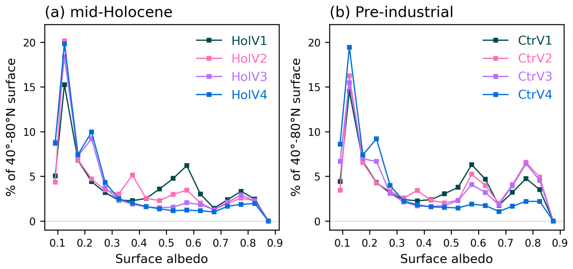
Figure 10 Distribution of the surface albedo (fraction of reflected radiation) as represented in the different simulations, considering all grid points between 45 and 80° N and months, for (a) the mid-Holocene and (b) the pre-industrial climates. For each albedo bin, the value represents the percentage of the surface with this particular albedo. The first bin (lower value) corresponds to ocean albedo. The higher values correspond to sea ice whereas values between 0.1 and 0.3 correspond to vegetation and bare soil, and values between 0.3 and 0.7 correspond to different mixtures of vegetation and snow albedo. The surface albedo has been computed using the surface upward and downward solar radiation.

In terms of radiative feedbacks between 45 and 80° N, the surface albedo effect varies significantly between the mid-Holocene simulations (Fig. 11a and b). The radiative feedbacks are computed using the Taylor et al. (2009) methodology, following what was done for the mid-Holocene differences with the pre-industrial climate in Sect. 3.2, In this case, 1 and 2 in Eq. (5) refer to model simulations performed with two different versions of the model. For this comparison, the V4 version of the model serves as reference. Positive values indicate that the feedback brings more energy to the climate system in V4. Since we compare the simulations for a given climate, the forcing is the same for all the mid-Holocene simulations, and the only factors affecting the global energy balance are the differences in seasonal climate feedbacks. The largest differences in surface albedo feedbacks between the V4 and the V1–V3 versions of the model occur from February to July. They are higher for V1 due to the largest snow-vegetation albedo feedback, as expected from the distribution of surface albedo between 45 and 80° N (Fig. 10). This effect exceeds 10 W m⁻² (up to about 16 W m⁻²) from April–June. The effect is smaller between V4 and V2 (up to 10 W m⁻²) or V4 and V3 (up to 8 W m⁻²). Note that for V2 and V3, the relative differences with V4 mainly originate from the relative distribution between the different types of boreal (PFT 7 or PFT 9) rather than from the different relative distribution between grass and forest (Fig. 10).

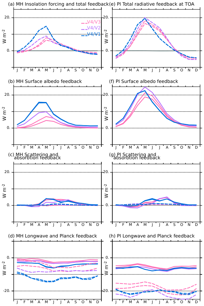
Figure 11 Estimation of radiative feedbacks (W m⁻²) induced by the differences in the land surface model and vegetation between the different model versions, using V4 as reference, for (a–d) the mid-Holocene simulations (MH) and (e–h) the pre-industrial simulations. Positive values indicate that more energy is entering the climate system at the top of the atmosphere in V4 than in the other version. As in Fig. 7, the different panels consider (a) and (e) the total radiative feedback, (b) and (f) the surface albedo feedback, (c) and (g) the atmospheric scattering (solid lines) and absorption (dashed lines), and (d) and (h) the outgoing longwave radiation feedback (solid lines) and the Planck response (dashed lines). The colours of the curves represent the different model versions.

The cloud SW feedback differences between the simulations slightly amplify the effect of the surface albedo from April to September in V1–V3 compared to V4 (Fig. 11c). Long wave radiation resulting from temperature, clouds and lapse rate partially balance the positive SW heat gain (Fig. 11d). This is mainly due to the differences in evapotranspiration between the mid-Holocene simulations (Fig. 9a) resulting from the combination of vegetation characteristics, but also from differences from the insulating effect of snow and ice cover in mid and high latitudes (Fig. 11). The Earth system model is equilibrated, which means that the global net heat flux at the top of the atmosphere is null. Therefore, the excess of energy between 45 and 80° N in V4 is compensated for by a radiative heat loss over all other regions. For example, the annual mean longwave feedback difference between V4 and V3 in the 45–80° N region is about $-\mathrm{1.5}\mathrm{W}{\mathrm{m}}^{-\mathrm{2}}$. It is not sufficient to balance the total positive shortwave radiative effect of about 3 W m⁻². This leads to an annual mean excess radiation flux of 1.5 W m⁻² entering the system in V4 compared to V3 in these latitudes. This excess of energy, integrated over the 45–80° N latitudes, is compensated by a negative equivalent annual mean budget difference averaged over all other regions. In these other regions, the warmer conditions in V4 lead to larger outgoing longwave radiation, which offsets the higher atmospheric greenhouse effect (not shown).

Figure 12 Zonal average differences in integrated atmospheric water content (kg m⁻²) between V4 and the other model versions for (a) the mid-Holocene climate (solid lines) and (b) the pre-industrial climate (dashed lines). The colours of the curves represent the model version: V1 (blue), V2 (green) and V3 (red). The different lines for a given model version have been computed considering all possible combinations of 100 year differences with V4. They provide an indication of the uncertainty.

Note that the largest differences in water content are found in the tropics and not in the 45–80° N region, with statistically significant differences found up to 40° S between V4 and the other model versions (Fig. 12). In the fully coupled system, rapid energy adjustment between the hemispheres and between land and ocean are induced by the regional differences in energy sinks and sources. These rapid teleconnections also shape the simulated climate mean state. Here, V4 is also warmer almost everywhere. The differences in atmospheric water content stress the important role of the tropics and tropical ocean in regulating the global atmospheric moisture and water vapour feedback.

4.2 Dependence of vegetation induced radiative feedbacks on mean climate state

The feedback differences between model versions discussed for the mid-Holocene and their seasonal evolution are similar to those occurring between the mid-Holocene and the pre-industrial climates for each model version (Sect. 3.3). However, the ranking in the strength of the feedback between the two comparisons (Figs. 6 and 11a–d) suggests that the strength of the feedback varies depending on the climate mean state, which is indeed the case (Fig. 11e–h).

The simulations all have in common consistent changes in vegetation between the mid-Holocene and pre-industrial climates (Figs. 7 and 8). At the global scale the larger fraction of bare soil and grasses simulated for the pre-industrial climate (Fig. 8) is consistent with the drying of the Sahara, and the southward retreat of the tree line in the Northern Hemisphere (Fig. 7). The magnitude of the difference between the two periods for each PFT is consistent with the distribution of each mid-Holocene PFT in each model version (Figs. 7 and 8). To first order, the distribution of vegetation appears thus as a factor characterizing a model version, as it does for present day to characterise regional climates.

However, notable differences are found that have implications for the quantification of the 45 and 80° N SW and LW seasonal radiative feedbacks (Fig. 11). For the pre-industrial period, the total radiative differences at the top of the atmosphere reache up to 20 W m⁻² in V4 compared to V2, and up to 25 W m⁻² in V4 compared to the other simulations. The differences found for V2 and V3 are as large as those found for V1 (Fig. 11e), which is not the case for the mid-Holocene (Fig. 11a). The larger pre-industrial sensitivity of these two simulations using PhotoCM5 is partly attributable to a larger impact of snow albedo (Fig. 10). For example, V3 and V4 have a similar fraction of Boreal Needleleaf Evergreen (PFT 7) in the mid-Holocene, but not in the pre-industrial climate (Fig. 8). Compared to the mid-Holocene climate, boreal forest is replaced by a larger fraction of Temperate Natural Grass (PFT 11) and bare soil (PFT 1) in V3. There is also a larger fraction of grass and bare soil in V2, whereas in V1, vegetation is dominated by grass and bare soil and doesn't change much (Fig. 8). There is thus a larger fraction of the points where the surface albedo is in the 0.5–0.7 range in V2 and V3 (Fig. 10). Significant differences between the pre-industrial simulations are also evident in the 0.7–0.9 snow and sea-ice albedo range (Fig. 10b). For V2 and V3, the number of points with low albedo value is also reduced, which reflects a larger increase in sea ice cover in these two simulations. The initial vegetation-albedo feedback is amplified by the sea-ice albedo feedback, which affects temperature, water vapor, and the crossing of different thresholds controlling vegetation growth.

The pre-industrial seasonal insolation forcing has a slightly different seasonal evolution and magnitude compared to the mid-Holocene. This is why the seasonal timing of the different feedbacks is slightly shifted in time (Fig. 11b and f). The magnitude of the atmospheric scattering effect between V4 and the other simulations is quite similar to what was obtained for the mid-Holocene (Fig. 11c and g). As for the mid-Holocene, V4 has a larger shortwave feedback leading to a positive excess of energy between 40 and 80° N compared to the other simulations. It implies that a negative feedback balances it over the other regions. This is achieved through the longwave feedback due to higher temperatures in V4. Interestingly, the difference in atmospheric water content is similar in the pre-industrial and mid-Holocene simulations between V4 and V1, whereas it is a factor of 2 in the pre-industrial compared to the mid-Holocene between V4 and V2 or V3. It is clearly tied to the amplitude of vegetation changes and sea-ice feedback, and thereby to the photosynthesis parameterization.

This comparison indicates that the relative magnitude of the vegetation-induced seasonal feedback between two climatic periods depends on the climate mean state. It also stresses that large differences in annual mean temperature in mid and high latitudes between the mid-Holocene and pre-industrial climates simulated with the different versions of the model (Fig. 3) come, for a large part, from the simulations of the pre-industrial climate, for which the largest differences are found between the V2 and V3 simulations using PhotoCM5 and the V4 simulation using PhotoCM6.

5 Discussion

5.1 Annual mean fingerprint of seasonal feedbacks

In the previous section, we showed that dynamic vegetation highlights how the seasonal evolution of vegetation triggers first-order atmospheric feedbacks. These large seasonal feedbacks have an annual mean fingerprint (Fig. 13).

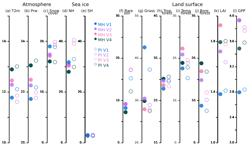
Figure 13 Mid-Holocene (MH, full circles) and pre-industrial (PI, circles) global annual mean for (a) Surface air temperature (T2m, °C), (b) Precipitable water content (kg m⁻²), (c) Snow cover over land (%), (d) Sea ice cover in the Northern Hemisphere, (e) Sea ice cover in the Southern Hemisphere (f) Bare soil (%), (g) Grass (%), (h) Tropical forest (%), (i) Temperate forest (%), (j) Boreal forest (%), (k) LAI, and (l) Gross primary production (GPP, ${\mathrm{10}}^{\mathrm{5}}\mathrm{g}\mathrm{C}{\mathrm{m}}^{-\mathrm{2}}{\mathrm{s}}^{-\mathrm{1}}$) and the four model versions (V1: blue, V2: green, V3: red and V4: black).

At the global scale, the warmest simulations are those run with the model version V4. The difference with the coldest simulation is about 1 °C. For each climatic period, the ranking between the simulations for the atmospheric water content is the same as the one for surface temperature. This is expected from the Clausius–Clapeyron relationship since the atmospheric and oceanic physics are the same between the model versions. An inverse ranking is found for snow and sea ice cover, resulting from the strong link between these variables and temperature (see Fig. 13d and e). However, the relative changes in snow and sea-ice cover between the model versions differ from those in temperature. The sea-ice feedback is an indirect effect. It is caused by temperature and atmospheric circulation changes that are driven by land surface feedbacks and their dependence on the mosaic vegetation. Model biophysical content and vegetation-climate temperature interactions lead to different vegetation cover. This results in different LAI and productivity (Fig. 13f–k). For each period, the warmest simulation is not necessarily the one with the largest LAI and productivity.

In Sect. 4, we also emphasised the climate state dependence of the seasonal feedbacks between the model versions. Vegetation cover is reduced in the pre-industrial climate compared to the mid-Holocene (Bigelow et al., 2003; Jolly et al., 1998; Prentice et al., 1996). However, depending on the choice of photosynthesis parameterisation, LAI and GPP are either reduced or slightly increased in the pre-industrial climate (Fig. 13k and l). Vegetation feedback results in a reduction in global mean temperature with photoCM5 and a larger increase in snow and sea-ice cover.

5.2 Role of the photosynthesis parameterization

The role of photosynthesis in regulating seasonal feedbacks needs to be highlighted. At the global scale, despite different distributions of vegetation, the two simulations with PhotoCM5 (V2 and V3) instead of PhotoCM6 (V1 and V4) exhibit a larger peak LAI during boreal summer (Fig. 9e), whatever the realism of the simulated vegetation. In V2 and V3, GPP has a strong increase from March–July when the peak GPP is reached (Fig. 9f). The LAI seasonality is smoother in V1 and V4. The parallel V1 and V4 LAI seasonal evolution reflects a similar behaviour with an offset resulting from differences in temperature and in vegetation coverage. The shape of PhotoCM5 as a function of temperature compared to PhotoCM6 (Fig. 1) favours larger productivity (GPP) as soon as LAI is developing. This means that for given climatic conditions, the start of the growing season should be similar with the two parameterisations, but photoCM5 should have larger gpp. This is indeed what we obtained between the simulations (Fig. 9e and f). This systematic difference affects the seasonality of the surface albedo, through the LAI and the total soil moisture. Reduced GPP during the growing season in the Northern Hemisphere implies less evapotranspiration leading to higher soil moisture, as it can be seen on Fig. 9 between V4 and V2 or V3, which are simulations sharing the same bare soil evaporation. Due to all the interactions in the climate system, we also end up with the counter intuitive result that V4 has the largest vegetation cover (Fig. 9), but that the vegetation is less productive than in V3 and even V2. Indeed, one would expect a larger LAI and GPP when vegetation cover is larger, which is a common reasoning when the way the photosynthesis is parameterised is not considered. Here we show that this simple reasoning is not valid, and that the shape of the photosynthesis function exerts a strong control on the linkage between changes in vegetation cover, LAI and GPP.

The major differences in the relationship between LAI and GPP discussed for the mid-Holocene (Fig. 9e and f) are also found for the pre-industrial climate (not shown). However, LAI is more similar between V3 and V4. The larger grass and bare soil fractions in V3 compensate for the tendency of this version of the model with PhotoCM5 to produce larger LAI. The critical threshold for tree mortality difference has a larger role for this period than for the mid-Holocene. Compared to the mid-Holocene climate, less insolation is received in mid and high latitudes during boreal summer. For both climates, the simulation using PhotoCM5 is colder. Therefore, the surface temperature is closer to the tcrit value in spring compared to the V4 simulation using PhotoCM6. It induces a larger reduction of the tree cover and of LAI and GPP (not shown) in V3 compared to V4. Indeed, with PhotoCM6, the pre-industrial seasonal vegetation growth follows the seasonal insolation forcing as for the mid-Holocene climate in V4. These seasonal behaviors and the nonlinear shape of photosynthesis as a function of temperature (Fig. 1) trigger the direction of the annual mean changes (Fig. 13).

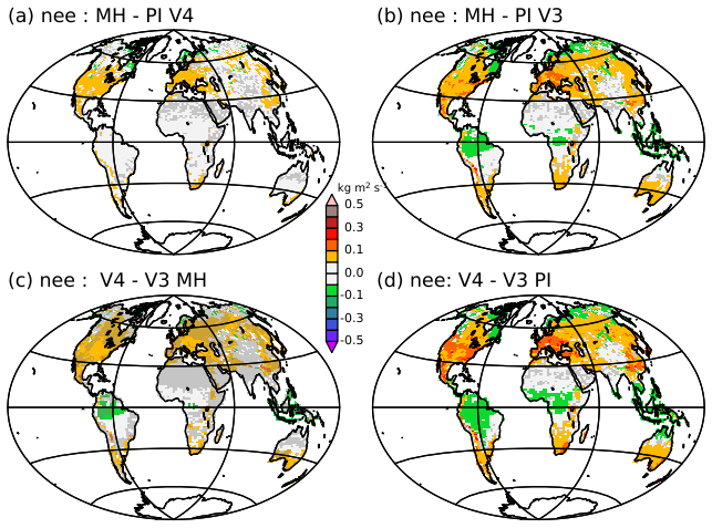
Figure 14 Net ecosystem exchange from the vegetation (kg m⁻² s) difference between (a) the mid-Holocene and the pre-industrial climates as simulated with version V4, (b) the mid-Holocene and the pre-industrial climate as simulated with version V3, (c) versions V4 and V3 for the mid-Holocene simulations, and (d) versions V4 and V3 for the pre-industrial simulations. A reduction of the carbon sink is indicated by a positive value, while an increase is indicated by a negative value. Changes are considered to be significant at the 5 % level outside the grey zones. The significance is estimated from all combinations of differences in 100 year averages between the simulations considered in each panel. For these estimates the first 300 years of the simulations are excluded.

The sensitivity of the photosynthesis parameterization to temperature has implications for the land-surface carbon feedbacks and the representation of the interactions between energy, water, and the carbon cycle in Earth system models. Here, the carbon dioxide concentration is prescribed in the atmosphere, but the carbon cycle is activated, so that carbon fluxes between the surface and the atmosphere can be diagnosed. Figure 14 illustrates that the annual mean pattern and magnitude of this flux are model version dependent. The carbon sink is reduced in V4 in mid-latitudes and increased in the tropics. It would lead to differences in regional and global carbon concentration in the atmosphere if carbon was fully interactive, and thereby certainly to different climate and vegetation characteristics.

5.3 Climate state dependence and model performance

We directly develop and tune the model using simulations of the mid-Holocene climate and not using simulations of the modern climate. Pre-industrial conditions were used to check if the model version was still valid for the conditions for which it was initially developed. The V3 and V4 versions of the model appear to be rather equivalent with respect to the simulated mid-Holocene vegetation and in broad agreement with the BIOME6000 reconstruction (Harrison, 2017). These versions benefit from all the adjustments but have different photosynthesis parameterisations. An in-depth model-data comparison would require transforming the 15 simulated PFTs into the equivalent biomes inferred from pollen (Prentice et al., 1996). It is out of the scope of this paper and would also introduce artificial choices (Braconnot et al., 2019; Dallmeyer et al., 2019). However, the simulated vegetation for the pre-industrial period is very different between these two model versions. The V3 simulation with PhotoCM5 produces the largest changes in vegetation and climate variables. These changes are larger than what is expected from temperature reconstructions by Bartlein et al. (2011), and mid to high latitudes are too cold with too much sea-ice in the pre-industrial period.

The simulations considered in this study were run considering only natural vegetation, even for the pre-industrial climate. Land use was estimated to lead to about 1–2 °C cooling in northern mid-latitude agricultural regions in winter and spring in comparison with their previously forested state (Betts et al., 2007). The quantification of the relative impact of climate and land use on Holocene vegetation by Marquer et al. (Marquer et al., 2017) also indicates that land use has become a dominant factor affecting natural vegetation changes and climate during the late Holocene. The results of our simulations thus cannot pretend to be realistic in regions affected by land use, such as Europe. An attempt to evaluate the simulated vegetation is provided in Fig. 8 by considering only grid points for which there is no land use in the pre-industrial climate. The stars on the figure correspond to the fraction occupied by each PFT for the V4 version and the reference 1850 vegetation map used when vegetation is prescribed to the model, as it is the case for CMIP6 pre-industrial simulations (Boucher et al., 2020). It suggests that, for the pre-industrial climate, the V4 version of the model overestimates the fraction of tropical forest (mainly PFT 3), has a reasonable representation of temperate forest (PFT 4–6), overestimates boreal forest (mainly PFT 7), and has a reasonable representation of grass, with the caveat that there is a misbalance between PFT 15 and PFT 11. Overall, it is quite reasonable and better than in the other versions (not shown). Since dand use, through its effect on temperature and evapotranspiration, has an indirect impact on the simulated natural vegetation both locally and remotely (Smith et al., 2016), a more in-depth model data comparison needs to be done using a simulation where both land use and dynamical vegetation are considered. Despite these limitations, the V4 model version provides the best compromise in the representation of the mid-Holocene and pre-industrial and has been retained for transient Holocene simulations with the IPSL model and dynamic vegetation.

The simulated vegetation is an integrator of all climate feedbacks. When considering climate variables, annual mean values are inappropriate if the seasonal cycle is a major contributor to climate change. Indeed, the global annual differences between the simulations reported in Fig. 13 are small, even though they are statistically significant, and result from differences in the simulated climate annual mean cycle. Our results stress the importance of targeting specific times of the year when key interactions and feedbacks occur for model-model or model-data comparisons. This is certainly also true for climate reconstructions. Depending on the method and records considered, substantial differences are found in annual mean reconstruction for the mid-Holocene climate (Brierley et al., 2020). The choice of records and physical or biogeochemical variable should thus be chosen depending on the feedback or process considered.

6 Conclusions

The suite of mid-Holocene and pre-industrial climate simulations considered here allows us to investigate how first-order albedo and water vapor feedbacks are triggered by land surface feedback induced by vegetation. We investigated the role of bare soil evaporation, photosynthesis, and temperature threshold determining boreal tree mortality. The results show that bare soil evaporation is a key factor controlling tree growth in mid and high latitudes. This effect doesn't affect the sign of the annual mean changes between mid-Holocene and pre-industrial climates. It has a major impact on the tree cover and affects temperature through the snow-vegetation-evaporation feedback loop. The major differences between the simulations come from the photosynthesis parameterization. The dynamic vegetation highlights the high impact this parameterisation has on the vegetation seasonal feedbacks and on the sign of the annual mean climate differences between the two periods. The way in which the photosynthesis parameterisation triggers vegetation growth and gross primary productivity regulates both the strength of the snow-vegetation feedbacks and how this feedback functions when temperature reaches the threshold temperature for tree mortality. This is independent of the exact representation of the vegetation cover, and similar processes would be found in other models with different atmospheric and oceanic physics. Indeed, despite the unavoidable radiative feedbacks induced vegetation induced changes in temperature and water vapour, the comparison between the different climates and model versions allows us to highlight the particular role of the photosynthesis parameterisation.

For a given climate period, the regional differences in feedbacks trigger changes in sources and sinks of energy. These feedbacks do not necessarily occur where changes occur on the land surface, but remotely, as it is the case for the water vapor in this study, which is maximum in the tropical regions when major snow-ice-vegetation albedo feedbacks are maximum in mid and high northern latitudes (Figs. 5 and 11). The remote LW radiative feedback is less discussed in the literature when the role of vegetation is inferred from vegetation-alone simulations or simulations where the sea surface temperature and sea-ice cover are prescribed. It is a first-order effect associated with the change in temperature (Dufresne and Bony, 2008; Manabe and Wetherald, 1975; Sherwood et al., 2020). It is often overlooked because it is the strongest over the tropical ocean, which is in general not part of the focus when analysing vegetation on land. A full understanding, and thereby the ability to improve Earth's system model simulations, requires studying vegetation feedbacks in the fully interactive ocean–atmosphere-vegetation coupled system.

The land surface feedbacks highlighted by the dynamical vegetation are present even when vegetation is prescribed, and our results indicate that they may not be satisfactorily represented. Dynamical vegetation should be considered in Earth System Model (i.e. climate models with an interactive carbon cycle) if one wishes to properly account for the way land surface would trigger cascading feedback effects depending on future climate pathways. This also means adding degrees of freedom in the system, and thereby potentially larger model biases or uncertainties, despite a more accurate representation of internal processes. Since a model cannot be perfect and targeted to answer all scientific questions, compromises need to be made between the realism of the simulated climate and the accuracy of the simulated processes, depending on the scientific question. The large sensitivity found for the growing season in the Northern Hemisphere suggests that this period in the year should be used to develop evaluation criteria that can be applied to offline land surface simulations on atmosphere–land interactions. This would help to anticipate the vegetation feedback behaviours when the land surface model is included in the coupled system.

Our results stress that further emphasis on seasonality is needed to better assess land-surface feedbacks and understand the sensitivity of the feedbacks to the climate mean state. They also emphasize that producing a model configuration that is suitable to address climate change questions both at the global and regional scale and across climate periods is still challenging, and that further understanding of the complex climate interactions and teleconnections requires adopting a coupled framework and reasoning. In addition, we show that the differences between the model versions in the simulation of the climate and vegetation differences between the mid-Holocene and the pre-industrial periods come mainly from the simulation of the pre-industrial climate. Direct model evaluation of the mid-Holocene climate, and not the differences with pre-industrial conditions, would be required to fully infer the realism of the simulated climate. Paleoclimate periods for which the major differences with present day come from the annual cycle of the insolation forcing, such as the mid-Holocene discussed here or the last interglacial periods considered as part of PMIP (Kageyama et al., 2018; Otto-Bliesner et al., 2017), are well-suited to provide observational constraints on these feedbacks. They provide direct and indirect indications of the seasonal evolution on temperature, precipitation, sea-ice cover, or vegetation. This is a direction to consider for future research that would help better infer the ability of a model to simulate the annual mean cycle.