100 kyr ice age cycles as a timescale-matching problem

The dominant period of the Late Pleistocene glacial–interglacial cycles is roughly 100 kyr, rather than other major astronomical periods such as 19, 23, 41, and 400 kyr. Various models explain this fact through distinct dynamical mechanisms, including synchronization of self-sustained oscillations and resonance in mono- or multi-stable systems. However, the diversity of proposed models and dynamical mechanisms may obscure the essential factor behind the emergence of the ∼100 kyr periodicity. We propose the hypothesis that the ice-sheet climate system responds to astronomical forcing at the ∼100 kyr periodicity because the intrinsic timescale of the system is closer to 100 kyr than to other major astronomical periods. We support this idea with analyses and sensitivity studies of several simple ice age models with contrasting mechanisms.

1 Introduction

Glacial–interglacial cycles are a pronounced mode of climate variability in the Pleistocene, accompanied by large changes in temperatures (Clark et al., 2024; Jouzel et al., 2007), global ice volume (Rohling et al., 2022), and greenhouse gas concentrations (Bereiter et al., 2015; Lüthi et al., 2008). Changes in global ice volume are recorded, e.g., in the oxygen isotope ratio δ¹⁸O of benthic foraminifera found in marine sediments (Lisiecki and Raymo, 2005) (Fig. 1d), where higher δ¹⁸O values indicate larger ice volume and lower deep-ocean temperatures. The dominant period of the Late Pleistocene glacial cycles is roughly 100 kyr, as shown in the power spectral density (PSD) (Fig. 1f; see Appendix A for the PSD method).

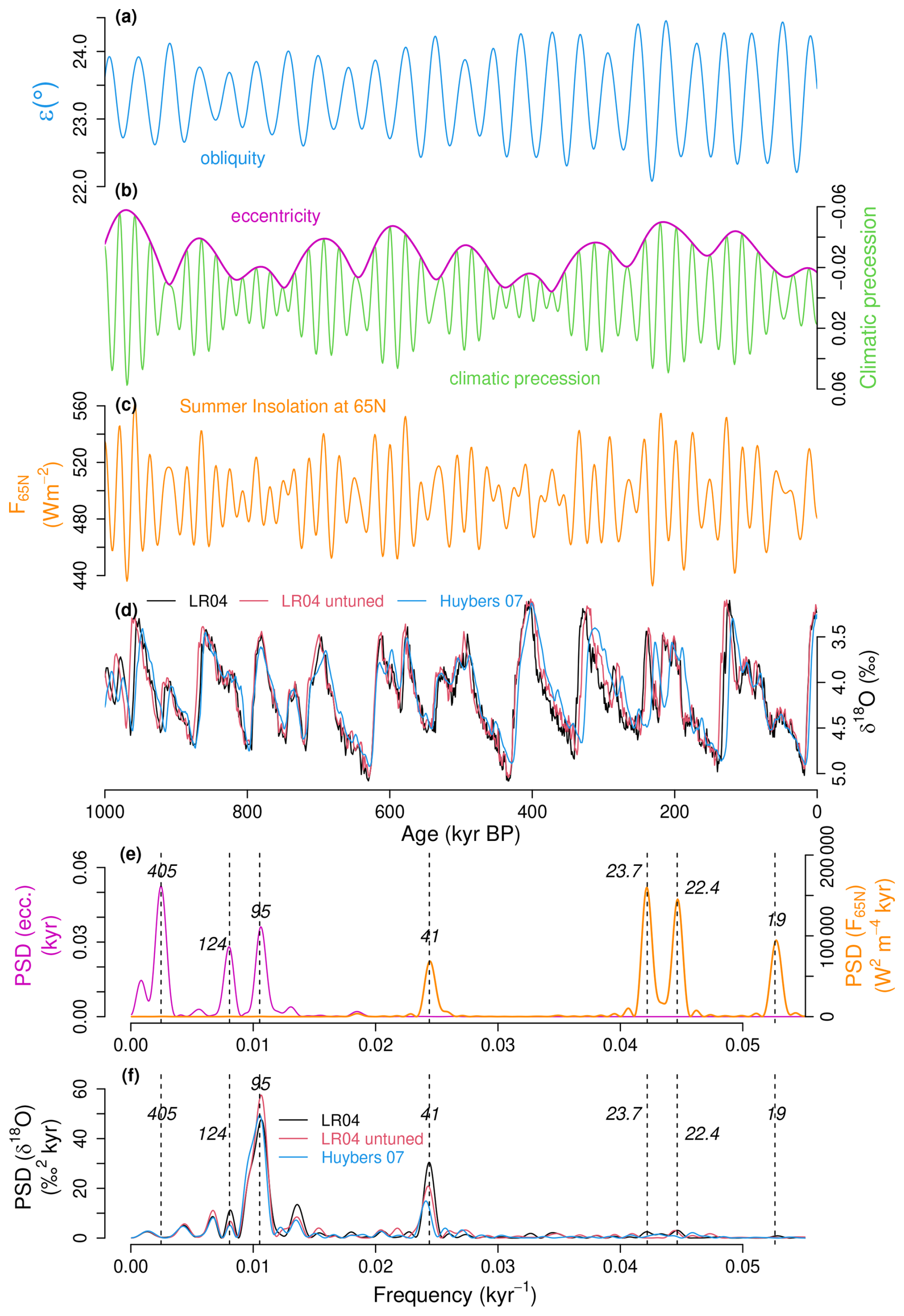
Figure 1 Time series and power spectral densities (PSDs) of the astronomical forcing (Laskar et al., 2004) and glacial cycles over the last 1 Myr. (a) Obliquity. (b) Climatic precession (green) and eccentricity (magenta). (c) Summer solstice insolation at 65° N. (d) Benthic δ¹⁸O stack records representing glacial–interglacial cycles. The so-called LR04 record with orbital tuning (black) (Lisiecki and Raymo, 2005), the LR04 record without orbital tuning (red) (Lisiecki, 2010), and the record without orbital tuning (blue) (Huybers, 2007). Note that the vertical axis is reversed so that larger δ¹⁸O values, corresponding to colder conditions, are lower. (e) PSD of the eccentricity (magenta) and the PSD of the summer solstice insolation F_65N (orange). (f) PSDs from each benthic δ¹⁸O record in (d). The dashed vertical lines in (e) and (f) indicate major astronomical periods (Laskar et al., 2004).

Summer insolation in the high northern latitudes (Fig. 1c) is supposed to be a major driver (Milankovitch, 1941; Roe, 2006) or a pacemaker (Hays et al., 1976) of the glacial–interglacial cycles. It fluctuates due to long-term variations in the astronomical parameters: climatic precession esin ϖ (and co-precession ecos ϖ) with 19, 22.4, and 23.7 kyr dominant periods (Fig. 1b, green); obliquity ε with a 41 kyr period (Fig. 1a); and eccentricity e with 95, 124, and 405 kyr periods (Fig. 1b, magenta) (Laskar et al., 2004; Berger, 1978), where the periods of eccentricity are linked with those of climatic precession by relations of combination tones such as $\mathrm{1}/\mathrm{95}\simeq \mathrm{1}/\mathrm{19}-\mathrm{1}/\mathrm{23.7}$ (Berger et al., 2005). These astronomical periods are in fact imprinted in the PSDs of the δ¹⁸O records, as shown in Fig. 1f (Hays et al., 1976).

However, despite the dominant average period of the Late Pleistocene glacial cycles being ∼100 kyr, the boreal summer insolation only has negligible power at this frequency. This discrepancy is known as the 100 kyr problem. Instead, boreal summer insolation exhibits strong power in the 19–23.7 kyr precession band and the 41 kyr obliquity band (Fig. 1e, orange). Hence, the ∼100 kyr glacial cycles have previously been explained as a response to four or five precession cycles (Ridgwell et al., 1999; Cheng et al., 2009; Hobart et al., 2023), a response to two or three obliquity cycles (Huybers and Wunsch, 2005), or a combination thereof (Huybers, 2011; Tzedakis et al., 2017; Ryd and Kantz, 2024). Note that a single response to four or five precession cycles generally coincides with a one-to-one response to ∼100 kyr eccentricity cycles, since a deglaciation in response to climatic precession esin ϖ tends to occur near the rising limb of eccentricity e (Raymo, 1997; Abe-Ouchi et al., 2013). Thus, eccentricity seems to impact the pace of glacial cycles via the modulation of climatic precession, even though the boreal summer insolation forcing only has negligible 100 kyr power.

Until now, we have referred to the dominant period of the Late Pleistocene glacial cycles as ∼100 kyr. Examining the PSDs of the benthic δ¹⁸O stack records over the last 1 Myr (Lisiecki and Raymo, 2005), the ∼100 kyr spectral peak actually aligns with the 95 kyr eccentricity peak, and it is indeed distinct from other potential eccentricity peaks such as 124 kyr (Fig. 1e and f). Concerns could be raised about using a tuned record for such an assessment, but the same conclusion is also drawn from two other records that are free from orbital tuning (Lisiecki, 2010; Huybers, 2007). Thus, in this study, the 95 kyr period is assumed as the strongest mode over the last 1 Myr (Clark et al., 2024, and Rial, 1999, also specifically state the 95 kyr period). This strong imprint of the 95 kyr eccentricity period (i.e., the combination tone of the climatic precession periods 23.7 and 19 kyr) is consistent with recent studies suggesting that the timings of deglaciations are more tightly coupled with multiple climatic precession cycles than multiple obliquity cycles with 82 or 123 kyr (Hobart et al., 2023; Cheng et al., 2016; Abe-Ouchi et al., 2013).

Synchronization and nonlinear resonance are two major dynamical mechanisms that result in a system's response tightly coupled with external forcing. Due to their ubiquity in nature, they are often invoked to explain the emergence of ∼100 kyr cycles. As they are central to the discussion that follows, we briefly review them below.

In synchronization (a.k.a. frequency entrainment, phase locking, or frequency locking)¹, the system is assumed to exhibit self-sustained oscillations in the absence of forcing, and the frequency of the underlying oscillations is adjusted to match one of the frequencies of external forcing, its harmonics, subharmonics, or a combination of these (Pikovsky et al., 2003). Many ice age models generate ∼100 kyr cycles through the synchronization mechanism (Saltzman et al., 1984; Gildor and Tziperman, 2000; Ashkenazy and Tziperman, 2004; De Saedeleer et al., 2013; Crucifix, 2013; Ashwin and Ditlevsen, 2015; Nyman and Ditlevsen, 2019; Mitsui et al., 2015, 2023; Koepnick and Tziperman, 2024). Synchronization occurs more easily when the frequency of external forcing is closer to the natural frequency of the system's underlying self-sustained oscillations (Pikovsky et al., 2003). Thus if the ∼100 kyr cycles are realized via synchronization, it suggests the existence of underlying self-sustained oscillations at ∼100 kyr timescale.

Resonance, on the other hand, refers to an enhanced output response to an external forcing. Linear resonance is well known, in which the response to a periodic forcing is amplified when the external frequency Ω matches the system's natural frequency ω₀. In nonlinear systems, more complex behavior called nonlinear resonances occurs, such as the following: (i) the resonant frequency Ω_r that yields the maximum response can deviate from the natural frequency ω₀ as the forcing amplitude increases; (ii) resonances can occur at superharmonics mΩ, subharmonics $\mathrm{\Omega }/n$, and supersubharmonics $m\mathrm{\Omega }/n$, where $m,n\in \mathbb{N}$ (Jackson, 1989). Recently, the term resonance has been generalized to include a broader range of processes that involve the enhancement, suppression, or optimization of a system's response through the variation, perturbation, or modulation of any system property (Rajasekar and Sanjuan, 2016). In nonlinear resonance mechanisms of ∼100 kyr ice age cycles, the underlying system is commonly assumed to be mono- or multi-stable, and the system's response to 19–23.7 and 41 kyr forcings is nonlinearly amplified at ∼100 kyr timescale (Ryd and Kantz, 2024), for example, at the combination tone $\mathrm{1}/\mathrm{95}=\mathrm{1}/\mathrm{19}-\mathrm{1}/\mathrm{23.7}$ kyr⁻¹ (Le Treut and Ghil, 1983). Many studies, however, use the terms nonlinear response (Ganopolski, 2024; Ashkenazy and Tziperman, 2004) or nonlinear amplification (Verbitsky et al., 2018) to refer to cases compatible with the generalized notion of resonance. Other types of resonance have been discussed in relation to the ∼100 kyr cycles, including linear resonance (Hagelberg et al., 1991; Ditlevsen et al., 2020), stochastic resonance (Benzi et al., 1982; Nicolis, 1981), coherence resonance (Pelletier, 2003; Bosio et al., 2023), and vibrational resonance (Ryd and Kantz, 2024).

Despite such differences in dynamical mechanisms and underlying system types, several ice age models with distinct approaches successfully simulate proxy records with similar accuracy, reproducing the ∼100 kyr cycles. This raises an important question: if models with different mechanisms can reproduce the glacial cycles, what is the key factor that enables the ∼100 kyr cycles, regardless of the specific mechanism? To address this question, we examine three previously proposed ice age models, each representing a different mechanism and underlying system type: one based on synchronization, one on resonance in a mono-stable system, and one on resonance in a multi-stable system with thresholds. Through sensitivity experiments changing the model's internal timescale and the amplitude of the forcing, we reveal that the key to enabling the 100 kyr cycles is the proximity of the intrinsic timescale of the underlying climate system to the ∼100 kyr periodicity of eccentricity cycles. Our results suggest that periodicity around ∼100 kyr occurs because of the match between the Earth system's intrinsic timescale and one astronomic timescale.

The remainder of this article is organized as follows. In Sect. 2 we present the three simple models of ice age cycles with different mechanisms for generating ∼100 kyr cycles. In Sect. 3, we conduct sensitivity experiments by artificially varying the system's intrinsic timescale, demonstrating that it plays a crucial role in producing ∼100 kyr cycles, regardless of the underlying mechanism. Section 4 is devoted to the discussion. In Sect. 5, we conclude the article.

2 Models for glacial cycles

2.1 Self-sustained oscillator (SO) model representing the synchronization mechanism

A paradigmatic dynamical system featuring self-sustained oscillations is the oscillator of Van der Pol (1926). Crucifix and colleagues have used the forced van der Pol oscillator as a mathematical model to investigate ice age dynamics (Crucifix, 2012, 2013; De Saedeleer et al., 2013). We consider a generalized version of the model:

$$\begin{array}{}\text{(1)}& {\displaystyle }& {\displaystyle }\dot{x}=y+\mathit{\kappa }x-{\displaystyle \frac{\mathit{\mu }}{\mathrm{3}}}{x}^{\mathrm{3}}\text{(2)}& {\displaystyle }& {\displaystyle }\dot{y}=-\mathit{\alpha }x-\mathit{\beta }{x}^{\mathrm{3}}-\mathit{\theta }-(\mathit{\nu }+\mathit{\rho }x)I\left(t\right)-\mathit{\eta }{I}^{\mathrm{2}}\left(t\right),\end{array}$$

with $y={\mathit{\delta }}^{\mathrm{18}}\mathrm{O}-\mathit{\delta }-\mathrm{4}$, linking the variable y with the ice volume proxy δ¹⁸O with an offset δ+4. Variable x abstractly represents the “climate” state that determines whether the system is in the glaciation or the deglaciation phase, in combination with the insolation. It could represent the oceanic state (De Saedeleer et al., 2013), the carbon cycle, dust concentrations, or their mixed effect. Variable I(t) is the standardized summer solstice insolation anomaly at 65° N, and the model's parameters are denoted with Greek labels. The nonlinear term ηI²(t) is included to take into account the lower sensitivity of the ice volume in the cold period (Paillard, 1998). Equations (1) and (2) contain not only the van der Pol equation but also the equation of Duffing (1918) due to the cubic term βx³, and the Hill equation (Magnus and Winkler, 2004) due to the multiplicative force ρxI(t) (see Appendix B for details). Thus, it is expected to have greater flexibility to accommodate complex nonlinear oscillations than the original forced van der Pol equation.

The parameters in Eqs. (1) and (2) and δ are tuned to minimize the mean squared errors between the simulated and observed δ¹⁸O records over the last 1 Myr (see Appendix B). The model reproduces the record of glacial cycles quite well (Fig. 2b, pink; R=0.88) including the 95 kyr periodicity (Fig. S2c in the Supplement). For zero insolation anomaly I(t)=0, the underlying system possesses self-sustained oscillations with a period of 91.7 kyr (Fig. 2b, sky blue). Such self-sustained oscillations occur over a range of insolation anomaly $-\mathrm{0.66}<I<\mathrm{0.075}$. The oscillation period varies moderately over the range $-\mathrm{0.66}<I<\mathrm{0.075}$ with a mean of about 90 kyr (Fig. S1 in the Supplement). The internal oscillations capture the slow buildup and the rapid disintegration of ice sheets. Under the astronomical forcing, the frequency entrainment occurs mainly at $\mathrm{1}/\mathrm{95}$ kyr⁻¹ near that of self-sustained oscillations, $\mathrm{1}/\mathrm{91.7}$ kyr⁻¹. Equations (1) and (2) are hereafter called the Self-sustained Oscillator (SO) model.

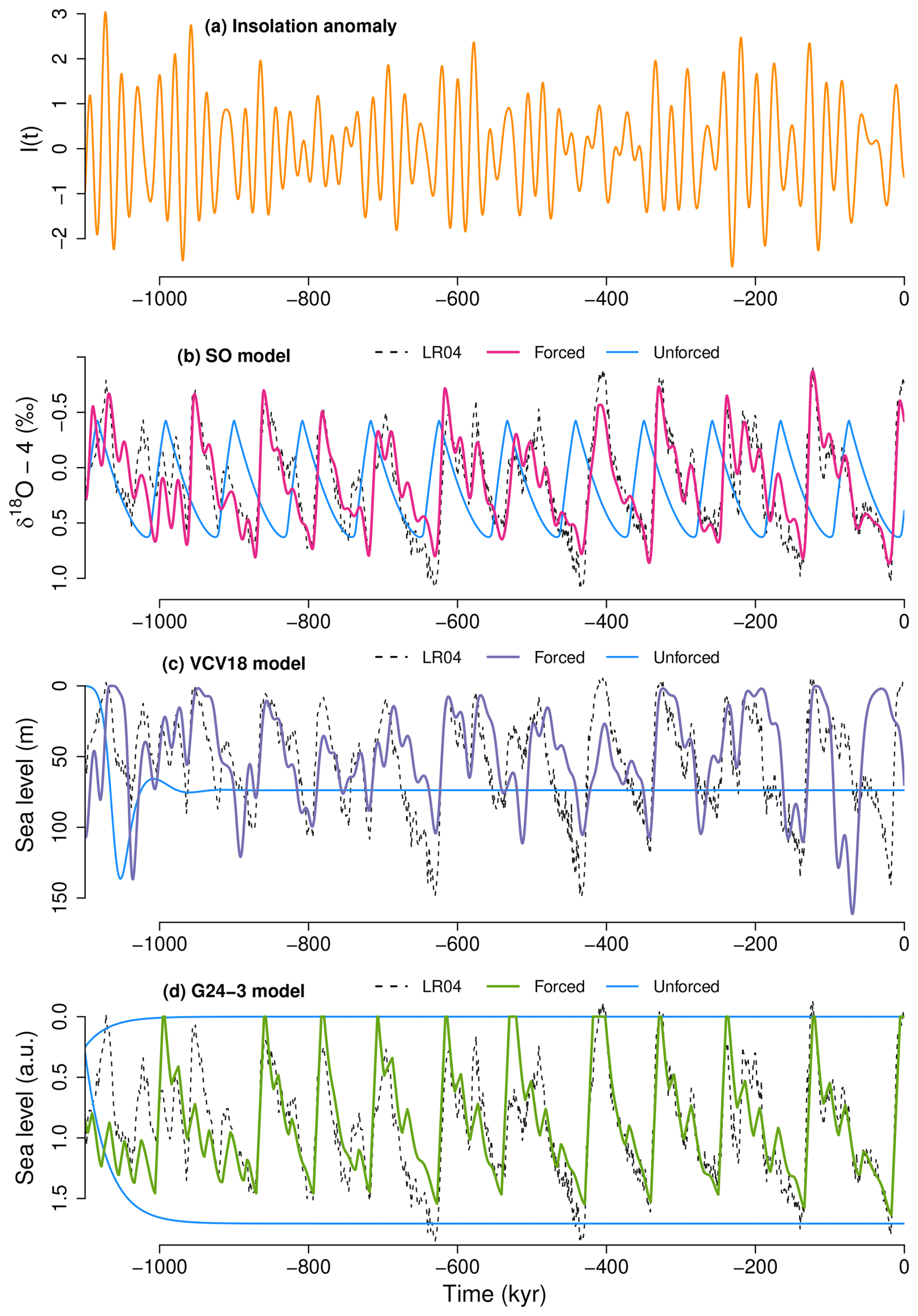
Figure 2 Forced and unforced simulations of glacial cycles over the last 1 Myr: (a) standardized summer solstice insolation at 65° N. (b) SO model with forcing (pink) and without forcing (light blue). (c) VCV18 model with forcing (violet) and without forcing (light blue). (d) G24-3 model with forcing (green) and without forcing (light blue). For all three models, the corresponding scaled versions of the paleoclimatic record are shown by the black dashed line.

2.2 Verbitsky–Crucifix–Volobuev model representing the resonance mechanism in monostable system

Verbitsky et al. (2018) introduced a simple model of ice age cycles deduced from a scaling analysis of the governing physical laws (hereafter VCV18 model). The equations for the glaciation area (S), the basal temperature (θ), and the ocean temperature (ω) are given by

$$\begin{array}{ll}{\displaystyle }& {\displaystyle }\dot{S}={\displaystyle \frac{\mathrm{4}}{\mathrm{5}}}{\mathit{\zeta }}^{-\mathrm{1}}{S}^{\mathrm{3}/\mathrm{4}}(a-\mathit{\epsilon }I(t)-\mathit{\kappa }\mathit{\omega }-c\mathit{\theta })\\ {\displaystyle }& {\displaystyle }\dot{\mathit{\theta }}={\mathit{\zeta }}^{-\mathrm{1}}{S}^{-\mathrm{1}/\mathrm{4}}(a-\mathit{\epsilon }I(t)-\mathit{\kappa }\mathit{\omega })\mathit{\{}\mathit{\alpha }\mathit{\omega }+\mathit{\beta }[S-S_{\mathrm{0}}]-\mathit{\theta }\mathit{\}}\\ {\displaystyle }& {\displaystyle }\dot{\mathit{\omega }}={\mathit{\gamma }}_{\mathrm{1}}-{\mathit{\gamma }}_{\mathrm{2}}[S-S_{\mathrm{0}}]-{\mathit{\gamma }}_{\mathrm{3}}\mathit{\omega },\end{array}$$

where I(t) is the standardized summer solstice insolation at 65° N. The ice volume is given as $V=\mathit{\zeta }{S}^{\mathrm{5}/\mathrm{4}}$. See Table 1 in Verbitsky et al. (2018) for the parameter values. Since the system becomes numerically unstable near S=0, we reset the S value to 10⁻⁴ if it falls below 10⁻⁴. The VCV18 model can roughly simulate changes in sea level as shown in Fig. 2c (violet). Although the simulated sea level does not capture the amplitude and timing of all deglaciations (specifically, the last one), the model exhibits prominent ∼100 kyr power consistently with the record (Fig. S3c in the Supplement). In the absence of forcing (I(t)≡0), the system has a single stable equilibrium whose Jacobian matrix has one real negative eigenvalue and a pair of complex conjugate eigenvalues with negative real parts. The imaginary part of the latter pair defines the natural frequency of the system. In this article, we refer to the inverse of the natural frequency as the natural period. Under the standard parameter set, this natural period is 95 kyr.

Although the astronomical forcing has most of its power at ∼20 and 41 kyr bands, the dominant power in the climate response is concentrated near ∼100 kyr. Since the system does not exhibit self-sustained oscillations, the appearance of ∼100 kyr cycles in the VCV18 model cannot be qualified as a phenomenon of synchronization. Instead, it must be related to a nonlinear amplification of the response (Verbitsky et al., 2018), i.e., nonlinear resonance, as shown in Sect. 3.

2.3 Ganopolski model representing the resonance mechanism in multistable systems

Ganopolski (2024) discusses three simple models of ice age cycles in his Generalized Milankovitch Theory (hereafter G24-1,2,3). The G24-3 model is a model derived from ice age simulations using the Earth system model of intermediate complexity CLIMBER-2 (Calov and Ganopolski, 2005; Ganopolski and Calov, 2011; Willeit et al., 2019). The change in ice volume v is defined in the glaciation and deglaciation regimes, respectively, as

$${\displaystyle }{\displaystyle }\dot{v}=\left\{\begin{array}{ll}\frac{V_{\mathrm{e}}-v}{t_{\mathrm{1}}}& \text{if }k=\mathrm{1}\text{ (glaciation regime)}\\ -\frac{v_{\mathrm{c}}}{t_{\mathrm{2}}}& \text{if }k=\mathrm{2}\text{ (deglaciation regime)},\end{array}\right.$$

where t₁=30 and t₂=10 kyr are relaxation timescales in each regime estimated from CLIMBER-2 experiments (Calov and Ganopolski, 2005). The term V_e represents either of two stable equilibria depending on the state v and the 65° N summer solstice insolation anomaly f(t) relative its mean over the last 1 Myr:

$${\displaystyle }{\displaystyle }{V}_{\mathrm{e}}\left(f\right)=\left\{\begin{array}{ll}{V}_{\mathrm{g}}\left(f\right)& \text{if }f<f_{\mathrm{1}}\text{, or }{f}_{\mathrm{1}}<f<f_{\mathrm{2}}\text{ and }v>V_{\mathrm{u}}\left(f\right)\\ V_{\mathrm{i}}& \text{if }f>f_{\mathrm{2}}\text{, or }{f}_{\mathrm{1}}<f<f_{\mathrm{2}}\text{ and }v<V_{\mathrm{u}}\left(f\right),\end{array}\right.$$

where $f_{\mathrm{1}}\le f\le f_{\mathrm{2}}$ is the range of multiple equilibria, with $f_{\mathrm{1}}=-\mathrm{16}$ and f₂=16 Wm⁻². The function $V_{\mathrm{g}}\left(f\right)=\mathrm{1}+\sqrt{\frac{f_{\mathrm{2}}-f}{f_{\mathrm{2}}-f_{\mathrm{1}}}}$ represents the glacial equilibrium, and V_i=0 is the interglacial equilibrium. The unstable equilibrium separating the glacial and interglacial basins is given by $V_{\mathrm{u}}\left(f\right)=\mathrm{1}-\sqrt{\frac{f_{\mathrm{2}}-f}{f_{\mathrm{2}}-f_{\mathrm{1}}}}$ (see Fig. 4 in Ganopolski, 2024). Note that f(t) is an anomaly and not scaled by its standard deviation, different to I(t) in the previous two models. The transition from the glaciation regime (k=1) to the deglaciation regime (k=2) occurs if three conditions are met: v>v_c, f>0, and $\dot{f}>\mathrm{0}$, where v_c(=1.4) is the critical ice volume, above which the ice sheets are likely to collapse. The transition from the deglaciation regime (k=2) to the glaciation regime (k=1) occurs if f drops below f₁. Since v should remain non-negative, we reset it to 0 at each integration time step if it becomes negative.

The G24-3 model simulates the glacial cycles well (R=0.82 over 1 Myr) and has two stable equilibria for f=0 (Fig. 2d). By construction, the G24-3 model does not produce self-sustained oscillations for constant insolation because its regime transitions require threshold crossings in insolation. Ganopolski (2024) mentions that the characteristic timescales of the model are t₁=30 and t₂=10 kyr, and the model has no intrinsic timescale close to 100 kyr. However, the intrinsic timescale of the G24-3 model may be considered much longer than the relaxation times t₁=30 and t₂=10 kyr. First, assuming the average insolation f=0, the time in which the ice volume increases from v=0 to the critical ice volume v_c is $t_{\mathrm{1}}\ln \frac{V_{\mathrm{g}}\left(\mathrm{0}\right)}{V_{\mathrm{g}}\left(\mathrm{0}\right)-v_{\mathrm{c}}}\approx \mathrm{51.5}$ kyr. Even after the ice volume exceeds v_c, the ice sheets continue to grow until the insolation anomaly f changes from negative to positive. While this time lag varies depending on the phase of the precession cycles, half of the precession period, approximately 10 kyr, is a reasonable expected value. Adding this lag on top of 51.5 kyr, the total period from glacial inception to the onset of deglaciation is estimated as 61.5 kyr. Second, the time it takes for the ice to melt is about t₂=10 kyr. After this period of deglaciation, which usually continues during f>0, the system waits for glacial inception triggered by the drop in f below f₁. This waiting time is roughly $\mathrm{1}/\mathrm{4}$ precession cycle, i.e., ∼5 kyr. The sum of the glaciation timescale and the deglaciation timescale for G24-3 model is $t_{\mathrm{1}}\ln \frac{V_{\mathrm{g}}\left(\mathrm{0}\right)}{V_{\mathrm{g}}\left(\mathrm{0}\right)-\mathrm{1.5}}+t_{\mathrm{2}}=\mathrm{61.5}$ kyr, while the timescale to complete a cycle including the time lags is $t_{\mathrm{1}}\ln \frac{V_{\mathrm{g}}\left(\mathrm{0}\right)}{V_{\mathrm{g}}\left(\mathrm{0}\right)-\mathrm{1.5}}+t_{\mathrm{2}}+\mathrm{15}=\mathrm{76.5}$ kyr. This timescale is closer to the 95 kyr eccentricity period than other fundamental astronomical periods.

3 Sensitivity experiments

In the previous section, we showed that the three models of ice age cycles exhibit distinct types of underlying dynamics, each having a characteristic timescale: the period of a self-sustained oscillation, the period corresponding to the natural frequency (i.e., natural period), and the timescale for forming a cycle. These system's intrinsic timescales are schematically illustrated in Fig. 3. Here, we conduct sensitivity experiments on the models described in Sect. 2 to demonstrate that an intrinsic timescale close to ∼100 kyr is the key to enabling a periodicity around 100 kyr in all three types of models.

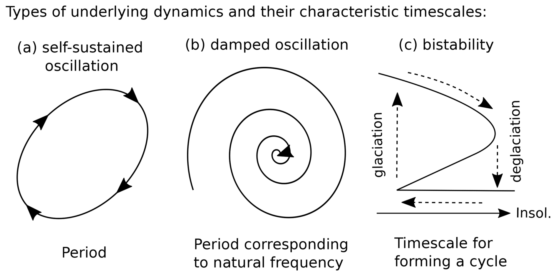
Figure 3 Three types of proposed underlying dynamics of ice age cycles and their characteristic timescales. (a) Self-sustained oscillation with a period. (b) Damped oscillation characterized by a period corresponding to the natural frequency. (c) A bistable system characterized by a timescale for forming a cycle, which includes the timescale of glaciation, the timescale of deglaciation, the time lag before glaciation is triggered by insolation, and the time lag before deglaciation is triggered.

3.1 Responses to the astronomical forcing

First, we show that the three models exhibit different responses to astronomical forcing. The models are run with a scaled insolation forcing: $\stackrel{\mathrm{̃}}{I}\left(t\right)=AI\left(t\right)$ in the SO model and the VCV18 model and $\stackrel{\mathrm{̃}}{f}\left(t\right)=Af\left(t\right)$ in the G24-3 model. The original simulations correspond to A=1. The changes in the PSD for varying A in steps of 0.02 are shown in Fig. 4. Specific time series and PSDs for A=0, 0.5, 1, 1.5, and 2 are shown in Figs. S2–S4 in the Supplement.

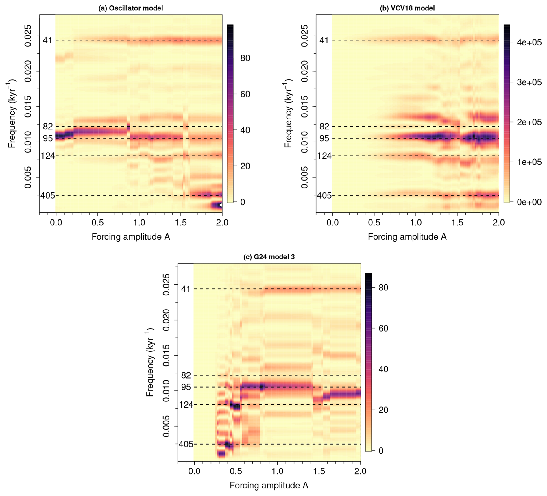
Figure 4 Power spectral density (PSD) for different amplitudes A of the astronomical forcing: (a) SO model. (b) VCV18 model. (c) G24-3 model. The PSDs are obtained from simulations over the last 1 Myr. The magenta dashed lines indicate the major astronomical frequencies (the numbers show the corresponding periods). The precession band, 19–23 kyr, is not shown since its power is comparatively minor.

In the SO model, as shown in Fig. 4a, the PSD has its maximum at 91.7 kyr for zero forcing amplitude, A=0, corresponding to self-sustained oscillations. For small A≤0.84, frequency locking to a major astronomical period is not achieved (Fig. S2a and b in the Supplement). The frequency locking to a 82 kyr double-obliquity period is realized for a very narrow range $\mathrm{0.86}\le A\le \mathrm{0.88}$. The frequency locking at 95 kyr occurs for a wide range of $\mathrm{0.90}\le A\le \mathrm{1.52}$. For larger A, the principal period shifts toward the larger side, exhibiting frequency lockings to 124 or 405 kyr.

In the VCV18 model shown in Fig. 4b, the total power is quite small for low A since the underlying dynamics is a damped oscillation. For A less than half of the original value, the PSD has a maximum at 41 kyr, although it is too small to be clearly seen in Fig. 4b. This is simply the linear response to the 41 kyr obliquity cycles. A large power appears at the 95 kyr eccentricity period as A increases to more than 0.5. This resonance with 95 kyr eccentricity cycles is actually a nonlinear resonance to the combination tone between 19–23.7 kyr precession cycles. This nonlinear resonance is found near the system's natural period of 95 kyr. This is in line with the classical notion that the resonance typically occurs if the frequency of external forcing matches the natural frequency of the system.

In the G24-3 model shown in Fig. 4c, the power is zero for low forcing amplitude A≤0.36 because glacial inception cannot be triggered. Glacial inception is possible for A≥0.38. The main peak is located at 405 kyr for $\mathrm{0.38}\le A\le \mathrm{0.42}$, at 124 kyr for $\mathrm{0.44}\le A\le \mathrm{0.54}$, and at 95 kyr for the wide range of $\mathrm{0.56}\le A\le \mathrm{1.42}$. This occurs because the frequency of threshold crossing increases as A increases. The principal period remains close to 100 kyr for larger A(≥1.44), but it is different from any major astronomical period.

3.2 Intrinsic timescales and responses

Next, we investigate the relationship between the principal period of the output and the intrinsic timescale of the model. For this purpose, we introduce a parameter r that modulates the timescale of the model, following previous studies (De Saedeleer et al., 2013; Crucifix, 2013). Each dynamical equation is scaled as $r\frac{\mathrm{d}X}{\mathrm{d}t}=\text{r.h.s}$. The larger r, the slower the temporal variation of the model variables. In the SO model, the period of self-sustained oscillations (originally T₀=91.7 kyr) is scaled as rT₀. Similarly, in the VCV18 model, the natural period of the damped oscillations (originally T₀=95 kyr) becomes rT₀. In the G24-3 model, the intrinsic timescale for the glaciation and deglaciation is scaled as $r\left(t_{\mathrm{1}}\ln \frac{V_{\mathrm{g}}\left(\mathrm{0}\right)}{V_{\mathrm{g}}\left(\mathrm{0}\right)-v_{\mathrm{c}}}+t_{\mathrm{2}}\right)=\mathrm{61.5}r$ kyr. Adding the time lags required for the astronomical conditions to be met, the timescale for forming a cycle is $T_{\text{cyc}}\left(r\right)=r\left(t_{\mathrm{1}}\ln \frac{V_{\mathrm{g}}\left(\mathrm{0}\right)}{V_{\mathrm{g}}\left(\mathrm{0}\right)-v_{\mathrm{c}}}+t_{\mathrm{2}}\right)+\mathrm{15}=\mathrm{61.5}r+\mathrm{15}$ kyr. The tempo of orbital forcing remains unchanged.

We run each model by varying $(r,A)\in [\mathrm{0.5},\mathrm{1.5}]\times [\mathrm{0},\mathrm{2}]$ and measure the principal period of the simulated ice age cycles from the PSD S(f) as $T_{\mathrm{P}}=\mathrm{1}/{\text{argmax}}_{f}S\left(f\right)$. We judge that the measured principal period T_P is virtually identical to one of the major astronomical periods, T_A, if $|T_{\mathrm{P}}-T_{\mathrm{A}}|<\mathit{ϵ}{T}_{\mathrm{A}}$, where T_A=19, 22.4, 23.7, 41, 82, 95, 124, or 405 kyr (note that 82 kyr corresponds to twice the obliquity cycle). The parameter ϵ is set to be small, specifically ϵ=0.028 for the SO model and ϵ=0.04 for the VCV18 and G24-3 models. Only for the case ϵ=0.04, some T_P can satisfy the condition $|T_{\mathrm{P}}-T_{\mathrm{A}}|<\mathit{ϵ}{T}_{\mathrm{A}}$ for both P_A=22.5 and P_A=23.7 kyr simultaneously; in such a case, we choose the closer one to be the simulated principal period. The results are shown in Fig. 5, as will be explained later.

We also calculate a measure of resonance, specifically the response amplitude of signal x(t) at a given frequency f_A (i.e., period $T_{\mathrm{A}}=\mathrm{1}/f_{\mathrm{A}}$): $Q=\sqrt{Q_{\mathrm{s}}^{\mathrm{2}}+Q_{\mathrm{c}}^{\mathrm{2}}}$, $Q_{\mathrm{s}}=\frac{\mathrm{2}}{n{T}_{\mathrm{A}}}{\int }_{-n{T}_{\mathrm{A}}}^{\mathrm{0}}x\left(t\right)\sin (\mathrm{2}\mathit{\pi }t/T_{\mathrm{A}})\mathrm{d}t$, $Q_{\mathrm{c}}=\frac{\mathrm{2}}{n{T}_{\mathrm{A}}}{\int }_{-n{T}_{\mathrm{A}}}^{\mathrm{0}}x\left(t\right)\cos (\mathrm{2}\mathit{\pi }t/T_{\mathrm{A}})\mathrm{d}t$, where n is chosen so that the integration interval spans at most the last 1000 kyr, that is $n=⌊\mathrm{1000}/T_{\mathrm{A}}⌋$. Since the parameter Q is related to the PSD as S(f)∝Q²(f), the resonance can also be quantified by the PSD S(f). However, here we employ Q as it is a widely accepted measure of resonance (Ryd and Kantz, 2024; Rajasekar and Sanjuan, 2016). The results are shown in Fig. 6.

In the SO model shown in Fig. 5a, we identify regions where the principal period aligns with one of the major astronomical cycles. Each region originates from a point along the horizontal axis where the scaled internal period, rT₀, matches a major astronomical period. These regions resemble the so-called Arnold tongues observed in periodically forced systems (Pikovsky et al., 2003). Within an Arnold tongue, the mean oscillation frequency – defined as the number of cycles over a long time interval – is locked to a forcing frequency or its simple rational multiple. However, the regions in Fig. 5a do not strictly qualify as Arnold tongues because the principal frequency identified by the maximum peak of the PSD does not necessarily coincide with the mean oscillation frequency. We therefore refer to these as quasi-Arnold tongues: triangular regions where the principal frequency of a self-sustained oscillator under external forcing matches one of the forcing frequencies or a linear combination thereof (Fig. 5a). Unlike the strict Arnold tongue, this concept only relies on the match between the principal and forcing frequencies, making it a more relaxed criterion. Notably, the quasi-Arnold tongue corresponding to the 95 kyr periodicity is narrow and vertical, indicating that in the SO model, the 95 kyr cycle reflects the system's intrinsic frequency.

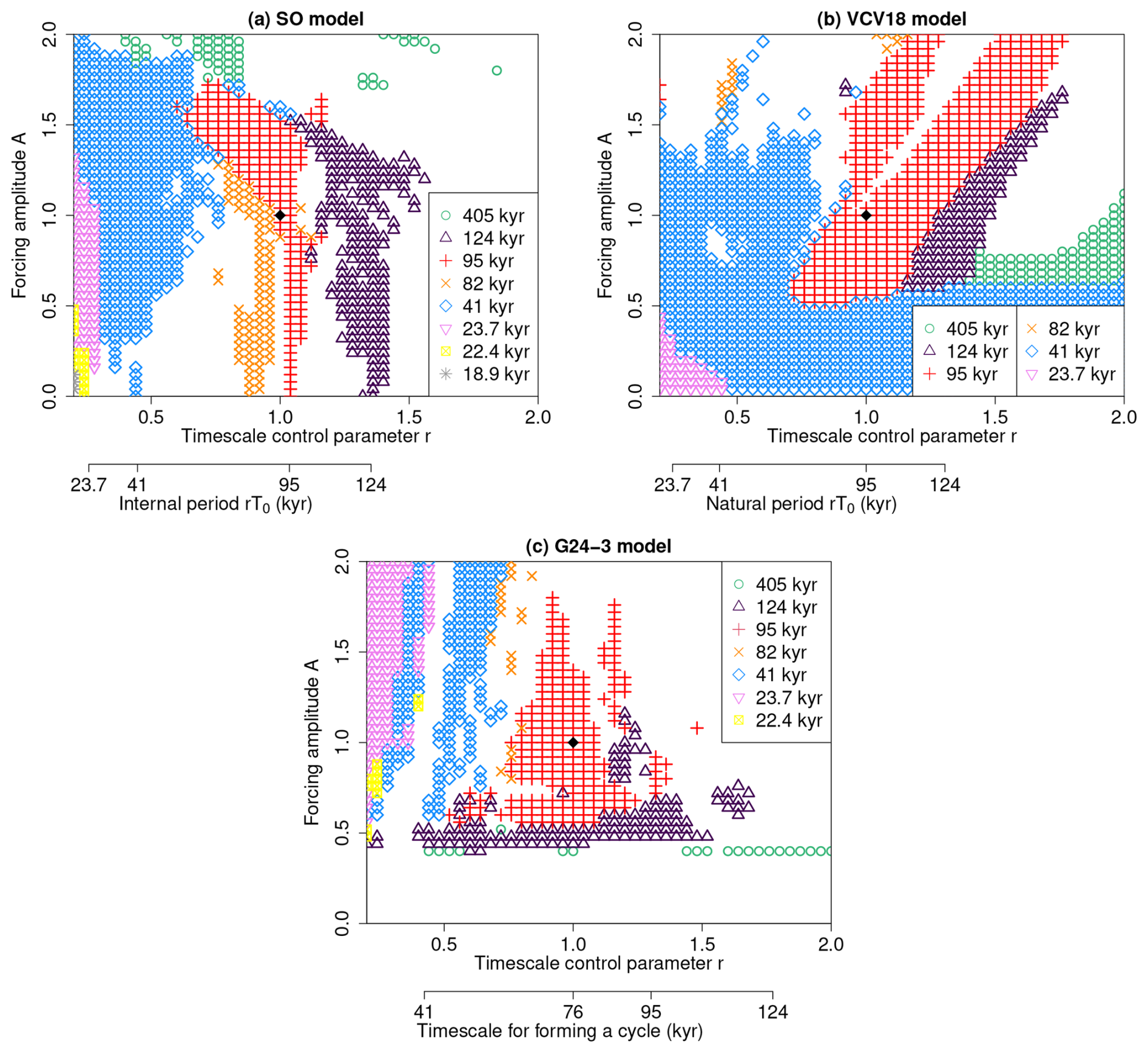
Figure 5 Regime diagram in A–r space. (a) SO model (synchronization mechanism). (b) VCV18 model (nonlinear resonance mechanism in a damped oscillatory system). (c) G24-3 model (nonlinear resonance mechanism in a bistable system with thresholds). The principal period of the simulated dynamics is shown by the symbols in the legend. The most realistic simulations are obtained at A=1 and r=1 (black diamond). A is the forcing amplitude. r is the parameter controlling the timescale of the underlying system. rT₀ is the scaled intrinsic timescale in the SO model and the VCV18 model. In the G24-3 model, the scaled timescale for forming a cycle is $T_{\text{cyc}}\left(r\right)=\mathrm{61.5}r+\mathrm{15}$ kyr.

The VCV18 model does not exhibit quasi-Arnold tongues that touch the horizontal axis at a single point (Fig. 5b). For small but nonzero values of the forcing amplitude A, the principal period is 23.7 kyr when the scaled natural period rT₀ is less than roughly 41 and 41 kyr when rT₀≳41 kyr ($\mathrm{0.5}\lesssim r\le \mathrm{2}$). These correspond to linear responses to the 23 kyr precession and 41 kyr obliquity components of the insolation forcing, respectively. For forcing amplitudes A roughly between 0.5–1.5, three regions appear in succession as the natural period rT₀ varies, each corresponding to a dominant period of 41, 95, and 124 kyr, respectively (Fig. 5b). In each region, the corresponding Q parameter reaches its maximum, confirming that these are resonance phenomena (Fig. 6b). Moreover, the 95 and 124 kyr resonance regions incline toward larger values of rT₀ as A increases, respectively (Fig. 5b). Such a shift in the natural period rT₀ that yields the maximum amplitude is characteristic of nonlinear resonance (Rajasekar and Sanjuan, 2016; Marchionne et al., 2018). Near the realistic forcing amplitude of A≃1, resonances at 41, 95, and 124 kyr emerge when the scaled natural period rT₀ approaches these respective timescales (Figs. 5b and 6b). This correspondence indicates that resonance is driven by a timescale match between the system's natural period and an astronomical period, in line with the classical concept of resonance. We therefore conclude that the proximity between the system's intrinsic timescale and the 95 kyr eccentricity period is crucial for producing the 95 kyr cycles in the VCV18 model as well. Note that the close numerical match between the natural period T₀=95 kyr and the 95 kyr eccentricity period is purely coincidental, and the resonance at 95 kyr can occur for a range of natural periods, $\mathrm{83}\le r{T}_{\mathrm{0}}\le \mathrm{118}$ kyr, for the realistic astronomical forcing A=1.

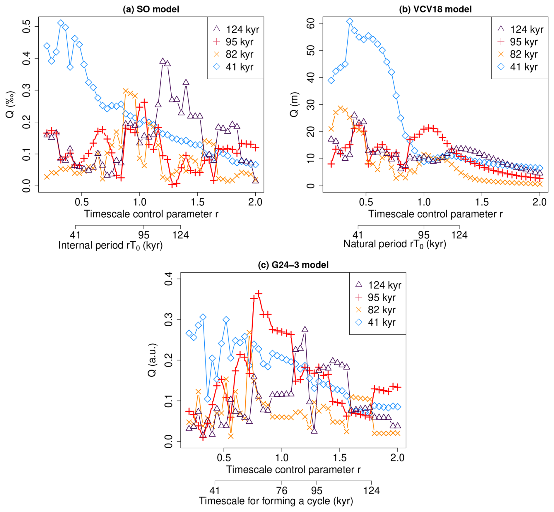
Figure 6 Q spectrum as a function of the timescale control parameter r. (a) SO model (synchronization mechanism). (b) VCV18 model (nonlinear resonance mechanism in a damped oscillatory system). (c) G24-3 model (nonlinear resonance mechanism in a bistable system with thresholds). The most realistic simulations are obtained at r=1, where Q₉₅ for the 95 kyr period is maximal. rT₀ is the scaled intrinsic timescale in the SO model and the VCV18 model. In the G24-3 model, the scaled timescale for forming a cycle is $T_{\text{cyc}}\left(r\right)=\mathrm{61.5}r+\mathrm{15}$ kyr.

In the G24-3 model, as shown in Fig. 5c, 124 kyr glacial cycles as well as 405 kyr cycles occur for a wide range of r, i.e., virtually regardless of the scaled timescale for forming a cycle, T_cyc(r). The 95 kyr cycles also occur for a wide range of scaled timescales T_cyc(r) if A is around 0.6. However, the range of T_cyc(r) giving the 95 kyr cycles is limited to $\mathrm{66}\lesssim T_{\text{cyc}}\left(r\right)\lesssim \mathrm{90}$ kyr at the realistic forcing amplitude A=1. Thus, also in the G24-3 model, the intrinsic timescale is key to having the 95 kyr cycles. We calculate the Q parameters also for this model (Fig. 6c). Among others, Q₉₅ corresponding to 95 kyr period takes a maximum near r=1. This demonstrates that the 95 kyr cycles in the G24-3 model are generated via nonlinear resonance.

We note that the closeness between the intrinsic timescale and the 95 kyr eccentricity period not only ensures the ∼100 kyr dominant period of ice age cycles but also enhances the temporal consistency between the simulations and the proxy data, as shown by Pearson's correlation coefficients for varying parameters r and A in Fig. S5 in the Supplement.

4 Discussion

Our sensitivity experiments show that the models' responses can lock into individual or combined astronomical frequencies, depending on their intrinsic timescales (Fig. 5). The locking frequency can also depend on the amplitude of the astronomical forcing (Fig 5b and c). However, under realistic forcing amplitudes, models tend to produce ∼100 kyr cycles when their intrinsic timescales are close to 100 kyr. This reflects a general property of synchronization and nonlinear resonance, observed across many ice age models (Table 1).

Oerlemans (1982)Saltzman and Maasch (1990)Gildor and Tziperman (2000)Crucifix (2012)Mitsui et al. (2015)Ashwin and Ditlevsen (2015)Ganopolski (2024)Verbitsky et al. (2018)Benzi et al. (1982)Parrenin and Paillard (2012)Ganopolski (2024)

Table 1 Intrinsic timescales of models simulating ∼100 kyr glacial cycles. T_SO is the period of a self-sustained oscillation, T_nat is the period corresponding to the natural frequency, and T_cyc is the timescale for forming a threshold-triggered cycle. The asterisks (*) indicate the models explored in this study.

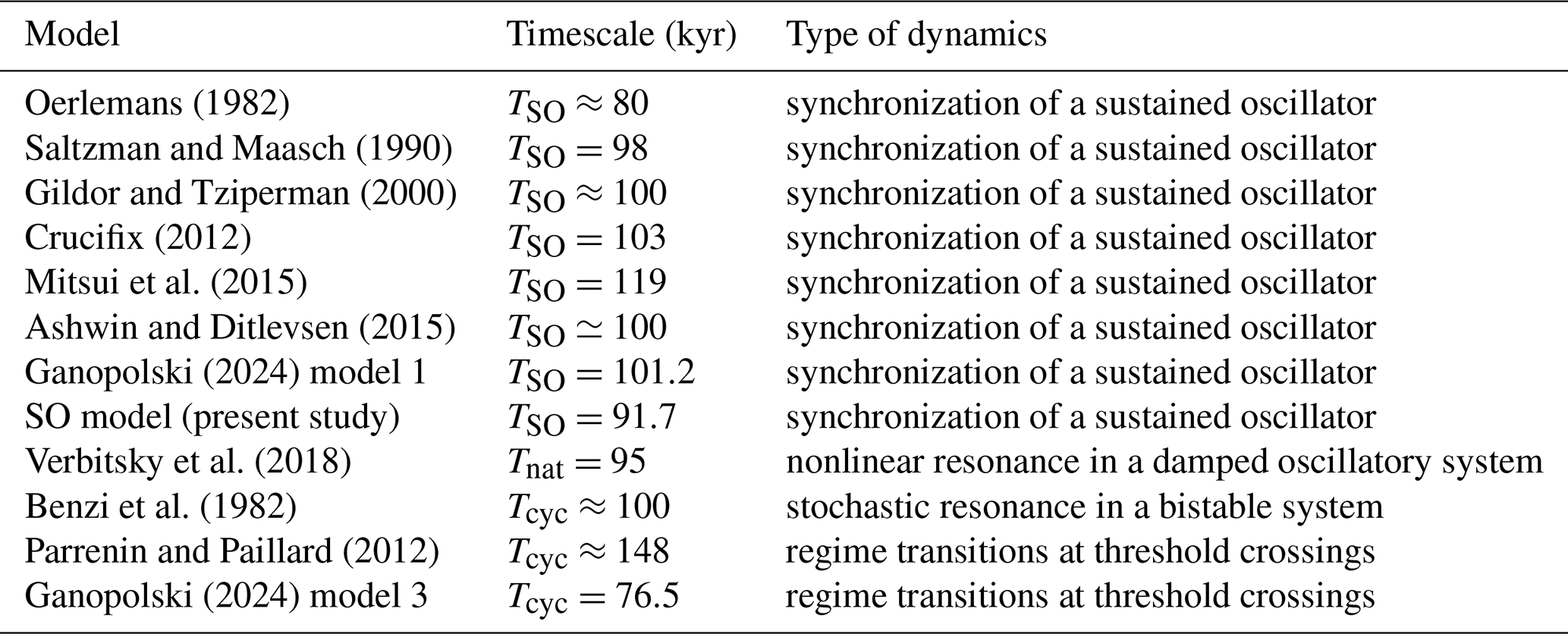
For example, Parrenin and Paillard (2012) simulate glacial cycles using a threshold-based regime-switching model, where the inherent time until the ice increases from v₁=4.5 to v₀=123 m is $(v_{\mathrm{0}}-v_{\mathrm{1}})/{\mathit{\alpha }}_g\simeq \mathrm{126}$ kyr, and the timescale for deglaciation is ${\mathit{\tau }}_{\mathrm{d}}\ln \left|(v_{\mathrm{0}}-{\mathit{\alpha }}_{\mathrm{d}}{\mathit{\tau }}_{\mathrm{d}})/(v_{\mathrm{1}}-{\mathit{\alpha }}_{\mathrm{d}}{\mathit{\tau }}_{\mathrm{d}})\right|\simeq \mathrm{22}$ kyr. Thus, the timescale for forming a cycle is 148 kyr. Although longer than 100 kyr, it is still closer to 100 kyr than 20, 41, or 400 kyr. Benzi et al. (1982) consider noise-induced transitions between wells under weak 100 kyr periodic forcing. In the model, the signal-to-noise ratio is maximal at a certain noise intensity, the so-called stochastic resonance. This occurs when the average waiting time between two noise-induced transitions between the two wells (the inverse of the Kramers rate) is half the forcing period, i.e., ∼50 kyr (Benzi, 2010). Therefore, the intrinsic timescale of a cycle is $\mathrm{2}\times \mathrm{50}=\mathrm{100}$ kyr. The stochastic resonance theory is one of earliest examples treating the ∼100 kyr problem as a matching problem between the Earth's intrinsic timescale and external astronomical timescale. This theory has since been extended to align with Milankovitch theory (Matteucci, 1989; Ditlevsen, 2010). On the other hand, the piecewise linear model by Imbrie and Imbrie (1980) is the example of a model with no 100 kyr scale intrinsic timescale, and it fails to simulate the dominant ∼100 kyr periodicity. Its intrinsic timescales are 42.5 kyr for glaciation and 10.6 kyr for deglaciation.

The models of ∼100 kyr cycles mentioned above are simple conceptual models, but some studies in the literature offer insights on how our timescale-matching hypothesis may hold in more complex models. First, an early study by Oerlemans (1982) demonstrated that an ice-sheet–bedrock system could exhibit 100 kyr scale self-sustained oscillations, especially due to strong feedbacks involving basal melting and sliding of the ice sheets. This model serves as an example in which 100 kyr scale intrinsic oscillations are relevant for producing 100 kyr cycles under insolation forcing, even though our understanding of ice-sheet and lithosphere physics has since been refined. Second, since the G24-3 model was, according to its author, inspired by experiments using the Earth system model of intermediate complexity, CLIMBER-2 model (Ganopolski, 2024), our results obtained from the G24-3 model can be relevant with complex climate systems including carbon cycles and dust–albedo interactions. Mitsui et al. (2023) showed that a version of the CLIMBER-2 model exhibits self-sustained oscillations with periods of several hundred thousand years, due to the glaciogenic dust feedback and carbon cycle feedbacks. Such long timescales are crucial for ∼100 kyr ice age cycles simulated in the CLIMBER-2 model under the forcing.

Although many models have intrinsic timescales around 100 kyr (Table 1), not all have been evaluated from this perspective. The existence of an underlying 100 kyr scale intrinsic timescale is hence our hypothesis based on the finite set of simple models surveyed here.

Different dynamical mechanisms add distinct nuance to the timescale-matching hypothesis. In the synchronization mechanism, the period of glacial cycles closely follows that of self-sustained oscillations, as suggested by the nearly vertical quasi-Arnold tongues (Fig. 5a). In contrast, in the nonlinear resonance mechanism with damped oscillations, the natural period leading to the ∼100 kyr cycles can deviate from 100 kyr, depending on the forcing amplitude, as suggested by the tilted 95 kyr resonance region (Fig. 5b). Thus, this mechanism does not require a precise match between the internal and external periods but rather a general alignment of their timescales. In the case of the bistable model (G24-3), the intrinsic timescale is not purely internal but includes a ∼10 kyr scale lag before favorable astronomical conditions are met. Although these mechanisms differ in their implications, the common factor for the emergence of the ∼100 kyr cycles is the closeness of Earth's intrinsic timescale to the ∼100 kyr periodicity of the eccentricity cycles.

In this study, we distinguished between ice age models that exhibit synchronization and those that exhibit resonance. This distinction can be subtle in some cases. (i) In synchronization theory, the forcing is generally assumed to be small relative to the underlying self-oscillatory dynamics (Pikovsky et al., 2003). If the forcing is strong, it can significantly alter the oscillation amplitude, making it challenging to categorize the phenomenon strictly as either synchronization or resonance. (ii) Excitable systems, which are mono- or multistable in the absence of forcing, can produce repetitive oscillations when subject to small forcing or noise. If the frequency of such excited oscillations becomes locked to astronomical forcing, it resembles synchronization, though synchronization is typically reserved for systems with intrinsic self-sustained oscillations (Pikovsky et al., 2003). Pierini (2023) discusses the 100 kyr cycles from the perspective of a deterministic excitation paradigm and reaches a conclusion similar to ours: that an intrinsic timescale of ∼100 kyr should exist.

In Verbitsky et al. (2018) as well as Daruka and Ditlevsen (2016), the period doubling as well as the period tripling of the 41 kyr periodic cycle is proposed as the scenario to give 100 kyr scale glacial cycles (specifically 82 kyr as well as 123 kyr cycles). This is not inconsistent with the present analysis of the VCV18 model. Indeed, if the VCV18 model is forced by the pure 41 kyr periodic forcing, and if the forcing amplitude is increased, the period-doubling bifurcation is observed as shown in Fig. S6 in the Supplement. Comparing Fig. 5b with Fig. S6, the transition from the 41 kyr regime to the 95 kyr regime in Fig. 5b is considered an analog of a period-doubling bifurcation. The true period doubling is from 41 to 82 kyr. However, the 95 kyr cycles are realized instead of the 82 kyr cycles because the climatic precession forcing, which is modulated by 95 kyr eccentricity cycles, is stronger than the obliquity forcing in the power of the summer solstice insolation at 65° N (Fig. 1e).

Could the timescale-matching hypothesis be extended to the 41 kyr dominant period observed before the Mid-Pleistocene Transition (MPT) (Berends et al., 2021; Legrain et al., 2023)? To address this question, it is important to recall that boreal summer insolation forcing contains only negligible ∼100 kyr power but a strong 41 kyr component. If the 41 kyr glacial cycles are simply linear responses, the intrinsic timescale may be less critical for their realizations. However, if they arise through synchronization or resonance, the intrinsic timescale becomes more relevant, as some models suggest.

In a study using the CLIMBER-2 model, Mitsui et al. (2023) found that 40 kyr scale self-sustained oscillations underlie the 41 kyr response prior to the MPT. In that study, the MPT is attributed to a gradual increase in the period of the self-sustained oscillations from ∼40 kyr to several hundred kyr. Timescale matching is key to the dominant period across the MPT. The G24-3 model exhibits a resonance scenario consistent with the timescale-matching hypothesis, showing shorter intrinsic timescales closer to 41 kyr before the MPT and longer timescales near 76 kyr after the MPT (Fig. S7 in the Supplement). However, the required proximity of the intrinsic timescale to 41 kyr before the MPT depends on the model used. The VCV18 simulates the MPT-like transition if the parameters are changed in time so that the positive-to-negative feedback ratio is increased (Fig. S8a in the Supplement). Over the last 3 Myr, the natural period of damped oscillations increases from ∼75 to 95 kyr, which is calculated from the complex eigenvalue of the Jacobian matrix at the stable state (Fig. S8 in the Supplement). Although the natural period before the MPT (75–80 kyr) is still longer than the observed 41 kyr, this subtle shift is sufficient to produce a 41 kyr periodicity in the VCV18 model. This behavior is already indicated by the 41 kyr region adjacent to the 95 kyr resonance region in Fig. 5b. While models such as CLIMBER-2, G24-3, and VCV18 suggest that long-term parameter changes can shift the intrinsic timescale across the MPT, other models reproduce the MPT-like shift in dominant periodicity without requiring explicit parameter changes (Imbrie et al., 2011; Huybers and Langmuir, 2017; Watanabe et al., 2023). Investigating the relationship between the intrinsic timescale and the 41 kyr response using the present approach requires comparing more models that accurately simulate the records through the MPT. We thus postpone this research to future work.

5 Summary

Determining origin of the ∼100 kyr periodicity in the Late Pleistocene glacial cycles has been an enduring problem in paleoclimate studies. We investigated three simple models of ice age cycles, which produce ∼100 kyr cycles through distinct mechanisms: synchronization of self-sustained oscillations and nonlinear resonance in mono- or multi-stable systems. Although the astronomical forcing possesses only negligible power in the 100 kyr band, these models exhibit ∼100 kyr ice age cycles as a response to the amplitude modulation of climatic precession cycles. This is physically equivalent to a response to the ∼100 kyr eccentricity cycles that modulate climatic precession. Through sensitivity experiments varying the intrinsic timescale of each model, we have revealed that the key factor for the emergence of the ∼100 kyr cycles is the closeness of the Earth's intrinsic timescale to the ∼100 kyr periodicity of the eccentricity cycles, regardless of the specific dynamical mechanism. In other words, the ∼100 kyr period in the astronomical forcing is “selected” because it is close to the intrinsic timescale of the climate system. Note that this is a hypothesis derived from a finite set of models, mostly simple ones. Investigating the intrinsic timescales of more complex models is challenging. If adjusting the timescale of a model proves difficult, artificially varying the astronomical frequencies and observing the response could be a useful approach for evaluating the validity of the timescale-matching hypothesis in complex models.

Appendix A: Power spectral density method

The power spectral density (PSD) S(f) of a time series is estimated using the periodogram (Bloomfield, 2013), which is computed with the R function spec.pgram (R Core Team, 2020). By default, this function applies a split cosine bell taper to 10 % of the data at both the beginning and the end of the time series to minimize discontinuity effects between the start and end of the series. To increase the number of frequency bins in the periodogram, zeros are added to the end of the series to extend its length by a factor of 10 (i.e., pad=9 in the spec.pgram option). Zero padding does not fundamentally affect the PSD of the signal, but the frequency corresponding to a PSD peak is estimated with a higher resolution.

Appendix B: van der Pol–Duffing–Hill equation

We assume that the glacial cycles can be represented by a forced van der Pol–Duffing–Hill equation:

$$\begin{array}{ll}{\displaystyle }& {\displaystyle }\ddot{x}+(\mathit{\mu }{x}^{\mathrm{2}}-\mathit{\kappa })\dot{x}+\mathit{\alpha }x+\mathit{\beta }{x}^{\mathrm{3}}+\mathit{\theta }\\ \text{(B1)}& {\displaystyle }& {\displaystyle }+(\mathit{\nu }+\mathit{\rho }x)I\left(t\right)+\mathit{\eta }{I}^{\mathrm{2}}\left(t\right)=\mathrm{0},\end{array}$$

where the parameters are denoted by Greek letters, and I(t) is an insolation anomaly defined below. Under the restriction to the second-order differential equation, Eq. (B1) is quite comprehensive from the viewpoint of dynamical systems. First, it contains the van der Pol equation $\ddot{x}+(\mathit{\mu }{x}^{\mathrm{2}}-\mathit{\kappa })\dot{x}+\mathit{\alpha }x=\mathrm{0}$, where κ, ν, and α are typically positive (Van der Pol, 1926; Strogatz, 2018). The van der Pol equation is well studied as a generic system showing self-sustained oscillations. Crucifix's group (Crucifix, 2012, 2013; De Saedeleer et al., 2013; Mitsui and Crucifix, 2016) and others (Mitsui and Aihara, 2014; Ashwin et al., 2018) have used the forced van der Pol equation as a mathematical model for investigating ice age dynamics since it can roughly fit the Late Pleistocene glacial cycles.

Second, Eq. (B1) contains the Hill equation $\ddot{x}+[\mathit{\alpha }+\mathit{\rho }I(t\left)\right]x=\mathrm{0}$ if I(t) is periodic in time (Magnus and Winkler, 2004). Furthermore, if I(t) is a simple harmonic, the Hill equation is called the Mathieu equation $\ddot{x}+(\mathit{\alpha }+\mathit{\rho }\cos \mathrm{2}t)x=\mathrm{0}$. The latter is invoked to explain the rhythm of ice age cycles by Rial (1999) from the viewpoint of frequency modulation.

Third, for κ<0, Eq. (B1) contains the Duffing equation $\ddot{x}-\mathit{\kappa }\dot{x}+\mathit{\alpha }x+\mathit{\beta }{x}^{\mathrm{3}}=-\mathit{\nu }I\left(t\right)$ if I(t) is a sinusoid. It is a paradigmatic system of nonlinear resonance as well as chaos (Duffing, 1918; Strogatz, 2018). The Duffing equation exhibits forced oscillations but not self-sustained oscillations. Dropping out the additive forcing and the nonlinear damping term, Eq. (B1) reduces to the model by Daruka and Ditlevsen (2016): $\ddot{x}+a\dot{x}-bx+b{x}^{\mathrm{3}}+bc-bxI\left(t\right)=\mathrm{0},$ where $\dot{x}$ is the global temperature anomaly; x represents a climatic memory effect; and a, b, and c are parameters (different symbols are used in the original reference). Their model is essentially the Duffing–Hill equation since the damping term is linear. A modified version of their model can fit the proxy record well (Riechers et al., 2022).

A way to link Eq. (B1) with a proxy variable of ice age cycles is to make a first-order system taking the so-called Liénard variable $y=\dot{x}-\mathit{\kappa }x+\frac{\mathit{\mu }}{\mathrm{3}}{x}^{\mathrm{3}}$ (Jackson, 1989; Crucifix, 2012), which yields Eqs. (1) and (2). $y={\mathit{\delta }}^{\mathrm{18}}\text{O}-\mathit{\delta }-\mathrm{4}$ links the variable y with the modeled δ¹⁸O (‰) with an offset δ+4. The variable x is an unobserved climate variable. In association with insolation forcing I(t), x determines whether the system is in a glaciation phase or in a deglaciation phase. The scaled summer solstice insolation anomaly I(t) is defined as $I\left(t\right)\equiv \left(F_{\text{65N}}\right(t)-\mathrm{495.7})/\mathrm{24}$, where F_65N(t) is the summer solstice insolation [Wm⁻²] at 65° N calculated with the solar constant of 1368 Wm⁻² (Fig. 1c) (Laskar et al., 2004; Crucifix, 2016). The nonlinear effect of the insolation, ηI²(t), is included to account for the lower sensitivity of the ice volume in the cold period (Paillard, 1998). The term −ρxI(t) is a multiplicative forcing. Such a multiplicative term can appear, from physical point of view, in the energy balance via albedo effects, the ice-mass balance via temperature–precipitation feedback (Le Treut and Ghil, 1983), and the calcifier–alkalinity model (Omta et al., 2016).

The parameters of the equations are calibrated so as to minimize the mean squared error over the last 1 Myr. The minimization is conducted with the Nelder–Mead method implemented in R function optim (R Core Team, 2020). The resultant parameters are κ=1.0536394044, μ=2.9662458029, α=0.0356079021, β=0.0001000922, θ=0.0180996836, ν=0.0514402004, ρ=0.0189082535, η=0.0049923333, and δ=0.1801349684.