Physical characterization of the boundary separating safe and unsafe AMOC overshoot behavior

The Atlantic Meridional Overturning Circulation (AMOC) is an important tipping element within the climate system as it may collapse due to a changing surface buoyancy forcing. Under scenarios of future greenhouse gas emission reductions, it has been suggested that the AMOC may undergo a safe overshoot. However, this was based on a rather conceptual model limiting the physical characterization of the boundary between safe and unsafe AMOC overshoot behavior. Here, using a fully implicit global ocean model, we investigate the AMOC overshoot behavior under different piecewise linear transient freshwater forcing scenarios. We clarify the physics of the collapse and recovery behavior of the AMOC and show that the potential for a safe overshoot is tightly linked to a delicate balance of salt fluxes in the North Atlantic. More specifically, the sign of the time derivative of the integrated salt content in the northern North Atlantic is identified as an adequate indicator of the type of AMOC overshoot behavior. The insights gained are relevant for informing climate policy strategies regarding emission reductions, highlighting the necessity for thoughtful scenarios to prevent an AMOC collapse.

1 Introduction

A key component of the global ocean circulation is the Atlantic Meridional Overturning Circulation (AMOC), which plays an important role in shaping the climate of the Northern Hemisphere. The AMOC consists of the northward transport of warm surface waters and the southward return flow of colder deep waters (Srokosz and Bryden, 2015; Buckley and Marshall, 2016). The AMOC is affected by density differences arising from heat and freshwater fluxes and has been identified as a tipping element in the climate system (Lenton et al., 2008). Models across the full range of complexity suggest that the AMOC could experience a rapid change of state in response to a gradual change in surface buoyancy forcing (Dijkstra, 2024), highlighting its susceptibility to significant shifts under evolving climate conditions.

The major process that can cause a rapid decline in the present-day AMOC is the salt-advection feedback. If the AMOC weakens, less salt is transported northwards, decreasing the density in the north and further weakening the AMOC. In addition to the salt transport, an AMOC weakening also causes a decrease in northward heat transport. Yet, the restoring timescales of salinity and temperature anomalies (Stommel, 1961) by the atmosphere are different: the atmosphere exerts quite a strong control on the sea surface temperature anomalies, but salinity in the ocean does not affect the freshwater flux. Hence, the positive salt-advection feedback can dominate over the negative heat-advection feedback (Marotzke, 2000).

The point beyond which a tipping element changes state is called a tipping point and can be characterized by the global warming level at which it occurs (Armstrong-McKay et al., 2022). Current climate change affects the forcing of the AMOC by making surface water warmer and less saline due to the addition of fresh water from melting ice – mainly from Greenland – and through increasing precipitation over the North Atlantic. Both of these forcing changes would decrease the meridional buoyancy gradient, weakening the AMOC (Gierz et al., 2015). The assessments of the tipping point thresholds have in part led to the societal aspiration to restrict global warming to low levels such as 2.0 or even 1.5 °C above the pre-industrial period (UNFCCC, 2015). However, current emission levels and measured warming rates suggest that keeping the global warming within these restrictions will be difficult to achieve (Rogelj et al., 2023; Forster et al., 2024).

Our study is motivated by recent results where it is shown, using a conceptual box model, that a global warming threshold may be temporarily exceeded without prompting a drastic change in the AMOC state (Ritchie et al., 2021). We consider this AMOC overshoot problem using a fully implicit global ocean model (described in Sect. 2) for which tipping points can be explicitly determined. This enables a detailed analysis of the underlying physical mechanisms that govern AMOC overshoot behavior. In Sect. 3, we first determine the possible freshwater forcing trajectories that allow a safe overshoot of the varying tipping point rates of freshwater forcing as well as freshwater forcing peaks. Next, the analysis of the physics of the recovery and collapse is presented, where salt balances are monitored over different regions of the Atlantic basin. In Sect. 4, a reduced model of the AMOC behavior near the tipping point is studied to determine the precise boundary in parameter space separating safe from unsafe overshoot behavior. Finally, in Sect. 5, we summarize and discuss the results.

2 Model and methods

The description of the global ocean model used in this study is presented in Weijer et al. (2003) and Dijkstra (2007), to which the reader is referred for full details. The model domain represents the global ocean, using continental geometry as well as bottom topography, with the longitude λ ranging from 0 to 360° and the latitude θ from 85.5° S to 85.5° N on a 96×38 grid. The 12 vertical grid levels are non-equidistant, with the most upper layer having a thickness of 50 m and the lowest of 1000 m. The model has no sea-ice component, and the upper ocean is coupled to a simple energy-balance atmospheric model, in which only the heat transport is taken into account. Both the neglected atmospheric moisture transport and sea-ice and ocean interactions may affect the results below, but these effects are outside the scope of this study.

The description on how parameterizations for mixing, diffusion and convection is implemented is described in De Niet et al. (2007), and patterns for the AMOC and other quantities are shown in Weijer et al. (2003) and Den Toom et al. (2012). We use exactly the same parameter setting and configuration as in Dijkstra (2007). In the AMOC model hierarchy (Dijkstra, 2024), this model is located between idealized multi-basin ocean-only models and EMICs (Earth System Models of Intermediate Complexity). The model is fully implicit in that it uses a Crank–Nicholson time discretization such that at each time step, a large nonlinear algebraic system is solved with a Newton–Raphson method. The advantage of this numerical approach is that also steady states and their linear stability can be determined and hence explicit bifurcation diagrams can be efficiently computed (Wubs and Dijkstra, 2023).

The steady-state solutions of the model vs. parameters are computed as described in Dijkstra and Weijer (2005). Under Levitus restoring conditions for the surface salinity field, first a steady reference solution is determined for standard values of the model parameters. From this solution, the freshwater flux that maintains the Levitus surface salinity field under steady-state conditions, below referred to the Levitus flux $F_S^L$, is diagnosed. Moreover, this reference solution will be the starting solution for all the transient simulations in Sect. 3. Note that the surface integral of $F_S^L$ is zero through salt conservation, which holds up to the accuracy of the Newton–Raphson solver. Next, in addition to $F_S^L$, a freshwater perturbation is prescribed over a region in the North Atlantic with domain $P=\mathit{\left\{}\right(\mathit{\lambda },\mathit{\theta })\in [\mathrm{300}\mathrm{°}\mathrm{E},\mathrm{336}\mathrm{°}\mathrm{E}]\times [\mathrm{54}\mathrm{°}\mathrm{N},\mathrm{66}\mathrm{°}\mathrm{N}\left]\mathit{\right\}}$. The strength of the perturbation is ${\mathit{\gamma }}_A{F}_S^P(\mathit{\lambda },\mathit{\theta })$, where $F_S^P(\mathit{\lambda },\mathit{\theta })=\mathrm{1}$ in the region P and zero outside. The value of γ_A, expressed in Sv (Sverdrup, $\mathrm{1}\mathrm{Sv}={\mathrm{10}}^{\mathrm{6}}{\mathrm{m}}^{\mathrm{3}}{\mathrm{s}}^{-\mathrm{1}}$), controls the amplitude of the freshwater perturbation.

Thus, the total freshwater forcing prescribed is

$$\begin{array}{}\text{(1)}& {\displaystyle }{\displaystyle }{F}_S=F_S^L+{\mathit{\gamma }}_A{F}_S^P-Q,\end{array}$$

where Q is a compensation term determined such that

$$\begin{array}{}\text{(2)}& {\displaystyle }{\displaystyle }\underset{S_{\text{oa}}}{\int }{F}_S\cos \mathit{\theta }\mathrm{d}\mathit{\theta }\mathrm{d}\mathit{\lambda }=\mathrm{0},\end{array}$$

with S_oa being the total ocean–atmosphere surface and the cosine term arising from integration over a spherical surface.

The meridional overturning stream function Ψ, expressed in Sv, is defined as the zonally integrated (from λ_W to λ_E) and vertically accumulated meridional volume transport in depth and latitude coordinates:

$$\begin{array}{}\text{(3)}& {\displaystyle }{\displaystyle }\mathrm{\Psi }(\mathit{\theta },z)=r_{\mathrm{0}}\underset{z}{\overset{\mathrm{0}}{\int }}\underset{{\mathit{\lambda }}_W}{\overset{{\mathit{\lambda }}_E}{\int }}v(\mathit{\lambda },\mathit{\theta },z^{\prime })\cos \mathit{\theta }\mathrm{d}\mathit{\lambda }\mathrm{d}{z}^{\prime },\end{array}$$

where $r_{\mathrm{0}}=\mathrm{6.378}\times {\mathrm{10}}^{\mathrm{6}}$ m is the radius of the Earth. The bifurcation diagram (below) will show the maximum value of Ψ below 500 m depth (Ψ_A) vs. the control parameter γ_A, starting from the reference solution described above for γ_A=0 Sv.

3 Results

The bifurcation diagram of the model is shown as the black curve in Fig. 1b. The reference solution has an AMOC strength of about 11 Sv (smaller than in observations due to the low resolution of the model; Dijkstra, 2007), and with increasing γ_A, the AMOC weakens. This branch of stable steady states ends at a saddle-node bifurcation, located at ${\overline{\mathit{\gamma }}}_A=\mathrm{0.1855}$ Sv, which will be referred to below as the tipping point. A branch of unstable steady states exists for decreasing γ_A and leads to a second saddle-node bifurcation at γ_A=0.054. With increasing γ_A, a stable branch of steady states exists for which the AMOC strength is near zero. Thus, for a freshwater flux between 0.054 and 0.1855 Sv, the AMOC is in a bi-stable regime, with a stable upper branch (representing the present-day AMOC) and a coexisting stable lower branch (representing the “off” (collapsed) AMOC state). Beyond the tipping point, only the lower branch exists. Note that the freshwater transport by the overturning at the southern boundary has a near-zero near γ_A=0.054 (see Fig. 4 in Dijkstra and van Westen, 2024). This bifurcation diagram will be the main reference to study the overshoot behavior of the AMOC where a time-dependent freshwater forcing perturbation γ_A=γ_A(t) (specified in later sections) will be applied.

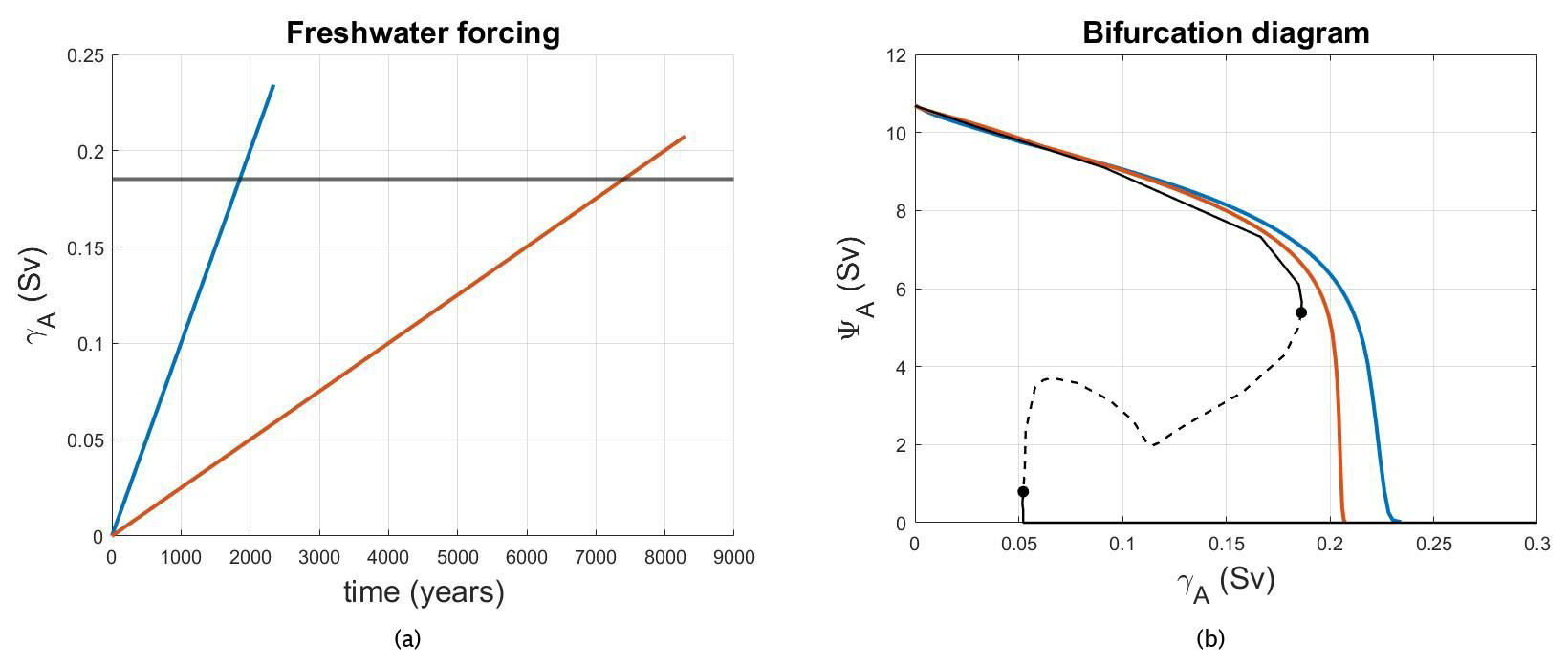
Figure 1 (a) Two linear freshwater forcing trajectories with different slopes are shown as function of time. (b) The AMOC strength curves associated with the forcings in (a) are plotted vs. γ_A in order to be compared to the bifurcation diagram (black curves, with solid (dashed) representing stable (unstable) steady states). The black dots indicate the two saddle-node bifurcations. The horizontal line in (a) corresponds to the tipping point ${\overline{\mathit{\gamma }}}_A=\mathrm{0.1855}$ Sv as shown by the rightmost dot in panel (b).

3.1 Overshoot trajectories

Figure 1b also shows the AMOC response to two cases of transient forcing that overshoot the tipping point ${\overline{\mathit{\gamma }}}_A$. The freshwater forcing grows linearly in time as shown in Fig. 1a where the threshold is denoted by a horizontal line: in one case (blue curve) the forcing goes beyond the tipping point after 900 model years. In the other case (red curve), the tipping point is passed after 7400 model years. In Fig. 1b, the AMOC trajectories of both forcing scenarios initially follow the stable steady-state branch. Since the forcing keeps increasing beyond the tipping point, the AMOC undergoes a change of state. The slower forcing (red) causes the AMOC to stay closer to the steady-state branch, whereas the faster forcing leads to a larger overshoot, making the AMOC reach the off state for higher values of the parameter γ_A.

The AMOC is considered a slow-onset tipping system, which means that crossing a tipping point threshold does not always result in an immediate transition as seen in Fig. 1b. This leaves the possibility that when the freshwater forcing is reversed, the AMOC may undergo a safe overshoot; i.e., it does not collapse (Ritchie et al., 2021). To investigate safe vs. unsafe overshoots of the AMOC, we consider freshwater forcing scenarios γ_A(t) as piecewise linear functions:

$$\begin{array}{}\text{(4)}& {\displaystyle }{\displaystyle }{\mathit{\gamma }}_A\left(t\right)=\left\{\begin{array}{ll}{m}_{\mathrm{1}}t& \mathrm{0}\le t<t_{\mathrm{1}},\\ -m_{\mathrm{2}}t+h& t_{\mathrm{1}}\le t<t_{\mathrm{2}},\\ -m_{\mathrm{2}}{t}_{\mathrm{2}}+h& t\ge t_{\mathrm{2}},\end{array}\right.\end{array}$$

where m₁ and m₂>0 and $h=(m_{\mathrm{1}}+m_{\mathrm{2}})t_{\mathrm{1}}$ is such that γ_A is continuous. Moreover, we chose t₂ such that the forcing after t₂ reaches a constant value, set to be half of the value of the tipping point ${\overline{\mathit{\gamma }}}_A$, i.e.,

$$\begin{array}{}\text{(5)}& {\displaystyle }{\displaystyle }{t}_{\mathrm{2}}=-{\displaystyle \frac{\mathrm{1}}{m_{\mathrm{2}}}}\left({\displaystyle \frac{{\overline{\mathit{\gamma }}}_A}{\mathrm{2}}}-h\right).\end{array}$$

For t<t₁, the forcing represents a linear growth of the freshwater anomaly in the North Atlantic. To have an overshoot beyond the tipping point, the parameters m₁ and t₁ will be chosen such that the maximum value of γ_A (reached at t=t₁) is above the tipping point ${\overline{\mathit{\gamma }}}_A$; hence

$$\begin{array}{}\text{(6)}& {\displaystyle }{\displaystyle }{\mathit{\gamma }}_A\left(t_{\mathrm{1}}\right)=m_{\mathrm{1}}{t}_{\mathrm{1}}=-m_{\mathrm{2}}{t}_{\mathrm{1}}+h>{\overline{\mathit{\gamma }}}_A.\end{array}$$

The subsequent linear decay tries to capture in the simplest way possible the decrease in the freshwater perturbation, which could be faster or slower depending on the effort of society to lower the global emission rates of greenhouse gases.

We investigated three different properties of the freshwater perturbation applied in the region P that can influence the safe or unsafe overshoot of the AMOC: the rate of decline (case A), the rate of increase (case B) and the height of the peak (case C). To understand the physics of the overshoot behavior, only case A, shown in Fig. 2, is needed. The results for the other cases will only be shortly mentioned at the end of Sect. 3.3.

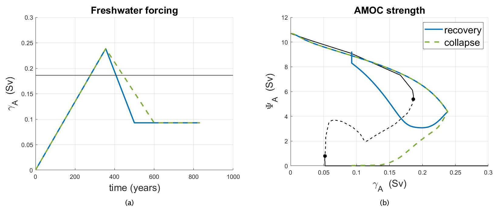
Figure 2 Case A, with (a) the freshwater forcing γ_A(t) and (b) the AMOC strength trajectories. In panel (b) also the bifurcation diagram of the model is again plotted (black curves, with solid (dashed) representing stable (unstable) steady states). The horizontal line in (a) corresponds to the tipping point ${\overline{\mathit{\gamma }}}_A=\mathrm{0.1855}$ Sv as shown by the rightmost dot in panel (b).

Case A represents two scenarios differing only in the rate at which the forcing decreases. The rate m₁ corresponds to $\mathrm{6.0}\times {\mathrm{10}}^{-\mathrm{4}}$ Sv yr⁻¹, which is slightly smaller than the rate of meltwater release from Greenland (about $\mathrm{2.0}\times {\mathrm{10}}^{-\mathrm{3}}$ Sv yr⁻¹ over the period 2002–2021). The two freshwater forcing trajectories of case A (Fig. 2a) reach the same maximum value of 0.2384 Sv but have different decrease rates: $-\mathrm{1.0}\times {\mathrm{10}}^{-\mathrm{3}}$ Sv yr⁻¹ for the blue scenario vs. $-\mathrm{5.7}\times {\mathrm{10}}^{-\mathrm{4}}$ Sv yr⁻¹ for the (dashed) green scenario. Since both trajectories exceed the threshold value ${\overline{\mathit{\gamma }}}_A$, one would expect the AMOC to tip to the off state. However, as can be seen in Fig. 2b, the blue scenario results in a recovery and hence a safe overshoot, while the green one does not. In the safe overshoot scenario, the AMOC spends a shorter time beyond the tipping point (131 years), enabling it to recover. Conversely, in the unsafe overshoot, the AMOC remains beyond the tipping point for a longer time (167 years), and the slower decreasing forcing causes a collapse. In summary, a decrease that is too slow in the forcing prevents a recovery.

3.2 Salt balances

In order to understand the physics underlying the results presented in Sect. 3.1, we consider the integral balance of salinity over the Atlantic basin, with meridional boundaries 𝒮_θ located at 35° S in the south and 60° N in the north. The overall salinity balance is given by Dijkstra (2007):

$$\begin{array}{ll}{\displaystyle }{\mathrm{\Phi }}^{\mathrm{b}}=& {\displaystyle }{\mathrm{\Phi }}^{\mathrm{s}}-{\mathrm{\Phi }}^{\mathrm{a}}\left({\mathit{\theta }}_{\mathrm{s}}\right)+{\mathrm{\Phi }}^{\mathrm{a}}\left({\mathit{\theta }}_{\mathrm{n}}\right)-{\mathrm{\Phi }}^{\mathrm{d}}\left({\mathit{\theta }}_{\mathrm{s}}\right)+{\mathrm{\Phi }}^{\mathrm{d}}\left({\mathit{\theta }}_{\mathrm{n}}\right)\\ \text{(7)}& {\displaystyle }& {\displaystyle }+{\displaystyle \frac{\mathrm{d}}{\mathrm{d}t}}\underset{\text{Atl}}{\int }S\mathrm{d}V.\end{array}$$

Here Φ^s, given by

$$\begin{array}{}\text{(8)}& {\displaystyle }{\displaystyle }{\mathrm{\Phi }}^{\mathrm{s}}=-\underset{{\mathcal{S}}_{\text{oa}}}{\int }{S}_{\mathrm{0}}{F}_S{r}_{\mathrm{0}}^{\mathrm{2}}\cos \mathit{\theta }\mathrm{d}\mathit{\lambda }\mathrm{d}\mathit{\theta },\end{array}$$

represents the (equivalent) salt flux through the ocean–atmosphere surface of the basin (𝒮_oa), positive (negative) when evaporation is larger (smaller) than precipitation; S₀=35 psu indicates the reference salinity. The quantities Φ^a and Φ^d are the advective and diffusive salt fluxes through the boundary 𝒮_θ and are given by

$$\begin{array}{ll}{\displaystyle }& {\displaystyle }{\mathrm{\Phi }}^{\mathrm{a}}\left(\mathit{\theta }\right)=\underset{{\mathcal{S}}_{\mathit{\theta }}}{\int }vS{r}_{\mathrm{0}}\cos \mathit{\theta }\mathrm{d}\mathit{\lambda }\mathrm{d}z,\\ \text{(9)}& {\displaystyle }& {\displaystyle }{\mathrm{\Phi }}^{\mathrm{d}}\left(\mathit{\theta }\right)=-\underset{{\mathcal{S}}_{\mathit{\theta }}}{\int }{K}_{\mathrm{H}}{\displaystyle \frac{\partial S}{\partial \mathit{\theta }}}\cos \mathit{\theta }\mathrm{d}\mathit{\lambda }\mathrm{d}z,\end{array}$$

where K_H is the horizontal diffusivity. The last term on the right-hand side of Eq. (7) measures the changes in time of the salt content stored in the Atlantic basin. This term will be zero for steady states, while it will play an important role in transient solutions. Finally, the residual Φ^b is used to monitor how well the salt balance is closed as in that case it should be zero. It was shown in Dijkstra and van Westen (2024) that the salt balance is closed in the steady case, i.e., along the bifurcation diagram in Fig. 1b.

In the transient situation, we focus first on case A (Fig. 2a and b), where a higher rate of forcing decline results in a recovering AMOC, while a slower decline rate weakens the AMOC until it collapses. Since both scenarios have forcing trajectories with identical peaks at the same time (355 model years), they behave in the same way during the first 355 years. Due to the different rates at which the forcing decreases, we will focus on this phase to characterize the safe and unsafe overshoots. In Fig. 3a, three main contributions of the salt balance are considered: the surface flux Φ^s, the tendency of the integrated salt content, and the net salt flux Φ^lat through the lateral boundaries $S_{{\mathit{\theta }}_{\mathrm{s}}}$ and $S_{{\mathit{\theta }}_{\mathrm{n}}}$, where θ_s=35° S and θ_n=60° N. Here,

$$\begin{array}{}\text{(10)}& {\displaystyle }{\displaystyle }{\mathrm{\Phi }}^{\text{lat}}=\mathrm{\Phi }\left({\mathit{\theta }}_{\mathrm{s}}\right)-\mathrm{\Phi }\left({\mathit{\theta }}_{\mathrm{n}}\right),\end{array}$$

where $\mathrm{\Phi }\left(\mathit{\theta }\right)={\mathrm{\Phi }}^{\mathrm{a}}\left(\mathit{\theta }\right)-{\mathrm{\Phi }}^{\mathrm{d}}\left(\mathit{\theta }\right)$; Φ^lat is positive when salt is transported into the basin. Figure 3b shows the decomposition of the lateral fluxes into advective and diffusive fluxes at the northern and southern boundary of the Atlantic Ocean.

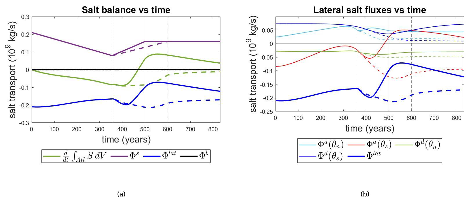
Figure 3 (a) Terms in the integrated salt balance and (b) lateral salt fluxes over the Atlantic basin boundaries along the AMOC trajectories in Fig. 2a and b. In both panels (a) and (b), the solid curves are for the recovery (safe overshoot) scenario and the dashed ones for the collapse (unsafe overshoot) scenario. The vertical lines mark the points when the forcing changes in time: at model year 355, the forcing reaches its peak in both scenarios; at the second vertical line (model year 500), the forcing in the safe overshoot scenario stops decreasing; and at the dashed vertical line (model year 600), the forcing in the unsafe overshoot scenario stops decreasing. In the legend of panel (b), θ_s=35° S and θ_n=60° N.

While γ_A increases, the surface salt flux Φ^s decreases linearly (purple curve in Fig. 3a) due to the input of freshwater in the Atlantic. However, this flux is still positive, which means that there is a net salt buildup in the Atlantic basin that needs to be compensated through salt transport out of the basin. This transport occurs through the lateral boundaries, where (note that Φ^lat is negative) salt is transported out of the basin. Its absolute value is decreasing with increasing γ_A, and hence less salt is transported out through the lateral boundaries. However, since the integrated salt content is decreasing ($\frac{\mathrm{d}}{\mathrm{d}t}{\int }_{\text{Atl}}S\mathrm{d}V<\mathrm{0}$), the lateral salt outflow is larger than that needed to compensate the surface salt input. This implies that the lateral salt transport does not adjust quickly enough to the changing forcing, remaining stronger than needed for a steady balance. An important contribution to the lateral fluxes is due to Φ^a(θ_s) (red curve in Fig. 3b), which indicates the salt was transported northwards at the southern boundary. As Φ^a(θ_s) is negative, the salt is being transported out of the basin. Note that here the flux at the southern boundary dominantly determines the behavior of Φ^lat.

At the time when γ_A starts to decrease, Φ^s increases in both forcing scenarios, reflecting that less freshwater enters the ocean through its surface. At the same time, the dashed curves and the solid ones in Fig. 3a begin to diverge. When γ_A decreases more rapidly (solid curves), the increase in Φ^s is faster (solid purple curve). At the same time, Φ^lat (solid blue curve) reaches a minimum and then starts to increase again, indicating that the amount of salt transported out of the basin is reduced. These two factors make the Atlantic basin saltier as can be seen by the positive $\frac{\mathrm{d}}{\mathrm{d}t}{\int }_{\text{Atl}}S\mathrm{d}V$ (solid green curve): less freshwater is put in and less salt is transported out. In the case of collapse (dashed curves), the combination of freshwater input and salt transport outwards does not make the term $\frac{\mathrm{d}}{\mathrm{d}t}{\int }_{\text{Atl}}S\mathrm{d}V$ positive: the salt flux through the lateral boundaries remains too strong to balance the slow increase in Φ^s and hence the salt storage in the Atlantic keeps decreasing.

To explain the different behavior of the two scenarios in more detail, two boxes are defined: one in the North Atlantic and one in the South Atlantic. The northern box spans latitudes from 40 to 60° N and the southern one extends from 15 to 35° S. Both are bounded zonally by the land bordering the Atlantic. We compute the box-averaged densities ρ_i, salinities S_i and temperatures T_i ($i=\mathrm{s},\mathrm{n}$) by integrating over the total volume of each box. The location of the southern box has been motivated by earlier work (Rahmstorf, 1996), showing a linear relation between the AMOC strength and the meridional density difference. The meridional density difference $\mathrm{\Delta }\mathit{\rho }:={\mathit{\rho }}_{\mathrm{n}}-{\mathit{\rho }}_{\mathrm{s}}$ is shown in Fig. 4a together with the AMOC strength. The density difference behaves in the same way in the two scenarios up to the point where the freshwater forcing reaches its peak. Afterwards, the different decrease rates lead to changes in Δρ. In the collapse case, Δρ keeps decreasing, while it has a minimum when the AMOC recovers after the overshoot. As shown in Fig. 4b, Δρ is well correlated with the AMOC strength, consistent with other low-resolution ocean model studies (Rahmstorf, 1996) and a consequence of the thermal wind balance. In the case of collapse, the density is plotted vs. the AMOC strength for the whole time of the simulation, while in the recovery case, the relation is linear only during the increase in the forcing; in the period of the forcing decrease the AMOC has a more complex, time-dependent response (not shown).

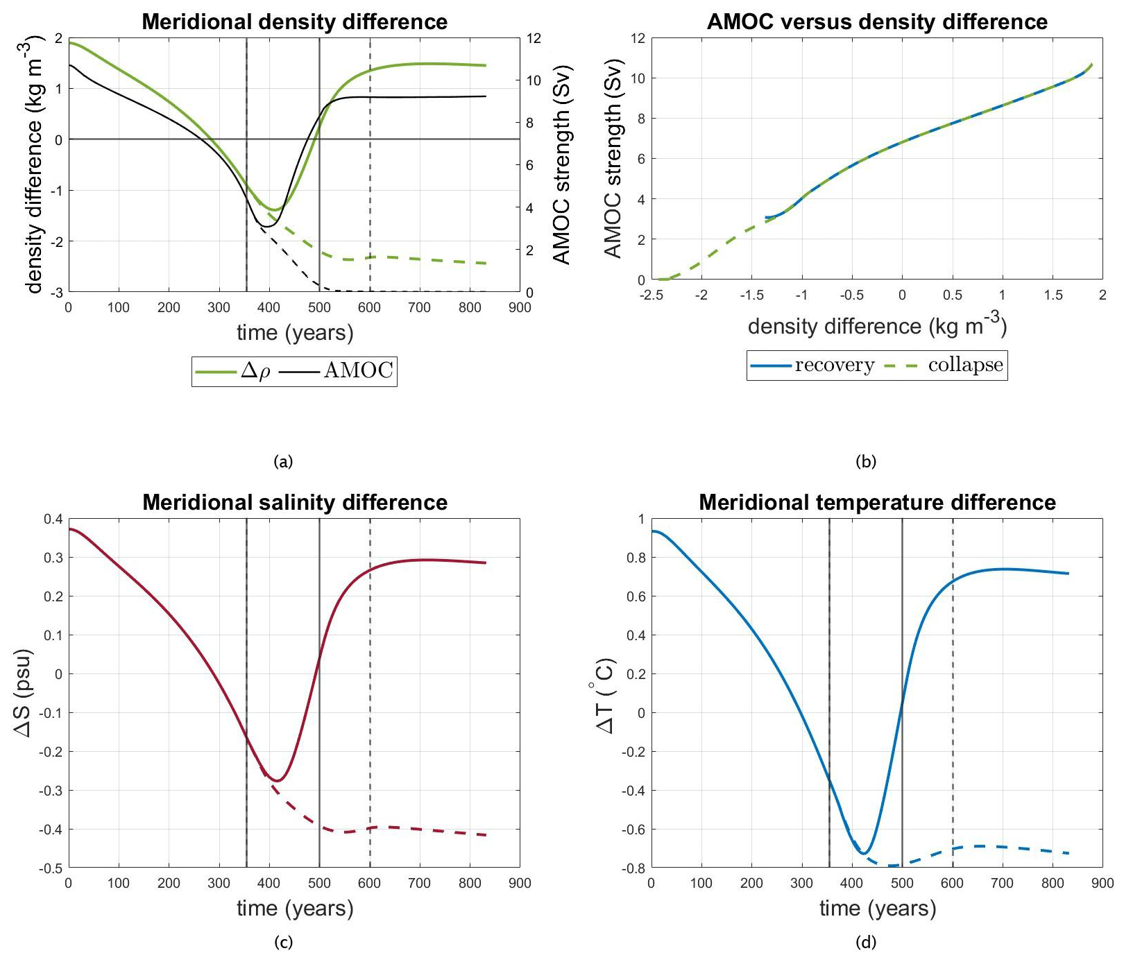
Figure 4 Diagnostics of changes in the northern and southern boxes associated with Fig. 2a and b. (a) The meridional density difference and the AMOC strength are plotted vs. time. (b) The relation between Δρ and the AMOC strength. Box-averaged density contribution of (c) meridional salinity (α_SΔS) and (d) temperature differences (α_TΔT). The solid curves are for the safe overshoot scenario and the dashed ones for the unsafe overshoot scenario. The vertical lines mark the points when the forcing changes.

We further decompose the density difference contribution by salinity (ΔS) and temperature (ΔT) meridional differences in Fig. 4d and c. Note that ΔT has a smaller impact on Δρ compared to ΔS because the thermal expansion coefficient ${\mathit{\alpha }}_T={\mathrm{10}}^{-\mathrm{4}}{{\mathrm{C}}^{\mathrm{°}}}^{-\mathrm{1}}$ is smaller than the haline contraction coefficient ${\mathit{\alpha }}_S=\mathrm{7.6}\times {\mathrm{10}}^{-\mathrm{4}}{\mathrm{psu}}^{-\mathrm{1}}$ used in the linear equation of state. An increasing amount of freshwater is being introduced into the northern region of the Atlantic Ocean, which decreases the salinity difference (ΔS) between the northern and southern boxes until it reaches 0 psu at around 300 model years. After that point until t=t₁ (when the forcing stops increasing) ΔS keeps decreasing, becoming more negative. The salinity in the north changes more than in the south (not shown), not only in range (in the north, it spans a range between 0.65–0.85 psu depending on the scenario while only a range of around 0.1 psu in the south) but especially in shape. The main contribution to ΔS results from changes in the northern box. This is not surprising given the northern location of the prescribed freshwater input anomaly γ_A. The freshwater anomaly is weakening the AMOC, which results in a reduced meridional heat transport northward. This cooling effect in the northern region makes ΔT smaller. The northern temperature spans a range almost 4 times as big as the one in the south in the safe overshoot scenario and 9 times as big as in the unsafe overshoot one; hence the main contribution to ΔT comes from the northern box. In the safe overshoot scenario (solid lines), ΔT and ΔS hit their lowest value before rising again, eventually stabilizing at a positive value. Conversely, in the unsafe overshoot scenario, both ΔS and ΔT continue to decline. In the collapsed state, the northern regions become less saline and cooler than the southern regions.

3.3 Physics of safe/unsafe overshoot

As most density changes occur in the northern box, we apply the salt balance (Eq. 7) to the northern box that extends over the Atlantic basin from 40 to 60° N. The values of the fluxes in the northern region (Fig. 5a) show that, unlike in the whole Atlantic basin case, there is a net freshwater input (Φ^s<0) through the surface and a net saline water input through lateral boundaries. When γ_A starts to decrease, the response of the northern box reveals the precise mechanism of the AMOC safe/unsafe overshoot. In the safe overshoot scenario, a faster decline in freshwater forcing allows the lateral salt transport to surpass the effect of the freshwater input. This results in the change in sign of the tendency of the integrated salt content from negative to positive. Consequently, the northern box experiences an increase in salinity, reinforcing the AMOC and promoting its recovery. In contrast, in the unsafe overshoot scenario, the freshwater forcing remains dominant over the lateral salt transport, leading to a persistent net loss in salt storage $(\frac{\mathrm{d}}{\mathrm{d}t}{\int }_{\text{northbox}}S\mathrm{d}V<\mathrm{0})$. This results in a further freshening of the northern box and in a consequent decrease in ΔS and Δρ, which keeps weakening the AMOC and drives it toward a collapse. A detailed examination of the lateral fluxes within the northern box, shown in Fig. 5b, reveals that the advective salt transport through its southern boundary of this box is the dominant flux. This advective flux, which transports saline waters northwards, plays a crucial role in compensating the surface freshwater perturbation and thereby influences the AMOC behavior under different forcing scenarios.

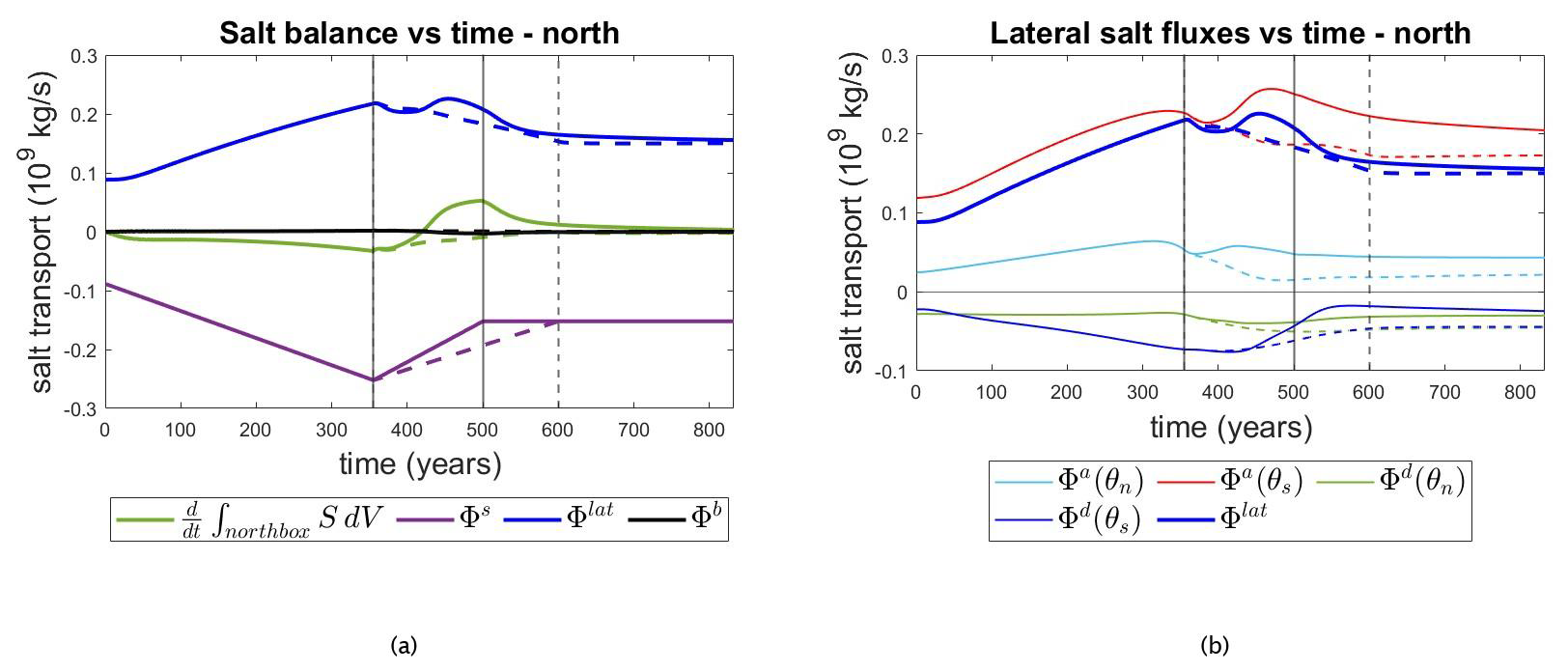
Figure 5 (a) Terms in the integrated salt balance and (b) lateral salt fluxes over the northern box along the AMOC trajectories in Fig. 2a and b. In both panels (a) and (b), the solid curves are for the recovery case and the dashed ones for the collapse. The vertical lines mark the points when the forcing changes. In the legend of panel (b), θ_s=40° N and θ_n=60° N.

Salt balance computations were similarly performed for the southern box but the corresponding plots have been omitted, as the salt fluxes in the South Atlantic have a negligible impact on the AMOC recovery dynamics. In the South Atlantic, the range of the freshwater anomaly is approximately an order of magnitude lower – of magnitude about 20 times less – than that computed in the North Atlantic, making its influence on the recovery or collapse minimal. Moreover, the lateral salt fluxes exhibit a smaller range as well, being roughly 11 times smaller than in the AMOC collapse scenario and 4 times smaller than in the safe overshoot scenario in comparison to their North Atlantic counterparts. Therefore, the essence of the mechanism can be found in the interplay between lateral salt transport and freshwater input in the northern box. It is the relatively early overcoming of freshwater surface flux by lateral salt transport that characterizes the recovery phase of the AMOC. This is quantitatively reflected in the shift from a negative to a positive time derivative of the integrated salt content, a change that signals the key transition in the dynamics. The Atlantic basin, particularly its northern regions, begins to retain more salt, thereby restoring the meridional salinity (and density) gradients crucial for maintaining the AMOC.

The same analysis done for case A was applied to two other cases (B and C). For case B, two freshwater forcing trajectories reach the same maximum value of 0.235 Sv but at different rates. The forcing then decreases linearly at the same rate in both scenarios. The slower increasing forcing causes a collapse, while the faster increasing forcing allows a recovery. As in case A, the AMOC is unable to recover when it has a more prolonged exposure to forcing levels beyond the tipping point. This makes the time spent beyond the tipping point an important factor that influences whether the AMOC collapses or recovers, as was also shown in Ritchie et al. (2021) using a conceptual box model. In case C, both forcing trajectories have the same rate of increase, but now they differ in terms of maximum values of γ_A(t). One peaks after 350 years, while the other reaches a higher peak above the threshold after 370 years. They both get to the same fixed level after 600 years, which means that the rate at which their decrease is different. The lower peak forcing leads to a weaker AMOC decrease and a subsequent recovery, while the higher forcing makes the AMOC tip to the off state. In both cases, the same mechanism as in case A is responsible for causing the safe/unsafe overshoot behavior.

4 Mathematical analysis of limiting cases

The aim of this section is to study the transient solutions of AMOC behavior analytically using a reduced mathematical model. The dynamics of the AMOC strength, indicated by x, can be approximated near a saddle-node bifurcation (which we know exists in the global ocean model used in Sect. 3) by the following (Li et al., 2019) non-autonomous ordinary differential equation (ODE):

$$\begin{array}{}\text{(11)}& {\displaystyle }{\displaystyle \frac{\mathrm{d}x}{\mathrm{d}\mathit{\tau }}}=-x^{\mathrm{2}}-f\left(\mathit{\tau }\right),\end{array}$$

where the forcing is a piecewise linear function:

$$\begin{array}{}\text{(12)}& {\displaystyle }{\displaystyle }f\left(\mathit{\tau }\right)=\left\{\begin{array}{ll}-\mathit{\alpha }(\mathrm{1}-\mathit{\tau })& {\mathit{\tau }}_{\mathrm{0}}<\mathit{\tau }<{\mathit{\tau }}_{\mathrm{1}},\\ \mathit{\beta }(\mathrm{1}-\mathit{\tau })+k& \mathit{\tau }>{\mathit{\tau }}_{\mathrm{1}},\end{array}\right.\end{array}$$

with $\mathit{\alpha },\mathit{\beta }>\mathrm{0}$ and $k=(\mathit{\alpha }+\mathit{\beta })({\mathit{\tau }}_{\mathrm{1}}-\mathrm{1})$ to make the forcing continuous.

The advantage of considering the above one-dimensional model is that analytical solutions can be determined. Using this framework, we will be able to determine a priori the rate of decline in forcing – given a fixed peak and rate of increase – that allows the AMOC to achieve a safe overshoot. Finally, we will compare these analytical findings with the numerical results obtained from the global ocean model.

4.1 Local form near the saddle-node bifurcation

To be able to compare with the ocean model later in Sect. 4.4, we need to use the general form of the saddle-node bifurcation

$$\begin{array}{}\text{(13)}& {\displaystyle }{\displaystyle \frac{\mathrm{d}X}{\mathrm{d}t}}=a{X}^{\mathrm{2}}+bX+c-\mathit{\gamma }\left(t\right),\end{array}$$

where γ(t) is defined as in Eq. (4). In order to get the equation in the form of Eq. (11), a rescaling is needed. We thereby apply the following change of variables:

$$\begin{array}{}\text{(14)}& {\displaystyle }{\displaystyle }\left\{\begin{array}{l}x=-a{t}_{\text{tip}}\left(X+\frac{b}{\mathrm{2}a}\right),\\ \mathit{\tau }=\frac{t}{t_{\text{tip}}},\\ \mathit{\alpha }=-a{m}_{\mathrm{1}}{t}_{\text{tip}}^{\mathrm{3}},& \mathit{\beta }=-a{m}_{\mathrm{2}}{t}_{\text{tip}}^{\mathrm{3}},\end{array}\right.\end{array}$$

with $t_{\text{tip}}=\frac{c}{m_{\mathrm{1}}}-\frac{b^{\mathrm{2}}}{\mathrm{4}a{m}_{\mathrm{1}}}$. Rewriting Eq. (13) as

$${\displaystyle \frac{\mathrm{d}X}{\mathrm{d}t}}=a{\left(X+{\displaystyle \frac{b}{\mathrm{2}a}}\right)}^{\mathrm{2}}+\left(c-{\displaystyle \frac{b^{\mathrm{2}}}{\mathrm{4}a}}\right)-\mathit{\gamma }\left(t\right),$$

we can substitute the new variables and get
for $t\in [t_{\mathrm{0}},t_{\mathrm{1}}]$

$$\begin{array}{ll}{\displaystyle \frac{\mathrm{d}x}{\mathrm{d}\mathit{\tau }}}& {\displaystyle }={\displaystyle \frac{\mathrm{d}x}{\mathrm{d}t}}{\displaystyle \frac{\mathrm{d}t}{\mathrm{d}\mathit{\tau }}}=t_{\text{tip}}{\displaystyle \frac{\mathrm{d}x}{\mathrm{d}t}}\\ {\displaystyle }& {\displaystyle }=t_{\text{tip}}\left(-a\cdot t_{\text{tip}}\right){\displaystyle \frac{\mathrm{d}X}{\mathrm{d}t}}=-a{t}_{\text{tip}}^{\mathrm{2}}{\displaystyle \frac{\mathrm{d}X}{\mathrm{d}t}}\\ {\displaystyle }& {\displaystyle }=-x^{\mathrm{2}}+\mathit{\alpha }(\mathrm{1}-\mathit{\tau }).\end{array}$$

For t>t₁, similar calculations lead to

$${\displaystyle }{\displaystyle \frac{\mathrm{d}x}{\mathrm{d}\mathit{\tau }}}=-x^{\mathrm{2}}-\mathit{\beta }(\mathrm{1}-\mathit{\tau })-k.$$

In this way, the problem is in the form of Eq. (11).

4.2 Analytical solution

Analytical solutions to Eq. (11) can be found in terms of Airy functions (Li et al., 2019). We first compute the bifurcation diagram of the corresponding autonomous system assuming τ as the bifurcation parameter (instead of time). The steady states are given by

$$\begin{array}{}\text{(15)}& {\displaystyle }{\displaystyle }{x}^{\pm }\left(\mathit{\tau }\right)=\pm \sqrt{-f\left(\mathit{\tau }\right)},\end{array}$$

or more explicitly $x_{\mathrm{1}}^{+}\left(\mathit{\tau }\right)=\sqrt{\mathit{\alpha }(\mathrm{1}-\mathit{\tau })}$, $x_{\mathrm{1}}^{-}\left(\mathit{\tau }\right)=-\sqrt{\mathit{\alpha }(\mathrm{1}-\mathit{\tau })}$, $x_{\mathrm{2}}^{+}\left(\mathit{\tau }\right)=\sqrt{-\mathit{\beta }(\mathrm{1}-\mathit{\tau })-k}$ and $x_{\mathrm{2}}^{-}\left(\mathit{\tau }\right)=-\sqrt{-\mathit{\beta }(\mathrm{1}-\mathit{\tau })-k}$. The functions $x_i^{\pm }\left(\mathit{\tau }\right),i=\mathrm{1},\mathrm{2}$ form two parabolas which represent the bifurcation diagram. When a full solution of Eq. (11) crosses one of these curves, its derivative becomes zero, which means that $x_i^{\pm }\left(\mathit{\tau }\right)$, $i=\mathrm{1},\mathrm{2}$ separate regions in the phase plane (t,x) where the derivative has different signs. Following the same methodology as in Li et al. (2019), the solution x(τ) is given in the Appendix.

Figure 6a shows two examples of forcing that differ in the value of β, and Fig. 6b shows the associated solutions. Continuous solutions as the one in blue reproduce the recovery of the AMOC, while the solutions with a vertical asymptote (in red) are the collapses. The bifurcation diagram for both cases (treating τ as parameter) is also shown as the thin curves. As the analytical approximation is tailored for a neighborhood of a single saddle-node bifurcation, it excludes the off state of the AMOC. Consequently, the post-collapse behavior cannot be captured within this analytical framework.

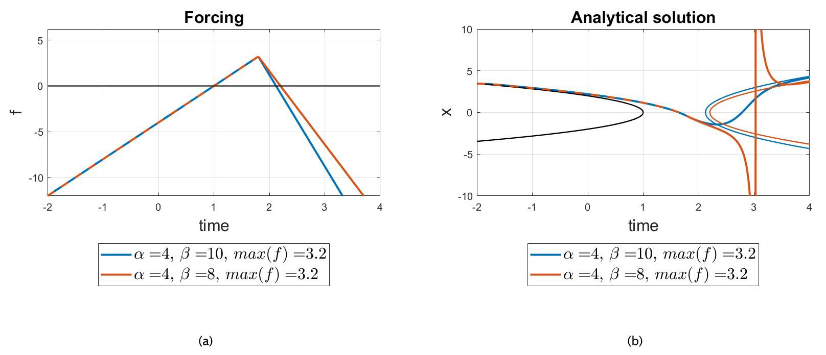
Figure 6 (a) Piecewise linear forcing that increases for $\mathit{\tau }<{\mathit{\tau }}_{\mathrm{1}}=\mathrm{1.8}$ and decreases for τ>τ₁. The rate of decrease is different in the two cases: β=10 for the blue curve, β=8 for the red one and α=4 for both cases. (b) Analytical solution of Eq. (11) given the forcing in (a). The blue curve is a safe overshoot and the red one an unsafe one. The parabolas refer to the fixed points for constant τ, following Eq. (15).

4.3 Conditions for a safe overshoot

Given that the main scenarios analyzed in Sect. 3 are the ones of case A, we focus here on studying conditions for a safe overshoot in the case of a fixed value of α. We pick α=84 for reasons that will become clear in Sect. 4.4 below. First of all, the solution in the time interval with an increasing forcing ($\mathit{\tau }\in [{\mathit{\tau }}_{\mathrm{0}},{\mathit{\tau }}_{\mathrm{1}}]$) has a collapse time at $\mathit{\tau }={\mathit{\tau }}^{*}$, meaning that the solution reaches −∞. The value of τ^* depends on the parameter α, and it is given by the asymptote of the pullback attractor, which can be explicitly computed: ${\mathit{\tau }}^{*}\left(\mathit{\alpha }\right)=\mathrm{1}+\mathrm{2.338}{\mathit{\alpha }}^{-\mathrm{1}/\mathrm{3}}$ (Li et al., 2019). This scenario corresponds to a prolonged increasing forcing that makes the AMOC collapse before the forcing starts decreasing. To avoid this kind of unsafe overshoot, we need ${\mathit{\tau }}^{*}\notin [{\mathit{\tau }}_{\mathrm{0}},{\mathit{\tau }}_{\mathrm{1}}]$, i.e.,

$$\begin{array}{}\text{(16)}& {\displaystyle }{\displaystyle }{\mathit{\tau }}_{\mathrm{1}}<{\mathit{\tau }}^{*}\left(\mathit{\alpha }\right).\end{array}$$

From now on, we make sure that the condition in Eq. (16) is satisfied and the solution is continuous on the interval [τ₀,τ₁]. For α=84, this means that the forcing must have its peak before τ=1.5453.

Solutions for different values of τ₁ and β are computed, and a fraction of those is shown in Fig. 7a and b. For the values of (τ₁,β) for which a collapse happens, the collapse time τ^* is computed (where $\mathit{\tau }={\mathit{\tau }}^{*}$ is the equation of the asymptote). For each value of τ₁, Fig. 7c displays the collapse times τ^* as a function of the rate of decline β of the forcing. As anticipated, a smaller value of β corresponds to a smaller τ^*. This indicates that as the forcing decreases more rapidly, the collapse is postponed, and if the decline is sufficiently fast, the collapse can be entirely avoided.

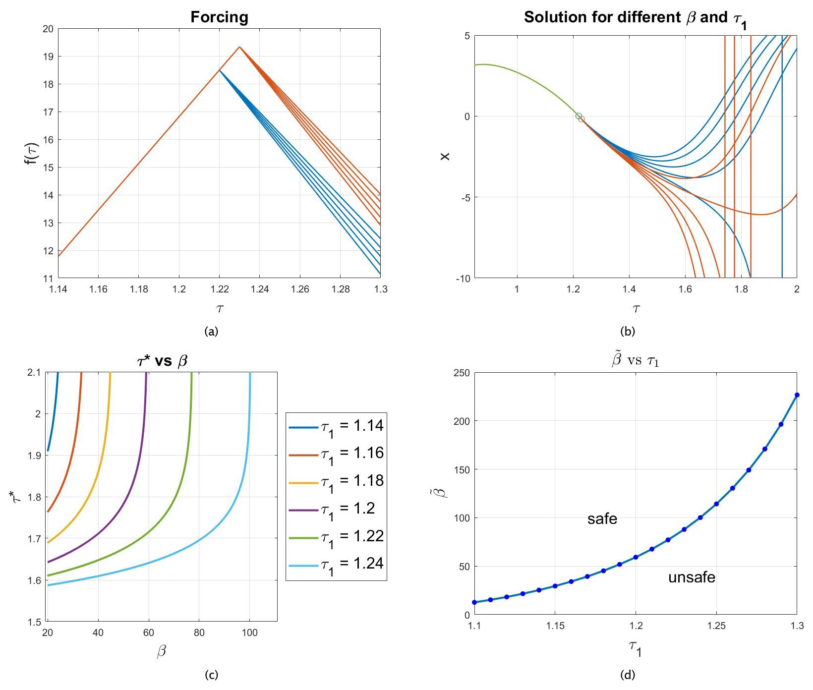
Figure 7 (a) Forcing and (b) associated solutions to Eq. (11). The values of the parameters are α=84, τ₁=1.22 (in red), τ₁=1.23 (in blue) and $\mathit{\beta }\in [\mathrm{92},\mathrm{76}]$. (c) Collapse time τ^* vs. decline rate β of the forcing f(τ) for α=84 and different values of τ₁ between 1.14–1.24. (d) The maximum value of β ($\stackrel{\mathrm{̃}}{\mathit{\beta }}$) for which the solution collapses vs. the time τ₁ at which the forcing reaches its peak. This critical curve separates the safe and unsafe overshoot regions in the parameter space $({\mathit{\tau }}_{\mathrm{1}},\stackrel{\mathrm{̃}}{\mathit{\beta }})$ for α=84.

Finally, for each τ₁ we can take the largest value of β, say $\stackrel{\mathrm{̃}}{\mathit{\beta }}$, for which the solution exhibits a collapse. For all $\mathit{\beta }<\stackrel{\mathrm{̃}}{\mathit{\beta }}$, the forcing is decreasing in a slower way and hence all the associated solutions collapse. On the other hand, for all $\mathit{\beta }>\stackrel{\mathrm{̃}}{\mathit{\beta }}$, the solutions recover. Thus, the curve (${\mathit{\tau }}_{\mathrm{1}},\stackrel{\mathrm{̃}}{\mathit{\beta }}\left({\mathit{\tau }}_{\mathrm{1}}\right))$, plotted in Fig. 7d for α=84, divides the parameter space into safe and unsafe overshoot regions. The value of $\stackrel{\mathrm{̃}}{\mathit{\beta }}$ decreases as τ₁ decreases. In fact, given that α is fixed, a smaller τ₁ corresponds to a lower peak of the forcing, which in turn leads to a smaller decline in the AMOC. This allows for a longer AMOC overshoot (hence a slower decrease in the forcing) while still having a recovery. The analytic solutions provide a clear picture of the response of the AMOC to the freshwater forcing taking into account the rate of the forcing decrease β and time τ₁ when the forcing begins to decrease (in the same way one could take the peak value of the forcing, as was done in the analysis of case C in Sect. 3). Hence, within this simple analytical framework, a critical curve has been found defining stability regions similar to that in the conceptual model used in Ritchie et al. (2021).

4.4 Connection to the global ocean model: case A

We now compare the results obtained from the simple ODE in Eq. (11) with the numerical simulations obtained with the global ocean model for which results are presented in Sect. 3. A quadratic fit is made near the tipping point in the bifurcation diagram (Fig. 1b) where Ψ_A is computed as a function of the bifurcation parameter γ_A. Hence, the AMOC strength Ψ_A=X is used as the primary variable in Eq. (13) and the fit to determine the constants a, b and c yields $a=-\mathrm{0.0060},b=\mathrm{0.0658}$ and c=0.0056. In order to have recovery and collapse simulations while staying as close as possible to the saddle-node bifurcation, results for four additional global ocean model simulations (labeled a–d) are shown in Fig. 8a and b. They all have $m_{\mathrm{1}}=\mathrm{6.1972}\times {\mathrm{10}}^{-\mathrm{4}}$ Sv yr⁻¹ and γ(t₁)=0.22 Sv (with t₁=355 years), while they differ for the value of $m_{\mathrm{2}}=\mathit{\{}\mathrm{8.7},\mathrm{3.7},\mathrm{2.3},\mathrm{1.1}\mathit{\}}\times {\mathrm{10}}^{-\mathrm{4}}$ Sv yr⁻¹.

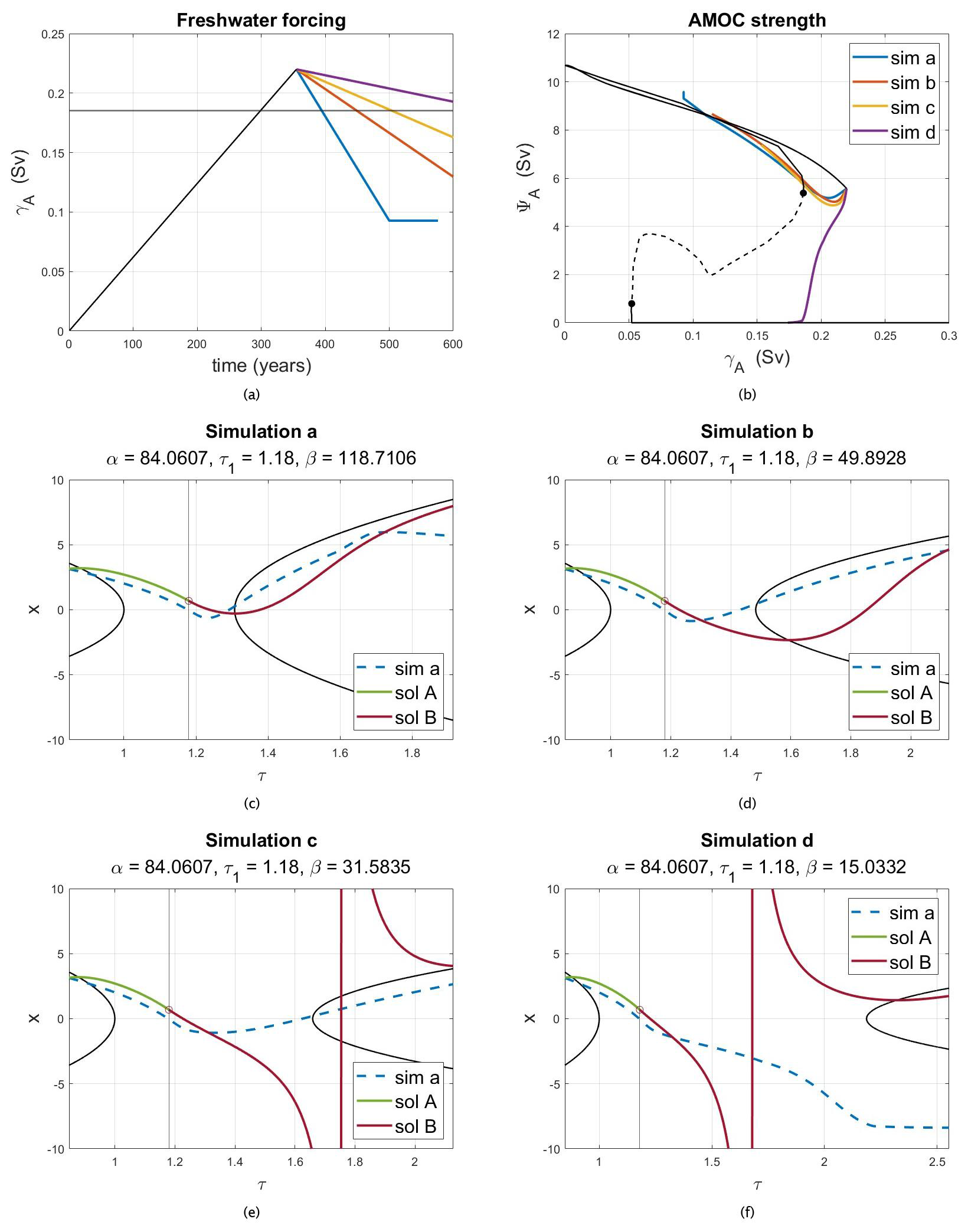
Figure 8 Global ocean model simulations considered for the comparison with the analytical solutions. (a) Forcing scenario and (b) the associated AMOC trajectories with the corresponding colors. The purple forcing has the slowest rate of decrease, and its AMOC trajectory shows a collapse; the other simulations show an AMOC recovery. (c–f) Four rescaled AMOC trajectories of the global ocean model (dashed lines) and the analytical solutions computed with the corresponding forcing parameters.

To be able to compare the simulations to the analytical solutions, we transform the simulation data Ψ_A(t) and the simulation parameters using Eq. (14). The parameters m₁,t₁ and m₂ translate respectively to α=84.061, τ₁=1.18 ($max\left(f\right)=f\left({\mathit{\tau }}_{\mathrm{1}}\right)=\mathrm{15.13}$) and $\mathit{\beta }=\mathit{\{}\mathrm{118.71},\mathrm{49.89},\mathrm{31.58},\mathrm{15.03}\mathit{\}}$.

The transformed AMOC trajectories are plotted vs. time in Fig. 8c–f (dashed curves) together with the analytical solution of the ODE in Eq. (11) computed with the same forcing parameters. The green part (sol A) corresponds to the solution in the time interval of forcing growth and the red part (sol B) to the solution in the time interval of forcing decline. Figure 8c shows that the simulation with the largest β(118.71) and hence the fastest decrease is the best-approximated simulation. The smaller β gets, the worse the approximation becomes. In Fig. 8d, for instance, the minimum of the analytical solution is larger (in absolute value) and is reached with a certain delay compared to the numerical simulation from the global ocean model. Figure 8e shows an AMOC recovery in the ocean model, whereas the corresponding analytical solution of the ODE instead exhibits a collapse. In Fig. 8f, both the numerical simulation and the analytical solution show an AMOC collapse. However, the simulation spends a longer time between the on and off state (it reaches the collapsed state at τ=2.25), while the analytical solution goes to −∞ much quicker (for ${\mathit{\tau }}^{*}=\mathrm{1.65}$).

One of the possible reasons why the approximation may not always work well is that the ODE approximates the behavior of the AMOC only locally around the saddle-node bifurcation and it is possible that the simulations performed were not close enough to the tipping point. Another reason could be the choice of Ψ_A as the main variable X. The state variable in the global ocean model is multi-dimensional, while the bifurcation diagram used for the quadratic fitting is just a one-dimensional projection. Although the strength of the AMOC does exhibit a saddle-node bifurcation, it is also part of the projection of the state variable onto the eigenvector associated with this bifurcation. Incorporating the Lyapunov–Schmidt reduction method or center manifold reduction method (Guckenheimer and Holmes, 1990) could help in addressing this issue. These methods reduce the complexity of the multi-dimensional problem by decomposing it into a simpler, lower-dimensional form while capturing the essence of the bifurcation behavior. They would allow us to identify the behavior of the global ocean model near the bifurcation point, but its application to this large-dimensional model is outside the scope of this paper.

5 Summary and discussion

We investigated the behavior of the Atlantic Meridional Overturning Circulation (AMOC) in response to overshoot scenarios under freshwater forcing. Our findings are in line with previous research that has investigated AMOC tipping behavior and the potential for recovery following temporary threshold exceedance (Ritchie et al., 2021). Slow-onset tipping elements like the AMOC may exhibit a delayed collapse, allowing for carefully managed overshoot scenarios that avoid irreversible state transitions. Our results expand on these studies by identifying the precise physical mechanisms for a safe or unsafe overshoot of the AMOC in a more detailed global ocean model.

We apply a piecewise linear freshwater forcing that grows to a maximum above the tipping point and then decreases towards a constant value. Our results confirm that overshoots can be safe under certain scenarios even if the AMOC exceeds the tipping point, contributing to the understanding of transient tipping behavior within the climate system. Similarly to Ritchie et al. (2021), our results show that the AMOC response is highly sensitive to both the rate at which the freshwater forcing increases to its peak and then decreases, as well as the initial strength of the AMOC before the forcing begins to decline. Specifically, we find that faster declines in forcing after reaching a peak are more likely to enable safe overshoot trajectories, allowing the AMOC to eventually recover. Conversely, prolonged exposure to high freshwater forcing – which mainly causes the AMOC to be weaker – significantly increases the risk of a transition to a collapsed state, which does not recover once the freshwater forcing settles to a constant value.

The key to understand the different behavior of the AMOC under different forcings is to be found in the salt fluxes of the northern North Atlantic region. When the lateral salt fluxes that transport saline water northward can counterbalance the freshwater input, making the region effectively saltier, the AMOC is able to recover; otherwise it is driven toward collapse. This delicate interplay between surface and advective salt fluxes presents a tangible metric that could serve as a reliable indicator of the AMOC trajectory towards recovery. Specifically, the time derivative of the integrated salt content in the northern region goes through zero and changes sign when the AMOC is headed toward a recovery. The North Atlantic starts to receive more saline water, reinstating a larger meridional salinity difference which directly affects the meridional density difference that drives the AMOC. Although the global ocean model has a very coarse resolution and many other major limitations (Weijer et al., 2003; Dijkstra, 2007), this mechanism is expected to be robust.

Indeed, this understanding could be useful in guiding global climate policies to mitigate and avoid the long-term consequences of an AMOC collapse (Armstrong-McKay et al., 2022). For instance, one could combine different forcing shapes, rates and peaks to explore a broader range of AMOC responses. By varying these factors, one could identify threshold conditions under which the AMOC recovers or collapses. Testing slower forcing declines in recovery scenarios or sharper declines in collapse scenarios may reveal clear transition zones that could help create a response map or define a scaling law, with forcing rates and peaks as parameters, to systematically map the AMOC responses across various scenarios. Such an approach would extend the strictly local (to the saddle-node) approach of Ritchie et al. (2019), who established an inverse-square law between time spent by the AMOC over the tipping point and amplitude of the overshoot.

In this context, the analytical approximation in Sect. 4 could serve as an initial step towards refining predictions of the AMOC responses to different forcing parameters. This framework opens the way to identify regions of safe/unsafe overshoot delimited by critical curves within the parameter space (Li et al., 2019). It could provide a clearer picture of the AMOC sensitivity to external forcing overshoot utilizing solely the bifurcation diagram from the global ocean model. However, it is crucial to acknowledge its limitations in capturing the complex dynamics of the ocean. While the approximation serves as a valuable conceptual tool, at the moment its simplicity comes at the cost of detailed accuracy. The model locality and reduced complexity do not account for any feedback mechanisms, spatial heterogeneities or other nonlinear processes that are critical in the real-world behavior of the AMOC. Future work could aim to refine this analytical framework to enhance its accuracy while still maintaining a level of simplicity that allows for broader accessibility and application in the context of AMOC studies.

To enhance our understanding of the potential for AMOC recovery in transient overshoot scenarios, future research could integrate the insights gained from our study into state-of-the-art climate models. Notably, the CESM model, for which the AMOC tipping point has been detected through quasi-equilibrium simulations (van Westen et al., 2024), provides a promising framework for such investigations. Simulating controlled freshwater forcings that mimic realistic overshoot trajectories would involve an increase in freshwater input faster than those used to identify the AMOC threshold. After having reached a forcing peak beyond the detected tipping point, the rate of freshwater decrease should be strategically adjusted to explore conditions leading to both recovery and collapse. This approach would allow detailed study of the salt transport terms in a more detailed model, offering critical insights into the processes governing AMOC stability and resilience.

The implications of our findings extend beyond theoretical interest, offering insights relevant to climate policy. The urgency to understand and minimize climate tipping risks has been recognized in international climate policy for the first time at the 27th Conference of the Parties (COP27). The Paris Agreement was aiming to limit the global temperature increase to 1.5 °C above pre-industrial levels (UNFCCC, 2015), but current climate policy scenarios are estimated to result in 2.6 °C warming above pre-industrial levels (Rogelj et al., 2023) by the end of this century (with a range of 1.7–3.0 °C). Even if the global mean temperature was to be stabilized below 1.5 °C in the long term, a temporary overshoot above 1.5 °C is a clear possibility (Bustamante et al., 2023), underlining the urgency that potential impacts and associated risks of such an overshoot need to be assessed.

Finally, the AMOC plays a vital role in regulating Northern Hemisphere climate, and a permanent AMOC collapse would likely have severe impacts on global weather patterns, potentially leading to altered precipitation and more extreme climate events (van Westen et al., 2024; Armstrong-McKay et al., 2022; Meccia et al., 2023). Our study suggests that a controlled, temporary overshoot in freshwater forcing – analogous to transient emissions scenarios – could provide policymakers with a degree of flexibility in carbon emission targets, provided the decline in forcing is managed to support AMOC recovery.

Appendix A

To compute the complete analytical solutions, it is recognized that Eq. (11) is a Riccati equation. Hence, it can be transformed (Li et al., 2019) from a first-order nonlinear ODE to a second-order linear ODE through the change in variable $x=\frac{\mathrm{1}}{u}\frac{\mathrm{d}u}{\mathrm{d}\mathit{\tau }}$. In this way it becomes

$$\begin{array}{}\text{(A1)}& {\displaystyle }{\displaystyle \frac{\mathrm{d}u}{\mathrm{d}\mathit{\tau }}}=-f\left(\mathit{\tau }\right)u=-\left\{\begin{array}{ll}-\mathit{\alpha }(\mathrm{1}-\mathit{\tau })u& {\mathit{\tau }}_{\mathrm{0}}<\mathit{\tau }<{\mathit{\tau }}_{\mathrm{1}},\\ \left(\mathit{\beta }\right(\mathrm{1}-\mathit{\tau })+k)u& \mathit{\tau }>{\mathit{\tau }}_{\mathrm{1}}.\end{array}\right.\end{array}$$

We are interested in the solutions satisfying the initial condition x(τ₀)=x₀, and, without loss of generality, we can take $\frac{\mathrm{d}u}{\mathrm{d}\mathit{\tau }}=x_{\mathrm{0}}$ and u(τ₀)=1. The solution to Eq. (A1) can then be expressed in terms of Airy functions (Ai and Bi).

$$\begin{array}{}\text{(A2)}& {\displaystyle }{\displaystyle }u\left(\mathit{\tau }\right)=\left\{\begin{array}{l}{\left[C_{\mathrm{1}}\text{Ai}\left(z\right)+C_{\mathrm{2}}\text{Bi}\left(z\right)\right]}_{z=\sqrt[\mathrm{3}]{\mathit{\alpha }}(\mathrm{1}-\mathit{\tau })}\\ {\mathit{\tau }}_{\mathrm{0}}<\mathit{\tau }<{\mathit{\tau }}_{\mathrm{1}}\\ {\left[K_{\mathrm{1}}\text{Ai}\left(w\right)+K_{\mathrm{2}}\text{Bi}\left(w\right)\right]}_{w=\sqrt[\mathrm{3}]{\mathit{\beta }}(\mathit{\tau }-\mathrm{1})-k/{\mathit{\beta }}^{\mathrm{2}/\mathrm{3}}}\\ \mathit{\tau }>{\mathit{\tau }}_{\mathrm{1}}\end{array}\right.\end{array}$$

Rescaling back in terms of x, the solution to Eq. (11) is

$$\begin{array}{}\text{(A3)}& {\displaystyle }{\displaystyle }x\left(\mathit{\tau }\right)=\left\{\begin{array}{l}-\sqrt[\mathrm{3}]{\mathit{\alpha }}{\left[\frac{C_{\mathrm{1}}\frac{\mathrm{d}\text{Ai}\left(z\right)}{\mathrm{d}z}+C_{\mathrm{2}}\frac{\mathrm{d}\text{Bi}\left(z\right)}{\mathrm{d}z}}{C_{\mathrm{1}}\text{Ai}\left(z\right)+C_{\mathrm{2}}\text{Bi}\left(z\right)}\right]}_{z=\sqrt[\mathrm{3}]{\mathit{\alpha }}(\mathrm{1}-\mathit{\tau })}\\ {\mathit{\tau }}_{\mathrm{0}}<\mathit{\tau }<{\mathit{\tau }}_{\mathrm{1}},\\ \sqrt[\mathrm{3}]{\mathit{\beta }}{\left[\frac{K_{\mathrm{1}}\frac{\mathrm{d}\text{Ai}\left(w\right)}{\mathrm{d}w}+K_{\mathrm{2}}\frac{\mathrm{d}\text{Bi}\left(w\right)}{\mathrm{d}w}}{K_{\mathrm{1}}\text{Ai}\left(w\right)+K_{\mathrm{2}}\text{Bi}\left(w\right)}\right]}_{w=\sqrt[\mathrm{3}]{\mathit{\beta }}(\mathit{\tau }-\mathrm{1})-k/{\mathit{\beta }}^{\mathrm{2}/\mathrm{3}}}\\ \mathit{\tau }>{\mathit{\tau }}_{\mathrm{1}},\end{array}\right.\end{array}$$

where the constants are

$$\begin{array}{ll}{\displaystyle }{C}_{\mathrm{1}}& {\displaystyle }={\left[{\displaystyle \frac{\frac{\mathrm{d}\text{Bi}\left(z\right)}{\mathrm{d}z}+\frac{x_{\mathrm{0}}}{\sqrt[\mathrm{3}]{\mathit{\alpha }}}\text{Bi}\left(z\right)}{\text{Ai}\left(z\right)\frac{\mathrm{d}\text{Bi}\left(z\right)}{\mathrm{d}z}-\text{Bi}\left(z\right)}}{\displaystyle \frac{\mathrm{d}\text{Ai}\left(z\right)}{\mathrm{d}z}}\right]}_{z=\sqrt[\mathrm{3}]{\mathit{\alpha }}(\mathrm{1}-{\mathit{\tau }}_{\mathrm{0}})},\\ {\displaystyle }{C}_{\mathrm{2}}& {\displaystyle }={\left[{\displaystyle \frac{-\frac{x_{\mathrm{0}}}{\sqrt[\mathrm{3}]{\mathit{\alpha }}}\text{Ai}\left(z\right)-\frac{\mathrm{d}\text{Ai}\left(z\right)}{\mathrm{d}z}}{\text{Ai}\left(z\right)\frac{\mathrm{d}\text{Bi}\left(z\right)}{\mathrm{d}z}-\text{Bi}\left(z\right)\frac{\mathrm{d}\text{Ai}\left(z\right)}{\mathrm{d}z}}}\right]}_{z=\sqrt[\mathrm{3}]{\mathit{\alpha }}(\mathrm{1}-{\mathit{\tau }}_{\mathrm{0}})},\end{array}$$

and

$$\begin{array}{ll}{\displaystyle }{K}_{\mathrm{1}}& {\displaystyle }={\left[{\displaystyle \frac{\frac{\mathrm{d}\text{Bi}\left(z\right)}{\mathrm{d}z}-\frac{x_{\mathrm{0}}}{\sqrt[\mathrm{3}]{\mathit{\beta }}}\text{Bi}\left(z\right)}{\text{Ai}\left(z\right)\frac{\mathrm{d}\text{Bi}\left(z\right)}{\mathrm{d}z}-\text{Bi}\left(z\right)}}{\displaystyle \frac{\mathrm{d}\text{Ai}\left(z\right)}{\mathrm{d}z}}\right]}_{w=\sqrt[\mathrm{3}]{\mathit{\beta }}({\mathit{\tau }}_{\mathrm{1}}-\mathrm{1})-k/{\mathit{\beta }}^{\mathrm{2}/\mathrm{3}}},\\ {\displaystyle }{K}_{\mathrm{2}}& {\displaystyle }={\left[{\displaystyle \frac{\frac{x_{\mathrm{0}}}{\sqrt[\mathrm{3}]{\mathit{\beta }}}\text{Ai}\left(z\right)-\frac{\mathrm{d}\text{Ai}\left(z\right)}{\mathrm{d}z}}{\text{Ai}\left(z\right)\frac{\mathrm{d}\text{Bi}\left(z\right)}{\mathrm{d}z}-\text{Bi}\left(z\right)\frac{\mathrm{d}\text{Ai}\left(z\right)}{\mathrm{d}z}}}\right]}_{w=\sqrt[\mathrm{3}]{\mathit{\beta }}({\mathit{\tau }}_{\mathrm{1}}-\mathrm{1})-k/{\mathit{\beta }}^{\mathrm{2}/\mathrm{3}}}.\end{array}$$