Physics of AMOC multistable regime shifts due to freshwater biases in an EMIC

The Atlantic Meridional Overturning Circulation (AMOC), an important circulation system that modulates the global climate, has been identified as a potential tipping element. To assess AMOC tipping, climate models are used that are known to have many biases, and it is unknown how these biases affect AMOC stability. We focus here on freshwater biases over the Indian and Atlantic oceans, as identified in CMIP6 models. Next, we use CLIMBER-X, an Earth system model of intermediate complexity (EMIC), to study the effect of biases in surface freshwater flux on AMOC tipping behavior. We introduce biases in the Indian and Atlantic oceans and perform hysteresis experiments where we slowly ramp up the surface freshwater forcing in the North Atlantic until the AMOC collapses; subsequently, the forcing is reversed until the AMOC recovers again. We find that negative (positive) biases in the Indian Ocean make the AMOC more unstable (stable), whereas negative (positive) biases in the Atlantic Ocean make the AMOC more stable (unstable). When biases are introduced in both the Atlantic and Indian oceans, the tipping point associated with the AMOC collapse is hardly affected. These results show that, if the freshwater bias we applied in the Indian Ocean is larger than the one applied in the Atlantic Ocean, the AMOC is more stable in CLIMBER-X. For more reliable assessments of AMOC tipping under future emission scenarios, (freshwater) bias reduction in climate models is therefore thought to be essential.

1 Introduction

The Atlantic Meridional Overturning Circulation (AMOC) has been identified as a potential tipping element due to the possible existence of multiple stable equilibria (Lenton et al., 2008; Armstrong-McKay et al., 2022). Stommel (1961) already suggested the existence of multiple stable equilibria in a simple box model. Since then, evidence of multiple stable equilibria has been found in models over the full complexity range (Rahmstorf, 1996; Rahmstorf et al., 2005; Dijkstra, 2007; van Westen and Dijkstra, 2023), along with indications in paleoclimatic proxies (Broecker et al., 1985; Lynch-Stieglitz, 2017; Weijer et al., 2019). Currently, the AMOC is in a strong, so-called “on” state, but studies suggest that it can also be in a weak or even collapsed “off” state (Weijer et al., 2019; van Westen and Dijkstra, 2023). Tipping of the AMOC would have dire consequences for the climate system, ecosystems, and society. It would lead to large-scale cooling in the Northern Hemisphere but warming in the Southern Hemisphere (Jackson et al., 2015; Liu et al., 2017; van Westen et al., 2024), a shift in precipitation patterns (Stouffer et al., 2006; Vellinga and Wood, 2008; Liu et al., 2017; Orihuela-Pinto et al., 2022; van Westen et al., 2024), and a change in wind patterns (Orihuela-Pinto et al., 2022). An AMOC weakening or collapse would also lead to local changes in sea level with potential increases in the Atlantic basin (Levermann et al., 2005; Yin et al., 2010; van Westen et al., 2024). Furthermore, the global carbon cycle (Zickfeld et al., 2008; Boot et al., 2024) and marine ecosystems (Schmittner, 2005; Boot et al., 2023, 2025) are (negatively) affected as well. Another threat is so-called tipping cascades, where tipping of the AMOC might lead to the tipping of other tipping elements, such as the Amazon rainforest and the West Antarctic Ice Sheet (Dekker et al., 2018; Sinet et al., 2023; Wunderling et al., 2024).

Measurements of the AMOC are currently too short to accurately say whether the AMOC is decreasing or not (Lobelle et al., 2020). However, there are studies that have looked at proxies of the AMOC strength. Several of these studies state that the AMOC has been declining in strength over the last 100 to 1000 years (Dima and Lohmann, 2010; Rahmstorf et al., 2015; Caesar et al., 2018, 2021), though there are also papers that find no decline in the AMOC strength. (Worthington et al., 2021; Latif et al., 2022; Rossby et al., 2022; Terhaar et al., 2025). Under climate change, the AMOC is projected to decrease in CMIP6 models, but no full collapse is found before 2100 (Weijer et al., 2020). When simulations are extended past 2100, models can show an AMOC collapse (Romanou et al., 2023). Partly based on the CMIP6 models, the IPCC AR6 report (IPCC, 2023) states that it is unlikely that the AMOC will collapse this century.

However, these models might not be suitable to make a good assessment about AMOC stability. For example, they struggle to represent past AMOC changes accurately (McCarthy and Caesar, 2023) and often do not include Greenland Ice Sheet melt. Recent studies contradict the AR6 report and suggest that the probabilities of a collapse are much higher than previously thought (Michel et al., 2022; Ditlevsen and Ditlevsen, 2023; van Westen et al., 2024). One reason for the underestimation of collapse probability in previous studies could be that biases in CMIP6 models lead to a AMOC that is too stable (Liu et al., 2017). An important metric in this regard is the freshwater transport by the AMOC over 34° S indicated here by F_ov,S, which is an indicator of the sign and strength of the salt–advection feedback (Vanderborght et al., 2025). It was earlier suggested that F_ov,S is a potential indicator whether the AMOC is in a monostable regime ($F_{\mathrm{ov},\mathrm{S}}>\mathrm{0}$) or in a multistable regime ($F_{\mathrm{ov},\mathrm{S}}<\mathrm{0}$) (Dijkstra, 2007; Weijer et al., 2019). However, recent results show that even AMOC states with $F_{\mathrm{ov},\mathrm{S}}>\mathrm{0}$ can be in a multistable regime (van Westen and Dijkstra, 2023). From observations, F_ov,S is negative (Bryden et al., 2011; Garzoli et al., 2013; Arumí-Planas et al., 2024), meaning that the salt–advection feedback is destabilizing the AMOC. In most CMIP3 (Drijfhout et al., 2011), CMIP5 (Mecking et al., 2017), and CMIP6 (van Westen and Dijkstra, 2024) models, F_ov,S is positive, which suggests that the salt–advection feedback is stabilizing the AMOC. In van Westen and Dijkstra (2024), the biases in F_ov,S were attributed to biases in the Indian Ocean which potentially make the AMOC more stable (Dijkstra and van Westen, 2024). There is, however, some criticism on using F_ov,S as a stability indicator, since not all models show a clear relation between AMOC variations and F_ov,S sign (Haines et al., 2022; Jackson et al., 2023a). Also, the effects of salinity biases in the North Atlantic and their relation to deep convection in the AMOC have been studied (Danabasoglu et al., 2014; Heuzé, 2021; Jackson and Petit, 2022; Jackson et al., 2023b), and it was found that the salinity in the Labrador Sea in particular influences important AMOC characteristics. Another important bias is the double ITCZ bias that is present in most CMIP models (Tian and Dong, 2020), and this bias has already been suggested to be a reason for an AMOC that is too stable (Liu et al., 2014).

In this study, we thoroughly investigate the effect of freshwater biases in the Indian and Atlantic oceans, representing the double ITCZ bias on AMOC stability in CLIMBER-X, an Earth system model of intermediate complexity (EMIC) (Willeit et al., 2022). We perform a large set of hysteresis experiments with model configurations where artificial positive and negative freshwater biases have been introduced to assess the effect of these biases on the multiple equilibria regime of the AMOC.

2 Methods

2.1 CLIMBER-X

CLIMBER-X consists of components simulating the atmosphere (the semi-empirical statistical–dynamical atmosphere model, SESAM), land (PALADYN), sea ice (the Simple Sea Ice Model, SISIM), and ocean (GOLDSTEIN). There are also components available within CLIMBER-X for ocean biogeochemistry (HAMOCC) and ice sheets (SICOPOLIS or Yelmo), but these are not used in this study. All submodules are run on a rectilinear 5°-by-5° latitude–longitude grid. Due to this low resolution, we can simulate almost 10 000 model years per day, allowing us to perform many experiments to systematically study the AMOC multistable regime. Below, a short description of the atmosphere, ocean, sea ice, and land models is provided, but, for a more thorough description of the model, we refer the reader to Willeit et al. (2022).

The atmosphere model in CLIMBER-X is the semi-empirical statistical–dynamical atmosphere model (SESAM). During the development of SESAM, extensive observational data were used, along with results from global climate models (GCMs). SESAM can be classified as a 2.5D model, where all prognostic variables (e.g., temperature, specific humidity, and eddy kinetic energy) are determined on a 2D grid and where the vertical dimension is purely diagnostic. The 3D structures of relative humidity and temperature are estimated using assumptions about the general vertical structure in the atmosphere of these variables, and the 3D structure of the wind is approximated using the thermal wind balance. Certain diagnostic variables, i.e., water transport, horizontal energy transport, and vertical fluxes of longwave radiation, are determined using this 3D structure. Longwave radiation fluxes take several greenhouse gases into account, i.e., CH₄, N₂O, CFCs, O₃, and CO₂, along with dust particles and sulfate aerosols. Of these, the O₃ and sulfate aerosol fields need to be prescribed to the model. Clouds are also represented in SESAM, with one cloud layer having variables such as cloud fraction, cloud top height, and cloud optical thickness.

The ocean model in CLIMBER-X is based on the GOLDSTEIN model (Edwards et al., 1998; Edwards and Shepherd, 2002; Edwards and Marsh, 2005). A major change compared to the original GOLDSTEIN model is that, for the use in CLIMBER-X, the equations are dimensionalized. GOLDSTEIN is run with 23 non-equidistant vertical layers. Horizontal velocities are determined using a frictional–geostrophic balance, the continuity equation is used to diagnose vertical velocities, and hydrostatic balance is assumed. The model uses a rigid-lid approximation, meaning that freshwater fluxes at the surface are transformed into virtual salt fluxes. For each time step, the virtual salt flux is corrected such that the globally integrated flux is equal to zero to conserve salinity. A major drawback of models based on the frictional–geostrophic balance is that the Antarctic Circumpolar Current is too weak due to momentum damping that is too strong (Edwards and Marsh, 2005; Müller et al., 2006).

The Simple Sea Ice Model (SISIM) is the sea ice model employed in CLIMBER-X. It represents one snow layer on top of one ice layer. The snow layer can accumulate and melt, and, if the layer gets deeper than 1 m, the excess becomes ice. As described above, the sea ice can accumulate due to a deep snow layer and can experience melting from above and below. The sea ice layer can also increase due to accretion from below. The freezing temperature of the seawater is dependent on the local ocean salinity through a non-linear relation. The sea ice is also allowed to drift, and the corresponding velocities are determined using an elastic–viscous–plastic rheology (Hunke and Dukowicz, 1997; Bouillon et al., 2009). SISIM also acts as a coupler between the atmosphere and ocean, including sea-ice-free regions of the ocean.

PALADYN (Willeit and Ganopolski, 2016) is the land model of CLIMBER-X and models fluxes of energy and water between the atmosphere, the land surface, and the soil. The terrestrial carbon cycle is represented and includes dynamical vegetation. In total, there are five different vegetation types: needleleaf trees, broadleaf trees, shrubs, C3-type grass, and C4-type grass. Besides these vegetation types, the land surface can be classified as bare soil, land ice, and lakes. In the soil, the temperature, water, and carbon are solved for in five vertical layers, and permafrost is explicitly represented.

2.2 Experimental setup

In all simulations presented below, we apply a freshwater forcing between 20 and 50° N in the Atlantic Ocean (see gray region in Fig. 1b) with a strength F_H. To conserve salinity, the freshwater forcing is compensated for by removing freshwater from the surface ocean globally. We first increase the freshwater forcing at a rate of 0.05 Sv kyr⁻¹ until the AMOC collapses. From a collapsed state, we linearly decrease the forcing again at the same rate until the AMOC recovers. The resulting hysteresis diagram for our baseline case, for the standard values of the parameters in CLIMBER-X, is shown in Fig. 1a. For F_H=0, the AMOC strength for this case is about 20 Sv on the forward branch (drawn curve), and, with increasing F_H, it collapses near the point S₁. The simulation of the backward branch (dashed) shows an AMOC recovery near the point S₂. Regions in freshwater forcing space smaller than S₂ are in a monostable “on” regime, and, for a freshwater forcing larger than S₁, the AMOC is in a monostable “off” regime. Between S₁ and S₂, the AMOC is in a multistable regime, as found in numerous other models (Rahmstorf, 1996; Rahmstorf et al., 2005; van Westen and Dijkstra, 2023; van Westen et al., 2025) and other studies using CLIMBER-X (Willeit et al., 2022; Willeit and Ganopolski, 2024). The existence of such a multistable regime is necessary to use this model for addressing the research questions.

There are two main reasons why the 20–50° N hosing location was chosen: (1) this region is used in many other studies using a similar experimental setup (Rahmstorf et al., 2005; Hawkins et al., 2011; van Westen and Dijkstra, 2023), and (2), by choosing this region, we do not directly affect the deep-convection sites, allowing internal feedbacks to be more dominant in the case of an AMOC collapse compared to the forcing. The hosing rate is chosen such that it is slow enough that the model does not deviate too much from its equilibrium but fast enough to still be computationally feasible.

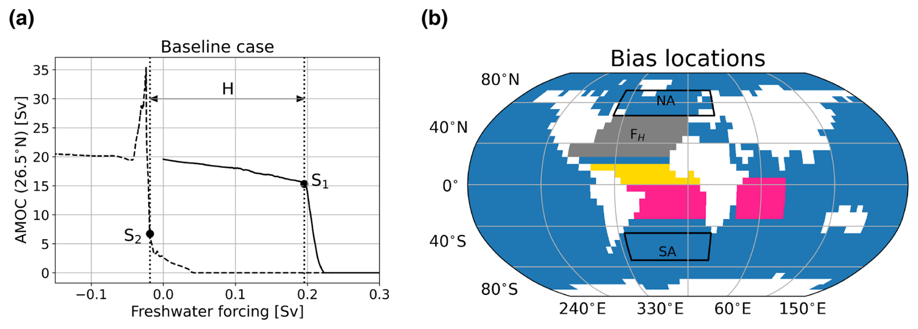
Figure 1 (a) Hysteresis diagram of the baseline case (BASE) with freshwater forcing F_H in Sv on the x axis and AMOC strength at 26.5° N in Sv on the y axis. The solid line represents the forward branch, and the dashed lines represent the backward branch. S₁ and S₂ are the collapse and recovery tipping points, and H is the hysteresis width as defined in Sect. 2.3. (b) Locations where the biases are deployed are denoted by pink and yellow. Biases in the yellow region are of opposite sign to those in the pink region and are two-thirds of the amplitude. Two boxes used for later analysis in Sect. 3.3, where variables are averaged over a North Atlantic (NA) and South Atlantic (SA) box, are also shown. The hosed region is in gray (F_H).

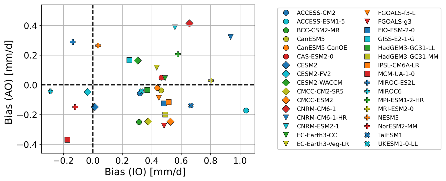
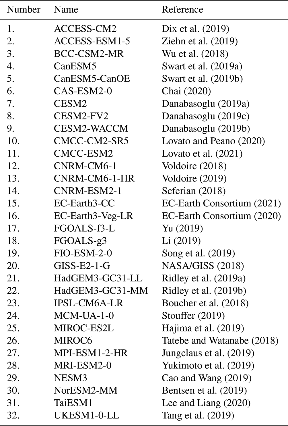
To motivate the applied biases, we consider the freshwater flux (P–E) biases in models (case BASE in CLIMBER-X and CMIP6) with respect to observations. For the latter, we take the observation-based HOAPS4.0 dataset (Andersson et al., 2017) over the period from 1994 to 2014 (21 years). The full list of 32 different CMIP6 models, from which we consider the historical simulations, is shown in Table A1. For the CMIP6 models, we use the precipitation (“pr”) and evaporation (“evspsbl”) variables to determine P–E, and, for the HOAPS dataset, we use the E–P (“EMP”) data. We average both the HOAPS dataset and model data over the pink and yellow regions indicated in Fig. 1b. Most models (27 out of 32; Fig. 2) have a positive bias in the Indian Ocean, meaning that the net effect of this bias is to freshen the Indian Ocean. Most models have a bias of approximately 0.5 mm d⁻¹ in the Indian Ocean, but the spread is quite large due to a few outliers. A total of 20 out of 32 models have a negative bias in the Atlantic Ocean. The spread for the Atlantic Ocean biases is smaller compared to the Indian Ocean biases. However, there is more variation in the exact bias strength compared to the Indian Ocean, where most models align around 0.5 mm d⁻¹.

Motivated by these CMIP6 results (Fig. 2), we add positive and negative freshwater biases in the Indian and Atlantic oceans in CLIMBER-X. Three different sets of simulations are performed where (I) biases are introduced in the Indian Ocean, (A) biases are introduced in the Atlantic Ocean, and (IA) biases are introduced in both the Indian and Atlantic oceans. Biases are introduced with six different strengths: +0.75, +1.50, and +3.00 mm yr⁻¹ for the positive biases and the negative equivalent of those for negative biases. This means that we performed 19 different simulations in total. In the Indian Ocean, the biases are introduced between 5° N to 25° S and 40 to 80° E (Fig. 1b). In the Atlantic Ocean, the biases are introduced in two sections. The southern section in the Atlantic (0° N to 25° S; pink section in Fig. 1b) receives the bias strength as mentioned above. The northern section (0 to 15° N; yellow section in Fig. 1b) receives two-thirds of the bias strength and of opposite sign to represent the double ITCZ bias found in many CMIP models (Tian and Dong, 2020). Before the hysteresis experiments are performed, a 10 000-year simulation is run to get the model in a new equilibrium after introducing the biases. In the text, we will refer to the different simulations by their bias location and bias strength. For example, I(+3.00) represents the setup with a positive bias of 3.00 mm d⁻¹ in the Indian Ocean, and IA(−0.75) represents the setup with a negative bias of 0.75 mm d⁻¹ in both the Indian and Atlantic oceans. For each of the 19 cases, we performed the same hysteresis experiment as for the baseline case, and the model is set up such that all cases have the same total salt content in the ocean at all times.

Figure 2 Biases in the Indian Ocean (x axis) versus biases in the Atlantic Ocean (y axis) in mm d⁻¹ for 32 CMIP6 models. Atlantic Ocean biases are integrated over both the pink and yellow regions in Fig. 1.

2.3 Tipping point detection

As can be seen in Fig. 1a, S₁ is the location of the tipping point representing the transition from the AMOC “on” state to the AMOC “off” state, and S₂ is the location of the tipping point representing the transition from the “off” to the “on” state (Fig. 1a). We define the hysteresis width H (in Sv) as the width in freshwater forcing F_H between the tipping points representing the transition from the “on” to the “off” state and vice versa; i.e.,

$$\begin{array}{}\text{(1)}& H={\mathrm{S}}_{\mathrm{1}}-{\mathrm{S}}_{\mathrm{2}}.\end{array}$$

We will determine the shifts of H, S₁, and S₂ in the different experiments relative to BASE, e.g., ΔH_x = H_x−H_REF, where x represents an experiment with a freshwater forcing bias.

To determine the precise location of the tipping points S₁ and S₂, we employ a method based on detecting change points using the pruned exact linear time (PELT) method (Killick et al., 2012). In this method, we are able to set the minimum time between two change points, which allows us to tune this method to some extent. In our time series, as the AMOC is collapsing or recovering, the time between change points decreases and converges towards the chosen minimum time. The minimum time between two change points for an AMOC collapse is set to 20 years, and the minimum time for an AMOC recovery is set to 5 years. We define a threshold for time between change points, i.e., 120 years for an AMOC collapse and 20 years for an AMOC recovery. Note that these threshold values are used for tuning of the method. When the time between change points becomes lower than such a threshold (t_th), we define the location of the tipping point as

$$\begin{array}{}\text{(2)}& s=X\left(t_{\mathrm{th}}\right)-\mathrm{0.5}\mathrm{\Delta }X,\end{array}$$

where s is the tipping point in time space, X is the time of the change point at t_th, and ΔX is the time between the change point at t_th and the next change point. Note that this method is subject to some subjectivity through the tuning. Hence, all tipping points are also checked visually to see whether the methodology gives reasonable results. For the IA(+3.00) simulation, this method fails and the tipping points are determined visually.

3 Results

3.1 AMOC–F_ov,S relation

The applied biases change the AMOC and F_ov,S of the equilibrium states for F_H=0. An overview of the equilibrium AMOC strength at 26.5° N and F_ov,S of the different cases is presented in Fig. 3. Case BASE is within observational bounds of F_ov,S but simulates an AMOC that is slightly too strong compared to observations. Negative biases in the Indian Ocean (cyan markers) decrease the AMOC strength and lead to a more negative F_ov,S, while positive biases (blue markers) lead to a stronger AMOC with a more positive F_ov,S. Biases in the Atlantic Ocean have an opposite effect. Negative biases (orange markers) increase the AMOC strength and lead to larger F_ov,S, and positive biases (red markers) lead to a weaker AMOC and more negative F_ov,S. A(+3.00) shows a break in the trend, since F_ov,S is larger than in A(+1.50). For the combined biases, a clear non-linear relation is seen. Negative biases (olive markers) show a stronger AMOC and more positive F_ov,S for stronger biases, whereas positive biases (green markers) show a weaker AMOC and more positive F_ov,S for stronger biases. This relation is caused by the competing effects of the biases in the Indian Ocean and Atlantic Ocean on the AMOC strength and F_ov,S.

We can explain this behavior in F_ov,S as follows: for the Indian Ocean, if a positive bias is applied, the Indian Ocean becomes more fresh, and this is transported towards the Atlantic section of the Southern Ocean. From here, less saline water is advected into the Atlantic basin across 35° S, effectively increasing the freshwater transport and therefore F_ov,S. The AMOC strengthens for positive biases because the density in the South Atlantic decreases due to freshening, which increases the meridional density difference between the North and South Atlantic. When positive biases are applied in the Atlantic Ocean, the Atlantic basin becomes fresher, which reduces the AMOC strength and consequently also the freshwater transported by the overturning circulation.

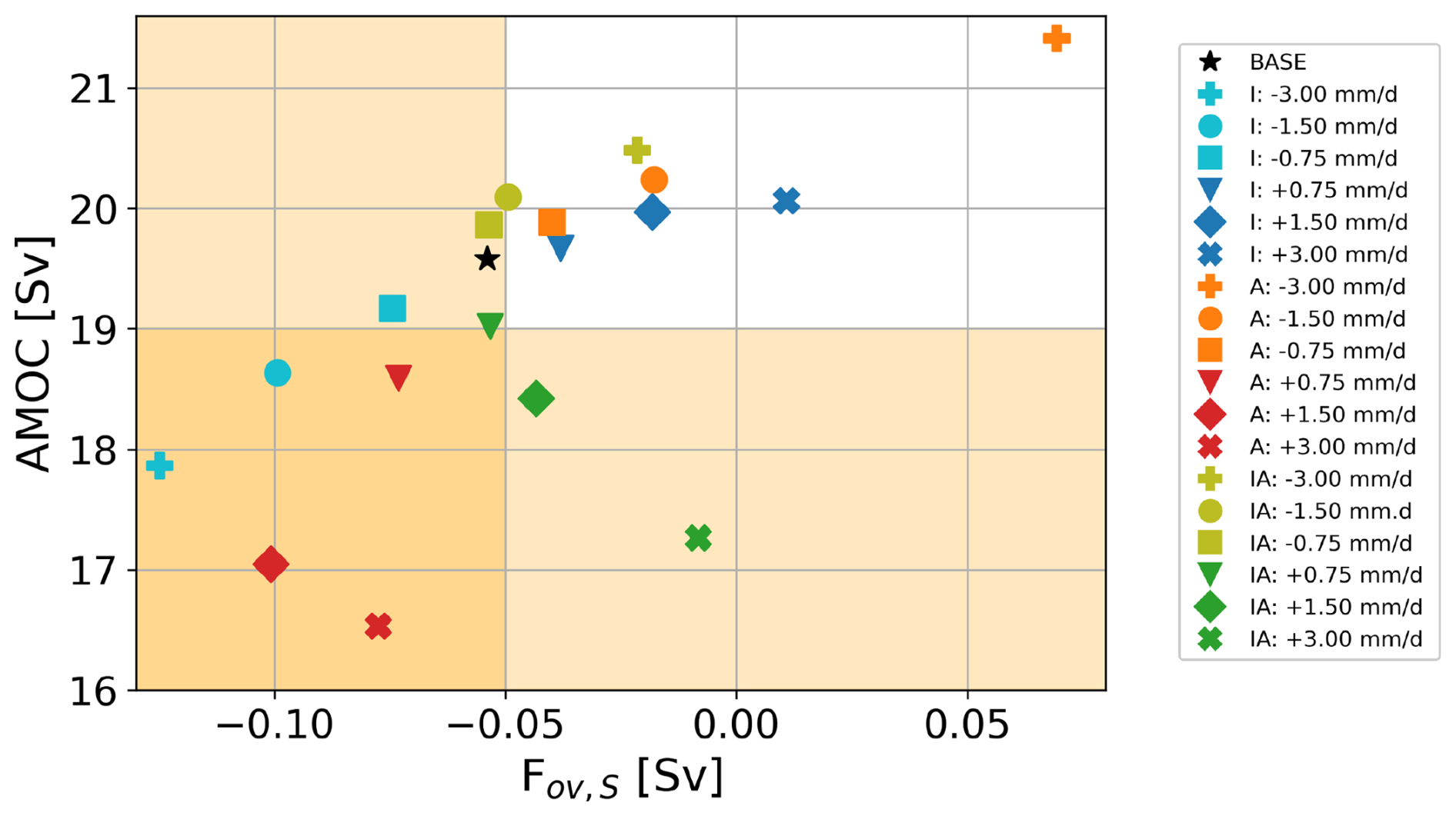
Figure 3 AMOC–F_ov,S relation in equilibrium for the different simulations with the AMOC strength at 26.5° N in Sv on the y axis and F_ov,S in Sv on the x axis. Yellow shading in the background represents observational bounds for the AMOC strength (Smeed et al., 2018; Worthington et al., 2021) and F_ov,S (Garzoli et al., 2013; Mecking et al., 2017; Arumí-Planas et al., 2024); due to the grid in CLIMBER-X, F_ov,S is determined at 35° S.

3.2 AMOC multistable regime

From Fig. 1a, we see that, for case BASE, the AMOC tips at a freshwater forcing of 0.1956 Sv (S₁) and recovers at a freshwater forcing of −0.0187 Sv (S₂), resulting in a hysteresis width H=0.2142 Sv. CLIMBER-X simulates a full AMOC collapse with no overturning in the North Atlantic in the “off” state (Fig. A1).

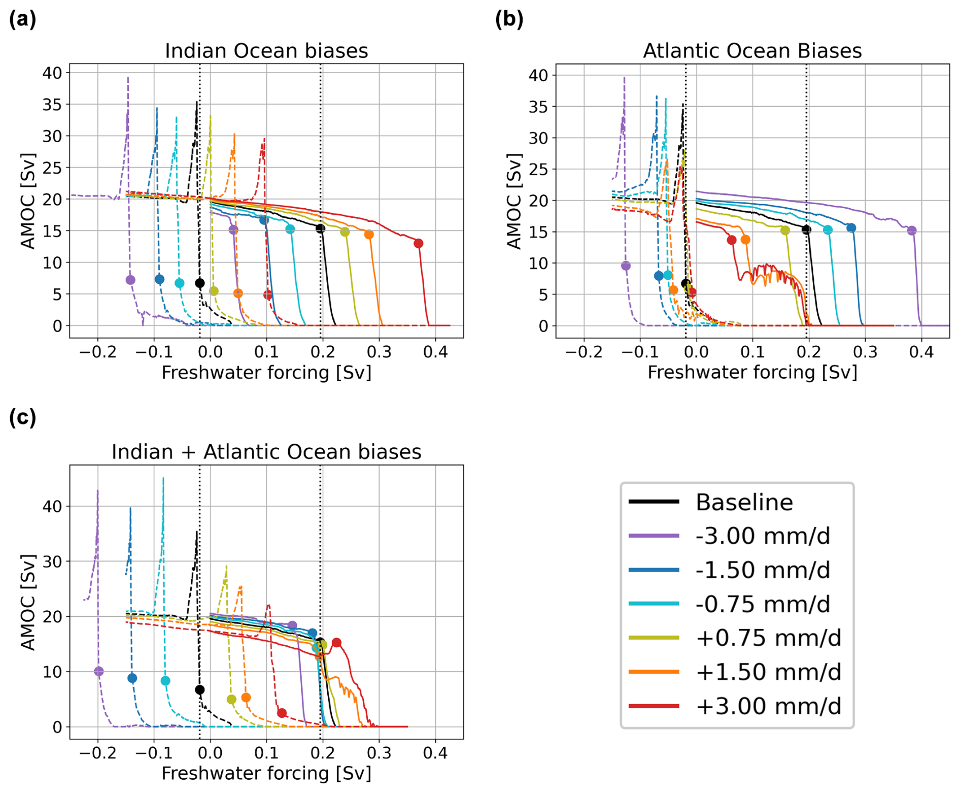
Figure 4 Hysteresis diagrams for the different simulations with AMOC strength at 26.5° N in Sv on the y axis and the strength of the freshwater forcing in Sv on the x axis. The black line represents the baseline case. Solid lines represent the forward simulation, i.e., under increasing forcing, and dashed lines represent the backward simulation under decreasing forcing. Markers represent the location of the tipping points determined by the method described in Sect. 2.3. The vertical dotted black lines represent the location of the tipping points in BASE. (a) Results for the Indian Ocean biases. (b) Results for the Atlantic Ocean biases. (c) Results for the Indian and Atlantic ocean biases.

For the cases with biases in the Indian Ocean, the hysteresis diagram shows a shift with respect to case BASE (Fig. 4a). Positive biases (i.e., an Indian Ocean that is too fresh) cause the hysteresis diagram, i.e., both S₁ and S₂, to shift towards larger freshwater forcing, whereas, for negative biases, the hysteresis diagram shifts towards smaller forcing. The biases in the Atlantic Ocean mainly cause a shift in S₁, where negative biases cause a shift towards larger forcing and positive biases cause a shift towards smaller forcing. S₂ does not shift by a lot in most experiments, except for A(−3.00). This means that the hysteresis width increases (decreases) under negative (positive) biases. Both A(+1.50) and A(+3.00) show a two-step tipping. At the markers of the tipping points (around 0.08 Sv), deep convection in the subpolar gyre collapses. This represents a weak AMOC state as found earlier in CLIMBER-X (Willeit and Ganapolski, 2024). The AMOC weakens to about 8 Sv and shows relatively strong internal variability. Around a freshwater forcing of 0.2 Sv, the AMOC fully collapses, since, at this point, deep-water formation in the Greenland–Iceland–Norwegian (GIN) seas ceases, implying that deep-water formation in the GIN seas is vital in CLIMBER-X to sustain an AMOC. For the combined biases (IA), there is mostly a shift in S₂, whereas there is hardly a shift in S₁ (Fig. 4c). Negative (positive) biases cause an increase (decrease) in the multistable regime by moving S₂ towards more negative (positive) values. Just like A(+1.50) and A(+3.00), IA(+1.50) shows a two-step tipping.

The change in location of the tipping points and the change in the hysteresis width are summarized in Fig. 5. For the Indian Ocean biases, ΔH is close to 0, with small negative values for negative biases and small positive values for positive biases. For the Atlantic Ocean biases, we can see that most markers fall along the S₂=0 contour line. However, for larger negative biases (orange markers), the deviation from this line increases. For the simulations with biases in both basins, we see that the green and olive markers are close to the line S₁=0. There is a small negative shift for negative biases and a small positive shift for positive biases. This means that, with respect to the collapse tipping points, the Indian and Atlantic ocean biases compensate each other about linearly.

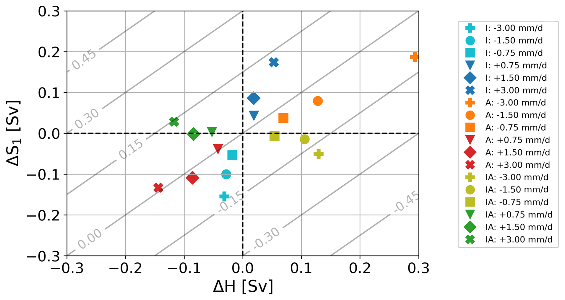
Figure 5 Overview of the change in hysteresis width (ΔH) and change in location of the collapse tipping point (Δ S₁) in freshwater forcing space in Sv. Dashed black lines represent ΔH=0 (vertical) or Δ S₁=0 (horizontal). Contour lines in the background represent the shift in the recovery tipping point (Δ S₂) in Sv.

3.3 Analysis

To explain the behavior seen in Sect. 3.2, we will look at surface properties in a North Atlantic box (50–70° N, 70° W–25° E) and a South Atlantic box (35–55° S, 55° W–20° E). We do this because these are the regions where we have isopycnal outcropping relevant for the AMOC strength (Wolfe and Cessi, 2015) and because, in CLIMBER-X, the AMOC is strongly related to the meridional density gradient over the Atlantic (Fig. 6). Specifically, we look at sea surface temperature (SST), sea surface salinity (SSS), and surface density for the equilibrium states at F_H=0 (Fig. 7). Additional results, showing these variables along the hysteresis diagrams, can be found in Figs. A2 to A4.

Negative biases in the Indian Ocean make the Indian Ocean more saline. This increase in salinity is transported towards the South Atlantic (cyan markers Fig. 7b). Here, it increases the density, which decreases the meridional density gradient between the North Atlantic and South Atlantic (Fig. A3g). Due to this decrease, the AMOC weakens, which reduces the transport of heat and salt towards the North Atlantic, causing cooling and freshening (cyan markers Fig. 7a). For the density, the freshening signal is dominant, meaning that density decreases in the North Atlantic (cyan markers Fig. 7a). Because of the lower surface density, a smaller value of F_H is required to block the isopycnals from outcropping in this region. This explains the shift in S₁ towards smaller values of F_H (Fig. 4a). For positive biases, the Indian Ocean freshens, which results in the opposite response to the one described above (blue markers Fig. 7).

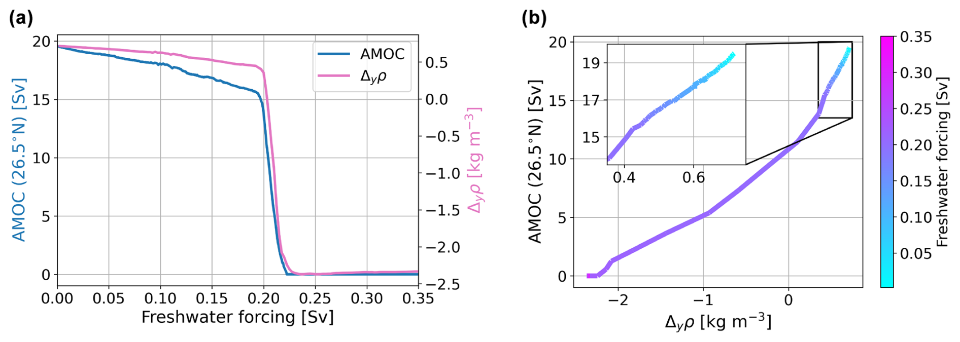
Figure 6 (a) AMOC strength at 26.5° N in Sv (blue; left y axis) and the meridional density difference Δ_yρ in kg m⁻³ (pink; right y axis) versus freshwater forcing F_H in Sv (x axis) for case BASE. (b) AMOC–Δ_yρ relation. The inset is a zoom-in before the AMOC collapse.

Negative biases in the Atlantic Ocean make the Atlantic basin more saline, including an increase in salinity in the North Atlantic (orange markers Fig. 7a). This increases the meridional density gradient (Fig. A3h), leading to a stronger AMOC, which increases SSTs and SSSs in the North Atlantic due to increased transport of heat and salt (orange markers Fig. 7a). Also, here, the salinity response is dominant for the density, meaning the surface density increases. Because of the higher surface density, more freshwater forcing is necessary to block the isopycnals from outcropping, which explains why S₁ shifts towards larger values of freshwater forcing (Fig. 4b). For positive biases, freshening of the Atlantic basin causes the opposite response to the one described above (red markers Fig. 7).

The situation is more complicated when biases are introduced in both basins. Negative biases in the Atlantic Ocean cause an increase in salinity and density in the North Atlantic, increasing the AMOC strength. Since the AMOC is exporting freshwater out of the Atlantic Ocean ($F_{\mathrm{ov},\mathrm{S}}<\mathrm{0}$), the increased AMOC causes a decrease in salinity in the South Atlantic. This effect dominates over the effects of a more saline Indian Ocean. What makes these simulations different is that the surface density in the North Atlantic is relatively independent of the strength and sign of the biases (except for the IA(+3.00) experiment), which can be seen in Fig. 7, as the olive and green markers are located on the same isopycnal as BASE (black marker). This means that the changes in salinity and temperature caused by a different AMOC strength compensate each other for the surface density in the IA experiments. Since the surface density is similar, the amount of freshwater forcing necessary to block the isopycnals from outcropping is also similar, explaining why S₁ hardly moves in the IA experiments (Fig. 4c).

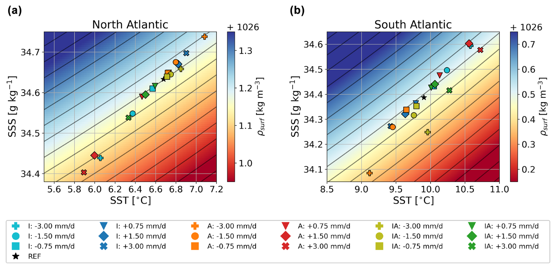
Figure 7 Sea surface temperature in °C (x axis) versus sea surface salinity in g kg⁻¹ (y axis). Coloring in the background represents surface density in kg m⁻³, and the contour lines are isopycnals. The data points represent the variables at the start of the hysteresis experiments at a freshwater forcing of 0 Sv. (a) For the North Atlantic box. (b) For the South Atlantic box.

4 Summary and discussion

This study complements previous research (Jackson et al., 2023b) in showing the importance of freshwater biases for the AMOC. Specifically, we have looked at the effect of freshwater biases, as identified in CMIP6 models, on AMOC hysteresis behavior in CLIMBER-X. We find that biases in the Indian and Atlantic oceans can shift the collapse tipping point in hysteresis experiments. Positive biases in the Indian Ocean (i.e., freshening) lead to a shift in the tipping point towards larger freshwater forcing. Positive biases in the Atlantic Ocean have an opposite effect; i.e., the tipping point shifts towards smaller freshwater forcing. When biases are introduced in both basins, the collapse tipping point does not show a shift.

In this study, we have focused on buoyancy forcing in the North Atlantic to collapse the AMOC. However, Southern Ocean processes, such as eddies and upwelling, play an important role in shaping and driving the Global Overturning Circulation and the AMOC (Kuhlbrodt et al., 2007). In higher-resolution models, these Southern Ocean processes can prevent the AMOC from fully collapsing by sustaining a very weak and shallow AMOC. In Baker et al. (2025), they suggest that the AMOC can only fully collapse if the Southern Ocean upwelling is compensated for by an emerging Pacific Meridional Overturning Circulation (PMOC), which was not the case in the CMIP6 models they analyzed. In our study, however, the upwelling is compensated for by changes in the Southern Ocean overturning circulation and a strong PMOC, allowing the AMOC to fully collapse. In a strongly eddying ocean-only model, using a similar simulation protocol as used in this study, van Westen et al. (2025) find that the AMOC does not fully collapse, which might be attributed to eddies in the Southern Ocean. However, the differences in climate impact between a fully collapsed AMOC and a very weak AMOC are small.

The width of the hysteresis of the baseline case (BASE) compares well to other models (Rahmstorf et al., 2005) and previous studies with CLIMBER-X (Willeit et al., 2022; Willeit and Ganopolski, 2024). The exact hysteresis width is dependent on (among others) the hosing rate. The rate chosen in this study is the same as in Rahmstorf et al. (2005). In Willeit and Ganopolski (2024), a slower hosing rate is also used, which results in a narrower hysteresis width with the collapse tipping point at lower freshwater forcing and the recovery tipping point at higher freshwater forcing. Notably, this shift means that the AMOC is in a monostable “on” state at F_H=0 in this model for the baseline case. However, we do not expect that a slower hosing rate would lead to different conclusions for our study, as a similar shift due to a specific bias would occur.

Although such biases have been found in CMIP6 models, it is unfortunately not yet possible to make any convincing statements on how these biases would affect AMOC stability in these models. One reason is that the background states of the CMIP6 models and the background state of CLIMBER-X are very different; hence the effects of biases are also expected to be different. Another source of uncertainty is the fact that the CLIMBER-X simulations were performed in a stable pre-industrial climate state, whereas the biases determined in the CMIP6 models are from short, transient simulations under historical forcing. There is no way to circumvent this, since we only have observations in the historical period and the hysteresis experiments need to be done in quasi-equilibrium. How this influences the conclusions of this study, we cannot say. The biases are also determined over a relatively short period. This means that if (strong) multidecadal variability is present in the freshwater fluxes, the assessed bias strength in the CMIP6 models is not a good representation of the actual model biases. Finally, besides freshwater biases, there are also biases in sea ice and surface air temperatures that may influence AMOC stability and are not considered in this study.

Because of the coarse resolution and the simple atmospheric model in CLIMBER-X, atmospheric feedbacks might not be as important in our simulations compared to CMIP6 models. The importance of changes in atmospheric heat and moisture transport in hysteresis simulations has already been shown, for example, in Jackson et al. (2016) in a different EMIC with a higher ocean resolution than CLIMBER-X. As mentioned earlier, Southern Ocean upwelling is important for shaping the AMOC as well, and CMIP6 models show a change in the Southern Ocean westerlies following an AMOC weakening, which changes the Ekman dynamics (Madan et al., 2023; Baker et al., 2025). A weakening AMOC might also decrease the wind stress curl over the North Atlantic subpolar gyre (Madan et al., 2023), which could act as positive feedback during an AMOC collapse by decreasing deep convection. These atmospheric feedbacks can play a different role in the CMIP6 models compared to CLIMBER-X and can therefore lead to a different response to freshwater biases in CMIP6 models compared to CLIMBER-X.

On the positive side, we presented a clear physical mechanism in Sect. 3.3, with an important role of the salt–advection feedback, on how the biases change the AMOC hysteresis properties in CLIMBER-X. These physical processes are also expected to be present in the CMIP6-type models. However, in CMIP6 models, other processes, e.g., the atmospheric feedbacks mentioned earlier, may become more important. To assess how important these other feedbacks are, hysteresis experiments with CMIP6-type models following a similar protocol to that in this study should be performed. Although this is computationally challenging, we hope that this paper will stimulate simulations where the effects of biases are systematically addressed in these models.

Appendix A

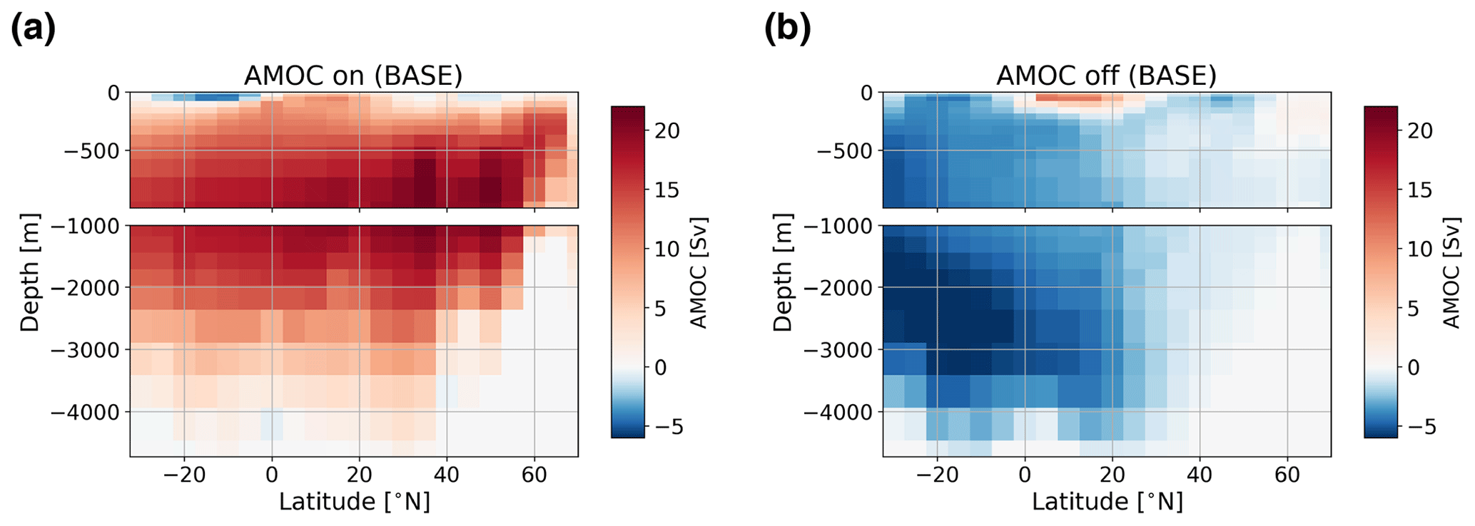
Figure A1 The AMOC in Sv in latitude (x axis)–depth (y axis) space for case BASE in (a) an “on” state at a freshwater forcing of 0 Sv and in (b) an “off” state at a freshwater forcing of 0.35 Sv.

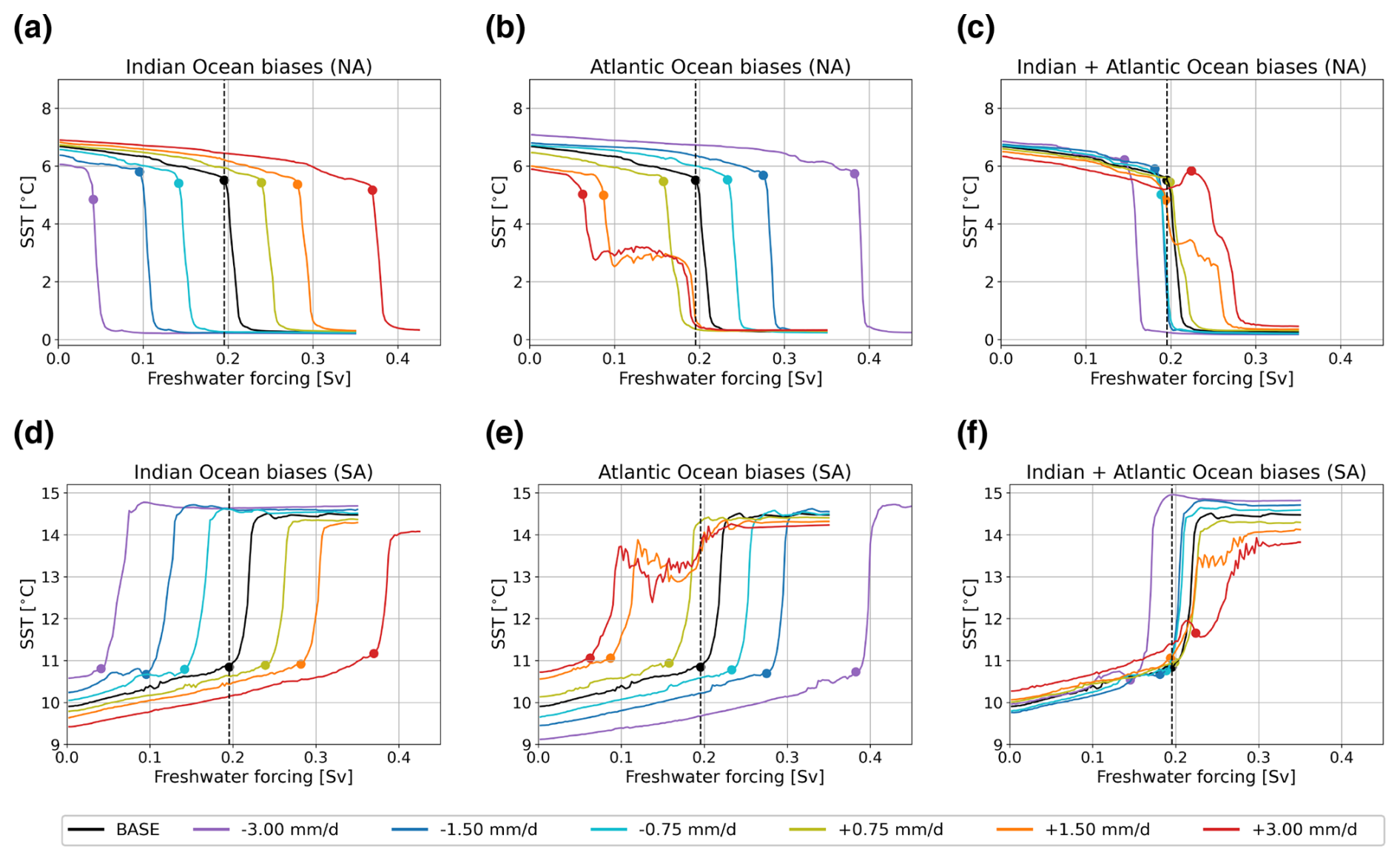
Figure A2 Sea surface temperature (SST) in °C in the North Atlantic (50–70° N, 70° W–25° E; a–c) and in the South Atlantic (35–55° S, 55° W–20° E; d–f). (a, d) For simulations with biases in the Indian Ocean. (b, e) For simulations with biases in the Atlantic Ocean. (c, f) For simulations with biases in both basins. The markers represent the tipping points, and the dashed black line represents the tipping point of BASE.

Figure A3 Same as Fig. A2 but for sea surface salinity in g kg⁻¹.

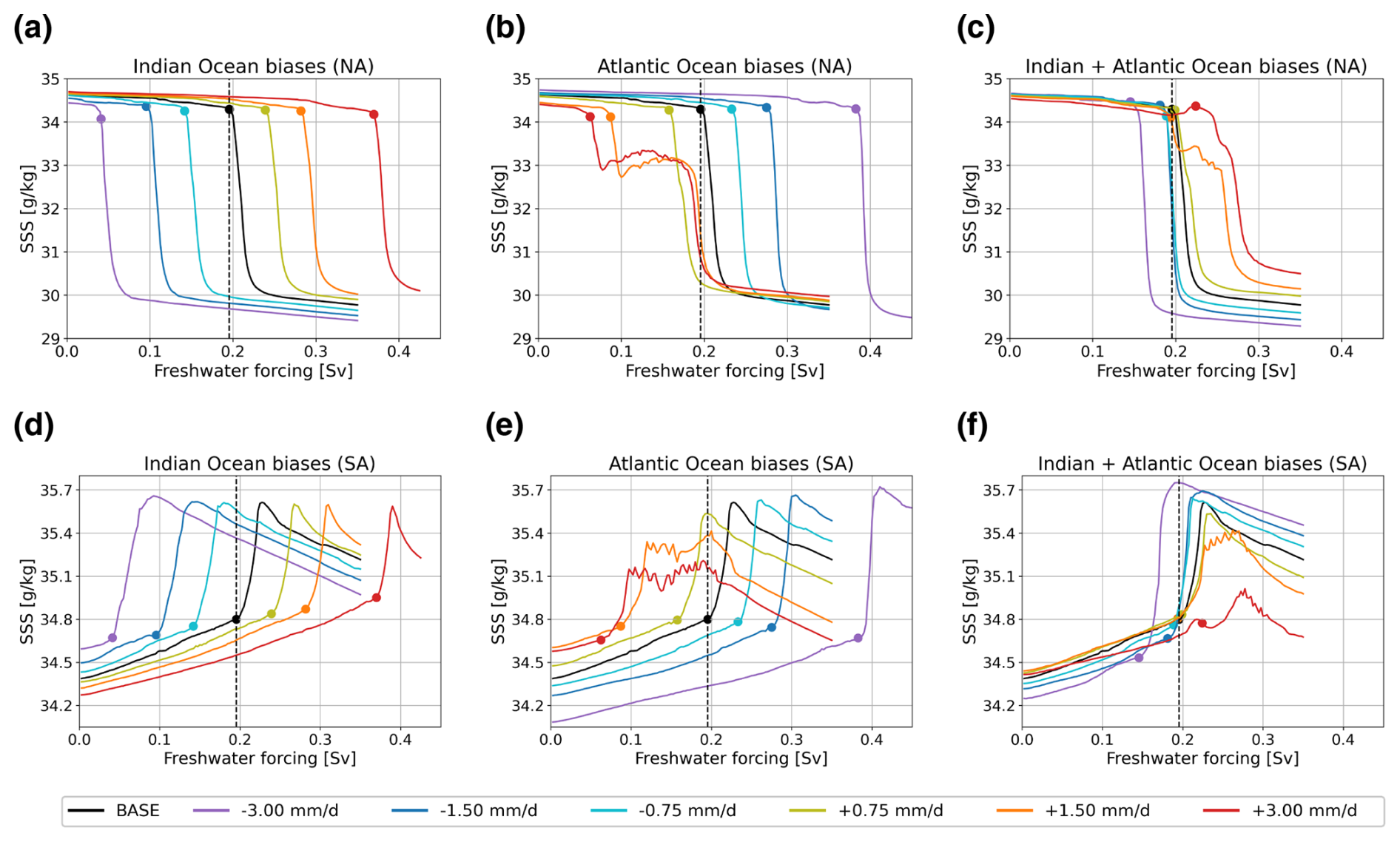
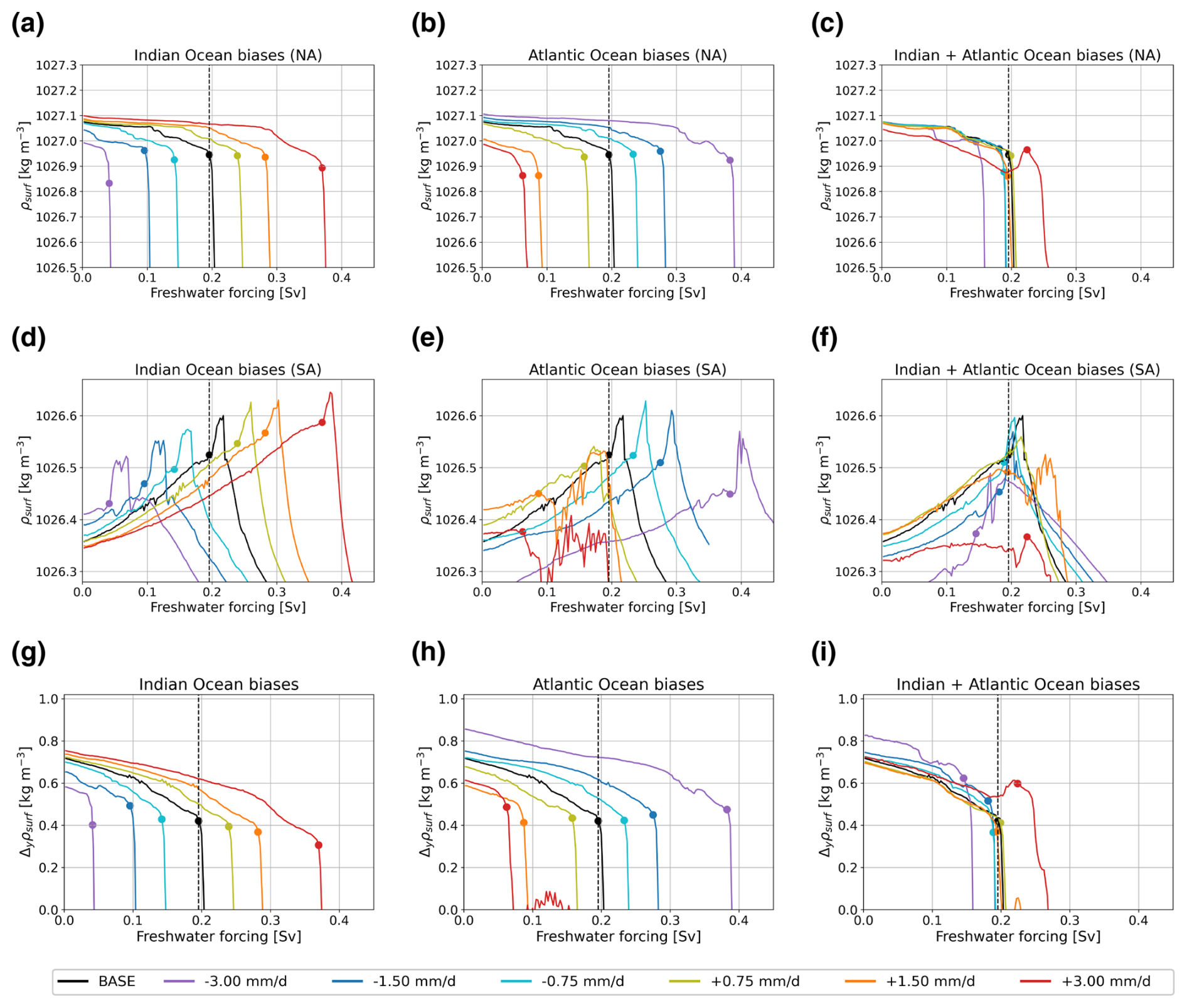
Figure A4 (a–f) As in Fig. A2 but for surface density in kg m⁻³. Panels (g–i) represent the density difference between the northern box and the southern box (ρ_N−ρ_S) in kg m⁻³ for the Indian Ocean biases (g), the Atlantic Ocean biases (h), and the biases in both basins (i).

Dix et al. (2019)Ziehn et al. (2019)Wu et al. (2018)Swart et al. (2019a)Swart et al. (2019b)Chai (2020)Danabasoglu (2019a)Danabasoglu (2019c)Danabasoglu (2019b)Lovato and Peano (2020)Lovato et al. (2021)Voldoire (2018)Voldoire (2019)Seferian (2018)EC-Earth Consortium (2021)EC-Earth Consortium (2020)Yu (2019)Li (2019)Song et al. (2019)NASA/GISS (2018)Ridley et al. (2019a)Ridley et al. (2019b)Boucher et al. (2018)Stouffer (2019)Hajima et al. (2019)Tatebe and Watanabe (2018)Jungclaus et al. (2019)Yukimoto et al. (2019)Cao and Wang (2019)Bentsen et al. (2019)Lee and Liang (2020)Tang et al. (2019)

Table A1 CMIP6 model list.