Variability and predictability of a reduced-order land–atmosphere coupled model

This study delves into the predictability of atmospheric blocking, zonal, and transition patterns utilizing a simplified coupled model. This model, implemented in Python, emulates midlatitude atmospheric dynamics with a two-layer quasi-geostrophic channel atmosphere on a β plane, encompassing simplified land effects. Initially, we comprehensively scrutinize the model's responses to environmental parameters like solar radiation, surface friction, and atmosphere–ground heat exchange. Our findings confirm that the model faithfully replicates real-world Earth-like flow regimes, establishing a robust foundation for further analysis. Subsequently, employing Gaussian mixture clustering, we successfully delineate distinct blocking, zonal, and transition flow regimes, unveiling their dependencies on surface friction. To gauge predictability and persistence, we compute the averaged local Lyapunov exponents for each regime. Our investigation uncovers the presence of zonal, blocking, and transition regimes, particularly under conditions of reduced surface friction. As surface friction increases further, the system transitions to a state characterized by two blocking regimes and a transition regime. Intriguingly, periodic behavior emerges under specific surface friction values, returning to patterns observed under low friction coefficients. A model resolution increase impacts the system in such a way that only two regimes are then obtained with the clustering: the transition phase disappears and the predictability drops to roughly 2 d for both of the remaining regimes. In accordance with previous research findings, our study underscores the fact that when all three regimes coexist, zonal patterns exhibit a more extended predictability horizon compared to blocking patterns. Remarkably, transition patterns exhibit reduced predictability when coexisting with the other regimes. In addition, within a specified range of surface friction values where two blocking regimes are found, it is observed that blocked atmospheric situations in the west of the applied topography are marked by instabilities and reduced predictability in contrast to the blockings appearing on the eastern side of the topography.

1 Introduction and motivation

Low-frequency variability (LFV) encompasses a wide range of atmospheric and climate processes, including atmospheric blockings, heat waves, cold spells, and long-term oscillations like the Madden–Julian oscillation (MJO), the North Atlantic Oscillation (NAO), and the El Niño–Southern Oscillation (ENSO). Despite extensive research, a comprehensive understanding of the nature of these LFVs remains elusive. In practical terms, exploiting these LFVs to achieve accurate extended-range forecasts beyond 2 weeks at midlatitudes remains a formidable challenge. On the climate front, comprehending how climate change affects the low-frequency variability of the atmosphere also remains an area of incomplete knowledge. Previous works, as reported in Ghil and Robertson (2002) and Lucarini and Gritsun (2020), have highlighted this gap in understanding.

Blocking systems – a notable form of LFV observed in the atmosphere – can be described as long-lasting, quasi-stationary flow patterns in the troposphere (Liu, 1994). These patterns are characterized by a significant meridional flow component, leading to a disruption or deceleration of the zonal westerly flow at midlatitudes (Nakamura and Huang, 2018). While the blocking systems persist, strong zonal flows may simultaneously exist to the north and south of them. The evolution of blocking systems involves transitions between more zonal and more meridional flow patterns during their onset and decay phases, posing challenges for forecast models (Frederiksen et al., 2004). Moreover, the dynamics of blocking systems are complex, involving interactions across different spatial and temporal scales, both internally within the system and with the surrounding flow environment (Shutts, 1983; Lupo and Smith, 1995). Researchers have highlighted the intricate nature of these dynamics and the connections between various scales, contributing to the challenges in understanding and predicting the behavior of blocking systems. As blocking systems have the potential to induce weather extreme like heat waves, there is a notable interest in understanding how the characteristics of these blocking events might evolve in the future and how such changes could subsequently impact the occurrence and features of surface extreme weather events. The investigation of these potential changes is of significant importance to assess the risks associated with extreme weather events and to enhance our understanding of the complex interactions between blocking patterns and surface weather conditions in a changing climate context (Kautz et al., 2022).

Even though the concerns above matter, identifying and evaluating LFVs in GCMs (general circulation models) constitute an computationally expensive process, so in this study an idealized reduced-order coupled model is used. It is a climate model “stripped to the bone”, which links theoretical understanding to the complexity of more realistic models, made by key ingredients and approximations; this hence helps us to study a particular phenomenon by tweaking the parameters affecting them with less computational cost. The pursuit of simplified models for atmospheric phenomena has a long history, dating back to Lorenz's seminal work in the early 1960s (Lorenz, 1960, 1962, 1963a, b). This approach recognizes the value of sacrificing some detail in exchange for a deeper grasp of fundamental physical processes.

Lorenz demonstrated the power of this strategy by leveraging Fourier series to distill the barotropic vorticity equation into three ordinary differential equations (Lorenz, 1960). These equations, while omitting smaller scales of motion, yielded valuable insights into atmospheric scenarios such as flow interactions and current stability. Subsequently, he developed a simplified geostrophic model using truncated Fourier–Bessel series (Lorenz, 1962). This eight-equation model captured baroclinic instability, a critical process in atmospheric dynamics, while maintaining key energy relationships. Notably, the model successfully reproduced observed flow regimes and transitions in rotating fluids, suggesting its effectiveness in studying large-scale atmospheric behavior. Lorenz's 1963 research yielded significant advancements in our understanding of atmospheric dynamics through two key publications (Lorenz, 1963a). The first introduced a now-iconic system of three differential equations, derived from a further simplified model for fluid flow. This ground-breaking work unveiled the concept of sensitive dependence on initial conditions, a cornerstone of chaos theory.

In the same year, Lorenz explored a separate avenue by investigating a simplified model for symmetrically heated rotating viscous fluids (Lorenz, 1963b). This work resulted in a system of 14 ordinary differential equations governed by two external parameters: the thermal Rossby number and the Taylor number. Analytical solutions revealed the existence of purely zonal flow and superimposed steady waves, while numerical integration unveiled a richer tapestry of flow behaviors. Oscillatory solutions with periodic shape changes and irregular non-periodic flow emerged. Interestingly, increasing the Taylor number generally led to greater flow complexity, except at very high values where the model's truncations became unrealistic.

Perhaps most intriguing was the coexistence of unstable, purely zonal, steady-wave, and oscillatory solutions. This suggests intricate flow dynamics, with transitions between symmetric and nonsymmetric vacillation occurring independently of instability. These findings highlight the ability of simplified models to unveil complex and nuanced behaviors in atmospheric dynamics (Shen et al., 2023). Lorenz's pioneering work in the early 1960s demonstrated the power of simplified models for understanding atmospheric dynamics. By strategically neglecting certain complexities, he was able to capture key phenomena like baroclinic instability and chaos. However, for large-scale atmospheric simulations, computational efficiency becomes paramount. This is where qg (quasi-geostrophic) models come in. Qg models prioritize large-scale features by making specific approximations, allowing for rapid simulations and analyses of broad atmospheric circulation patterns. While they may not capture the intricate details explored by Lorenz's models, qg models remain a workhorse for studying large-scale atmospheric phenomena. Hence the trend continued with Charney and DeVore (1979) in which a quasi-geostrophic model, projected onto Fourier modes for a more efficient and concise representation, was developed. It also incorporates an idealized parameterization closure to account for subgrid-scale processes. By imposing in addition a meridional temperature gradient over a topography, the model becomes a forced dissipative system, which exhibits multiple stable equilibria, representing distinct atmospheric flow patterns. Charney and Devore hypothesized that the transitions between these solutions were primarily influenced by small-scale perturbations or the presence of baroclinic instability within the system.

Charney and Straus (1980) partially confirmed this hypothesis and found that these transitions were indeed the result of baroclinic instability. Their study sheds light on the complex interactions between atmospheric flow, orography, and propagating planetary waves in baroclinic systems. They discovered that the interactions between atmospheric flow and orography induces form-drag instability, generating eddies and perturbations and leading to multiple stable equilibria with distinct flow patterns under consistent forcing conditions.

Charney's seminal study sparked significant interest in the low-order spectral model and the theory of multiple flow equilibria. Zhengxin and Baozhen (1982) and Zhu (1985) employed a two-layer low-order spectral model, discovering stable equilibrium states resembling actual blocking, with zonally asymmetric thermal and topographic forcings and flow nonlinearity playing critical roles in blocking dynamics. The summarized version of the evolution of numerical weather prediction and predictability tools is included in Yoden (1983a), Yoden (1983b), and Yoden (2007).

Reinhold and Pierrehumbert (1982) and Reinhold and Pierrehumbert (1985) extended Charney's model, incorporating additional synoptic-scale waves, revealing two distinct weather regime states influenced by wave–wave interactions causing transitions between equilibrium states.

Cehelsky and Tung (1987) demonstrated that the behavior of a reduced-order model exhibits notable disparities at higher resolutions, primarily attributed to the inadequate representation of energy upscaling and vorticity downscaling pathways. They coined this phenomenon “spurious chaos”, denoting the emergence of irregular dynamics that are not genuinely representative of the underlying physical processes. Although this is a valid point, high-resolution models are usually hard to analyze in detail. There is therefore a need to first investigate the reduced coupled model in order to get qualitative conclusions on a problem at hand. We started this journey by using a reduced-order land–atmospheric model to investigate the impact of coupling between the land and the atmosphere on LFV.

Legras and Ghil (1985) employed a higher-order barotropic spectral spherical model to investigate blocking and zonal flow regimes dynamics, suggesting that their model displayed properties akin to an index cycle, and later stochastic forcing was introduced to Charney's deterministic model, leading to transitions between high- and low-index states (Benzi et al., 1984; Egger, 1981; Sura, 2002). The impact of stochastic forcing on the stability of atmospheric regimes was also recently considered in a highly truncated barotropic model by Dorrington and Palmer (2023), where they provide a mechanism to explain the increased persistence of blocking due to the noise in such simple models.

Legras and Ghil (1985) also discussed the realistic existence of blocked and zonal flow regimes which are obtained as unstable stationary solutions due to the barotropic influence of the LFVs in the atmosphere. More persistent zonal flows are also identified on several occasions, which seems to be a deviation from the earlier studies. Later the stability studies by Weeks et al. (1997) recreating zonal and blocked regimes in an experimental annulus setup further substantiated the findings of Legras and Ghil (1985).

Schubert and Lucarini (2016)'s numerical investigation employing a qg model revealed a counterintuitive finding that during blocking events, the global growth rates of the fastest-growing covariant Lyapunov vectors (CLVs) are significantly higher, indicating stronger instability compared to typical zonal conditions. The difficulty in predicting the specific timing of blocking onset and decay further contributes to the observed instability behavior, aligning with the Kwasniok (2019) findings associating anomalously high values of the largest finite-time Lyapunov exponents with blocked atmospheric flows.

Lucarini and Gritsun (2020) demonstrated that blocking phenomena exhibit higher instability compared to typical atmospheric conditions, irrespective of whether they occur in the Atlantic, in the Pacific, or globally. This analysis utilized the simplified atmospheric model proposed by Marshall and Molteni (1993) and assessed stability based on unstable periodic orbits (UPOs). Importantly, this research dispelled the misconception that the increased stability of zonal flows solely resulted from the barotropic nature of the model in the study of Legras and Ghil (1985) and Weeks et al. (1997). Consistent results were obtained by Faranda et al. (2016, 2017), utilizing extreme value theory for dynamical systems, which identified blocking regimes with unstable fixed points in a heavily reduced phase space. Their findings indicated that blockings exhibit higher instability in the circulation, linked to an increased effective dimensionality of the system. This agreement with Lucarini and Gritsun (2020) study further supports the notion that blocking events display stronger turbulence and instability, challenging conventional expectations.

Here we aim to extensively investigate the predictability of blocking, zonal, and transition regimes utilizing backward Lyapunov exponents (BLVs) in the context of a recently developed reduced-order land–atmosphere model, providing a more comprehensive understanding of the system's behavior and regime predictability.

The classic Charney's model lacks feedback from atmospheric flow to the artificially specified “thermal forcing”, leading to potential unrealistic effects on large-scale atmospheric motions. To address this limitation, a new land–atmospheric coupled model is proposed in Li et al. (2018), which incorporates an energy balance scheme to allow atmospheric motions to influence the land temperature distribution and vice versa. By considering horizontally inhomogeneous radiative input fields as the driving force for land–atmosphere dynamics, this coupled model offers a more realistic representation of the interactions between the land and the atmosphere. The model bears resemblance to the low-order coupled ocean–atmosphere model proposed by Vannitsem et al. (2015), but with a heat bath featuring the land and an idealized topography.

Prior to conducting the investigation on the predictability of blocking, zonal, and transition regimes using backward Lyapunov exponents (BLVs), we performed a characterization of the sensitivity of the quasi-geostrophic land–atmosphere coupled model embedded in the qgs framework (Demaeyer et al., 2020) with respect to various environmental parameters that are essential for the functioning of the atmosphere.

The structure of the paper is as follows. Section 2 introduces the model, outlining its structure, main properties, and the parameters employed in the study. Additionally, this section includes a discussion on the stability properties of the system and temporal evolution of the modes (barotropic stream function, baroclinic streamfunction, and ground temperature). In Sect. 3, the methodology used for the investigation is explained. Section 4 presents the stability and the Lyapunov properties of the model corresponding to various environmental factors, and in Sect. 5, predictability properties of different weather regimes are discussed. Effects of the model resolution are presented in Sect. 6 and the conclusions drawn from the research are provided in Sect. 7, along with future perspectives for further studies.

2 Land–atmosphere coupled model

2.1 Model characteristics

qgs is a Python framework in which several reduced-order climate models are implemented for midlatitudes (Demaeyer et al., 2020). It models the dynamics of a two-layer quasi-geostrophic (qg) channel atmosphere on a β plane, coupled to a simple surface component that could be land or ocean. In the current study, we are using the quasi-geostrophic land–atmosphere coupled model version (Li et al., 2018).

The atmospheric part of the model is represented as a two-layered, quasi-geostrophic flow defined on a β plane within the zonal walls y=0 and πL (Reinhold and Pierrehumbert, 1982). The thermodynamic equations of the baroclinic atmosphere include the energy exchanges between land, atmosphere, and space similar to the radiative and heat flux scheme provided in Barsugli and Battisti (1998). The coupling of the atmospheric components with the ground is constituted by the surface friction and the radiative and heat exchanges between the atmosphere and the ground. As usual in such types of models, a channel atmosphere is considered with no-flux boundary conditions on the northern and southern borders and periodic boundary conditions on the eastern and western border.

The equations governing the time evolution of the barotropic and baroclinic streamfunction of the atmospheric are as follows:

$$\begin{array}{}\text{(1)}& {\displaystyle }\begin{array}{rl}{\displaystyle \frac{\partial }{\partial t}}\left({\mathrm{\nabla }}^{\mathrm{2}}{\mathit{\psi }}_{\mathrm{a}}\right)& +J({\mathit{\psi }}_{\mathrm{a}},{\mathrm{\nabla }}^{\mathrm{2}}{\mathit{\psi }}_{\mathrm{a}})+J({\mathit{\theta }}_{\mathrm{a}},{\mathrm{\nabla }}^{\mathrm{2}}{\mathit{\theta }}_{\mathrm{a}})\\ & +{\displaystyle \frac{\mathrm{1}}{\mathrm{2}}}J({\mathit{\psi }}_{\mathrm{a}}-{\mathit{\theta }}_{\mathrm{a}},f_{\mathrm{0}}h/H_{\mathrm{a}})+\mathit{\beta }{\displaystyle \frac{\partial {\mathit{\psi }}_{\mathrm{a}}}{\partial x}}\\ & =-{\displaystyle \frac{k_d}{\mathrm{2}}}{\mathrm{\nabla }}^{\mathrm{2}}({\mathit{\psi }}_{\mathrm{a}}-{\mathit{\theta }}_{\mathrm{a}}),\end{array}\text{(2)}& {\displaystyle }\begin{array}{rl}{\displaystyle \frac{\partial }{\partial t}}\left({\mathrm{\nabla }}^{\mathrm{2}}{\mathit{\theta }}_{\mathrm{a}}\right)& +J({\mathit{\psi }}_{\mathrm{a}},{\mathrm{\nabla }}^{\mathrm{2}}{\mathit{\theta }}_{\mathrm{a}})+J({\mathit{\theta }}_{\mathrm{a}},{\mathrm{\nabla }}^{\mathrm{2}}{\mathit{\psi }}_{\mathrm{a}})\\ & -{\displaystyle \frac{\mathrm{1}}{\mathrm{2}}}J({\mathit{\psi }}_{\mathrm{a}}-{\mathit{\theta }}_{\mathrm{a}},f_{\mathrm{0}}h/H_{\mathrm{a}})+\mathit{\beta }{\displaystyle \frac{\partial {\mathit{\theta }}_{\mathrm{a}}}{\partial x}}\\ & =-\mathrm{2}{k}_d^{\prime }{\mathrm{\nabla }}^{\mathrm{2}}{\mathit{\theta }}_{\mathrm{a}}+{\displaystyle \frac{k_d}{\mathrm{2}}}{\mathrm{\nabla }}^{\mathrm{2}}({\mathit{\psi }}_{\mathrm{a}}-{\mathit{\theta }}_{\mathrm{a}})+{\displaystyle \frac{f_{\mathrm{0}}}{\mathrm{\Delta }p}}\mathit{\omega },\end{array}\end{array}$$

where ω is the vertical velocity of the system. ψ_a is the barotropic streamfunction and θ_a is the baroclinic streamfunction of the atmosphere. The constants k_d and $k_d^{\prime }$ multiply the surface friction term and the internal friction between layers, respectively. The temperature equations of the baroclinic atmosphere and ground are

$$\begin{array}{}\text{(3)}& {\displaystyle }\begin{array}{rl}{\mathit{\gamma }}_{\mathrm{a}}\left({\displaystyle \frac{\partial T_{\mathrm{a}}}{\partial t}}+J({\mathit{\psi }}_{\mathrm{a}},T_{\mathrm{a}})-\mathit{\sigma }\mathit{\omega }{\displaystyle \frac{p}{R}}\right)& =-\mathit{\lambda }(T_{\mathrm{a}}-T_{\mathrm{g}})\\ & +{\mathit{ϵ}}_{\mathrm{a}}{\mathit{\sigma }}_{\mathrm{B}}{T}_{\mathrm{g}}^{\mathrm{4}}-\mathrm{2}{\mathit{ϵ}}_{\mathrm{a}}{\mathit{\sigma }}_{\mathrm{B}}{T}_{\mathrm{a}}^{\mathrm{4}}\\ & +R_{\mathrm{a}},\end{array}\text{(4)}& {\displaystyle }{\mathit{\gamma }}_{\mathrm{g}}{\displaystyle \frac{\partial T_{\mathrm{g}}}{\partial t}}=-\mathit{\lambda }(T_{\mathrm{g}}-T_{\mathrm{a}})-{\mathit{\sigma }}_{\mathrm{B}}{T}_{\mathrm{g}}^{\mathrm{4}}+{\mathit{ϵ}}_{\mathrm{a}}{\mathit{\sigma }}_{\mathrm{B}}{T}_{\mathrm{a}}^{\mathrm{4}}+R_{\mathrm{g}},\end{array}$$

where T_g and T_a are the ground and atmospheric temperature, respectively. σ is the static stability with p as the pressure. R is the gas constant for dry air. γ_a is the heat capacity of the atmosphere for a 1000 hPa deep column, whereas γ_b is the heat capacity of the active layer of the land for a mean thickness of 10 m (Monin, 1986). λ is the heat transfer coefficient between the land and atmosphere. σ_B is the Stefan–Boltzmann constant and ϵ_a is the longwave emissivity of the atmosphere. R_a is the shortwave solar radiation directly absorbed by the atmosphere, whereas R_g is the shortwave solar radiation absorbed by the land. The hydrostatic relation in pressure coordinates $\frac{\partial \mathrm{\Phi }}{\partial p}=\frac{-\mathrm{1}}{{\mathit{\rho }}_{\mathrm{a}}}$, where the geopotential height ${\mathrm{\Phi }}^i=f_{\mathrm{0}}{\mathit{\psi }}_{\mathrm{a}}^i$ and the ideal gas relation p=ρ_aRT_a, allows one to write the spatially dependent atmospheric temperature anomaly $\mathit{\delta }{T}_{\mathrm{a}}=\frac{\mathrm{2}{f}_{\mathrm{0}}{\mathit{\theta }}_{\mathrm{a}}}{R}$, with θ_a as the baroclinic streamfunction. This can be used to eliminate the vertical velocity ω. This changes the independent dynamical field to the streamfunction field ψ_a and the spatially dependent temperatures δT_a and δT_g. The dimensional meridional differential shortwave solar radiation absorbed by the land and the atmosphere is given by $\mathit{\delta }{R}_{\mathrm{g}}=\sqrt{\mathrm{2}}{C}_{\mathrm{g}}\cos \frac{y}{L}$ and $\mathit{\delta }{R}_{\mathrm{a}}=\sqrt{\mathrm{2}}{C}_{\mathrm{a}}\cos \frac{y}{L}$, respectively. Hence we decide to provide C_a=0.4C_g. The variable C_g is a dimensional parameter, which is an indicator of the meridional difference in solar heating absorbed by the land between the walls, and it is the crucial parameter in our land–atmosphere coupled model. As in Vannitsem et al. (2015) and De Cruz et al. (2016), quartic terms of the temperature equations are linearized. Upon nondimensionalization, the qgs framework represents the above equations as ordinary differential equations by projecting them onto a set of basis functions, a procedure which is also known as Galerkin expansion. We investigate the (2,2) resolution configuration of the model for the current study, which means that basis functions up to wavenumber 2 in each coordinate of the model are used. Consequently, the following list of 10 basis functions was used for the study.

$$\begin{array}{}\text{(5)}& \begin{array}{rl}{F}_{\mathrm{1}}(x,y)& =\sqrt{\mathrm{2}}\cos \left(y\right)\\ F_{\mathrm{2}}(x,y)& =\mathrm{2}\cos \left(nx\right)\sin \left(y\right)\\ F_{\mathrm{3}}(x,y)& =\mathrm{2}\sin \left(nx\right)\sin \left(y\right)\\ F_{\mathrm{4}}(x,y)& =\sqrt{\mathrm{2}}\cos \left(\mathrm{2}y\right)\\ F_{\mathrm{5}}(x,y)& =\mathrm{2}\cos \left(nx\right)\sin \left(\mathrm{2}y\right)\\ F_{\mathrm{6}}(x,y)& =\mathrm{2}\sin \left(nx\right)\sin \left(\mathrm{2}y\right)\\ F_{\mathrm{7}}(x,y)& =\mathrm{2}\cos \left(\mathrm{2}nx\right)\sin \left(y\right)\\ F_{\mathrm{8}}(x,y)& =\mathrm{2}\sin \left(\mathrm{2}nx\right)\sin \left(y\right)\\ F_{\mathrm{9}}(x,y)& =\mathrm{2}\cos \left(\mathrm{2}nx\right)\sin \left(\mathrm{2}y\right)\\ F_{\mathrm{10}}(x,y)& =\mathrm{2}\sin \left(\mathrm{2}nx\right)\sin \left(\mathrm{2}y\right)\end{array}\end{array}$$

Each basis function represents corresponding spatial patterns. Therefore this configuration yields a set of 30 variables, including 10 barotropic variables, 10 baroclinic variables, and 10 ground temperature variables. Note that as explained at https://qgs.readthedocs.io/en/ (last access: 19 June 2023), the basis functions of the model can be easily altered. In the context of this model, the instability properties, i.e., the Lyapunov vectors, affect all the spatial modes at once and therefore characterize the spatiotemporal chaotic evolution of small perturbations. The approach adopted here is similar to the one used, for instance, in Vannitsem and Nicolis (1997).

2.2 Model parameters

Even though the model that we are using is a highly truncated spectral model, its comparability to the original atmosphere and ground coupling is of great importance. Simulations produced by the model will be more meaningful if it characterizes Earth-like properties. This can be obtained by tweaking and tuning the model parameters. In the present scenario, the parameters used are derived from Reinhold and Pierrehumbert (1982), where they specifically estimated realistic parameter ranges that result in midlatitude terrestrial flow characteristics and regimes. The typical dimensional parameter values used for this study are displayed in Table 1.

Table 1 Typical values of the model used for the study.

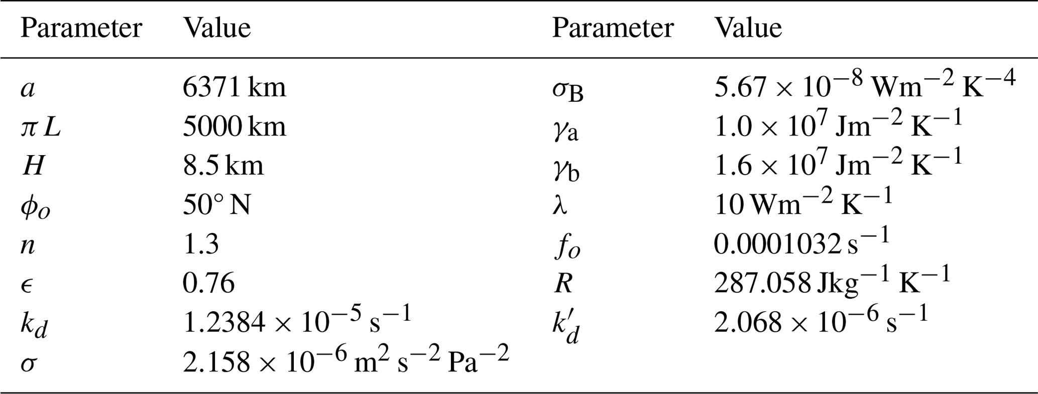
Values of λ,n, and k_d are varied beyond the displayed value to study the model sensitivity.

2.3 Model trajectories and mean fields

Figure 1 displays the time evolution of the first barotropic (ψ_a,1) and baroclinic (θ_a,1) streamfunction modes of the atmosphere and the ground temperature (T_g,1) for about 10 years starting after 10 000 d of transient integration. Fluctuations are more erratic in the atmospheric part, which denotes its key role in the dynamics of the system. The variable representing the land component of the system is comparatively slower and less erratic. This difference suggests that the land component has a longer typical timescale than the atmosphere in this system.

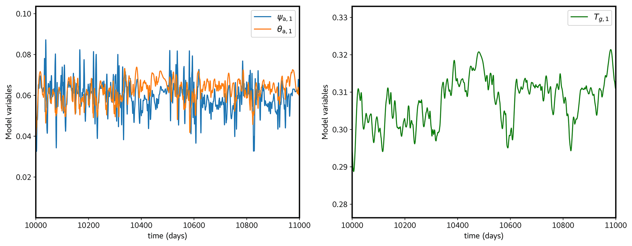
Figure 1 Temporal evolution of the barotropic (ψ_a,1) and baroclinic (θ_a,1) atmospheric streamfunction and the ground temperature (T_g,1) for C_g=300 Wm⁻² and k_d=0.085.

Figure 2a emphasizes the observation above, where the autocorrelation of the first barotropic atmospheric mode and the first ground temperature mode for C_g=300 Wm⁻² and k_d=0.085 are displayed. These, evaluated on a time series of 10 000 d, helps us estimate the memory loss of the variables.

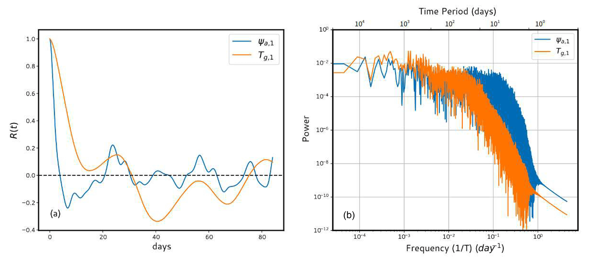
Figure 2 (a) Autocorrelation of the barotropic (ψ_a,1) atmospheric streamfunction and the ground temperature (T_g,1) for C_g=300 Wm⁻² and k_d = 0.085. (b) Power spectrum of the same variables.

Indeed, the typical timescale of the processes at hand can be evaluated by the e-folding time, which is the time beyond which the correlation has decreased by $\mathrm{1}/e$. As expected the e-folding time of the atmospheric part is approximately 1.9 d, which is comparatively lower than that of the land part (≈ 7.6 d), indicating that the system is a multiscale model with a typical timescale ratio of 10 for the specific parameter values considered.

Figure 2b depicts the power spectra of modes ψ_a,1 and T_g,1 calculated by the Fourier transformation of the autocorrelation function again using time series of 10 000 d. The atmospheric mode has a flat spectrum for lower frequencies and decays rapidly for higher frequencies. The spectrum for the ground mode initially follows the path of the atmosphere (lower frequencies up to 0.001) but starts to decay earlier, which indicates more structured variabilities at lower frequencies than the atmosphere. The existence of a substantial continuous part in the spectrum is an indication of the complexity of the deterministic dynamics in time and suggests the presence of chaotic dynamics (Arbabi and Mezić, 2017; Mezić, 2020).

3 Methodology

The objective of this research – besides introducing the basic equations as well as energy balance scheme and its sensitivity – is to explore the predictability of blocking and zonal weather regimes. By analyzing the peculiarities and the patterns of the land–atmospheric coupled model, the study concludes that, when utilizing the parameters described in Sect. 2.2, the system shows a qualitatively similar behavior as the large-scale actual atmosphere at midlatitudes (examples are illustrated in Appendix B). Moreover, varying the surface friction term, k_d, within the range of 0.06 to 0.12 yields numerous instances of realistic flow regimes, including blocking, zonal, and transition phases between these two states. To isolate these flow regimes, a machine learning algorithm called Gaussian mixture clustering (GMC) is employed, which is described in Appendix A. After classifying the data, the average geopotential height at 500 hPa of each cluster is calculated to identify different flow regimes. Through experimentation encompassing two to six clusters, discernible flow regimes emerged for two and three clusters, showcasing significant distinctions. However, as the cluster count reached four, we noted convergence between two clusters, leading to identical structures and flow patterns. This trend persisted with additional cluster increments. Hence, we inferred that the attractor attained optimal clustering with evident and nearly uniform data point distribution when employing three clusters. Each flow regime is equally important due to its presence in the actual atmosphere. The cluster containing the lowest fraction of points in percentage is designated as the transition regime. The predictability horizon of each regime is evaluated by computing the inverse of the average largest local Lyapunov exponents of the clusters, which are calculated at each point of the attractor before clustering. Although the attractor exhibits multiple positive Lyapunov exponents, our investigation focused solely on the first exponent, as it governs the dynamics of the error and is therefore considered the most influential.

4 Regime stability and Lyapunov properties of the low-order land–atmospheric coupled model

The instability properties of different flow regimes and their dependence with respect to important parameters are investigated as follows: the first part explores the sensitivity of the model to essential parameters which play a key role in structuring the output of the system. In the second part, the predictability properties of zonal, blocking, and transition flow regimes using the Lyapunov exponents are investigated.

4.1 Stability properties of the model

Stability properties of the land–atmosphere coupled model at their equilibrium states are well depicted in Li et al. (2018). They also defined high-index equilibria and low-index equilibria based on the value of the streamfunction in the upper- and lower-atmospheric layer when the model solutions are equilibrium states. Even though the stability of the model's equilibrium states is interesting and insightful, the actual atmosphere displays time-dependent solutions. Moreover, realistic atmospheric models are chaotic and acutely sensitive to the initial conditions. Hence in this section, we investigated the stability properties of the land–atmosphere model when its behavior is similar to Earth-like situations with erratic dynamics.

Chaotic dynamical systems which exhibit sensitivity to the initial conditions can be qualitatively analyzed by computing Lyapunov exponents and vectors.

4.2 Theory

Sensitivity to initial conditions is usually estimated using Lyapunov exponents. Let us consider an initial state, x(t_o)=x_o: a small perturbation δx_o is added to it, which eventually produces a completely different trajectory. The dynamics of the error growth of the system can be linearized provided the perturbation is infinitesimally small as

$$\begin{array}{}\text{(6)}& {\displaystyle \frac{\mathrm{d}\mathit{\delta }\mathit{x}}{\mathrm{d}t}}={\left.{\displaystyle \frac{\partial \mathit{f}}{\partial \mathit{x}}}\right|}_{\mathit{x}\left(t\right)}\mathit{\delta }\mathit{x}\end{array}$$

and its solution is

$$\begin{array}{}\text{(7)}& \mathit{\delta }\mathit{x}\left(t\right)=\mathbf{M}(t,\mathit{x}(t_o\left)\right)\mathit{\delta }\mathit{x}\left(t_o\right),\end{array}$$

where M is known as the resolvent or propagator matrix. The Euclidean norm of the error can be computed as

$$\begin{array}{}\text{(8)}& \begin{array}{rl}& E_t=\left|\mathit{\delta }\mathit{x}\right(t){|}^{\mathrm{2}}=\mathit{\delta }\mathit{x}(t{)}^T\mathit{\delta }\mathit{x}\left(t\right)\\ & E_t=\mathit{\delta }\mathit{x}\left(t_o{)}^T\mathbf{M}\right(t,\mathit{x}\left(t_o\right){)}^T\mathbf{M}(t,\mathit{x}(t_o\left)\right)\mathit{\delta }\mathit{x}\left(t_o\right),\end{array}\end{array}$$

hence indicating that the error growth is provided by the eigenvalues of M^TM, where M^T denotes the transpose of the resolvent matrix M. By the multiplicative ergodic theorem of Oseledec (Eckmann and Ruelle, 1985; Kuptsov and Parlitz, 2012), a double limit is considered with perturbation amplitude going to 0 and time going to infinity. The logarithm of the eigenvalues of matrix $({\mathbf{M}}^T\mathbf{M}{)}^{\mathrm{2}(t-t_o)}$ within these limits, which are known as Lyapunov exponents, quantifies the divergence of the initially close trajectories. The complete set of Lyapunov exponents that are usually represented in decreasing order constitutes the Lyapunov spectrum. Different types of Lyapunov vectors exist based on the method of calculation like forward Lyapunov vectors, backward Lyapunov vectors, and covariant Lyapunov vectors, whose properties are described in detail in Kuptsov and Parlitz (2012) and Legras and Vautard (1996).

In the current study, we are using backward Lyapunov vectors (BLVs), which are obtained by considering the eigenvalues of the matrix $({\mathbf{M}}^T\mathbf{M}{)}^{\mathrm{2}(t-t_o)}$ by taking initial state $t_o\to -\mathrm{\infty }$. Several numerical techniques exist for the calculation of the Lyapunov exponents. The most common method is using Gram–Schmidt orthonormalization (Shimada and Nagashima, 1979; Parker and Chua, 2012): a set of orthonormal random vectors are propagated in the tangent space of the trajectory, according to Eq. (6), frequently re-orthonormalizing this basis to avoid the collapse of all the vectors towards the most unstable direction which is associated with the largest Lyapunov exponent. After a transient, these vectors provide the BLVs and concurrently the sought Lyapunov exponents. As mentioned in Sect. 2.1, Lyapunov exponents computed here consider both spatial and temporal chaos. The complete set of these vectors give the full picture of the instability of the trajectory in phase space.

4.3 Lyapunov spectra and averaged variance of the model

Figure 3 displays the Lyapunov spectrum of the land–atmosphere coupled model when C_g=300 Wm⁻² and k_d=0.085. All other parameters are provided in Table 1. The system has 3 positive, 1 zero, and 26 negative Lyapunov exponents. Similar to the ocean–atmospheric coupled model (Vannitsem et al., 2015; Vannitsem and Lucarini, 2016; Vannitsem, 2017), the spectrum contains a set of Lyapunov exponents forming a plateau close to 0, but the amplitude of the Lyapunov exponents around this plateau is quite substantial compared to the coupled ocean–atmosphere model. This plateau is expected to be associated with the presence of the land, whose typical timescales of variability are slower than the atmosphere.

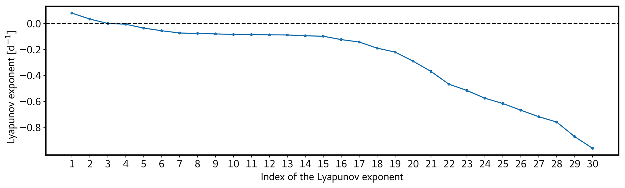
Figure 3 Lyapunov spectra of the land–atmospheric coupled model for C_g=300 Wm⁻² and k_d=0.085. The values of the Lyapunov exponents are given in d⁻¹.

The coupling between the land and atmosphere plays a key role in the behavior of the model. Hence quantifying the extent of this coupling and its instabilities is essential for interpreting the properties of the model. Therefore, the averaged variance of the Lyapunov vectors is displayed in Fig. 4 to elucidate this information along each variable.

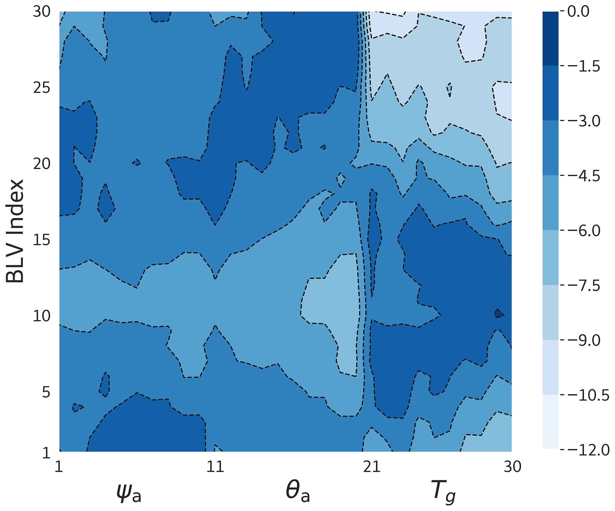
Figure 4 Values of the time-averaged and normalized variance of the BLVs as a function of the variables of the model (log₁₀ scale). The first 20 modes correspond to the variables of the atmosphere and the next 10 correspond to the temperature of the ground. Parameter values: C_g=300 Wm⁻² and k_d=0.085. The Euclidean norm is used for all BLVs, and their squared norm is normalized to 1.

The first 10 variables represent the barotropic streamfunction of the atmosphere, the next 10 represent the baroclinic streamfunction of the atmosphere, and the last 10 represent the ground temperature. The variance of the BLVs is primarily in the atmospheric part, indicating that this part primarily contributes to the system's dynamics. It should also be noted that the atmospheric part includes the most unstable BLVs (corresponding to the first two Lyapunov exponents) as well as the most stable BLVs (21 to 30 correspond to large negative Lyapunov exponents – LEs).

Conversely, variance is predominantly projected on the temperature variables of the ground part for BLVs 3 to 20. These BLVs are associated with the plateau formed by the near-zero LEs visible in Fig. 3. The observation of comparable variance in both the atmospheric and ground parts describes (horizontally) the coupling in the model, which is thus represented for BLVs 3–7. For BLVs 21 to 30, variance projection is almost nonexistent in the ground part, indicating that the ground part makes almost no contribution to the stabilization of the system.

Figure 5 displays Lyapunov spectra calculated for various energy input levels (C_g) ranging from 300 to 400 Wm⁻².

When C_g is lower, the model exhibits chaotic behavior, indicated by 2 positive exponents, 1 zero exponent, and 26 negative exponents. Surprisingly, the amount of incoming shortwave radiation does not significantly affect the spectrum between C_g values of 300 and 360 Wm⁻².

However, as C_g increases, the system shifts to periodic behavior, characterized by 1 zero exponent and 29 negative Lyapunov exponents, before switching back to chaos.

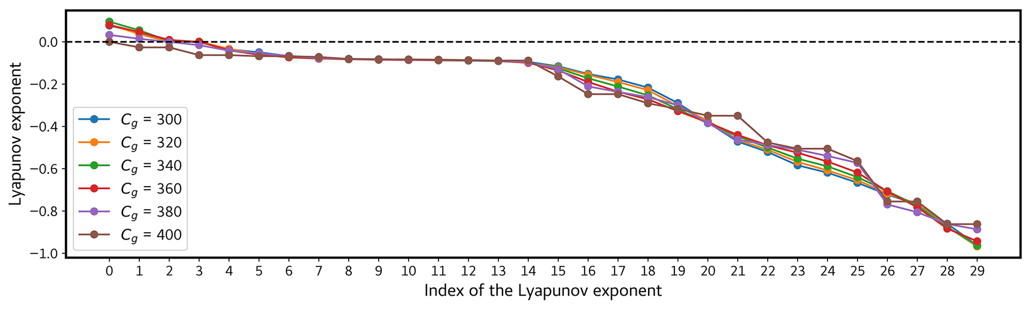
Figure 5 Lyapunov spectra of the land–atmospheric coupled model for different values of C_g. Each color represents corresponding C_g values used for calculating the spectrum. The values of the Lyapunov exponents are given in d⁻¹.

This is illustrated in Figure 6 where the first and second Lyapunov exponents are positive for the system for the lower values of C_g, and then the system enters a periodic window for the C_g values and reverts back to chaotic behavior again later.

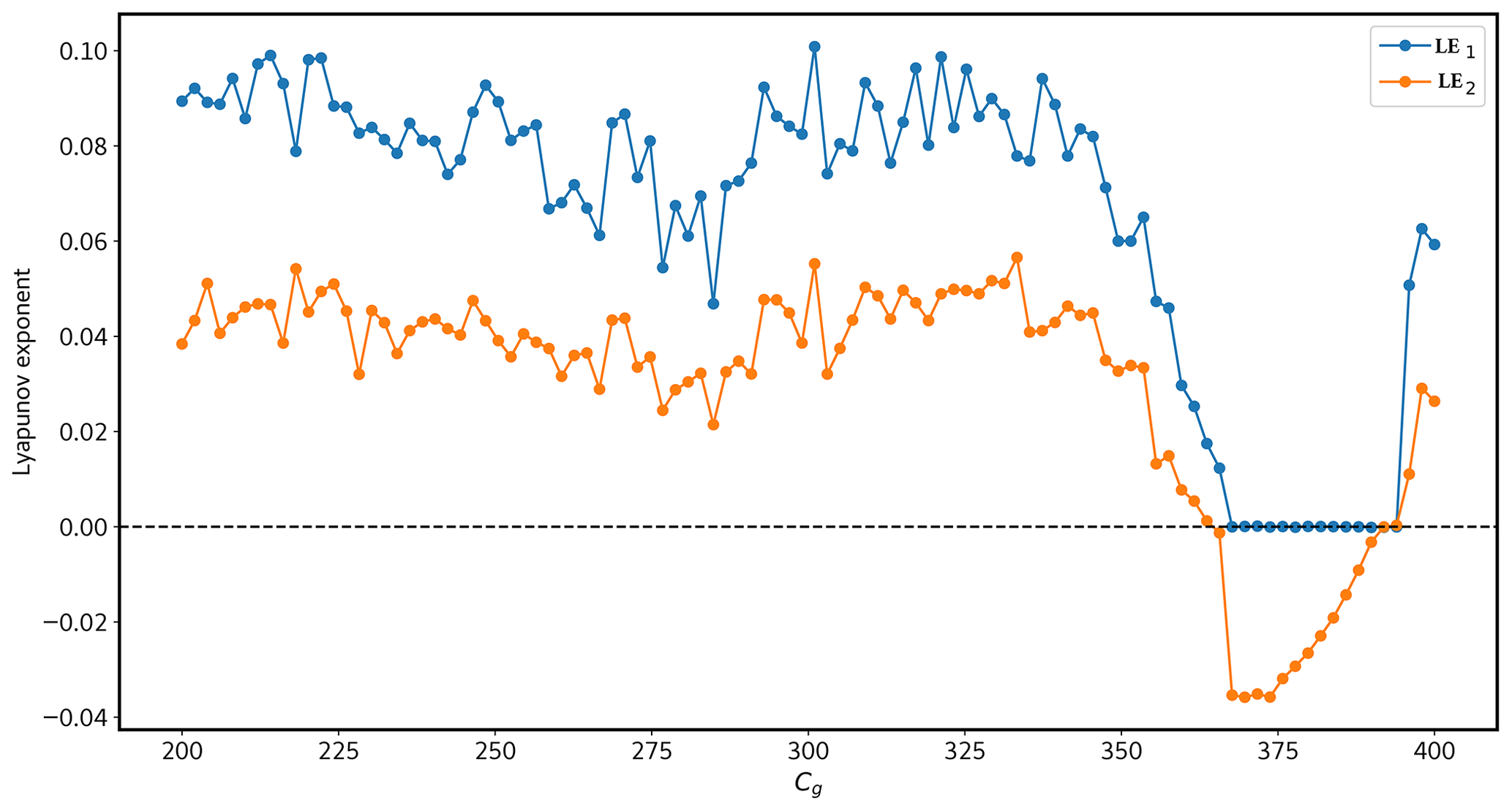
Figure 6 First and second Lyapunov exponents of the land–atmospheric coupled model for different values of C_g for a fixed value of k_d=0.08. The blue line represents the first and the orange line represents second Lyapunov exponents, respectively. The values of the Lyapunov exponents are given in d⁻¹.

The surface friction k_d also affects the stability of the system to a great extent. In order to investigate the sensitivity of the model to k_d, Lyapunov spectra were drawn with the parameter values exhibited in Table 1 with different k_d values as displayed in Fig. 7.

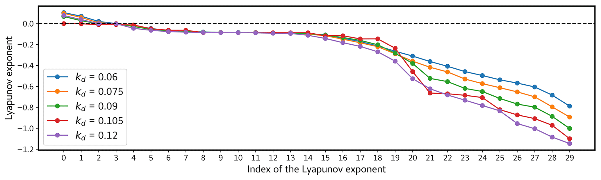
Figure 7 Lyapunov spectra of the land–atmosphere coupled model for different values of k_d. Each color represents corresponding k_d values used for calculating the spectrum. The values of the Lyapunov exponents are given in d⁻¹.

The nondimensional k_d values depicted in the figure were obtained from Reinhold and Pierrehumbert (1982), where they asserted that flow regimes generated using these values exhibit realistic midlatitude terrestrial properties. Among the system configurations with k_d values of 0.06, 0.075, 0.09, and 0.12, there are 3 positive, 1 zero, and 26 negative Lyapunov exponents. Up to the point of plateau formation, all these spectra display similar behavior. Note that the spectrum corresponding to k_d=0.12 exhibits notably strong negative Lyapunov exponents, while the spectrum for k_d=0.06 demonstrates comparatively weaker negative values, as expected from the increased associated dissipation.

From Fig. 4, we identify BLVs 20–30 as actually depicting the variance of the temperature of the atmosphere. Given the significant variation in BLVs 20–30 within the current context, it can be inferred that the atmospheric temperature gradient, and hence baroclinic instability, is becoming weaker and the system is stabilizing due to the changes in the surface friction.

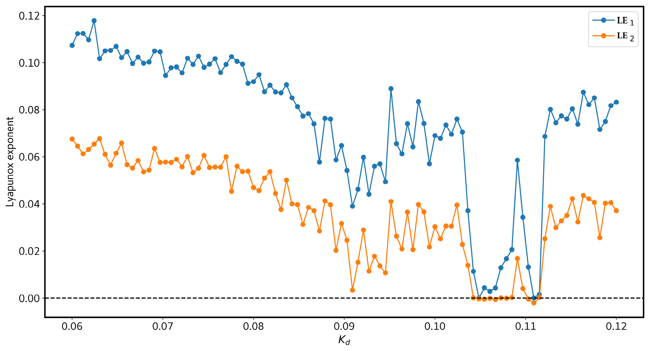
Figure 8 First and second Lyapunov exponents of the land–atmosphere coupled model for different nondimensional values of k_d. The blue line represents the first and the orange line represents the second Lyapunov exponents, respectively. C_g=300 Wm⁻². The values of the Lyapunov exponents are given in d⁻¹.

As thoroughly explained in Sect. 4.2, the largest Lyapunov exponent serves as an indicator of the system's highest degree of instability, while the second positive Lyapunov exponent represents the second-most unstable characteristic, and so forth. In Fig. 8, the results demonstrate that at lower values of k_d, the system exhibits a highly chaotic nature. However, as we increase k_d towards higher values, the system stabilizes, revealing a periodic window. This can also be seen with the Lyapunov spectrum for k_d=0.105 in Fig. 7.

Subsequently, with further increment in k_d, the system returns to a more chaotic behavior, illustrating the complex role of dissipative features.

The primary interaction between the land and atmosphere in the model is facilitated through heat exchange denoted by λ. Therefore, it is crucial to understand and analyze how alterations in the heat exchange mechanism influence the behavior of the model. This is illustrated in Fig. 9.

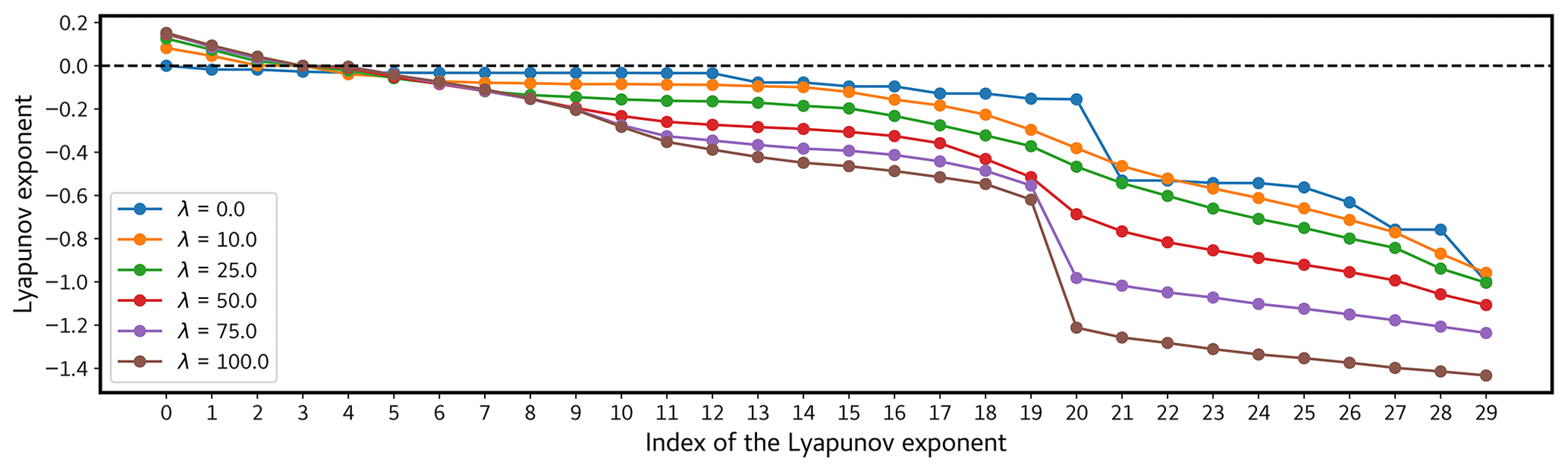
Figure 9 Lyapunov spectra of the land–atmospheric coupled model for different values of λ. Each color represents corresponding λ values used for calculating the spectrum. The values of the Lyapunov exponents are given in d⁻¹.

When λ is set to zero, the system displays a periodic behavior characterized by 1 zero and 29 negative Lyapunov exponents. However, for all other nonzero λ values, the system exhibits chaos with 3 positive exponents, 1 zero exponent, and 26 negative Lyapunov exponents. Smaller values of λ (e.g., λ=10, 25, and 50) yield a smooth spectrum with a plateau which is similar to the typical Lyapunov spectrum encountered before. Note that with higher λ values, an anomalous bend is observed in the spectrum, specifically from the 20th exponent onward, indicating unrealistic stability. It is also interesting to note that the spectrum associated with the intersection of the land part (between the 20th and 21st exponent) becomes steeper with the increase in λ. The increased heat exchange leads to a reduced temperature difference between the atmosphere and the ground, thereby giving rise to this particular situation. This can be further explained by the averaged variance of Lyapunov exponents for different values of heat exchange λ in Fig. 10.

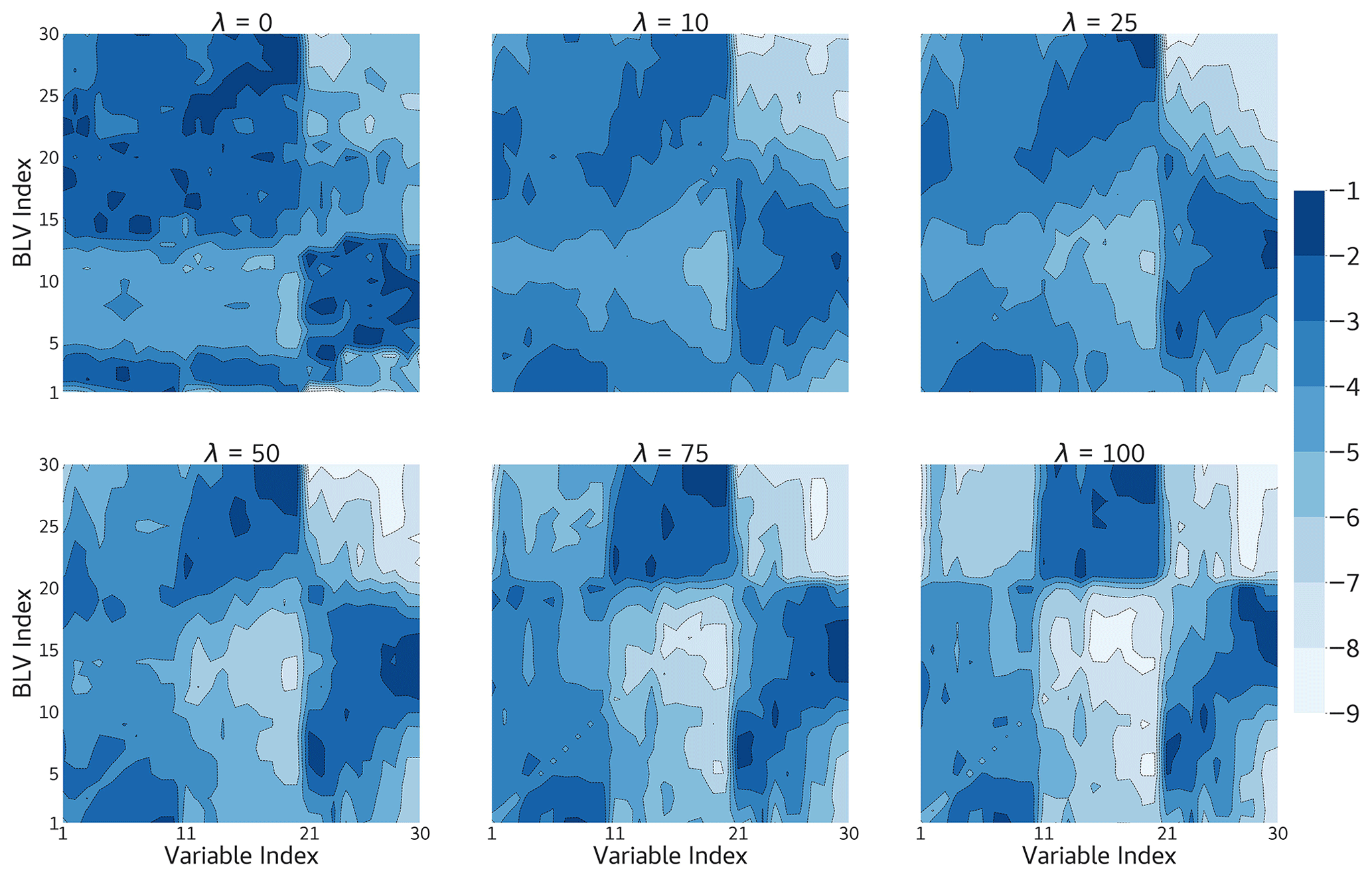
Figure 10 Values of the time-averaged and normalized variance of the BLVs as a function of the variables of the model (log₁₀ scale) for different λ values in Wm⁻² K⁻¹. The first 20 modes correspond to the variables of the atmosphere and the next 10 correspond to the temperature of the ground. Parameter values: C_g=300 Wm⁻² and k_d=0.085. The Euclidean norm is used for all BLVs, and their squared norm is normalized to 1.

A clear separation between the land and atmosphere exists at λ=0, when there is no exchange of heat between them, resulting in the respective spectrum. For λ=10, 25, and 50, the distribution remains similar, with variances concentrated predominantly in the atmospheric component for the first 3 BLVs and the last 10 BLVs. BLVs 3–20 represent a plateau-like pattern, indicating a coupling between the atmosphere and the ground. Despite variance distribution, it is notable that there is a uniform spread rather than a strong concentration or absence of variance. For λ=75 and 100, the variance distribution becomes compartmentalized. Variance is now concentrated within the first 20 BLVs for the barotropic streamfunction and ground temperature, while the last 10 BLVs primarily represent atmospheric temperature or the baroclinic streamfunction. In contrast to earlier cases, there is a clear absence of variance within the middle portion, specifically confined to BLVs 20–30. This compartmentalized energy distribution leads to a characteristic jump in the corresponding spectrum.

5 Predictability properties of zonal, blocking, and transition flow regimes

Upon concluding our investigation of the land–atmosphere coupled model's utility in studying low-frequency variability in the atmosphere, we have identified zonal, blocking, and transition regimes concerning different k_d values, as explained in Sect. 3. For the range of k_d values between 0.06 and 0.12, the lower values (0.06 to 0.075) encompass all three regimes: zonal, blocking, and transition. As we progress from 0.08 onward, we observe two blocking regimes and a transitional regime between them until k_d=0.10. Subsequently, the system exhibits periodic behavior. At k_d=0.115, two blocking regimes are observed, and further, at k_d=0.12, three flow regimes are identified. These findings demonstrate the model's capability to capture various flow regimes and their transitions based on the selected range of k_d values.

The predictability horizon of the zonal regimes is found to be longer compared to the blocking regimes in the range of k_d values where all three regimes coexist (k_d=0.06 to 0.075). This implies that the blocking regimes exhibit higher instability, in agreement with previous findings (Schubert and Lucarini, 2016; Faranda et al., 2016, 2017; Lucarini et al., 2016). The transition regimes, on the other hand, show notably lower predictability in comparison to the other regimes. Within the interval of k_d values encompassing only two blocking regimes and a transition regime (k_d=0.08 to 0.10), both blocking regimes display significantly different predictability horizons. At the outset (k_d=0.08), they demonstrate a predictability difference of approximately 1 d. Subsequently, this difference increases and reaches about 10 d at k_d=0.095. However, it then decreases again to a difference of 1 d when k_d=0.10. Moreover, it is observed that the stability of the transition regime surpasses that of one of the blocking regimes. This indicates the occurrence of a qualitative change in the predictability of the blocking regimes within this particular range of k_d values.

In these instances, it is noteworthy that situations characterized by lower predictability or significant instability tend to occur when atmospheric blocking takes place on the western side of topographical features. Conversely, when blocking occurs on the eastern side of such topography, it exhibits greater stability and a longer predictability horizon. This observation draws parallels with real-world scenarios, such as the persistence of North Pacific blocking patterns (Breeden et al., 2020; Kim and Kim, 2019). The morphology of the identified blocking events bears resemblance to North Pacific blocks, where a high-pressure system is situated either to the west or east of the underlying topography. These locations correspond to the windward and leeward sides of the mountain ranges in the model.

The system enters a periodic window after k_d=0.10. Then it again becomes chaotic with two blocking regimes and a transition regime and later on with three distinct regimes. Figure 11 depicts all the findings obtained from this study.

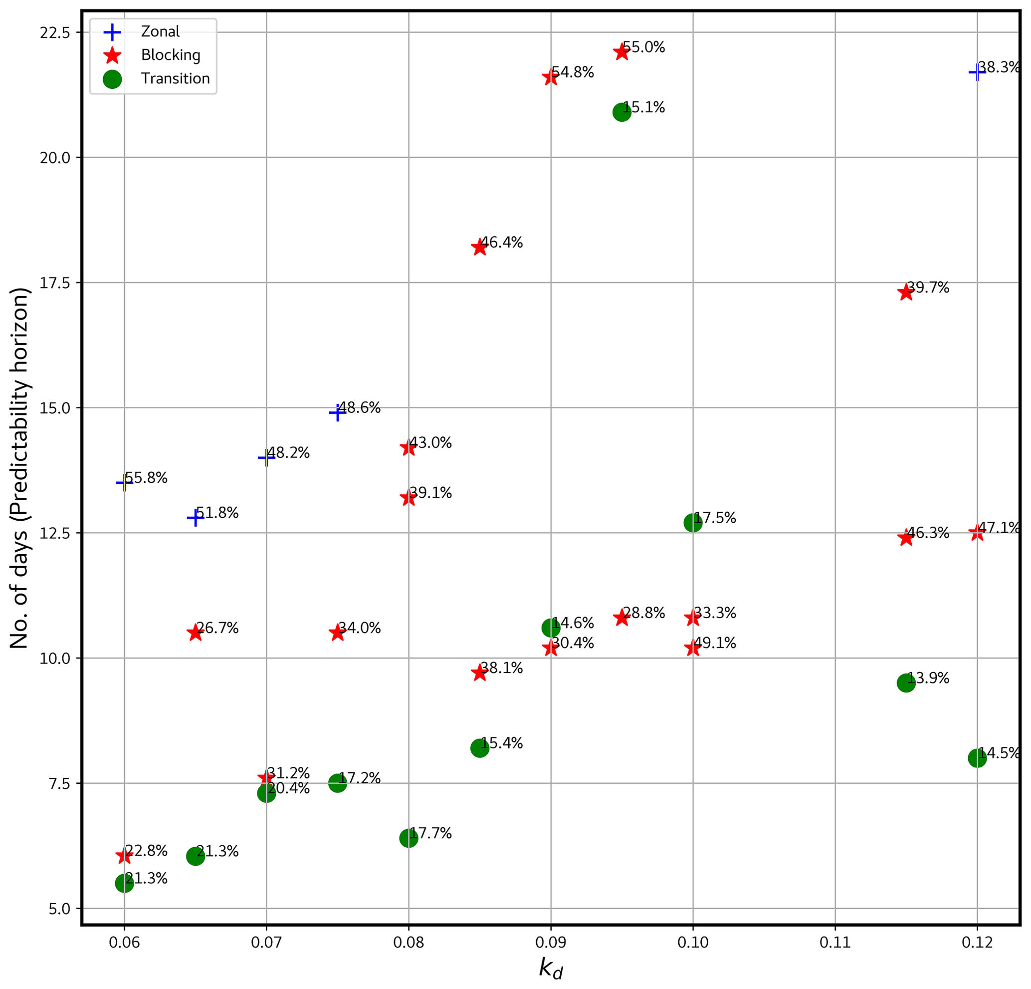
Figure 11 Predictability horizon of zonal, blocking, and transition flow regimes for different nondimensional k_d. The numbers represent the percentage of the total number of points included in the respective regime. The predictability horizon is depicted in days.

6 Impact of model resolution

As per Cehelsky and Tung (1987), the resolution of the model can affect the output in various ways. For instance, the nonlinear interaction between the modes (as the number of modes increases, the resolution of the system increases) is quite altered if different number of modes are considered, resulting in entirely different dynamics for the same set of parameters. Hence, analysis of high-resolution runs and their Lyapunov properties is inevitable. In this section, the system is run with a higher-resolution configuration (5,5) with 55 modes being used for both the atmospheric and land part, giving a system with a total of 165 variables. Parameter values are the same as those of the earlier analysis listed in Table 1. Figure 12 depicts the Lyapunov spectrum and Fig. 13 represents the time-averaged variance of the BLVs of the high-resolution run.

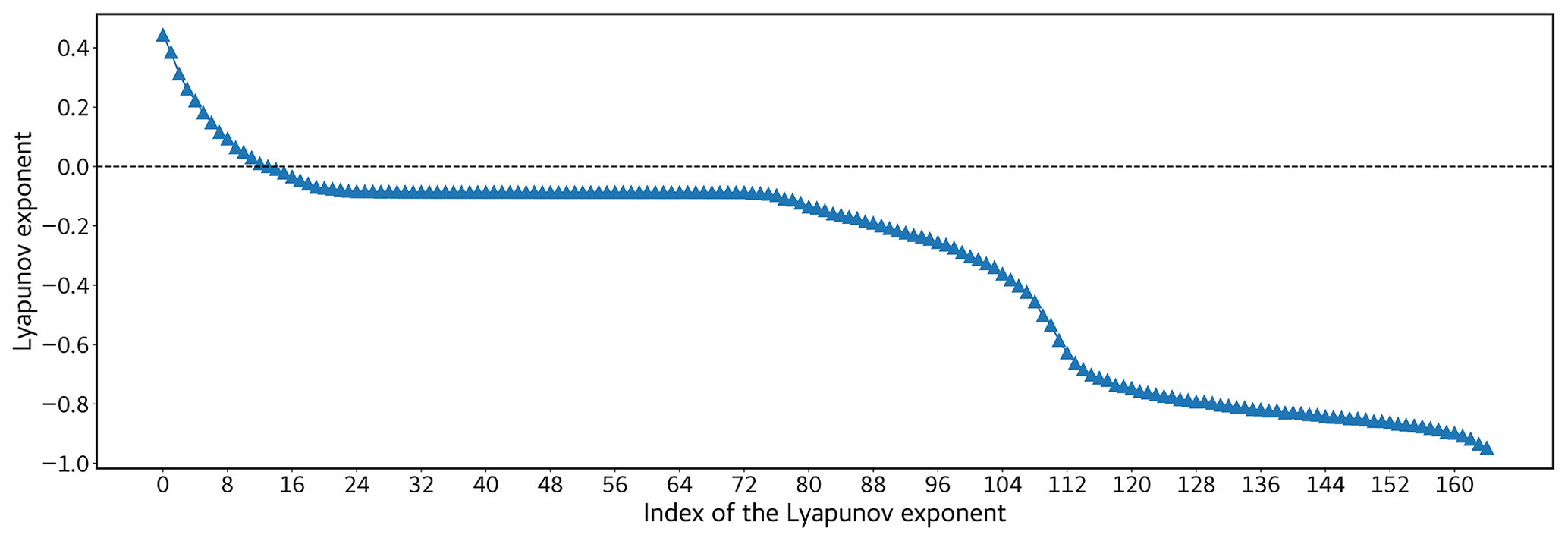
Figure 12 Lyapunov spectrum of the land–atmosphere coupled model for C_g=300 Wm⁻² and k_d=0.085 in (5,5) model configuration. The values of the Lyapunov exponents are given in d⁻¹.

The Lyapunov spectrum exhibits structural similarity when compared to the low-resolution spectra, except that more positive exponents are present. Specifically, it comprises 12 positive, 1 zero, and 152 negative exponents. Notably, there is a distinctive plateau observable within the range of 20 to 75, which is a characteristic feature attributed to the interaction between the land and the atmosphere in the model. This plateau phenomenon arises due to the disparity in timescales resulting from the intricate interplay between land and atmosphere dynamics.

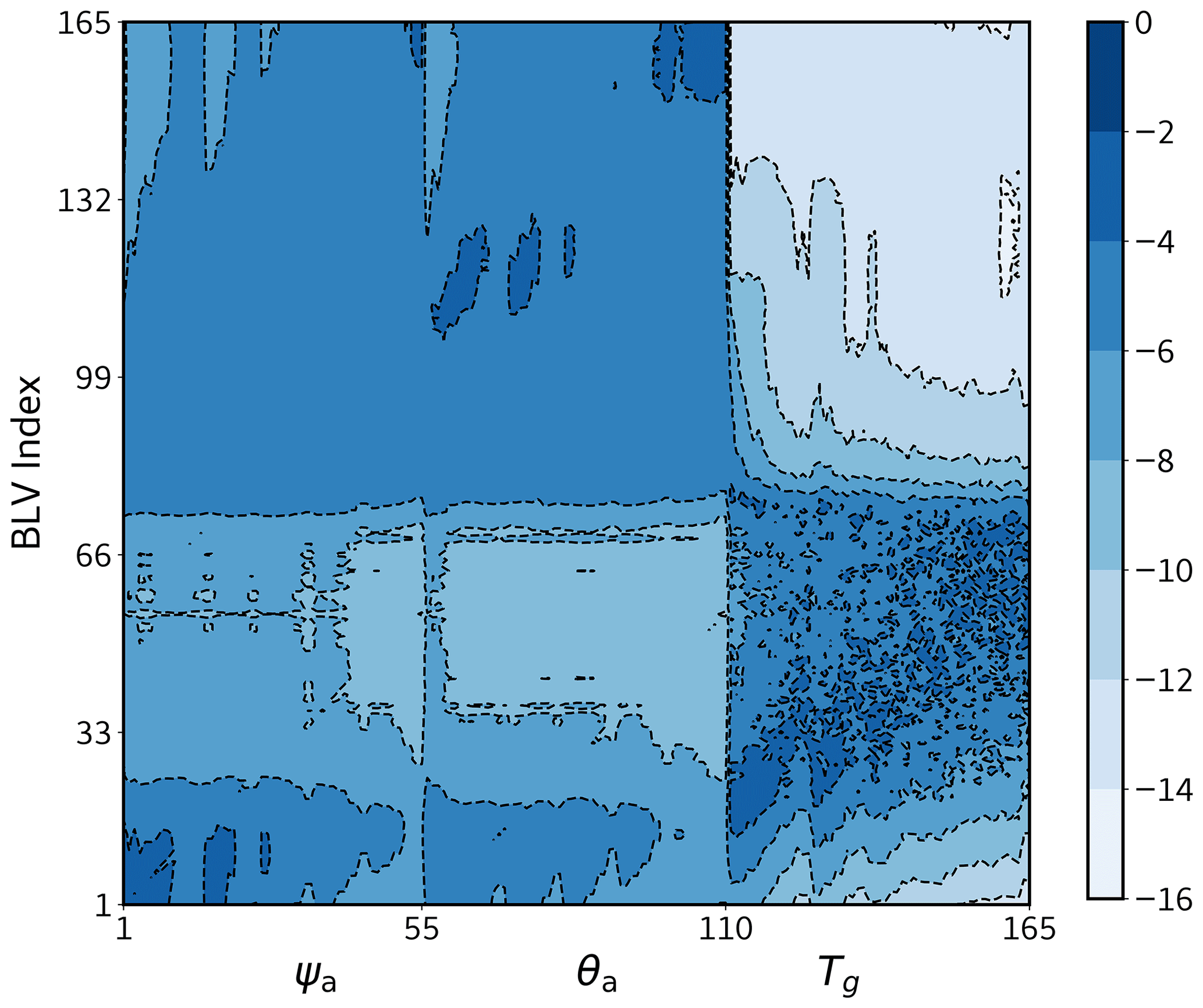
Figure 13 Values of the time-averaged and normalized variance of the BLVs as a function of the variables of the model (log₁₀ scale) in (5,5) model configuration. The first 110 modes correspond to the variables of the atmosphere and the next 55 correspond to the temperature of the ground. Parameter values: C_g=300 Wm⁻² and k_d=0.085. The Euclidean norm is used for all BLVs, and their squared norm is normalized to 1.

In Fig. 13, higher variances in the atmosphere are observed for the first 40 BLVs and also for the BLVs greater than 70, indicating that the most chaotic and stable dynamics result from the atmospheric component. Furthermore, it is noteworthy that a greater concentration of variance is observed to be shifted towards the variables that specifically represent the ground temperature, particularly within the range of BLVs 20 to 75. This shift is a key factor contributing to the formation of a plateau within the spectrum in question. It becomes evident that there is a distinct compartmentalization between each set of variables, including the barotropic, baroclinic, and ground temperature variables, which is more pronounced when compared to the variance illustration at lower resolutions.

The outcome of the clustering analysis has identified two clearly defined patterns: one marked by zonal flow and the other by instances of blocking. The intermediate pattern that once existed between these two regimes is now absent. Notably, both the zonal and blocking events exhibit an identical predictability horizon, specifically spanning a period of 2 d. This feature contrasts with what is found at the lower resolution and also in the current literature on this topic. This aspect is worth investigating further in the future by exploring other sets of parameters and other resolutions.

7 Discussion

This study focuses on characterizing the variability and instability properties of different flow regimes and their dependence on important parameters in an idealized coupled model, namely the quasi-geostrophic land–atmosphere coupled model. The investigation also aims to explore the predictability of zonal, blocking, and transition flow regimes using Lyapunov exponents.

The analysis revealed that the model is less sensitive to variations in meridional differences in solar heating absorbed by the land, represented by C_g. Based on observations, a fixed value of 300 Wm⁻² for C_g was chosen for further analysis. The study found that the model's stability is significantly affected by surface friction k_d. Different values of k_d were explored, and it was observed that at lower k_d values, the system exhibits chaotic behavior, while at higher k_d values, periodic windows alternate with chaotic behaviors. Within this range, the system solutions meander between various flow regimes, including zonal, blocking, and transition.

The heat exchange mechanism, represented by λ, was also analyzed, and it was found that when λ is set to zero, the system displays periodic behavior, while for nonzero λ values, the system exhibits considerable chaos. Overall, the model demonstrated the capability to capture various flow regimes and their transitions based on the selected range of k_d values, providing insights into the potential behavior of the atmosphere.

The predictability properties of three distinct flow regimes were investigated: zonal, blocking, and transition, which were the fundamental components of low-frequency variability (LFV) in the model. The predictability horizon of the zonal regimes was found to be longer compared to the blocking regimes, which is consistent with earlier results (Schubert and Lucarini, 2016; Faranda et al., 2016, 2017; Lucarini et al., 2016), when all three regimes coexist. The transition regimes showed notably lower predictability compared to the other regimes. Within a specific range of k_d values, the blocking regimes displayed different predictability horizons, indicating the occurrence of a qualitative change in the predictability of the blocking regimes.

Weather patterns that involve atmospheric blocking to the west of a given topographical feature tend to have reduced predictability and show instability when contrasted with blocking occurrences situated to the east of such topographical elements. This finding aligns with actual meteorological occurrences, such as the persistence of North Pacific blocking patterns (Breeden et al., 2020; Kim and Kim, 2019). The shape and characteristics of the identified blocking events closely resemble North Pacific blocks, where a high-pressure system exists either on the western or eastern side of the underlying topography. In the physical world, these positions correspond to the windward and leeward sides of mountain ranges composed of rocky terrain. Despite qgs models being regarded as less comprehensive, their utilization in this study allows for a more relevant impact, akin to real-world situations as described above.

Upon increasing the model resolution, Lyapunov properties exhibited a remarkable resemblance to those observed at lower resolutions. However, the distribution of points on the attractor gave rise to two distinct clusters, delineating the blocking and zonal regimes, thereby extinguishing the potential for the transition regime. Notably, both the blocking and zonal regimes displayed a predictability horizon limited to 2 d.

Against the backdrop of rising global temperatures and the escalation of climate extremes, comprehending the intricate dynamics governing atmospheric blocking occurrences and their predictability is becoming paramount, given that blocking events are consistently linked to extreme weather phenomena. The impact of climate change can also be explored in the current study by modifying the emissivity of the atmosphere. This will be explored in the future.

The knowledge acquired through this study holds potential significance for climate and weather prediction models, contributing to the advancement of our understanding of the crucial atmospheric dynamics shaping the Earth's climate system. In future investigations, we will assess the influence of the same parameters within more complex models, enabling us to conduct comparisons that will aid in identifying alterations in land–atmosphere interactions as atmospheric complexity intensifies. This undertaking will further our comprehension of how the interaction between the land and atmosphere evolves with increasing intricacies in atmospheric systems and how it affects the predictability of weather regimes.

Appendix A: Gaussian mixture clustering (GMC)

Gaussian mixture clustering (GMC) is a prevalent unsupervised machine learning technique utilized for partitioning data points into clusters by modeling their underlying distribution. While the distribution of data points on the attractor may not align with a Gaussian distribution, the algorithm proceeds by approximating the distribution as Gaussian and subsequently identifies clusters based on this approximation. Each cluster is characterized by a Gaussian component, and the primary objective is to accurately estimate the parameters of these components to optimally describe the data. It comprises several steps.

• Initialization. GMC starts by randomly selecting K initial centers (means) μ_i for each cluster. Additionally, it initializes the covariance matrices Σ_i and the mixing coefficients π_i, which represent the probabilities of data points belonging to each cluster, where $i=\mathrm{1},\mathrm{2},\mathrm{\dots },K$. The mixing coefficients must sum up to 1, and each must be between 0 and 1.

• Expectation–maximization (EM) algorithm. GMC employs the EM algorithm (Dempster et al., 1977) to iteratively estimate the parameters of the Gaussian components. The algorithm comprises two steps, the expectation step (E-step) and the maximization step (M-step).

  • Expectation step (E-step). During this step, the algorithm computes the responsibility (γ_i,j) of each data point x_j for each cluster i. The responsibility represents the probability that data point x_j belongs to cluster i, given the current parameters. This is calculated using Bayes' theorem:

    $$\begin{array}{}\text{(A1)}& {\mathit{\gamma }}_{i,j}={\displaystyle \frac{{\mathit{\pi }}_i\cdot \mathcal{N}(x_j;{\mathit{\mu }}_i,{\mathrm{\Sigma }}_i)}{{\sum }_{k=\mathrm{1}}^K{\mathit{\pi }}_k\cdot \mathcal{N}(x_j;{\mathit{\mu }}_i,{\mathrm{\Sigma }}_i)}},\end{array}$$

    where γ_i,j is the responsibility of cluster i for data point x_j, and π_i is the mixing coefficient for cluster i. μ_i and Σ_i are the mean and covariance matrix for cluster i, respectively. $\mathcal{N}(x_j;{\mathit{\mu }}_i,{\mathrm{\Sigma }}_i)$ is the Gaussian probability density function for data point x_j with mean μ_i and covariance Σ_i.
    

  • Maximization step (M-step). In this step, the algorithm updates the parameters of the Gaussian distributions (mean, covariance, and mixing coefficients) based on the responsibilities calculated in the E-step.

    $$\begin{array}{}\text{(A2)}& {\displaystyle }\text{New mean },{\mathit{\mu }}_i={\displaystyle \frac{{\sum }_{j=\mathrm{1}}^N{\mathit{\gamma }}_{i,j}\cdot x_j}{{\sum }_{j=\mathrm{1}}^N{\mathit{\gamma }}_{i,j}}}\text{(A3)}& {\displaystyle }\begin{array}{rl}& \text{New covariance matrix },{\mathrm{\Sigma }}_i\\ & ={\displaystyle \frac{{\sum }_{j=\mathrm{1}}^N{\mathit{\gamma }}_{i,j}\cdot (x_j-{\mathit{\mu }}_i)\cdot (x_j-{\mathit{\mu }}_i{)}^T}{{\sum }_{j=\mathrm{1}}^N{\mathit{\gamma }}_{i,j}}}\end{array}\text{(A4)}& {\displaystyle }\text{New mixing coefficient },{\mathit{\pi }}_i={\displaystyle \frac{\mathrm{1}}{N}}\sum _{j=\mathrm{1}}^N{\mathit{\gamma }}_{i,j}\end{array}$$

    N is the number of data points. μ_i, Σ_i, and π_i are the updated mean, covariance matrix, and mixing coefficient for cluster i, respectively. γ_i,j is the responsibility of cluster i for data point x_j (computed in the E-step). x_j is the jth data point.

• Convergence. The E-step and M-step are repeated iteratively until the algorithm converges. Convergence happens when the change in the likelihood of the data between iterations becomes very small or when a predefined number of iterations is reached.

• Cluster assignment. Once the algorithm converges, each data point is assigned to the cluster with the highest probability (highest responsibility).

• Number of clusters (K). The number of clusters, K, is typically determined either by the user based on prior knowledge or by using techniques like the Bayesian information criterion (BIC) or cross-validation to find the optimal number of clusters.

In our study, we used the cross-validation method and decided K should be 3 for obtaining realistic results. Further explanation regarding the clustering algorithm can be obtained from recent literature on that subject (Hastie et al., 2009; Bishop and Nasrabadi, 2006; Dempster et al., 1977; Smyth et al., 1999).

Appendix B: Examples of blocking and zonal patterns evolved from the study

As previously indicated, employing the parameter configuration outlined in Table 1, we have successfully generated Earth-like flow patterns. These flow regimes are visually represented in Figs. B2 and B1, corresponding to different values of the parameter k_d. Specifically, for lower values of k_d, we observe the coexistence of zonal, blocking, and transitional flow regimes, as depicted in Fig. B1. Conversely, when k_d assumes higher values, we observe the emergence of two blocking flow regimes along with a transition regime, as illustrated in Fig. B2.

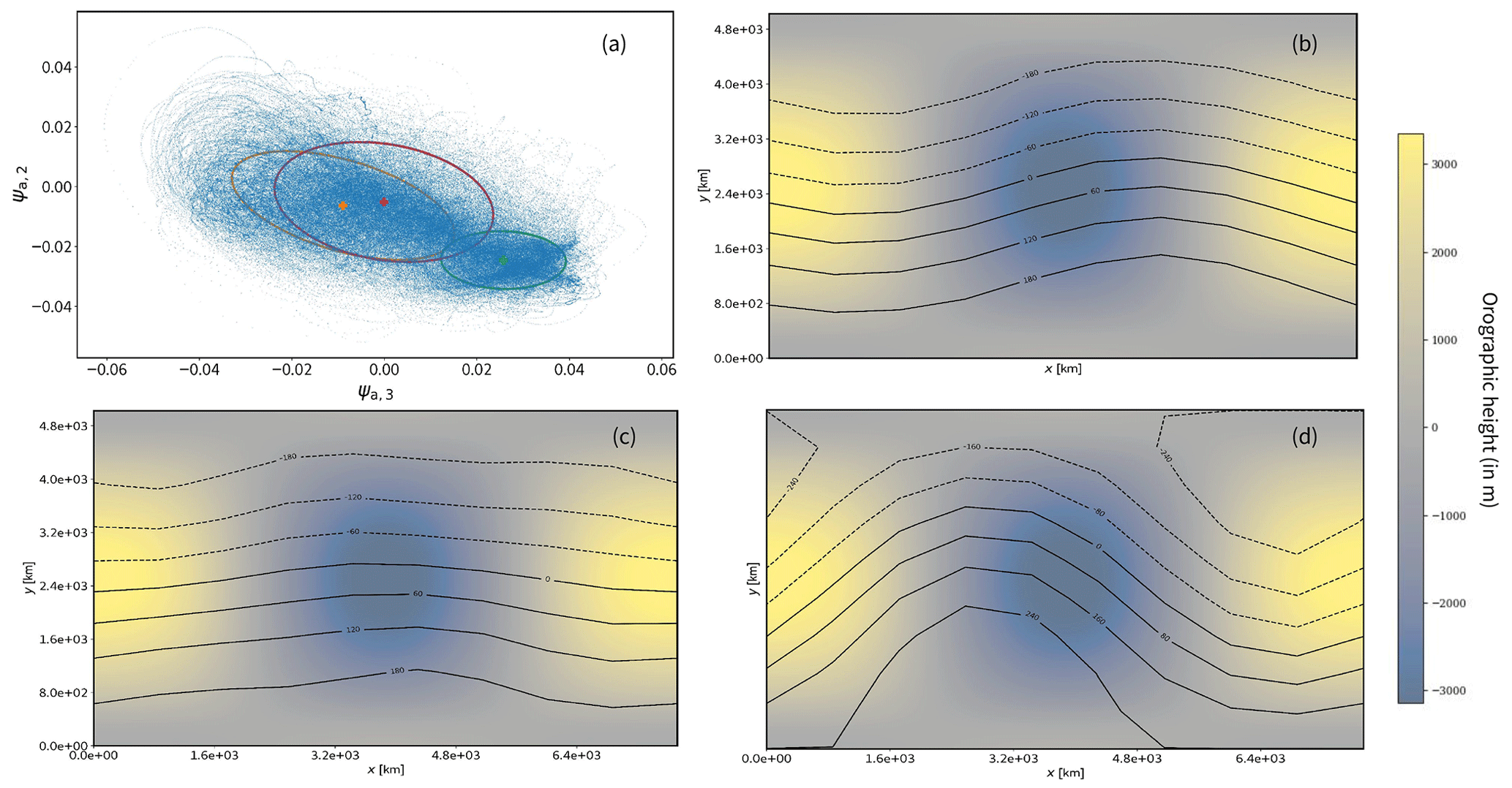
Figure B1 The phase space dynamics of the model projected on the (ψ_a,3, ψ_a,2) plane (a) for k_d = 0.065 . Gaussian mixture cluster covariances are represented with orange, green, and red ellipsis. The orange cluster is associated with a zonal regime which can be identified by the geopotential height at 500 hPa in panel (b). Red and green clusters are respectively transition and blocking regimes in panel (c) and (d), also at 500 hPa geopotential height. The orographic profile of the domain is depicted in panels (b), (c), and (d).

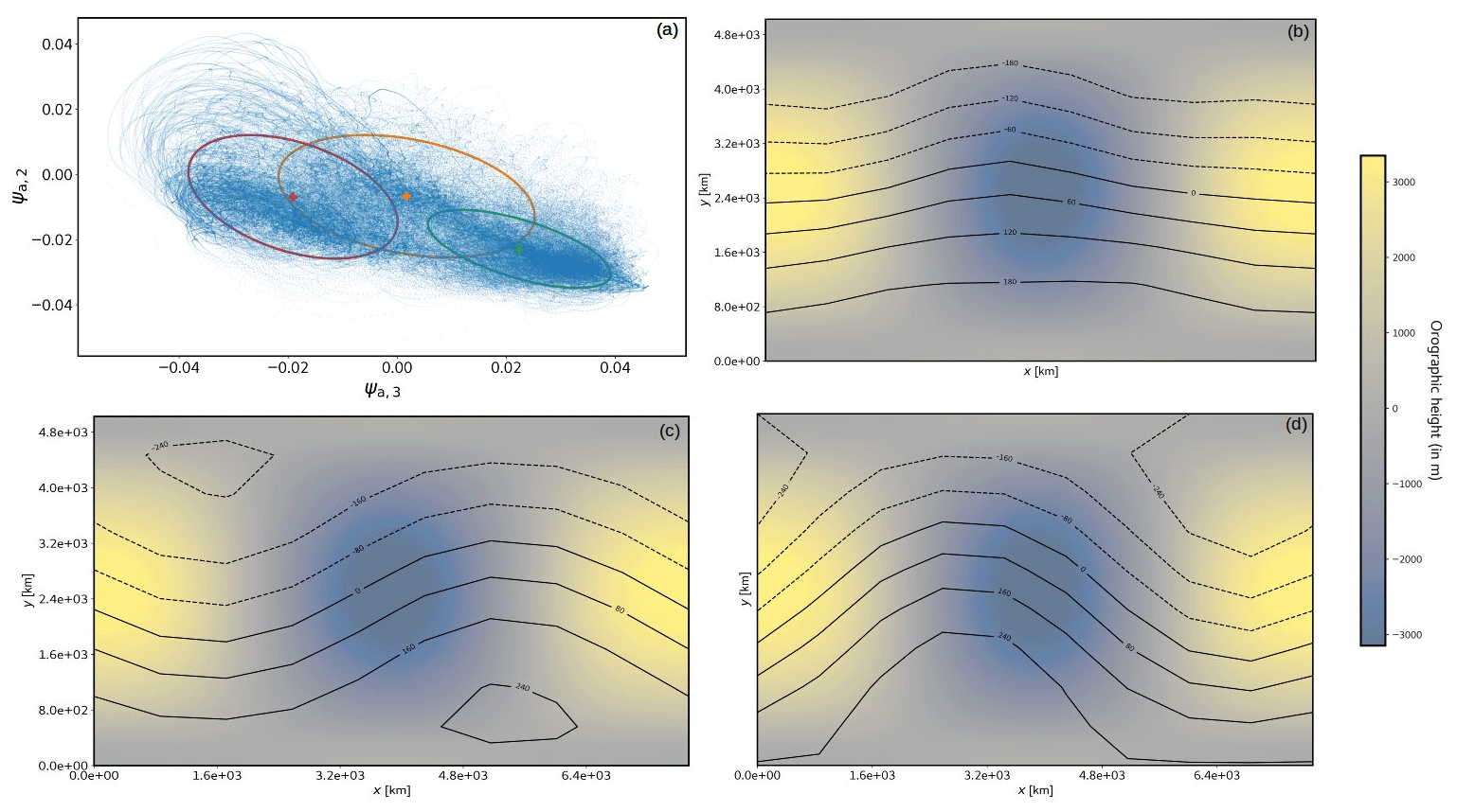
Figure B2 Same as Fig. B1 but for k_d=0.08. Here the red (c) and green clusters (d) are both blocking regimes, and the orange one (b) is a transition regime.

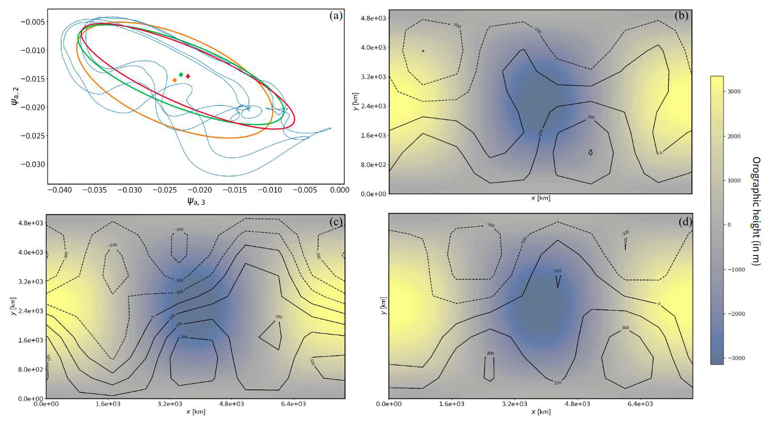
Figure B3 Same as Fig. B1 but for k_d=0.105 where the system exhibits periodic behavior resulting in non-identifiable flow regimes and indistinguishable clusters.

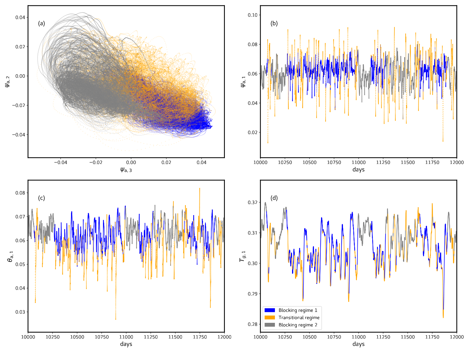
Figure B4 Phase space dynamics of the model projected on the (ψ_a,3, ψ_a,2) plane (a) for k_d=0.08. The figure illustrates the Gaussian mixture clustering results, where each data point is colored according to its corresponding cluster or flow regime. Panels (b), (c), and (d) depict the temporal evolution of the barotropic (ψ_a,1) and baroclinic (θ_a,1) atmospheric streamfunction, along with ground temperature (T_g,1) for C_g=300 Wm⁻² and k_d=0.08, with colors corresponding to their respective clusters.