the Creative Commons Attribution 4.0 License.
the Creative Commons Attribution 4.0 License.
 | 21 May 2024
Classification of synoptic circulation patterns with a two-stage clustering algorithm using the modified structural similarity index metric (SSIM)
Kristina Winderlich
Clementine Dalelane
Andreas Walter
We develop a new classification method for synoptic circulation patterns with the aim to extend the evaluation routine for climate simulations. This classification is applicable to any region of the globe of any size given the reference data. Its unique novelty is the use of the modified structural similarity index metric (SSIM) instead of traditional distance metrics for cluster building. This classification method combines two classical clustering algorithms used iteratively, hierarchical agglomerative clustering (HAC) and k-medoids, with only one pre-set parameter – the threshold on the similarity between two synoptic patterns expressed as the structural similarity index measure (SSIM). This threshold is set by the user to imitate the human perception of the similarity between two images (similar structure, luminance, and contrast), whereby the number of final classes is defined automatically.
We apply the SSIM-based classification method to the geopotential height at the pressure level of 500 hPa from the ERA-Interim reanalysis data for 1979–2018 and demonstrate that the built classes are (1) consistent with the changes in the input parameter, (2) well-separated, (3) spatially stable, (4) temporally stable, and (5) physically meaningful.
We demonstrate an exemplary application of the synoptic circulation classes obtained with the new classification method for evaluating Coupled Model Intercomparison Project Phase 6 (CMIP6) historical climate simulations and an alternative reanalysis (for comparison purposes): output fields of CMIP6 simulations (and of the alternative reanalysis) are assigned to the classes and the Jensen–Shannon distance is computed for the match in frequency, transition, and duration probabilities of these classes. We propose using this distance metric to supplement a set of commonly used metrics for model evaluation.
Please read the corrigendum first before continuing.
-
Notice on corrigendum
The requested paper has a corresponding corrigendum published. Please read the corrigendum first before downloading the article.
-
Article
(1919 KB)
- Corrigendum
-
Supplement
(3192 KB)
-
The requested paper has a corresponding corrigendum published. Please read the corrigendum first before downloading the article.
- Article
(1919 KB) - Full-text XML
- Corrigendum
-
Supplement
(3192 KB) - BibTeX
- EndNote


Research institutions around the world conduct climate studies and share their knowledge with society and policy makers through the Intergovernmental Panel on Climate Change (IPCC, https://www.ipcc.ch, last access: 7 May 2024). The climate simulations used in the IPCC reports are available to other scientists, besides those who run the models, through the Coupled Model Intercomparison Project (CMIP, https://www.wcrp-climate.org/wgcm-cmip, last access: 7 May 2024). The first two phases (CMIP1 and CMIP2) of this initiative addressed the ability of numerical climate models to simulate the present climate and to respond to an increase in carbon dioxide concentration in the atmosphere (Meehl et al., 1997, 2000). The extended follow-up phase CMIP3 (Meehl et al., 2007) provided output of coupled ocean–atmosphere model simulations of 20th–22nd century climate for the 4th Assessment Report (AR4) of the IPCC (https://www.ipcc.ch/report/ar4/syr/, last access: 7 May 2024). As the number of climate simulations in the subsequent projects CMIP5 (Taylor et al., 2012) and CMIP6 (Eyring et al., 2016) continued to increase, new requirements for the “quality” and “reliability” of such simulations emerged. Having multiple models at their disposition, final users have a choice to use all models or only models which pass a quality check, i.e. an evaluation routine. Although testing and comparing models may create an illusion of finding the best one in all its features, we emphasize here that there is no universally valid and absolutely objective evaluation procedure for all purposes. It is important to include a broad suite of metrics in the evaluation spectrum, but various applications may require different subsets of these metrics.
Hannachi et al. (2017) emphasized the importance of the correct representation of weather regimes, their spatial patterns, and persistence properties in global circulation models as they could properly simulate the climate variability and long-term climatic changes under an external forcing such as, for example, the global warming. However, traditional techniques for climate model evaluation, which are rooted in evaluation techniques for numerical weather prediction models, mainly focus on individual variables and derived indices as summarized by Gleckler et al. (2008). These techniques use scalar variables, called “metrics”, and often illustrate symptoms of problems without explaining their causes that may originate from incorrect simulation of synoptic weather. As some studies have already demonstrated that the performance of a model varies as a function of weather type (Díaz-Esteban et al., 2020; Nigro et al., 2011; Perez et al., 2014; Radiæ and Clarke, 2011) we suggest accounting for model synoptic behaviour in evaluation routines. But how can we capture the correctness of the large-scale atmospheric dynamics in models?
The atmospheric circulation is a continuum that gradually changes and its dynamics can be described by a finite number of representative “states” or “typical patterns”, i.e. classes. Hochman et al. (2021) showed that such representation of the atmosphere by quasi-stationary circulation patterns, often also termed weather regimes, is a physically meaningful way to describe the atmosphere (and not only a useful statistical categorization as it may be argued). Muñoz et al. (2017) also suggested using the weather-typing approach to diagnose a range of variables in a physically consistent way, helping to understand causes of model biases. For evaluation purposes, any climate model simulation can be represented as a sequence of typical synoptic situations that are previously classified. Common variables used for representing the synoptic circulation are sea level pressure, geopotential heights, and wind vector fields. Statistical measures, such as frequency and duration of each class, computed from the assigned sequence can be evaluated against reference data derived, for example, from a reanalysis.
Many questions arise when building a classification of weather situations.
-
On which spatial and temporal scales should weather situations be classified?
-
Do the frequency and persistence of each weather situation play a role in the classification?
-
How many classes are sufficient to describe the atmospheric circulation?
Answers to these questions are not trivial and strongly depend on the purpose of the classification.
Weather patterns can be defined at a regular temporal step, typically 1 d (Lamb, 1972; Hess and Brezowsky, 1952; Fabiano et al., 2020; Cannon, 2012), and classified independent of their duration (James, 2006; Cannon, 2012; Beck et al., 2007; Fettweis et al., 2010). Alternatively, only recurrent, quasi-stationary, and temporally persistent states of the atmospheric circulation would be classified (Dorrington and Strommen, 2020; Hochman et al., 2021), eliminating short-term patterns in the final set of classes.
There is no “universally correct” recipe for how to build synoptic classes and how many of them. Each application requires a number of classes constructed in a way best suited for its purposes. A set of classes can be determined subjectively by an expert, such as the well-known Hess–Brezowski Grosswetterlagen (Gerstengarbe and Werner, 1993; James, 2006; Hess and Brezowsky, 1952) or the Lamb weather types (Lamb, 1972), or using an automated classification method. Multiple different synoptic classifications have been developed over years as summarized by Yarnal et al. (2001) and Huth et al. (2008). An overview and systematization of existing classification methods for synoptic patterns were compiled in a joint effort of multiple European institutions in the COST Action 733 and summarized in the final project report (Tveito et al., 2016). A large number of classes is often used in classification methods rooted in synoptic meteorology. Such methods – for example, the ZAMG classification with 43 classes (Baur, 1948; Lauscher, 1985) and the Grosswetterlagen-based classification by James (2006) with 58 weather types (29 for winter and 29 for summer) – give priority to a high structural differentiation among synoptic patterns, at the same time trying to maximize the homogeneity inside classes. This attempt may produce some classes which have a small number of members or could even be empty. On the other hand, methods that use a small number of classes focus on large-scale circulation regimes and can be used for investigating possible precursors to their changes, for example shifts of the jet stream (Dorrington and Strommen, 2020). These methods may handle the pattern diversity in a suboptimal way: prioritize a low number of classes over the high intra-class homogeneity and leave multiple synoptic patterns unclassified.
Our purpose is to extend a traditional evaluation routine for climate models, which typically rests on a set of metrics for scalar variables (Gleckler et al., 2008), by a set of diagnostics considering the correctness of weather pattern representation. We are not the first ones to evaluate model dynamics in such a way. Riediger and Gratzki (2014) evaluated climate indices (mean values or hot, cold, wet, and dry days) computed for five global circulation models and a reanalysis conditioned on different weather types in a recent and a future climate using a threshold-based classification method for the central European region (Dittmann et al., 1995). Cannon (2020) used two atmospheric classifications constructed from two reanalyses for evaluating historical simulations of 15 pairs of global climate models from CMIP5 and CMIP6 datasets; the number of circulation classes used in this study was 16 as suggested in the COST733cat database over smaller European domains (Philipp et al., 2010). Herrera-Lormendez et al. (2021) used the Jenkinson–Collison classification adapted to Europe for evaluating some CMIP6 models against three reanalyses and analysed future changes in circulation for these models.
A “good” set of weather types should be able to describe all physically admissible states and events in the climate system; i.e. rainfall events and heat periods can be explained by an occurrence of individual weather types or a particular sequence of certain weather types. Muñoz et al. (2017) and Nguyen-Le and Yamada (2019) investigated rainfall intensities as a function of weather types. Adams et al. (2020) found that extreme temperature events, as well as cold anomalies, are related to circulation patterns. As we keep in mind the possible linkage between weather types and extreme weather, we would like to have an automated classification that
-
produces structurally differentiated classes (similarly as done in synoptic meteorology),
-
is applicable to any domain on the globe,
-
provides high homogeneity inside classes, and
-
encompasses almost all synoptic situations, leaving no or very few situations unclassified.
In our opinion, the last condition is especially important because rare synoptic situations may be linked to severe weather and should be carefully handled in the evaluation procedure for climate models. Therefore, the wide variety of classification methods that focus on very few quasi-stationary weather regimes do not suite our purpose as they eliminate rare synoptic patterns from the analysis. Semiautomated classifications do not suite our purpose of model evaluation either because these methods require expert knowledge to define weather types in the considered region; this would limit our future options of evaluation to only regions with available expert knowledge.
A relatively new group of synoptic classification methods uses self-organizing maps (Kohonen, 2001). These SOM methods employ a neural network algorithm that discovers patterns in data in an unsupervised way. Such algorithms have an advantage compared to methods based on the principal component analysis (PCA) and subsequent clustering of data as SOMs do not require orthogonality and stationarity of identified classes. Studies that use the SOM technique to classify synoptic patterns and relate these patterns to local weather (Cassano et al., 2006; Gervais et al., 2016; Hewitson and Crane, 2002; Jiang et al., 2011) typically use a pre-defined number of classes and employ the Euclidean distance measure for similarity between data elements and centroids for representing cluster centres. Also, the majority of classification methods included in the COST733cat database (Philipp et al., 2010) and in the literature (Cannon et al., 2001; Hochman et al., 2021; Grams et al., 2017; Muñoz et al., 2017; Fabiano et al., 2020) use the k-means clustering algorithm (Milligan, 1985) in conjunction with the Euclidean distance as a metric to measure the degree of similarity between clustered data elements. In this paper we elaborate on the drawbacks of using mean fields as cluster centres in the classification of atmospheric data fields and suggest an alternative representation of cluster centres.
Distance metrics typically used in classification algorithms are often Euclidean norms (L2 norms), mean squared error (MSE), or Pearson's distance. MSE remains the standard criterion for comparing modelled and observed signals in climate science and in optimization routines despite its weak performance and serious shortcomings in comparing structured signals (pressure or geopotential fields can also be seen as “images”) as thoroughly discussed by Wang and Bovik (2009). Following the suggestions of Wang and Bovik (2009), we refrain from using MSE as a distance measure in classifying weather types and propose using the alternative structural similarity index metric (SSIM) introduced by Wang et al. (2004) for comparing geopotential fields.
Following the abovementioned arguments, we introduce the new two-stage classification method for synoptic circulation patterns as an alternative to existing methods of clustering. The novel approach allows accounting for rare synoptic situations, which may be linked to severe weather, and builds synoptic classes automatically without prior expert knowledge. This alternative method, in our opinion, bears its own scientific value because as the very least it corroborates previous results, but it even improves upon those previous results in both statistical (number of classes is defined automatically) and climatological aspects (all synoptic situations are classified, applicable to arbitrary regions of the globe without further expert knowledge). The novelty of this method consists of the following features.
-
It classifies all input data without pre-filtering and pre-initialization of classes.
-
It builds classes with strong structural differentiation and high inter-class homogeneity.
-
It uses a structural similarity metric instead of a distance metric for classifying data.
-
It represents classes by their medoids instead of centroids.
-
It uses an iterative combination of the hierarchical agglomerative algorithm with a partitioning k-medoids algorithm to determine the number of clusters automatically.
This classification algorithm does not need an initial distribution of elements and gradually continues building and reviewing clusters until there are no more clusters to be built and reviewed according to a given threshold of similarity.
We demonstrate that the new classification produces a set of well-separated classes, not necessarily of similar size, that are consistent (small changes in the pre-set parameter do not alter classes strongly), stable with respect to the temporal selection of data (for example, randomly chosen and shuffled), stable across various spatial resolutions and data volumes, and physically interpretable (i.e. final classes represent real synoptic situations).
In this paper we describe the new classification method and demonstrate its application to evaluation of global circulation models. The final result of the evaluation is expressed as the Jensen–Shannon distance that can be computed with models statistics.
The paper is structured in the following way: (1) introduction, (2) data and domain description, (3) description of the classification method, (4) presentation of resulting classes, (5) presentation of weather extremes affiliated with the synoptic classes, (6) use of the derived classes in computing the distance metric for evaluating CMIP6 climate simulations, and (7) our conclusions and an outlook for future applications.
We use four datasets in this study.
The first dataset, a dataset of synthetic data, is used to demonstrate the performance of the classification method explaining why modifications to the classical k-means algorithm are necessary. We generated these synthetic data using Gaussian-shaped anomalies trying to mimic the smooth shape of geopotential patterns (the real data we wish to use later) and to illustrate how such anomalies are treated by the classification algorithm. The synthetic data are generated randomly and have no genuine structure of the geopotential patterns. However, any clustering algorithm should produce clusters governed by the position of the largest anomaly in the domain and its sign. The original circular shapes of the synthetic generated data help to illustrate how such shapes are grouped into classes by classifications in a simpler manner as if we would have used the real data for this demonstration (using real data makes these distortions less obvious).
The synthetic data of 1000 elements were generated for the domain of 22×22 grid points. Each field includes one large and 10 smaller Gaussian-shaped superimposed anomalies with randomly chosen sizes that are randomly placed within the domain and with randomly chosen signs (negative or positive anomaly); additionally, a randomly generated linear shift of the mean is added to each field. Examples of generated anomaly fields are shown in Fig. 1.
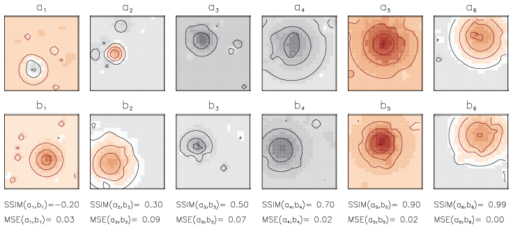
Figure 1Examples of synthetic data fields. Fields are shown pairwise (a1–b1, a2–b2) to demonstrate how visually perceived similarity is quantified in terms of SSIM and MSE given under the lower plot for each pair. Contour lines show the amplitude of negative anomalies (black) and positive anomalies (red) with an interval of 0.25. Pairs are ordered by their SSIM values from a dissimilar pair (on the left) to a strongly similar pair (on the right). Note: smaller MSE does not guarantee larger SSIM values as for the pair a1–b1.
The second dataset, made up of data from the ERA-Interim reanalysis (Dee et al., 2011) for the period of 1979–2018, is used as a realistic historical representation of the atmospheric circulation in Europe. The original spatial resolution of these data is approximately 80 km (T255 spectral) on 60 levels. Simulated synoptic regimes are represented by the geopotential height (zg) at the pressure level of 500 hPa sampled daily at 12:00 UTC for two practical reasons: (1) it often matches the midday peak in extreme weather conditions and (2) it is a typically available time for model output (for subsequent model evaluation). There is no necessity to use more frequent fields, for example 1-, 3-, or 6-hourly, as this would increase the data volume but would not add more information to the synoptic patterns: these patterns do not replace each other in a few hours but extend over large spatial scales and may persist for several days or longer. Data fields zg are sampled on a grid of 2°×3° as suggested by participants of the COST Action 733 (Tveito et al., 2016). The coarse-scale sampling is sufficient due to the fact that the synoptic-scale 500 hPa geopotential height does not require high resolution to reproduce the key physical mechanisms (Muñoz et al., 2017). The chosen domain (Fig. 2) has 22×22 grid points with the lower left corner at 20° W, 29° N.
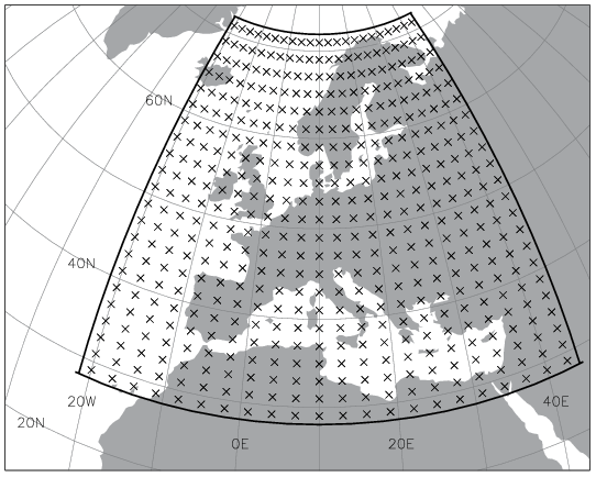
Figure 2Domain for the classification of synoptic circulation patterns: crosses show sample points every 2° in latitude and every 3° in longitude, with 22×22 grid points in total. The solid black line shows the outer edge of the domain.
Some typical synoptic patterns may occur in different seasons but should be grouped into one class. As the mean and the variance of the geopotential change seasonally (larger in summer, smaller in winter) the original data should be pre-processed in order to reduce the sensitivity of the classification to the summer variance and the mean in the data. To allow this, we pre-process the original geopotential height fields (zg) by removing the seasonal amplitude from the original daily data and normalize the resulting fields by the daily standard deviation as in Eq. (1):
The mean and the standard deviation are calculated for each grid point and for each day of the year from the 40 years of reanalysis data; both fields are smoothed in time with a 151 d running average for each grid cell of the domain. The long smoothing period was chosen with the purpose of producing smooth seasonal curves of the mean 500 hPa-geopotential and its standard deviation. Using such smooth mean and standard deviation curves for the normalization of the geopotential fields (prior to clustering), we preserve much of the field's anomaly. The resulting geopotential anomaly fields are used in the classification.
Additionally to zg, we retrieve ERA-Interim daily near-surface atmosphere temperature (tas) and daily total precipitation (pr) to demonstrate potential weather extremes affiliated with each synoptic class (See Sect. 5). For these daily variables we compute 90th percentile map at the original spatial resolution within the chosen domain over the period 1979–2018. For each daily variable we create a map of exceedance: locations where the variable exceeds its 90th percentile get the value of 1; otherwise, the value is 0. These binary maps are summed up for days of the same synoptic class and normalized by the number of days in this class. The final map represents the exceedance probability for the synoptic class.
The third dataset is the alternative reanalysis NCEP1 (Kalnay et al., 1996). Any other reanalysis dataset may be taken. Assuming that the alternative reanalysis captures the synoptic circulation of the reference data from ERA-Interim (both reanalysis products use and share at least some portion of global weather observations) better than any unconstrained global circulation model, the evaluation of an alternative reanalysis gives an estimate of the lower bound for the attainable value of the distance metric.
The fourth dataset is made up of climate model output from the Coupled Model Intercomparison Project Phase 6 (CMIP6, https://wcrp-cmip.org/cmip-data-access/, last access: 7 May 2024) (Eyring et al., 2016). Based on data availability we chose 32 global circulation models for the historical period 1979–2014, preferably simulation version r1i1p1f1 when available or r1i1p1f2/r1i1p1f3 otherwise. We use the output data for geopotential height at 500 hPa for the 32 chosen models to demonstrate a possible evaluation routine that uses the synoptic classes derived from the reference reanalysis.
A frequently used approach for identifying circulation regimes is to apply the k-means clustering algorithm (Milligan, 1985) to the synoptic circulation data: an overview can be found in the COST733cat database (Philipp et al., 2010) and in the recent literature (Cannon et al., 2001; Hochman et al., 2021; Grams et al., 2017; Muñoz et al., 2017; Fabiano et al., 2020). K is the number of classes to be built (this number must be set prior to the classification) and “means” denotes the average of data elements within each class (also called centroid). The k-means method partitions the input data into k clusters so that each data element belongs to the cluster with the nearest centroid, minimizing within-cluster variances; the k-means method is simple and always converges to a solution. Although k-means and its multiple variants, as well as the more general group of SOM-based methods with neighbour radius ≥1, are commonly applied in the field of atmospheric science, they exhibit serious limitations with regard to our aims.
-
Use centroids (means of all elements in a cluster) to represent classes: using mean fields as cluster centres in the classification of atmospheric data fields may be suboptimal and lead to building classes with dissimilar elements (as shown later in this paper).
-
Require a pre-specified number of classes.
-
Use structure-insensitive distance metrics (e.g. Euclidean distance) for the optimization of the element assignment among classes. The k-means clustering assigns every data element to the cluster centre that is closest to it. This makes the method sensitive to noise in the data and may lead to an assignment of a data element to a structurally dissimilar cluster centre (Falkena et al., 2021); a pair of data fields is structurally dissimilar when it shows patterns perceived by an observer (or characterized by any structural similarity measure) as dissimilar.
The mean squared error (MSE) and the Pearson correlation coefficient (PCC) are probably the dominant quantitative performance metrics in the field of model evaluation and optimization. The k-means clustering algorithm typically uses the MSE to measure the distance between clustered data elements. However, Wang and Bovik (2009) demonstrated that the MSE has serious disadvantages when applied to data with temporal and spatial dependencies and to data where the error is sensitive to the original signal. Mo et al. (2014) in turn demonstrated that the PCC as a metric is insensitive to differences in the mean and variance. However, atmospheric data (pressure, geopotential, temperature fields) often reveal dependencies in time and space, as well as shifts in the mean and differing variances. Both studies mentioned above (Mo et al., 2014; Wang and Bovik, 2009) recommend using an alternative measure for signal similarity, the structural similarity index (SSIM), to quantify the goodness of match of two patterns. The SSIM (Wang et al., 2004) simulates the human visual system that “recognizes” structural patterns and error signal dependencies and shows a superior performance as a similarity measure over the MSE and PCC.
3.1 Structural similarity metric (SSIM) and its modification
We use the structural similarity index (SSIM) (Wang et al., 2004) to measure the similarity between synoptic patterns (SP) represented by the geopotential height anomalies . These fields are highly structured images, meaning that the sample points of these images have strong spatial dependencies, and these dependencies carry important information about the structures of the highs and lows in the field. The SSIM incorporates three perception-based components of image difference – structure (covariance), luminance (mean), and contrast (variance):
where x and y are non-negative signals, μx and μy are average values for x and y, σx and σy represent variance for x and y, σxy is the covariance of x and y, and c1 and c2 are stabilizing constants for weak denominator.
For each pair of images the SSIM value is computed, which ranges . The if and only if x=y (x and y are two identical images). In practice, most SSIM values are positive and , identifying some difference between two images. Negative values of SSIM only occur when the covariance term σxy is negative. The SSIM value is usually computed for multiple sliding windows inside the image. But for simplicity here, only one SSIM value is computed for the whole domain. As the selected domain is relatively large and extends to high latitudes, areal weighting was applied to all fields prior to computing SSIM.
From the formulation of SSIM (2) it is important to note that it is applicable as a similarity metric only to same-sign data. However data in climate-related applications are often mixed-sign and/or normalized (with the mean around zero). Therefore, SSIM in its original form (2) cannot be used as the product of means μx and μy with different signs in combination with the negative covariance term σxy as it would yield a positive SSIM value. To overcome this limitation Mo et al. (2014) proposed a “shift” of x and y by the minimum value of the two fields: and are non-negative, where . However, this modification weakens the sensitivity of SSIM to the difference between the means as a result of the enlarged denominator.
We suggest an alternative modification, which only moderately modifies the magnitude of the denominator, preserving the difference between the original means μx and μy:
where
The latter formula (Eq. 3) is applicable to floating-point data with mixed sign.
The choice of stabilizing constants is “somewhat arbitrary” as SSIM is “fairly insensitive” to these values – the authors say (Wang et al., 2004). Baker et al. (2022) suggest that c1 and c2 should be the same to make both terms equally influential and propose that c1 and c2 be “small enough to not disproportionately influence” the final SSIM value. We set as suggested by Baker et al. (2022).
3.2 Examples of MSE and SSIM as measures of similarity
We get the first glance at the ability of SSIM to capture the structural similarity from its application to the synthetic data (Fig. 1). Figure 1 shows fields of the synthetic pairs of maps (ai, bi) for , their respective values of structural similarity SSIM(ai,bi), and the mean square error MSE(ai,bi) under each pair. Assuming MSE and SSIM are capable measures for similarity between two signals we expect MSE to decline with growing SSIM as the distance between more similar signals should be smaller than the distance between less similar signals. We ordered exemplary pairs in Fig. 1 by their increasing SSIM value (from the left to right side of the plot), but we see that respective MSE values of these pairs do not decline monotonously with increasing similarity. It is remarkable that ; i.e. the distance between the pair of signals (a1, b1) is smaller than the distance between the pair (a2, b2), although signals a1 and b1 are obviously less similar to each other (they have anomalies of different sizes and placements) than signals a2 and b2. This example implies that using MSE in a clustering algorithm would rather group the pair (a1, b1) into the same class as the pair (a2, b2). Such preference results from the insensitivity of MSE to the spatial correlation and could lead to building classes with structurally dissimilar members. Using SSIM instead of MSE helps to capture the degree of similarity between clustered signals in a better way for the exemplary synthetic data.
Now we show that SSIM applied to real geopotential height anomalies is preferable over MSE: in Fig. 3 both pairs of geopotential anomalies have ; however, the pair a−b has a high value of , whereas for the other pair indicates dissimilarity. In other words, the MSE does not detect “obviously” dissimilar geopotential anomaly patterns.
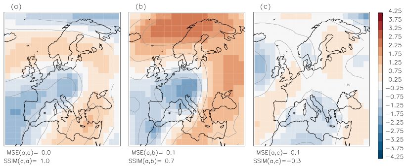
Figure 3The pairs of geopotential anomaly fields a–b and a–c have the same small MSE=0.1 but are strongly different in terms of SSIM: means that fields a and b are similar, and means that fields a and c are dissimilar. Contour lines show the amplitude of anomalies with an interval of 1.
These two examples, with the synthetic data (Fig. 1) and the real geopotential data (Fig. 3), illustrate the weakness of the MSE as a similarity metric for comparison (and subsequent clustering) of structured data fields compared to the SSIM. Therefore, we propose using SSIM as a similarity measure in a new clustering algorithm.
3.3 Modifications of k-means applied to synthetic data
To support our previous arguments (about deficiencies of MSE distance measure) we set up and run three experimental classifications on the synthetic data: (1) the classical k-means clustering algorithm with the distance measure MSE (k-means-MSE), (2) the k-means with the alternative similarity measure SSIM (k-means-SSIM), and (3) the k-medoids with the similarity measure SSIM (k-medoids-SSIM). To obtain comparable results, we initialize all three experimental classifications with the same nine class centres (Fig. 4a), which we a priori derived by an independent run of the hierarchical agglomeration clustering (HAC) algorithm (with the SSIM measure for cluster merging) on the synthetic dataset. The HAC algorithm belongs to a family of hierarchical algorithms and uses a completely different strategy for cluster building as opposed to the partitioning algorithms k-means and k-medoids. This ensures that the classes obtained with HAC for the subsequent initialization of the k-means and k-medoids algorithms do not provide any hidden advantage for either of these algorithms.
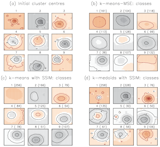
Figure 4Cluster centres: (a) derived by the HAC algorithm and used for the subsequent initialization of the partitioning algorithms; resulting from (b) k-means-MSE classification, (c) k-means-SSIM classification, and (d) k-medoids-SSIM classification. Contour lines show the amplitude of negative (black) and positive anomalies (red) with an interval of 0.25. In panels (b), (c), and (d) above each plot numbers of elements (in brackets) in each class are shown.
Results of k-means-MSE classification (Fig. 4b). These class centres (centroids) visibly deviate from the corresponding initialization fields (Fig. 4a) by the reduced magnitude of anomalies as a result of averaging multiple fields. Classes 3, 5, and 9 also have skewed shapes of anomalies, originally circular, as a result of averaging multiple patterns with variously placed anomalies. We already showed (Figs. 1 and 3) that small MSE does not guarantee the structural similarity of compared patterns. Classes built with k-means-MSE show very little structural detail as a result of building cluster centroids over multiple class elements, whose structural similarity remained unaccounted. The danger of having such classes “with vanishing structure” is that they may serve as attractors for further elements as the clustering algorithm runs trying to minimize MSE only. This leads to the so-called “snowballing” effect; i.e. the more elements are assigned to this class, the less structure its centroid shows, the more elements are assigned, and so on. Cluster 9 (Fig. S1 in the Supplement) is a good example of such a “snowball” class: although all shown elements have comparably small MSE to the final class centre, their visual (for an observer) and computed similarity (value of SSIM) differs strongly as shown for a group of the first 28 elements (out of 132), indicating a strong structural inhomogeneity of patterns contained in one class. This example demonstrates the danger of building snowball classes when using MSE as a distance metric for data with highly structured patterns.
Results of k-means-SSIM classification (Fig. 4c). In an attempt to avoid building structurally inhomogeneous clusters we replaced the Euclidean distance metric MSE by the structural similarity measure SSIM in the classification algorithm, yielding the k-means-SSIM classification. Retrieved classes show some structural patterns that resemble the initial anomaly patterns in the data, although they are weakly pronounced: the amplitude of the large anomaly is reduced and smaller anomalies have nearly vanished by averaging. We see that using SSIM instead of MSE helped to preserve circular shapes of the initial anomalies to some degree, implying that only structurally similar patterns are grouped into one class. However, resulting classes are too smooth in structure (reduced amplitude of anomalies) due to averaging by building centroids.
Assuming the synthetic data represent some physically meaningful field, for example a pressure or a geopotential field, the weakening of the anomaly amplitude by k-means-SSIM and k-means-MSE may have serious implications for the interpretability of the resulting classes; i.e. these classes do not represent any of the original data elements and therefore none of the realistic states of the atmosphere associated with these data. Additionally, such smooth fields would not be able to represent synoptic situations with extreme gradients that may be linked to extreme weather.
We construct a new k-medoids-SSIM classification (Fig. 4d) as we keep the similarity metric SSIM (it showed advantages in structure-preserving compared to MSE) but replace the representation of cluster centres in the clustering algorithm with single “representative” elements – medoids (Kaufman and Rousseeuw, 1990). A medoid is the element of the class with the smallest dissimilarity to all other elements in this class. Each medoid itself is part of the data. Retrieved classes (Fig. 4d) show strong anomaly amplitudes and do not necessarily resemble their initialization fields, except classes 2 and 7: those medoids remained nearly “untouched” by the classification. The distribution of cluster elements in k-medoids-SSIM is done at each step of the algorithm by computing the medoid (the element with most mean similarity to all cluster elements) of each cluster. This procedure is less sensitive to the addition of new elements to the cluster than the recomputation of centroids. New cluster elements do not necessarily modify the cluster's medoid defined at the previous step of the algorithm. This robustness of the k-medoids algorithm (Kaufman and Rousseeuw, 1990) with regard to outliers and noise helps to avoid snowballing in cluster building and explains the match of classes 2 and 7 with their initial fields; i.e. the initialization of these classes was a “good guess” that proved to be robust throughout the k-medoids-SSIM algorithm (note: initial fields ought not to be good guesses and to remain preserved by the algorithm).
Following the arguments resulting from the application of the three classification algorithms to the synthetic data with structured patterns and structured errors, we propose using the k-medoids algorithm with the similarity metric SSIM for classification of the real geopotential data as only this algorithm builds a set of classes that represent data elements and include only structurally similar elements.
3.4 Initialization of classes
There are multiple ways of defining the number of classes for the partitioning algorithm k-medoids (similarly to k-means) ranging from a random guess to the analysis of the data based on principal component analysis (PCA), also known as empirical orthogonal functions (Huth, 2000). Lee and Sheridan (2012) suggested the initialization of the clustering algorithm by selected PCAs. The reason for this statement was the common assumption that the first few modes returned by PCA are physically interpretable and match the underlying signal in the data. However, Fulton and Hegerl (2021) tested this signal-extraction method and demonstrated that it has serious deficiencies when extracting multiple additive synthetic modes (false dipoles instead of monopoles, which may lead to serious misinterpretation of extracted modes). They also found that PCA tends to mix independent spatial regions into single modes. Huth and Beranová (2021) demonstrated that unrotated PCAs (still often used) result in patterns that are rather artefacts of the analysis than true modes of variability. Additionally, methods that apply PCA filtering to input data do not suit our purpose as these methods eliminate rare synoptic patterns from the analysis, taking into account only a few PCAs with the largest eigenvalues and preventing building classes for rare synoptic situations. Guided by the abovementioned ideas, we decided not to use the PCA-based initialization of the clustering algorithm. For the initialization of k-medoids we suggest using another classical clustering algorithm – hierarchical agglomerative clustering (HAC). An example of HAC-retrieved initial classes is described in Sect. 3.3 with the synthetic data: the HAC algorithm builds classes whose centres are used to initialize the subsequent partitioning algorithm. Furthermore, we suggest using a combination of the two clustering algorithms – HAC and k-medoids – interactively; i.e. merge similar clusters at the first step (HAC) and distribute all data elements to the new clusters at the second step. This two-stage algorithm stops when no similar clusters are left to combine. This is the final set of clusters. The centres (medoids) of final clusters give the set of classes. We describe the new two-stage clustering algorithm below.
3.5 New classification method: two-stage clustering algorithm
Following the previous considerations, we made three essential decisions to modify the classic k-means algorithm in order to construct an algorithm better suited (from our perspective) for building classes of synoptic patterns.
-
Decision 1: use an alternative similarity measure
-
Decision 2: use medoids to represent classes
-
Decision 3: use a two-stage algorithm for the stepwise determination of the number of classes
The two-stage clustering algorithm combines two clustering methods – hierarchical agglomerative clustering (HAC) and k-medoids clustering – in such a way that the output from the first is used as input into the second and vice versa. It inherits the strengths of both contributing algorithms.
Initially each data element represents its own cluster. Similarity between each pair of synoptic patterns is computed as a structural similarity index metric (SSIM). The HAC is a very flexible clustering method that can use any distance or (dis)similarity measure as it allows different rules for aggregating data into clusters (Schubert and Rousseeuw, 2021). At each step, HAC determines the number of clusters and their medoids using a threshold on the SSIM value for merging similar elements into one cluster. The merging threshold THmerge is set by the user and intuitively means the minimal human-perceived similarity of a pair of data elements to be merged in one cluster. K-medoids builds clusters (similarly to the widely known method of k-means) using the medoid prototypes and an arbitrary (dis)similarity measure SSIM for cluster elements (D'urso and Massari, 2019; Schubert and Rousseeuw, 2021): it rearranges all data elements among medoid prototypes (an operation that HAC cannot do) in order to maximize the within-cluster homogeneity. K-medoids in few iterations produces optimized clusters. The new medoids are computed and initialize the next step of HAC and so on.
At each iteration of the two-stage clustering, the two steps are done in the following way.
- 1.
The first step: HAC (merge clusters)
- 1.1.
Clusters with sufficient similarity SSIM > THmerge are merged: clusters with higher similarity are merged prior to those with lower similarity (the similarity between two clusters is measured as the similarity between their medoid fields).
- 1.2.
Temporary cluster medoids are recomputed.
- 2.
The second step: k-medoids (recompose clusters)
- 2.1.
Temporary cluster medoids from the first step are used to initialize the k-medoids clustering algorithm.
- 2.2.
Each data element is assigned to the cluster with the most similar medoid.
- 2.3.
Cluster medoids are recomputed.
- 2.4.
K-medoids clustering is repeated until an optimum (for the given number of medoids) distribution of all data elements is achieved.
Both steps are repeated until there is no sufficiently similar pair of clusters left to be merged.
The presented classification method, as any other classification method, requires some pre-set parameters. The final number of clusters produced by the two-stage clustering algorithm depends on the threshold THmerge for merging elements into clusters and, eventually, on the amount of data to be clustered. Although the choice of THmerge is crucial, there is no statistical or analytical formula for computing this threshold; it can only be chosen subjectively by comparing pairs of synoptic patterns (SPs) and asking observers about their perception of similarity. Examples of “similar” synoptic patterns are shown in Fig. 5. We analysed multiple pairs of SPs and, based on the personal perception of similarity (our own as well as of persons not involved in the development of this classification method), estimated that the threshold value THmerge must lie between 0.40 and 0.45 for recognizable similarity; i.e. pairs with an SSIM value less than 0.40 are generally perceived as dissimilar. Figure 5 illustrates examples of similarity between three exemplary reference SPs and arbitrarily chosen SPs with SSIM values of 0.60, 0.50, 0.45, 0.40, and −0.10 to each reference. SPs with SSIM≥0.60 are “strongly similar” to the reference, SPs with 0.40≤SSIM<0.60 are similar, and those with SSIM<0.40 are “weakly similar” to the reference. SPs with SSIM<0 are “dissimilar” to the reference as, by definition of SSIM, the negative values of SSIM result from negative covariance of compared patterns.
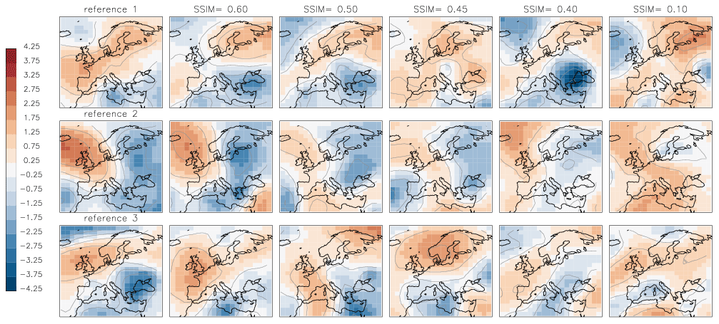
Figure 5Examples of three synoptic patterns (left column – reference). Each row contains examples of alternative synoptic patterns with the SSIM value to the reference. Contour lines show the amplitude of anomalies with an interval of 1.
The definition of the threshold THmerge implies that a reduction of its value loosens the requirement on data similarity for cluster building and provides a smaller number of final classes. On the contrary, an increase in THmerge tightens the requirement on the data similarity for cluster building and therefore leads to a larger number of final classes. At the same time, the higher THmerge also loosens the requirement of separation between classes and permits a higher similarity among them. Thus, varying the value of THmerge may be used, to some extent, to steer the clustering algorithm to produce the number of final classes of a particularly desired magnitude.
Keeping in mind the intended application (evaluation of climate models), the following question arises: how many classes do we need to describe the synoptic flow? In the present study, we use 40 years of daily synoptic patterns and 14 600 daily data fields, which is a usual number of available reference data in climate research for the industrial time. How many classes do we need to represent synoptic situations of these 40 years? Would 10 or 100 be sufficient? The answer to this question is not trivial. The number of derived classes depends on the pre-set parameter THmerge. Because values of THmerge smaller than 0.40 were mainly discarded by observers, testing higher values remains reasonable. We test three values for the threshold THmerge – 0.40, 0.425, and 0.45. Thus, we produce three sets of classes whose separability as a function of THmerge can be analysed.
3.6 Criteria for the evaluation of the clustering algorithm and the choice of the threshold THmerge for class merging
We analyse the performance of the new method using four criteria suggested by Huth (1996): the clusters should (i) be consistent when pre-set parameters are changed, (ii) be well-separated both from each other and from the entire dataset, (iii) be stable in space and time, and (iv) reproduce realistic synoptic patterns.
Cluster consistency. The consistent evolution of classes implies that small changes in the pre-set parameter THmerge lead only to small changes in the classes. To illustrate the sensitivity of the clustering algorithm to the choice of THmerge it was run for three values chosen in the previous chapter: the reference value of 0.40 and two higher values of 0.425 and 0.45. Classes are consistent if an increase in the number of classes caused by a change in THmerge is realized predominantly by splitting a few classes, with others remaining almost unchanged. Such evolution is difficult to quantify. The consistency of the clusters is illustrated by similarity diagrams – diagrams that resemble the “arrow diagrams” in Huth (1996) – for the sets of classes built with the varying parameter THmerge.
Cluster separability. We calculate two metrics introduced in the COST Action 733 report (Tveito et al., 2016) to characterize the separability and within-class variability. Additionally we introduce a new indicator of class separability in terms of similarity. The separation of clusters from randomly chosen data is addressed by the comparison of the metrics or indicators calculated from the clusters to the metrics calculated from “random groups”. The random groups are generated for each cluster as groups of the same size but of randomly chosen data elements (one realization).
Metric 1: the explained variation EV of the data is determined as the residual between 1.0 and the ratio of the sum of squares within classes (synoptic types) WSS to the total sum of squares TSS:
Metric 2: the distance ratio DRATIO is the ratio of the mean distance between elements assigned to the same class DI and the mean distance between elements assigned to different classes DO. The Euclidean distance is used to compute DI and DO:
We construct a new indicator SSIMRATIO for the class separability; similarly to the DRATIO, it is defined as the ratio of the mean similarity within classes (SSIMin) to the mean similarity among different classes (SSIMout):
The mean similarity within classes SSIMin is calculated as the mean “internal” similarity of all classes, where the mean similarity value of each element j to each element k of the same class i is computed.
Here, n is the number of classes, mi is the number of elements in class i, and SSIM(j, k) is the similarity of element j to element k of the same class i.
Mean similarity to other classes SSIMout is calculated as the mean similarity of all class elements to all class elements of all other classes except its own:
where n is the number of classes, mi is the number of elements in class i, SSIM(j, k) is the similarity of element j to element k of any other class but not of the same class, and is the number of all elements in all classes except class j.
Indicator SSIMRATIO could be viewed as an indicator of separability of classes in terms of pairwise similarity value: larger values tell us about stronger within-class similarity in comparison to similarity of other classes.
Note that after comparing the computed metrics and indicators, we discuss the choice of the threshold THmerge. Once chosen, this value of THmerge will be used for further analysis throughout the paper.
According to the stop criterion of the clustering algorithm, each pair of derived classes has a similarity value less than THmerge; i.e. in the classification obtained with THmerge=0.40 pairs of final class medoids are less similar to each other than this threshold. Although the classes are represented by the cluster medoids in the clustering algorithm, it is also reasonable to require that the resulting cluster centroids (means) be at least not strongly similar (SSIM<0.60) to each other. We compute matrices of similarities for medoids and for centroids and analyse how well the medoid separation algorithm provides the separation of centroids in the final set of classes.
Cluster temporal stability. The amount of input of synoptic data is crucial for building the representative set of classes. In periods of only few years of data important synoptic circulations might be simply unrepresented or underrepresented because of long-term variability and therefore missing in the final set of classes. The clustering algorithm is run on a continuously increasing data volume of 1, 2, …, 40 years taken in chronological order: classes for 1979–1979 (1-year period), classes for 1979–1980 (2-year period), and classes for 1979–2018 (40-year period). These input data used in chronological order are called “reference data”.
However, the classification method may produce a different number of classes for data of the same volume but different years. Therefore, in order to produce estimations of class numbers that are robust to the choice of the data, we additionally run 60 classifications for the same data volumes of 1, 2, …, 40 years but picking the data randomly: 30 classifications are built with data sampled randomly out of the whole dataset (bootstrap method for data selection; i.e. data elements may be repeated), and cluster centres are initialized as described above in the method. Clusters with higher similarity are merged prior to those with lower similarity.
A total of 30 other classifications are built on the data selected randomly (but without repetitions) and cluster centres are initialized randomly: cluster pairs are merged randomly without the preference for more similar pairs (also in a case when the input data are the same as the reference data, the random initialization of cluster centres yields different pathways of class merging).
The first group of 30 classifications serves to prove the robustness of the classification method to the selection of the input data. The second group of the 30 classifications serves to illustrate the robustness to the initialization of clusters by the input data. We call both of two groups together “randomized data”.
We expect that after a certain critical data amount is accumulated, further increase does not lead to a discovery of new classes and the temporal stability of the method is achieved. The minimum critical data amount, minNYR (the minimum number of years of data), is set when the number of resulting classes “levels out” and stabilizes.
The total 61 classifications (obtained on 1 reference data + 60 randomized data) are compared to each other in the following way.
-
Search for each class i of the classification k its counterpart (most similar class) j in the classification l: each pair of counterparts (i,j) is detected by maximizing SSIM(i,j) for all i and j.
-
Weight the similarity value SSIM(i, j) by the frequency of i in the classification k: SSIM(i, j)*HIST(i), where HIST(i) is the relative frequency of class i in the classification k.
-
Compute the total mean weighted similarity, mwSSIM, of the classification k to the classification l as the sum of weighted similarity values for all pairs of classes and their counterparts:
where N is the number of classes in the classification k, i=1,N, j is the counterpart of class i (class i belongs to the classification k, class j is belongs to the classification l and is the most similar element to i), and HIST(i) is the frequency of class i in the classification k.
We compute the matrix of mwSSIM values using the 61 classifications retrieved for at least minNYR years of data (note: the number minNYR is defined based on the reference data as the minimum number of years of input data necessary to possibly represent all classes; i.e. a further increase in this number does not increase the number of resulting classes). We require this matrix to have all elements mwSSIM; i.e. all pairs of classifications derived from the same volume of data must be on average similar to each other. This “mean similarity” of the classifications indicates the temporal stability of the classes.
Cluster spatial stability. The stability of the method in space cannot be addressed by applying the clustering algorithm straightforwardly to the data at a lower or higher spatial resolution because the pre-set threshold for cluster merging THmerge is not directly transferable to other spatial grids. The reason for this is simple: a pair of images at a high resolution that appears dissimilar to an observer may have similar low-resolution prototypes (when similarity-determining details are averaged out). However, it can be required that the method determines structurally similar classes at any spatial resolution. To test this, the clustering algorithm is run on the same data but with reduced (4°×6°) and increased (1°×1.5°) spatial resolution. The corresponding datasets were built by resampling the original data at low resolution (4°×6°) and high resolution (1°×1.5°). The retrieved classes from these datasets are compared to the classes on the reference grid (2°×3°).
Cluster reproduction and representativity. The method uses medoids as cluster centres, and therefore the resulting class representatives (set of medoids) are elements of the original data and are physically interpretable and plausible synoptic patterns. However, it is necessary to demand that a cluster medoid represents all cluster elements and their whole entity as a group. For each cluster, we compare the cluster centre (medoid) to the cluster mean (centroid) and calculate their similarity value. Based on the similarity values we analyse the representativity of the cluster elements by the medoids. We require that all medoids are strongly similar (SSIM >0.60) to their centroids. Representing a cluster by a medoid guarantees that the medoid has a minimum similarity to each of the cluster elements; furthermore, it is the element with the largest total similarity to all of cluster elements. If a centroid and a medoid of some class are dissimilar, this indicates that there is a group of elements in the class that is dissimilar to the medoid.
3.7 Statistics for model evaluation and the Jensen–Shannon distance metric
The classification done on the reference data (ERA-Interim reanalysis 1979–2018) yields the set of “reference SP classes”. Each data element of the reference data, of an alternative reanalysis data (NCEP1), and of each CMIP6 model is assigned to one of the reference SP classes to which it has the maximal similarity. We suggest comparing different datasets assigned to the reference SP classes using the following statistics: histogram of frequencies (HIST) for SP classes through all years and seasons, histograms of frequencies for each season (HISTDJF, HISTMAM, HISTJJA, HISTSON), the matrix of transitions (TRANSIT) between available classes (frequency for each SP class to follow another SP class), and probability of persistence (PERSIST) of each SP class for 1, 2, and 25 d. Whereas statistics HIST, HISTDJF, HISTMAM, HISTJJA, and HISTSON are one-dimensional vectors with the number of components equal to the number of SP classes, the TRANSIT and PERSIST are two-dimensional matrices. In the case of high dimensionality, i.e. many SP classes, the comparison of these vectors and matrices may become awkward and ambiguous. Therefore, to quantify differences between pairs of such statistics we suggest weighting contributions of each class by its frequency. We compute Jensen–Shannon divergence (Eq. 14, similar to the widely used Kullback–Leibler divergence but symmetric, and it always has a finite value): frequent elements govern contributions to the distance measure, and rare elements make smaller contributions. The Jensen–Shannon divergence, JSD, used here to measure the similarity between two probability distributions P and Q defined on the same probability space χ, is computed in this way:
where the probability distributions P and Q are the normalized (the sum of all elements is 1.0) frequency histograms as well as transition and persistence matrices of the reference (Q) and a model (P); space χ is a one- or two-dimensional space; and M is the mean probability distribution.
It is common to compute the square root of JSD as a true metric for distance, the Jensen–Shannon distance (Eq. 16):
Such a distance measure is robust against the “noise” from rare classes as well as rare class-to-class transitions but not insensitive to them. We show the Jensen–Shannon distance metric for various pairs of distributions in Fig. S2 and discuss its sensitivity in the Supplement section “Sensitivity of the Jensen–Shannon distance metric”.
4.1 Synoptic classes, effect of the threshold THmerge on the number of classes
We run the classification algorithm on the reference data for a consistently increasing data volume of 1, 2, and 40 years and perform 60 additional runs with the randomized data for the same data volumes. We repeat every run three times, varying the threshold THmerge – the threshold on similarity between two SPs that defines when these SPs are merged into one class. In total runs of the classification algorithm, each yielding a set of classes, are available for the analysis. Figure 6 shows the evolution of the number of classes as a function of the volume of input data for three values of THmerge. Figure 6 illustrates the influence of tightening the requirement on similarity for building clusters: higher thresholds THmerge produce larger numbers of final classes with higher within-class similarity of members. However, at the same time the higher THmerge also loosens the requirement for separation among classes (higher similarity between classes is possible).
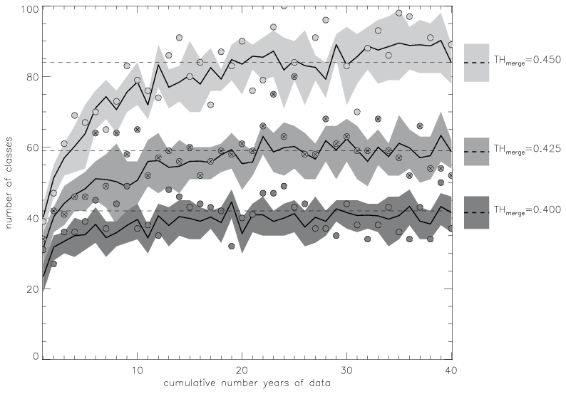
Figure 6The number of classes depends on the threshold THmerge and on the amount of clustered data. For each tested value of THmerge the solid black line shows the mean number of classes computed from 61 classifications (1 with reference data + 60 with randomized data); the shaded area shows the range of 1 standard deviation from the mean. The circles show numbers of classes from classifications with the reference data, and circles with crosses highlight class numbers with THmerge=0.425. The horizontal dashed lines show the mean number of classes for each THmerge value computed from the reference data of 40 years.
The application of three values for the threshold (THmerge=0.40, 0.425, and 0.45) to the reference data with a maximal volume of 40 years produces 37, 52, and 89 classes, respectively. Computed for all 61 classifications (1 with reference data + 60 with randomized data) for varying THmerge the numbers of classes (mean ± standard deviation) are estimated as 42±6, 59±4, and 84±5, respectively (Fig. 6). As expected, the higher values of THmerge provide larger numbers of classes, although not larger standard deviations of these numbers from their means, as a result of tightening the requirement for within-class similarity.
One of the features of our new two-stage clustering algorithm is that it classifies all synoptic patterns including rare ones. This is the reason for the high number of classes built by this algorithm. Figure 7 shows the 37 classes built on 40 years of reference data with THmerge=0.40: the six most frequent classes SP1, SP3, SP4, SP6, SP15, and SP27 together represent ∼42 % of the input data, and 10 most rare classes (SP11, SP20, SP21, SP23, SP26, SP30, SP31, SP34, SP35, SP37) together represent less than 5 % of the input data.
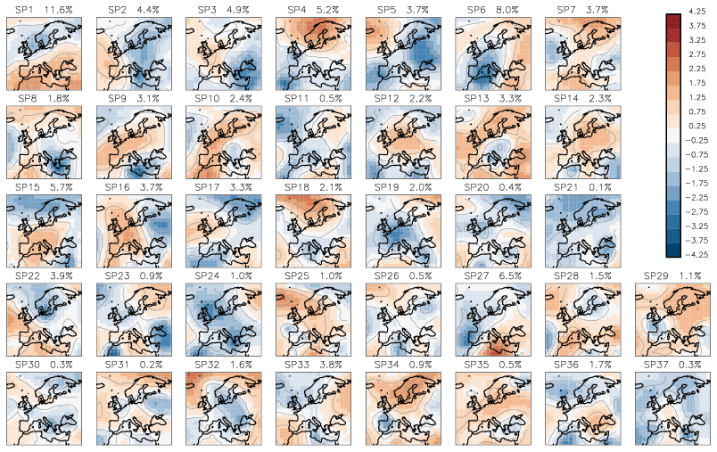
Figure 7SP classes (anomalies of geopotential height) obtained from the reference data (ERA-Interim reanalysis, 1979–2018) with the threshold for similarity THmerge=0.40. Frequencies of SP classes are shown above the corresponding plots.
At first glance all 37 classes in Fig. 7 may look “patchy” and not different enough from each other. However, all these classes are not similar according to our definition as each pair of them has a similarity value smaller than 0.40 (the threshold chosen for the classification algorithm). It is important to note that as the class separation is done in terms of SSIM these classes do not have to be differentiated in terms of MSE. We also show (Figs. 1 and 3) examples of pairs of patterns that are similar in terms of MSE but differ in terms of SSIM.
We take a closer look at the six most frequent SP classes and their full fields (mean + anomaly), as shown in Fig. 8. We compare these six classes to the 29 synoptic weather patterns GWL-REA v1.3 (personal communication) developed at the German Meteorological Service for the Hess–Brezowksy Grosswetterlagen identified in reanalysis data based on correlations in combination with Lamb weather type statistics (James and Ostermöller, 2022). For each of the six SP classes we compare the similarity value to each of the GWL-REA v1.3 fields (geopotential) and identify the most similar one (or pair).
-
SP1: cyclonic southwesterly (SWZ – Südwestlage zyklonal)/cyclonic westerly (WZ – Westlage zyklonal)
-
SP6: low over central Europe (TM – Tief Mitteleuropa)
-
SP27: low over the British Isles (TB – Tief Britische Inseln)
-
SP15: anticyclonic westerly (WA – Westlage antizyklonal)
-
SP4: anticyclonic southeasterly (SEA – Südostlage antizyklonal)
-
SP3: anticyclonic northwesterly (NWA – Nordwestlage antizyklonal)
Correspondences of the six frequent classes to the patterns GWL-REA v1.3 provide us with evidence that, albeit not tuned to and not required to mimic semi-manual classifications, the new classification method determines not just arbitrary synoptic patterns but meaningful synoptic situations described by experts.
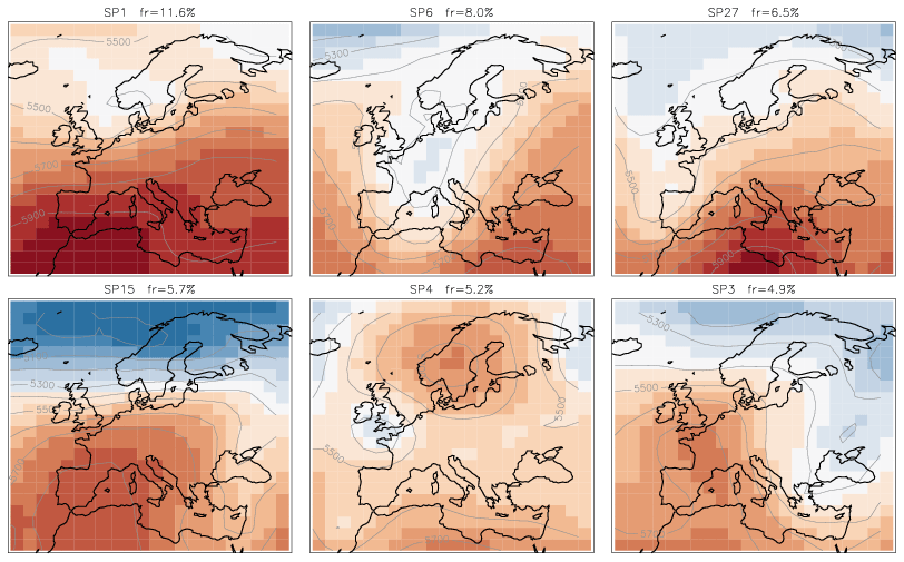
Figure 8Geopotential height (m) for the six most frequent SP classes. The contour lines show the geopotential height levels every 100 m (labelled). The index of each SP class and its frequency are on the top of corresponding plots.
The three sets of classes obtained from the reference data of the full volume with varying THmerge are further analysed with respect to consistency, separability, stability, and representativity of the data.
4.2 Cluster consistency
The evolution of classes built with different values of THmerge is presented in the form of a diagram (Fig. 9), which is also called an arrow diagram, suggesting that lines show how classes are related among different sets of classes. For the arrow diagram in Fig. 9 the classes are derived by running the clustering algorithm on the data for 1 full year. We chose this minimal data volume to build classes with few elements to demonstrate the tightening similarity constraint (by the threshold THmerge) in the best way as classes with large numbers of elements may reveal similarities among subsets of some elements and overload the diagram. In Fig. 9 identical classes (SSIM =1 for the medoids) are connected with thick solid black lines, strongly similar classes () are connected with dashed thick black lines, and similar classes () are connected by thin grey lines, where connections with are dashed. When increasing the merging threshold of 0.40 to 0.425, the total number of classes rises from 31 to 34, with 26 classes remaining identical or strongly similar, 5 classes remaining without a strongly similar counterpart, and 8 new classes emerging. Further increasing the threshold value from 0.425 to 0.45 leads to building 39 classes, with 36 classes remaining identical or strongly similar, 2 classes remaining without a strongly similar counterpart, and 7 new classes emerging. The new emerging classes may have similarity to more than one previous class. We see that 23 classes retain their medoids through the two steps of tightening the similarity constraint (). It is important to note that the identical classes have only one counterpart in each set of classes, which means they are “transferred” to the next set of classes obtained with a higher THmerge and not “split” into new classes. The strongly similar classes typically have only one or – rarely – only a few counterparts; i.e. they are rarely split. New emerging classes may have similarities to multiple original classes. The fulfilment of the demand for the consistency of class evolution is shown by the prevalence of identical classes in the diagram, indicating one-to-one correspondence between classes of different sets. The identical classes, which remain unchanged, are connected with thick solid lines and are often accompanied by a “bunch” of thin lines. Such bunches are mainly produced by the breaking off of some elements from the class on the left side into another class on the right side; the medoid of the original class on the left side remains preserved. For new emerging classes (on the right side) similarities to multiple original classes (on the left side) are acceptable as new classes may contain elements broken off from multiple original left-side classes. An unwanted form of the diagram would be a distribution of classes from set to set connected with thin lines, without clearly preserved identical types.
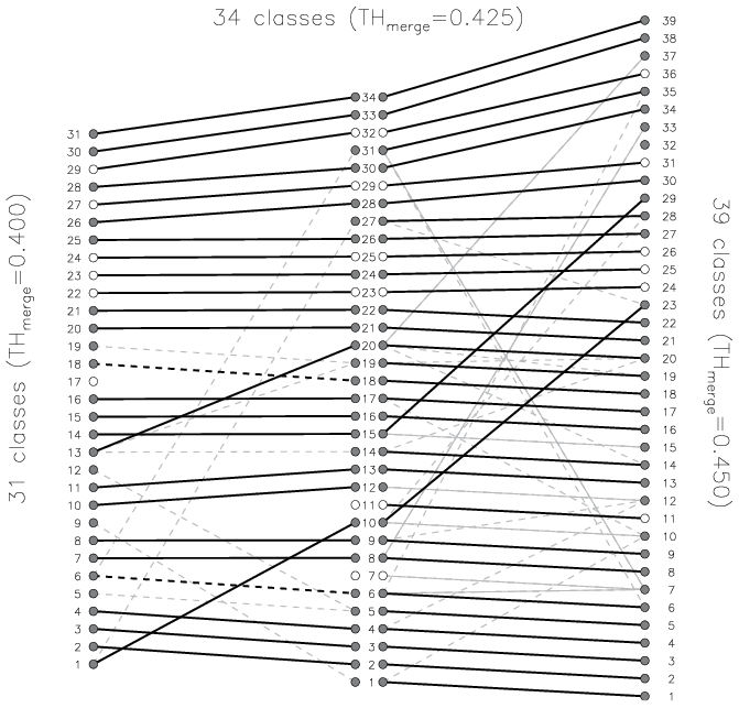
Figure 9Similarity between classes derived with different merging threshold: (left) 31 classes obtained with THmerge=0.40, (middle) 34 classes with THmerge=0.425, and (right) 39 classes with THmerge=0.45. Thick black lines connect identical classes (SSIM=1), dashed black lines connect strongly similar classes (), and grey lines connect similar classes (), where connections with are dashed. Following the solid black lines from left to right, 23 classes retain their medoids.
4.3 Cluster separability
The metrics EV and DRATIO and the indicators SSIMin, SSIMout, and SSIMRATIO computed from the classes obtained with increasing THmerge illustrate the importance of the choice of this threshold and its influence on the number of derived classes and their separability. Table 1 presents the values of the chosen metrics and indicators. Please note that metrics EV and DRATIO illustrate only the influence of the THmerge on the final set of classes and do not describe the quality of classes as they are computed using the Euclidean distance – a measure that was not optimized by the clustering algorithm. Therefore, EV and DRATIO should not be used to assess the absolute performance of the classification, but the relative performance depending on THmerge.
Classifications with larger numbers of classes achieve a better skill EV than those with fewer classes due to the natural fact that a larger number of classes captures a higher fraction of the variation. The extreme case, when the total variation is explained completely (EV =1), is achieved when the number of classes is equal to the number of data. Therefore, it would be dangerous to favour classifications with larger numbers of classes based on this metric. In the present study, the set of classes obtained with THmerge=0.45 provides the highest ratio of explained variation. Clusters of randomly chosen groups, as expected, show nearly no explained variation at all (see Table 1).
Values of the metric DRATIO <1.0 indicate that, on average, elements within classes have shorter Euclidean distance to each other than to elements of other classes. Smaller values of DRATIO indicate a stronger separation of classes. The highest value of THmerge=0.45 provides the lowest value of DRATIO and therefore shows the best separation of classes in terms of Euclidean distance. In randomly chosen groups the value of DRATIO is close to 1, as also shown in Table 1, because of nearly equal distances between elements of the same class and of different classes.
Table 1Metrics for classes obtained in three experiments with varying merging thresholds (THmerge) applied to the reference data of 40 years. Values after “/” are those computed for random groups.
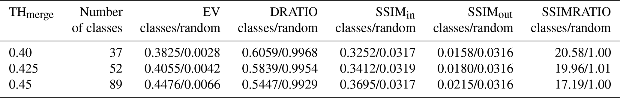
Indicators SSIMin and SSIMout represent the influence of the similarity constraint by THmerge on the separability and homogeneity of the final classes. A good performance of the classification is achieved when similarity among elements of one class SSIMin is much higher than the similarity to elements of other classes SSIMout; i.e. SSIMRATIO should be maximized. The maximal mean similarity among elements of the same class (SSIin=0.3695) is given by THmerge=0.45; however, the mean similarity between pairs of elements of different classes (SSIout=0.0215) is also the highest for this threshold, indicating stronger similarities among elements of different classes as well. Finally, SSIMRATIO – an indicator of class separation in terms of similarity – is highest (20.58) for THmerge=0.40 and shows the favourable separation of classes in terms of similarity among elements.
At this point we make an important decision and choose the classification obtained with the merging threshold of THmerge=0.40 for further analysis for two reasons: (1) this threshold provides good class separation, and (2) using this value we produce fewer classes, which can be meaningfully statistically analysed (a higher threshold value would produce more classes with fewer members). It is also important to note that a smaller number of classes is easier to describe verbally, as well as more intuitive to understand and to separate visually.
The stop criterion in the clustering algorithm guarantees that the maximum similarity between final classes is less than THmerge. In other words, there are no pairs of final medoids similar to each other; otherwise, they would have ended up in the same cluster. Although it cannot be demanded that cluster centroids (means) also satisfy the same criterion for the maximum pairwise similarity, it can be demanded that cluster centroids are at least not strongly similar, i.e. pairwise SSIM<0.60. Figure 10 shows matrices of pairwise similarities for medoids (left) and for corresponding centroids (right). Some pairs of centroids have a similarity value higher than any pair of medoids (circles show SSIM≥0.40) due to the fact that the similarity of medoids but not of centroids was the optimized quantity in the clustering algorithm. The maximal similarity for a pair of centroids is SSIM =0.542 (for centroids 1 and 22); i.e. there is no pair of strongly similar centroids. This gives evidence that the two-stage clustering algorithm that uses medoids as class centres produces classes with meaningfully separated centroids.
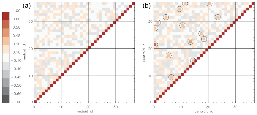
Figure 10Matrix of pairwise similarity values for 37 classes derived with THmerge=0.40. (a) The matrix of SSIM for cluster medoids. (b) The matrix of SSIM for cluster centroids. Circles show similarity values greater than 0.40. Only the upper left half of each matrix is shown due to the symmetry; diagonal elements have SSIM =1.
4.4 Cluster stability
Temporal stability. As we apply the classification algorithm to the data volume of 1, 2, and 40 years. The number of derived classes levels off after approximately 30 years of daily data for all values of THmerge (Fig. 6): this means that all possible synoptic patterns are likely to be captured within 30 years. This data volume matches periods typically used for assessing the variability of other climate variables. Thus, we recommend a minimum critical data amount of minNYR =30 years of data for a temporally stable classification. To support this recommendation, we compute the matrix of the “mean weighted similarity” mwSSIM for 61 sets of classes retrieved for 30, 35 ,and 40 years of data. We require this matrix to have all elements mvSSIM; i.e. pairs of sets of classes must be on average similar to each other.
The number of classes in all 61 sets generated with minNYR =30 years of data varies from 36 to 59 classes, with a mean number of classes of 42. For all 61 sets of classes, we computed the pairwise mean weighted similarity mwSSIM (Fig. 11). The value of mwSSIM(k,l) shows the match of all classes from the set k to all classes from the set l, weighted by the frequency of the classes in the set k. The matrix of pairwise mwSSIM values is not symmetric: as the sets k and l may have different numbers of classes and also the classes differ. When the numbers of classes in sets k and l are different, the following may occur: for class i from set k the class j from set l is the most similar counterpart, but (!) for the class j from the set l a different class h from set k is the most similar one, leaving the class i being the second most similar counterpart for j. In a case of a “perfect match”, the mwSSIM =1, i.e. indicating the identity of two sets of classes. Negative values of mwSSIM would indicate two different sets of classes without any element from one set similar to any element in the other set. In our analysis we only consider mwSSIM for different pairs of classifications (diagonal elements of the mwSSIM matrix are always 1.0 anyway). The maximum mwSSIM (two classifications are almost identical) is attained by 7 % of all pairs, and 54 % of all pairs show strong similarity with mwSSIM ≥0.60. The mean value of pairwise mwSSIM for all (different) classifications is 0.63. Figure 11 shows that all sets of classes are similar to all sets of classes in a pairwise comparison; i.e. all pairwise similarity values are greater than the threshold (THmerge=0.40) with the minimum mwSSIM =0.53. This is indeed a good result. This allows us to say that the two-stage classification produces similar sets of clusters when initialized by randomly chosen subsets of the input data.
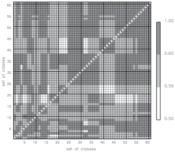
Figure 11Mean weighted similarity, mwSSIM, for each of 61 sets of classes to each other. Each set of classes was derived on minNYR =30 years of input data. The diagonal elements are not shown because mwSSIM =1 of a set of the classes to itself. The matrix is not symmetric: as the sets of classes k and l may have a different number of classes.
We repeat the calculation of mwSSIM for 35 and 40 years of data (not shown) in order to make sure that the classification algorithm produces similar sets of classes for larger data volumes as well. When the data volume is set to minNYR =35 the number of classes varies from 31 to 48 among 61 sets of classes, with minimum mwSSIM =0.55 and mean mwSSIM =0.65. For the maximal data volume (40 years) the number of classes varies from 35 to 49, with minimum mwSSIM =0.54 and mean mwSSIM =0.64. These calculations of mwSSIM with other data volumes only support our previous findings: all pairwise values of mwSSIM are greater than the similarity threshold, indicating that our two-stage clustering algorithm applied to randomly chosen data builds sets of similar classes.
Spatial stability. To test the stability of the method in space, additionally to the classes in the reference dataset (2°×3°), two sets of classes were built at low resolution (4°×6°) and high resolution (1°×1.5°) by resampling the original reanalysis fields to these spatial resolutions. The clustering algorithm was run with the data at each spatial resolution using the same threshold THmerge=0.40. This imposes some restrictions on the interpretation of the results. First, two images at different spatial resolutions derived from the same original image are not necessarily identical in terms of SSIM because they contain different amounts of information. The SSIM value deteriorates with the increasing spatial resolution as the degree of detail in the images grows. Following this argument, it would be impossible to build the same set of classes at various spatial resolutions with the same threshold on similarity. However, it can be required that some classes emerge at all spatial resolutions. Examples of such SP classes are shown in Fig. 12 at three spatial resolutions.
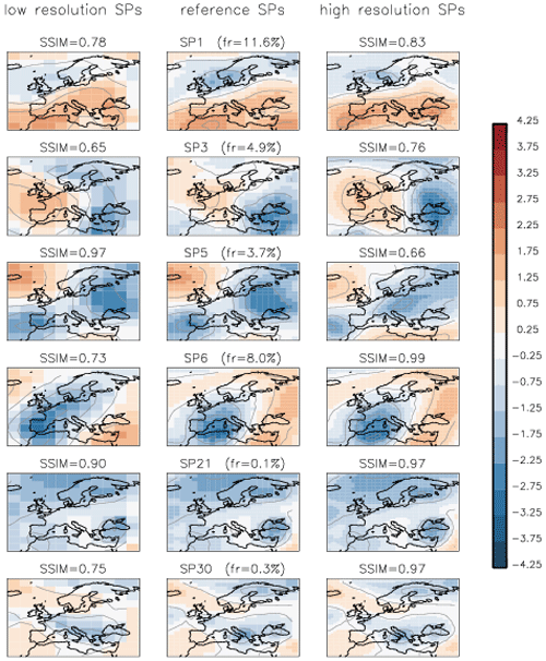
Figure 12Examples of SP classes at three spatial resolutions. The middle column shows reference SPs built from the reference data (2°×3°, 22×22 grid cells) with their frequencies (%). The left-side column shows corresponding patterns at low resolution (4°×6°, 11×11 grid cells) and the right-side column shows high resolution (1°×1.5°, 44×44 grid cells). Both plots for low- and high-resolution counterparts show the SSIM value for the reference SP class on top of each plot.
Figure 12 shows six SP classes at the original resolution (middle plots) and their counterparts in the low- and high-resolution sets of classes. Please note that the SP classes are built at each resolution independently and are not just resampled copies of the same classes. Therefore, some discrepancy must be tolerated among the classes at different resolutions as they are medoids of independently formed classes. Despite such discrepancies the SP classes show essentially the same geopotential anomalies at all spatial resolutions. Although it is not required, classifications based on the three spatial resolutions have 37 classes each. The mean similarity for all 37 SP classes built from the reference data to their counterparts at low resolution is 0.53 and to their counterparts at high resolution is 0.52. These high numbers (>0.40) indicate the ability of the new clustering algorithm to reproduce similar SP classes at different spatial resolutions, i.e. spatial stability of this algorithm.
4.5 Cluster reproduction and representativity
The two-stage classification method uses medoids to represent clusters for reasons of stability. A medoid of a cluster can be seen as “the representative element” of this cluster, i.e. the element most similar to all other elements in the cluster (definition of the medoid). Once the cluster is changed (merged with another one by the hierarchical step for example) the medoids are recomputed. Every new attribution of an element to a cluster is done to the most similar medoid (this ensures exclusive attribution of similar elements to clusters). For the final set of classes we demonstrate that the medoids are strongly similar to cluster means (centroids); i.e. cluster medoids effectively represent the mean patterns of their classes. We analyse the set of 37 classes built from the reference data and compute for each class the similarity value between its centroid and medoid (Table 2). A good representativity is achieved when the medoid and centroid of each class are strongly similar. The Table 2 shows exactly this: SSIM(medoidi,centroidi)≥0.60 for all classes i. If the medoid and the centroid are strongly similar, it guarantees that there are no or negligibly few “extravagantly” dissimilar members in that class. Otherwise, the mean (centroid) would have lost its similarity to the medoid, being distorted by the averaging with dissimilar members. Strong similarity between medoids and centroids for all 37 classes was found, indicating the very good representability of clusters by their medoids. The mean similarity between medoids and centroids over all 37 classes is 0.78 and weighted by the class frequency is 0.79. This is a very good result that shows the strong resemblance between medoids and centroids of the clusters and illustrates the representativity of classes by their medoids.
Table 2Set of 37 SP classes for reference data with THmerge=0.40: index of synoptic pattern (SP), fraction (Fr) in percent of the class in the reference data, and the similarity (SSIM) value between the medoid and centroid of the class.
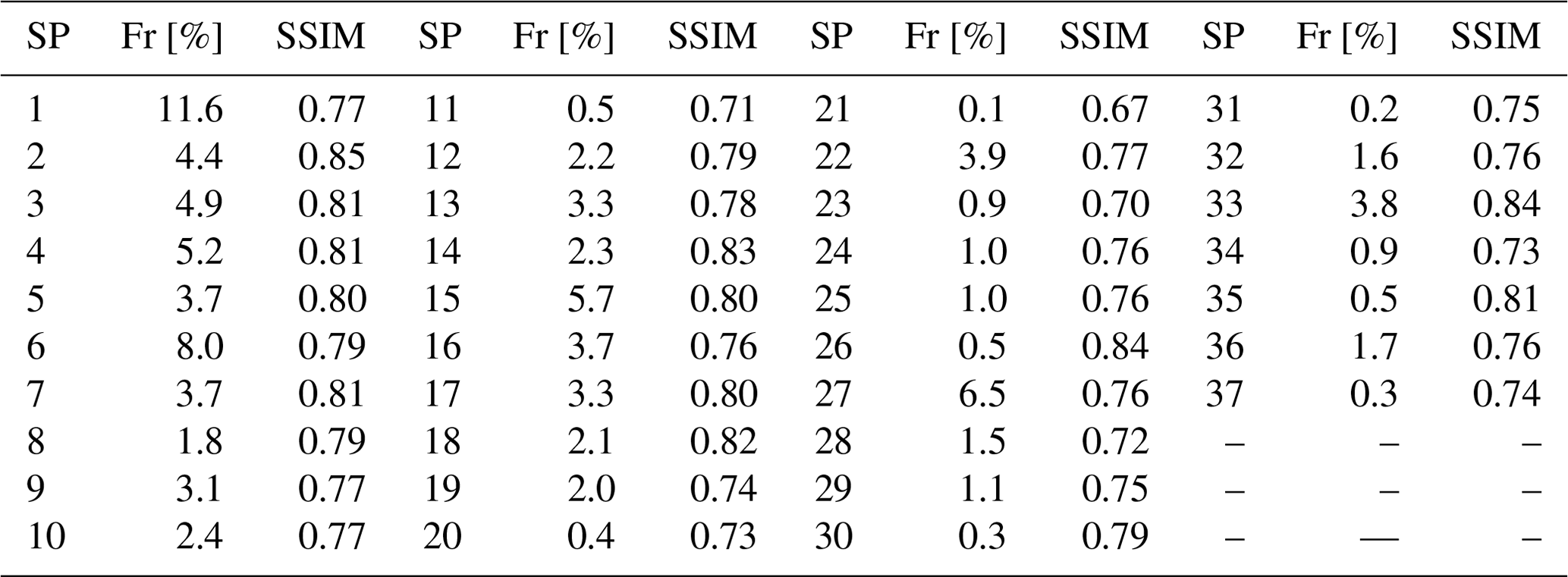
Figure 13 illustrates medoids and centroids for the five most frequent SP classes. As expected, each medoid has a higher amplitude of anomalies and the corresponding centroid shows essentially the same pattern but with weaker anomalies. The mean absolute difference (the sum of absolute differences between each element in the class and its medoid) between the two shows the highest values at the locations of strong amplitudes in the medoid fields and lower values at locations on “edges” of synoptic patterns. This is expected because the covariance term of SSIM (Eq. 3) penalizes a displacement of anomalies stronger than a mismatch of anomalies' amplitudes, i.e. steers the clustering method to prefer correctly placed anomalies over their correctly estimated amplitudes (by a false placement). Figure 13 shows the high similarity between the class medoids and their centroids and indicates that these classes are not snowballs: although the classes may have many members, they show pronounced and similar (within the class) structural patterns. This illustrates that the clustering method sensitively groups SP patterns with similar composition of the anomalies into classes using the SSIM as a similarity measure for pairs of geopotential fields.
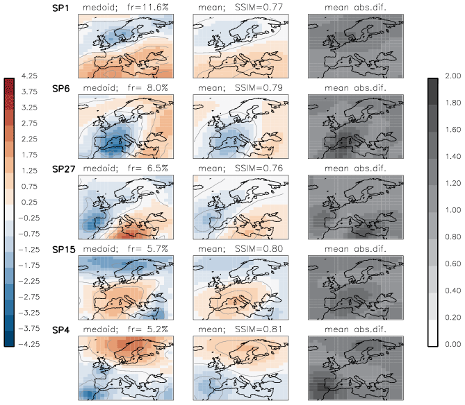
Figure 13Medoids (left column), means or centroids (centre column), and their mean absolute difference (right column) for the five most frequent SP classes. The frequency of each SP class is shown on top of each medoid plot, and the SSIM between the medoid and centroid is shown on the top of each plot of the mean.
We compute maps of exceedance probabilities for two variables – daily near-surface air temperature (tas) and daily total precipitation (pr) – for each synoptic class using maps of exceedance of the 90th percentile for days in corresponding clusters. The map of exceedance probability computed for each class is limited to the area of Germany only as we were able to validate these data using national observations as data sources. Figure 14 shows the maps of exceedance probabilities of the 90th percentile for temperature and precipitation affiliated with four exemplary synoptic classes. The class SP5, not a very rare one with occurrence of 3.7 % in the data, has no indication of exceptionally warm or wet weather as both maps of exceedance probability remain “empty” (no exceedance). For the class SP2 the map of exceedance probability for precipitation shows a frequent exceedance of the 90th percentile everywhere in Germany, with a higher probability in the southern region. The class SP35, one of the rare classes with only 0.5 % of data, appears to be frequently “hot”. The class SP29, also a rare one, frequently exhibits warm and wet weather conditions.
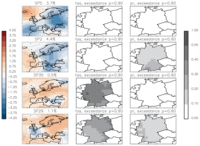
Figure 14Examples of synoptic classes and corresponding maps of exceedance probability for temperature (tas) and precipitation (pr).
Maps of exceedance probabilities for all classes are shown in the Supplement (Figs. S3–S7). Some clusters show no exceedances of the 90th percentile for either variable (SP3, 5, 9, 14, 17, 37), but some others do. Apart from the types of extreme events, which materialize through persistence of possibly not very rare circulation types (SP 1, 2, 6, 7, 15), there are others that are related to rare circulation patterns. Rare classes (with occurrence of less than 2 % in total data) SP 25, 28, 29, 30, 34, and 35 are often very warm. Rare classes SP 19, 20, 21, 23, 24, 29, 30, 31, 32, and 36 show high probabilities of intense precipitation. Precipitation is an especially “difficult” variable to evaluate in models. Dry–wet biases in models may result from bad physical parameterizations and/or from model inability to reproduce the correct synoptic pattern. Therefore, knowing that a particular synoptic pattern often goes along with strong precipitation, we can check if a model is able to reproduce this pattern or not. This knowledge would help to attribute precipitation errors to errors in models physics or dynamics.
In Fig. 15 we show examples of the three statistics: histogram of class frequencies HIST, class-to-class transition matrix TRANSIT, and matrix of persistence PERSIST of each class for 1–8 d. We chose to present these statistics for only three datasets – the reference and two models – for demonstration purposes. Figure 15a shows the large spread of frequencies of SP classes that conditions high spread in frequencies of transition matrices (Fig. 15b) and persistence matrices (Fig. 15c).
As we suggest using the statistics HIST, TRANSIT, and PERSIST for evaluation of climate models, a question on the robustness of these statistics may arise. We take 40 subsamples (30 years each) of the original ERA-Interim full dataset of 1979–2018 and assign these data to the final 37 synoptic classes. For each statistic we compute the mean and the standard deviation (SD) of these 40 resamples. As a very rough, zeroth-order check of robustness we compare the estimated values in the frequency histograms and the TRANSIT/PERSIST matrices with 2 times their resampling standard deviation. We discuss the results of this analysis of robustness in detail in the Supplement (“Analysis of the robustness of the estimates for the statistics HIST/TRANSIT/PERSIST”).
For evaluation of CMIP6 climate historical simulations, we assign each model's output to the set of reference SP classes and compute the Jensen–Shannon distance (Eq. 16) for this model to the reference. As each class is represented by its medoid, the class separation is sharper and the assignment of data samples less ambiguous compared to the common practice of using centroids. The attribution of each data element to a class is done using SSIM with respect to the class medoids.
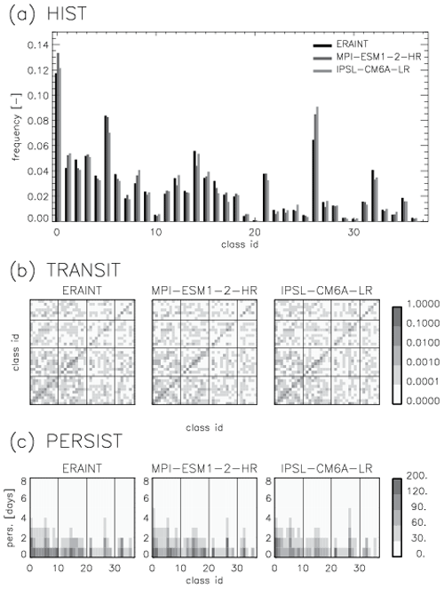
Figure 15Examples of statistics for the reference data and two CMIP6-models: (a) HIST – histogram of frequencies for each SP class; (b) TRANSIT matrices for each pair of SP classes; where diagonal elements show transition for the same class, i.e. persistence, (c) PERSISTENCE matrices that show number of events when each SP class persisted for 1, 2, 8 d (this statistic is shown in absolute values – non-normalized – for better readability).
The Jensen–Shannon distance (JS) is computed for the one-dimensional statistics (HIST, HISTDJF, HISTMAM, HISTJJA, HISTSON) as well as for the two-dimensional TRANSIT and PERSIST between the two probability distributions for each model and the reference. Resulting values of JS (Table 3) can be combined to suit objectives of the model evaluation; for example, seasonally separated JS(HISTDJF), JS(HISTMAM), and JS(HISTJJA), JS(HISTSON) can be used in evaluating seasonal frequencies of synoptic patterns and JS(PERSIST) for evaluating of the duration of synoptic patterns. In this paper, we equally weight all JSs and compute the mean Jensen–Shannon distance (Table 3). A Jensen–Shannon distance of 0.0 indicates the match between the model and the reference. The benchmark for this study: the mean Jensen–Shannon distance for the alternative reanalysis NCEP1 is 0.034 and can be viewed as the best possible JS for a model.
Table 3CMIP6 models and their Jensen–Shannon distances (JSs). The mean Jensen–Shannon distance (mean JS) is computed for each model as the mean of its individual JSs for each model statistic. The last two rows contain the mean and the standard deviation (SD) of all JSs for the same statistic across 32 CMIP6 models.
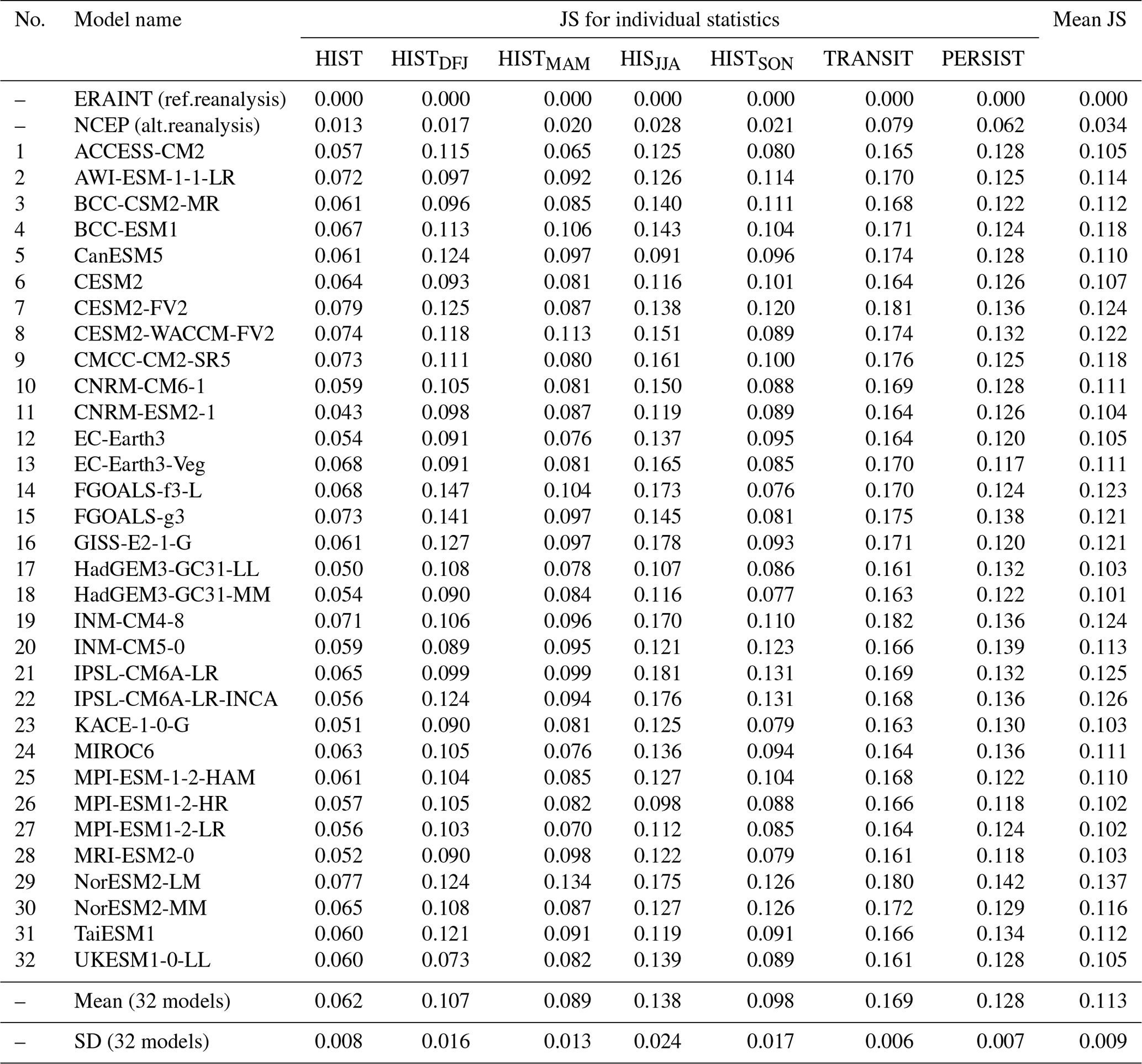
The mean Jensen–Shannon distance, meanJS, indicates how well the respective model captures the synoptic circulation in the reference data, ERA-Interim (smaller distance means a better match between the model and the reference, and vice versa). This distance metric can be easily transformed into a quality index using the formulae of Sanderson et al. (2015) and, together with quality indices for scalar variables, can be used for ranking the climate model simulations and as an evaluation measure. For example, the climate simulation NorESM2-LM seems to underperform all other models (mean JS =0.137), whereas other models show lower values (i.e. smaller distances to the reference statistics). Such a diagnostic is a useful complement for model evaluation: poor quality scores from evaluation of synoptic patterns should be seen as a warning prior to analysing scalar variables.
We presented a new two-stage classification method that uses the structural similarity index measure (SSIM) to build classifications of synoptic circulation patterns, which are described by geopotential anomaly at the level of 500 hPa. This classification method produces a set of well-separated, consistent, and representative classes. The algorithm demonstrated its robustness against temporal variability and the spatial resolution of the data. It classifies all input data fields without pre-filtering and pre-initialization of classes, and it builds structurally different classes with inter-class homogeneity. While explaining the procedure of developing the two-stage classification algorithm, we demonstrated the disadvantage of using the classical clustering algorithm k-means and the MSE as a distance measure for cluster building when classifying meteorological fields such as geopotential. We hope this demonstration helps users and developers of classification methods to be careful with interpreting their results and to be conscious that some problems (such as snowballing) may be avoided by simple modifications of the clustering algorithm as illustrated in this paper.
The important strength of the new classification method is its applicability to any region on the globe with no requirements of prior knowledge about weather types in that region. The applicability of our classification method to any region allows evaluation of models quasi-globally as is done by Cannon (2020) for evaluation of CMIP5 and CMIP6 models in six continental-scale regions (or more).
In this paper we describe the method – the recipe – to build a set of synoptic classes. We do not propose an “optimal classification” of synoptic patterns for all purposes. Depending on the purpose of classification, the presented classification method can be extended (from the single variable – geopotential anomaly at 500 hPa) to multiple variables by either targeting the optimization algorithm on a vector of similarity values or defining the SSIM for vector-valued variables.
We apply the new method to the ERA-Interim reanalysis data and build a set of synoptic classes (application of the classification method to other datasets may build other sets of synoptic classes). We demonstrate that separating rare classes may be useful for diagnostics of extreme weather events affiliated with these classes. Here we clearly make use of multiple synoptic classes as only a few of them would hamper such an attribution.
As an example, we use this set of classes to evaluate the performance of 32 global CMIP6 climate models in the CORDEX-EU domain. Model data were attributed to the reference set of classes and statistical parameters (frequency of occurrence of each pattern, frequency of transitions from one pattern to another, persistence of each pattern) were computed for these models. We compared these statistical parameters to the parameters computed from the reference data, calculating the Jensen–Shannon distance metric, and suggest using it to compute a quality index (Sanderson et al., 2015) in evaluation routines for climate models as an additional diagnostic measure. Using the distance metric proposed in this study would help to avoid misinterpretations in model evaluation such as “the right results for the wrong reasons” – when a good match of scalar variables (temperature, precipitation, etc.) between a model and the reference is achieved but the distance metric for synoptic patterns alerts us to poor model performance. We believe that the use of such a distance metric for synoptic patterns as proposed in this study would improve evaluating routines currently used for climate models and may give valuable feedback for model developers. We emphasize readers' attention here: the evaluation of model dynamics performed using synoptic classifications should not replace but complement (!) existing evaluation routines that use scalar variables and other metrics. Another application of the synoptic classes in the evaluation of climate models is the so-called “weather-pattern-based model evaluation” (Nigro et al., 2011). Surface climate model data are analysed conditionally for each class: this allows for the determination of model errors as a function of synoptic class and can highlight if certain errors occur under some synoptic situations and not others. Alternatively to evaluation, other applications of the two-stage classification are possible. A linkage of synoptic classes to extreme weather could be used to improve predictability of numerical models as was done by Nguyen-Le and Yamada (2019), who classified anomalous weather patterns associated with heavy rainfall in Thailand and implemented classification results into a global spectral model (GSM) of the Japan Meteorological Agency, improving the forecast skill with a lead time up to 3 d. However, we doubt that using synoptic classes in the form of a “precursor” for particular weather events would be the best-suited method for improving weather forecasts beyond a 3 d lead time.
The ERA-Interim reanalysis data are available at https://www.ecmwf.int/en/forecasts/dataset/ecmwf-reanalysis-interim (Dee et al., 2001). The NCEP1 reanalysis data are available at https://psl.noaa.gov/data/gridded/data.ncep.reanalysis.html (Kalnay et al., 1996).
The Global Climate Model data used in this study are part of the World Climate Research Programme's (WCRP) 6th Coupled Model Intercomparison Project (CMIP6) open-access data, accessed through the Earth System Grid Federation (https://esgf-node.llnl.gov/search/cmip6/, ESGF, 2024).
The supplement related to this article is available online at: https://doi.org/10.5194/esd-15-607-2024-supplement.
KW and CD designed the methods. CD modified the structural similarity index metric (SSIM) to be applicable to mixed-sign data as presented in this study. KW developed the code in Fortran, performed classifications, and prepared the paper with contributions from all co-authors.
The contact author has declared that none of the authors has any competing interests.
This service is based on data and products of the European Centre for Medium-Range Weather Forecasts (ECMWF).
Publisher's note: Copernicus Publications remains neutral with regard to jurisdictional claims made in the text, published maps, institutional affiliations, or any other geographical representation in this paper. While Copernicus Publications makes every effort to include appropriate place names, the final responsibility lies with the authors.
This paper was edited by Gabriele Messori and reviewed by three anonymous referees.
Adams, R. E., Lee, C. C., Smith, E. T., and Sheridan, S. C.: The relationship between atmospheric circulation patterns and extreme temperature events in North America, Int. J. Climatol., 41, 92–103, https://doi.org/10.1002/joc.6610, 2020.
Baker, A. H., Pinardy, A., and Hammerlingy, D. M.: DSSIM: a structural similarity index for floating-point data, IEEE Transactions on Visualization and Computer Graphics (Early Access), 1–13, https://doi.org/10.1109/TVCG.2023.3332843, 2022.
Baur, F.: Einführung in die Grosswetterkunde (En: Introduction into Large Scale Weather), Dieterich Verlag, Wiesbaden, Germany, https://doi.org/10.1002/qj.49707633014, 1948.
Beck, C., Jacobeit, J., and Jones, P. D.: Frequency and within-type variations of large-scale circulation types and their effects on low-frequency climate variability in central europe since 1780, Int. J. Climatol., 27, 473–491, https://doi.org/10.1002/joc.1410, 2007.
Cannon, A. J.: Semi-supervised multivariate regression trees: putting the `circulation' back into a `circulation-to-environment' synoptic classifier, Int. J. Climatol., 32, 2251–2254, https://doi.org/10.1002/joc.2417, 2012.
Cannon, A. J.: Reductions in daily continental-scale atmospheric circulation biases between generations of global climate models: CMIP5 to CMIP6, Environ. Res. Lett., 15, 064006, https://doi.org/10.1088/1748-9326/ab7e4f, 2020.
Cannon, A. J., Whitfield, P. H., and Lord, E. R.: Synoptic Map-Pattern Classification Using Recursive Partitioning and Principal Component Analysis, Mon. Weather Rev., 130, 1187–1206, 2001.
Cassano, E. N., Lynch, A. H., Cassano, J. J., and Koslow, M. R.: Classification of synoptic patterns in the western Arctic associated with extreme events at Barrow, Alaska, USA, Clim. Res., 30, 83–97, https://doi.org/10.3354/cr030083, 2006.
D'Urso, P. and Massari, R.: Fuzzy clustering of mixed data, Inform. Sciences, 505, 513–534, https://doi.org/10.1016/j.ins.2019.07.100, 2019.
Dee, D. P., Uppala, S. M., Simmons, A. J., Berrisford, P., Poli, P., Kobayashi, S., Andrae, U., Balmaseda, M. A., Balsamo, G., Bauer, P., Bechtold, P., Beljaars, A. C. M., van de Berg, L., Bidlot, J., Bormann, N., Delsol, C., Dragani, R., Fuentes, M., Geer, A. J., Haimberger, L., Healy, S. B., Hersbach, H., Hólm, E. V., Isaksen, L., Kållberg, P., Köhler, M., Matricardi, M., McNally, A. P., Monge-Sanz, B. M., Morcrette, J. J., Park, B. K., Peubey, C., de Rosnay, P., Tavolato, C., Thépaut, J. N., and Vitart, F.: The ERA-Interim reanalysis: configuration and performance of the data assimilation system, Q. J. Roy. Meteor. Soc., 137, 553–597, https://doi.org/10.1002/qj.828, 2011 (data available at: https://www.ecmwf.int/en/forecasts/dataset/ecmwf-reanalysis-interim, last access: 8 May 2024).
Díaz-Esteban, Y., Raga, G. B., and Díaz Rodríguez, O. O.: A Weather-Pattern-Based Evaluation of the Performance of CMIP5 Models over Mexico, Climate, 8, 1–18, https://doi.org/10.3390/cli8010005, 2020.
Dittmann, E., Barth, S., Lang, J., and Müller-Westermeier, G.: Objektive Wetterlagenklassifikation (En: Objective weather type classification), Deutscher Wetterdienst, Offenbach am Main, Germany, ISBN 3-88148-316-0, 1995.
Dorrington, J. and Strommen, K. J.: Jet Speed Variability Obscures Euro-Atlantic Regime Structure, Geophys. Res. Lett., 47, e2020GL087907, https://doi.org/10.1029/2020gl087907, 2020.
ESGF: CMIP6, [data set], https://aims2.llnl.gov/search/cmip6/, last access: 15 May 2024.
Eyring, V., Bony, S., Meehl, G. A., Senior, C. A., Stevens, B., Stouffer, R. J., and Taylor, K. E.: Overview of the Coupled Model Intercomparison Project Phase 6 (CMIP6) experimental design and organization, Geosci. Model Dev., 9, 1937–1958, https://doi.org/10.5194/gmd-9-1937-2016, 2016.
Fabiano, F., Christensen, H. M., Strommen, K., Athanasiadis, P., Baker, A., Schiemann, R., and Corti, S.: Euro-Atlantic weather Regimes in the PRIMAVERA coupled climate simulations: impact of resolution and mean state biases on model performance, Clim. Dynam., 54, 5031–5048, https://doi.org/10.1007/s00382-020-05271-w, 2020.
Falkena, S. K. J., Wiljes, J., Weisheimer, A., and Shepherd, T. G.: Detection of interannual ensemble forecast signals over the North Atlantic and Europe using atmospheric circulation regimes, Q. J. Roy. Meteor. Soc., 148, 434–453, https://doi.org/10.1002/qj.4213, 2021.
Fettweis, X., Mabille, G., Erpicum, M., Nicolay, S., and den Broeke, M. V.: The 1958–2009 Greenland ice sheet surface melt and the mid-tropospheric atmospheric circulation, Clim. Dynam., 36, 139–159, https://doi.org/10.1007/s00382-010-0772-8, 2010.
Fulton, D. J. and Hegerl, G. C.: Testing Methods of Pattern Extraction for Climate Data Using Synthetic Modes, J. Climate, 34, 7645–7660, https://doi.org/10.1175/jcli-d-20-0871.1, 2021.
Gerstengarbe, F.-W. and Werner, P. C.: Katalog der Großwetterlagen Europas nach Paul Hess und Helmut Brezowski 1881–1992, Deutscher Wetterdienst, Offenbach am Main, Germany, 113, 1–249, ISSN 2194-5969, 1993.
Gervais, M., Atallah, E., Gyakum, J. R., and Tremblay, L. B.: Arctic Air Masses in a Warming World, J. Climate, 29, 2359–2373, https://doi.org/10.1175/jcli-d-15-0499.1, 2016.
Gleckler, P. J., Taylor, K. E., and Doutriaux, C.: Performance metrics for climate models, J. Geophys. Res., 113, D06104, https://doi.org/10.1029/2007jd008972, 2008.
Grams, C. M., Beerli, R., Pfenninger, S., Staffell, I., and Wernli, H.: Balancing Europe's wind power output through spatial deployment informed by weather regimes, Nat. Clim. Change, 7, 557–562, https://doi.org/10.1038/nclimate3338, 2017.
Hannachi, A., Straus, D. M., Franzke, C. L. E., Corti, S., and Woollings, T.: Low-frequency nonlinearity and regime behavior in the Northern Hemisphere extratropical atmosphere, Rev. Geophys., 55, 199–234, https://doi.org/10.1002/2015rg000509, 2017.
Herrera-Lormendez, P., Mastrantonas, N., Douville, H., Hoy, A., and Matschullat, J.: Synoptic circulation changes over Central Europe from 1900 to 2100: Reanalyses and Coupled Model Intercomparison Project phase 6, Int. J. Climatol., 42, 4062–4077, https://doi.org/10.1002/joc.7481, 2021.
Hess, P. and Brezowsky, H.: Katalog der Großwetterlagen Europas, Deutscher Wetterdienst Zentralamt Bad Kissingen, 1952.
Hewitson, B. C. and Crane, R. G.: Self-organizing maps: applications to synoptic climatology, Clim. Res., 22, 13–26, https://doi.org/10.3354/cr022013, 2002.
Hochman, A., Messori, G., Quinting, J. F., Pinto, J. G., and Grams, C. M.: Do Atlantic-European Weather Regimes Physically Exist?, Geophys. Res. Lett., 48, e2021GL095574, https://doi.org/10.1029/2021gl095574, 2021.
Huth, R.: An Intercomparison of Computer-assisted Circulation Classification Methods. International Journal of Climatology, Int. J. Climatol., 16, 893–922, 1996.
Huth, R.: A circulation classi®cation scheme applicable in GCM studies, Theor. Appl. Climatol., 67, 1–18, https://doi.org/10.1007/s007040070012, 2000.
Huth, R. and Beranová, R.: How to Recognize a True Mode of Atmospheric Circulation Variability, Earth Space Sci., 8, e2020EA001275, https://doi.org/10.1029/2020ea001275, 2021.
Huth, R., Beck, C., Philipp, A., Demuzere, M., Zbigniew, U., Cahynová, M., Kyselý, J., and Tveito, O. E.: Classifications of Atmospheric Circulation Patterns, Recent Advances and Applications, Trends and Directions in Climate Research, Ann. NY Acad. Sci., 1146, 105–152, 2008.
James, P. M.: An objective classification method for Hess and Brezowsky Grosswetterlagen over Europe, Theor. Appl. Climatol., 88, 17–42, https://doi.org/10.1007/s00704-006-0239-3, 2006.
James, P. and Ostermöller, J.: GWL-REA: An improved method for classifying Hess-Brezowksy Grosswetterlagen based on pattern correlations in combination with Lamb Weather Type statistics, EMS Annual Meeting 2022, Bonn, Germany, 5–9 Sep 2022, EMS2022-415, https://doi.org/10.5194/ems2022-415, 2022.
Jiang, N., Cheung, K., Luo, K., Beggs, P. J., and Zhou, W.: On two different objective procedures for classifying synoptic weather types over east Australia, Int. J. Climatol., 32, 1475–1494, https://doi.org/10.1002/joc.2373, 2011.
Kalnay, E., Kanamitsu, M., Kistler, R., Collins, W., Deaven, D., Gandin, L., Iredell, M., Saha, S., White, G., Woollen, J., Zhu, Y., Chelliah, M., Ebisuzaki, W., Higgins, W., Janowiak, J., Mo, K. C., Ropelewski, C., Wang, J., Leetmaa, A., Reynolds, R., Jenne, R., and Joseph, D.: The NCEP/NCAR 40-Year Reanalysis Project, B. Am. Meteor. Soc., 77, 437–471, https://doi.org/10.1175/1520-0477(1996)077<0437:TNYRP>2.0.CO;2, 1996 (data available at: https://psl.noaa.gov/data/gridded/data.ncep.reanalysis.html, last access: 8 May 2024).
Kaufman, L. and Rousseeuw, P. J.: Partitioning Around Medoids (Program PAM), in: Finding Groups in Data: An Introduction to Cluster Analysis, Wiley Series in Probability and Statistics, John Wiley & Sons, Inc., 68–125, https://doi.org/10.1002/9780470316801.ch2, 1990.
Kohonen, T.: Self-Organizing Maps Springer Series in Information Sciences (SSINF), 30, Springer Berlin, Heidelberg, https://doi.org/10.1007/978-3-642-56927-2, 2001.
Lamb, H. H.: British Isles weather types and a register of the daily sequence of circulation patterns 1861–1971, Geophysical memoirs, London, H.M. Stationery Office 1972, Vol. 16, 85 pp., 1972.
Lauscher, F.: Klimatologische Synoptik Österreichs mittels der ostalpinen Wetterlagenklassifikation (En: (Synoptic Climatology of Austria based on the Eastern-Alpine Weather Type Classification), Zentralanstalt für Meteorologie und Geodynamik (ZAMG), Wienna, Austria, 64, 302, 1985.
Lee, C. C. and Sheridan, S. C.: A six-step approach to developing future synoptic classifications based on GCM output, Int. J. Climatol., 32, 1792–1802, https://doi.org/10.1002/joc.2394, 2012.
Meehl, G. A., Boer, G. J., Covey, C., Latif, M., and Stouffer, R. J.: Intercomparison Makes for a Better Climate Model, Eos Science News by AGU, 78, 445–446, https://doi.org/10.1029/97EO00276 1997.
Meehl, G. A., Boer, G. J., Covey, C., Latif, M., and Stouffer, R. J.: The Coupled Model Intercomparison Project (CMIP), B. Am. Meteor. Soc., 81, 313–318, 2000.
Meehl, G. A., Covey, C., Delworth, T., Latif, M., McAvaney, B., Mitchell, J. F. B., Stouffer, R. J., and Taylor, K. E.: THE WCRP CMIP3 Multimodel Dataset: A New Era in Climate Change Research, B. Am. Meteor. Soc., 88, 1383–1394, https://doi.org/10.1175/bams-88-9-1383, 2007.
Milligan, G. W.: An algorithm for generating artificial test clusters, Psychometrika, 50, 123–127, 1985.
Mo, R., Ye, C., and Whitfield, P. H.: Application Potential of Four Nontraditional Similarity Metrics in Hydrometeorology, J. Hydrometeorol., 15, 1862–1880, https://doi.org/10.1175/jhm-d-13-0140.1, 2014.
Muñoz, Á. G., Yang, X., Vecchi, G. A., Robertson, A. W., and Cooke, W. F.: A Weather-Type-Based Cross-Time-Scale Diagnostic Framework for Coupled Circulation Models, J. Climate, 30, 8951–8972, https://doi.org/10.1175/jcli-d-17-0115.1, 2017.
Nguyen-Le, D. and Yamada, T. J.: Using Weather Pattern Recognition to Classify and Predict Summertime Heavy Rainfall Occurrence over the Upper Nan River Basin, Northwestern Thailand, Weather Forecast., 34, 345–360, https://doi.org/10.1175/waf-d-18-0122.1, 2019.
Nigro, M. A., Cassano, J. J., and Seefeldt, M. W.: A Weather-Pattern-Based Approach to Evaluate the Antarctic Mesoscale Prediction System (AMPS) Forecasts: Comparison to Automatic Weather Station Observations, Weather Forecast., 26, 184–198, https://doi.org/10.1175/2010waf2222444.1, 2011.
Perez, J., Menendez, M., Mendez, F. J., and Losada, I. J.: Evaluating the performance of CMIP3 and CMIP5 global climate models over the north-east Atlantic region, Clim. Dynam., 43, 2663–2680, https://doi.org/10.1007/s00382-014-2078-8, 2014.
Philipp, A., Bartholy, J., Beck, C., Erpicum, M., Esteban, P., Fettweis, X., Huth, R., James, P., Jourdain, S., Kreienkamp, F., Krennert, T., Lykoudis, S., Michalides, S. C., Pianko-Kluczynska, K., Post, P., Álvarez, D. R., Schiemann, R., Spekat, A., and Tymvios, F. S.: Cost733cat – A database of weather and circulation type classifications, Phys. Chem. Earth, 35, 360–373, https://doi.org/10.1016/j.pce.2009.12.010, 2010.
Radiæ, V. and Clarke, G. K. C.: Evaluation of IPCC Models' Performance in Simulating Late-Twentieth-Century Climatologies and Weather Patterns over North America, J. Climate, 24, 5257–5274, https://doi.org/10.1175/jcli-d-11-00011.1, 2011.
Riediger, U. and Gratzki, A.: Future weather types and their influence on mean and extreme climate indices for precipitation and temperature in Central Europe, Meteorol. Z., 23, 231–252, https://doi.org/10.1127/0941-2948/2014/0519, 2014.
Sanderson, B. M., Knutti, R., and Caldwell, P.: A Representative Democracy to Reduce Interdependency in a Multimodel Ensemble, J. Climate, 28, 5171–5194, https://doi.org/10.1175/jcli-d-14-00362.1, 2015.
Schubert, E. and Rousseeuw, P. J.: Fast and eager k-medoids clustering: O(k) runtime improvement of the PAM, CLARA, and CLARANS algorithms, Inform. Systems, 101, 101804, https://doi.org/10.1016/j.is.2021.101804, 2021.
Taylor, K. E., Stouffer, R. J., and Meehl, G. A.: An Overview of CMIP5 and the Experiment Design, B. Am. Meteor. Soc., 93, 485–498, https://doi.org/10.1175/bams-d-11-00094.1, 2012.
Tveito, O. E., Huth, R., Philipp, A., Post, P., Pasqui, M., Esteban, P., Beck, C., Demuzere, M., and Prudhomme, C.: COST Action 733 Harmonization and Application of Weather Type Classifications for European Regions, https://www.researchgate.net/publication/303863197_COST_Action_733_Harmonization_and_Application_of_Weather_Type_Classifications_for_European_Regions (last access: 13 May 2024), 2016.
Wang, Z. and Bovik, A. C.: Mean squared error: Love it or leave it? A new look at Signal Fidelity Measures, IEEE Signal Proc. Mag., 26, 98–117, https://doi.org/10.1109/msp.2008.930649, 2009.
Wang, Z., Bovik, A. C., Sheikh, H. R., and Simoncelli, E. P.: Image quality assessment: from error visibility to structural similarity, IEEE T. Image Process., 13, 600–612, https://doi.org/10.1109/tip.2003.819861, 2004.
Yarnal, B., Comrie, A. C., Frakes, B., and Brown, D. P.: Developments and prospects in synoptic climatology, Int. J. Climatol., 21, 1923–1950, https://doi.org/10.1002/joc.675, 2001.
- Abstract
- Introduction
- Data
- Method
- Results
- Weather extremes affiliated with the synoptic classes
- Statistics and the Jensen–Shannon distance metric for evaluation of CMIP6 historical climate simulations
- Conclusions
- Code and data availability
- Author contributions
- Competing interests
- Disclaimer
- Review statement
- References
- Supplement
The requested paper has a corresponding corrigendum published. Please read the corrigendum first before downloading the article.
- Article
(1919 KB) - Full-text XML
- Corrigendum
-
Supplement
(3192 KB) - BibTeX
- EndNote
- Abstract
- Introduction
- Data
- Method
- Results
- Weather extremes affiliated with the synoptic classes
- Statistics and the Jensen–Shannon distance metric for evaluation of CMIP6 historical climate simulations
- Conclusions
- Code and data availability
- Author contributions
- Competing interests
- Disclaimer
- Review statement
- References
- Supplement