the Creative Commons Attribution 4.0 License.
the Creative Commons Attribution 4.0 License.
 | 24 Apr 2024
Dependency of the impacts of geoengineering on the stratospheric sulfur injection strategy – Part 2: How changes in the hydrological cycle depend on the injection rate and model used
Daniele Visioni
Ulrike Niemeier
Simone Tilmes
Harri Kokkola
This is the second of two papers in which we study the dependency of the impacts of stratospheric sulfur injections on the model and injection strategy used. Here, aerosol optical properties from simulated stratospheric aerosol injections using two aerosol models (modal scheme M7 and sectional scheme SALSA), as described in Part 1 (Laakso et al., 2022), are implemented consistently into the EC-Earth, MPI-ESM and CESM Earth system models (ESMs) to simulate the climate impacts of different injection rates ranging from 2 to 100 Tg(S) yr−1. Two sets of simulations were run with the three ESMs: (1) regression simulations, in which an abrupt change in CO2 concentration or stratospheric aerosols over pre-industrial conditions was applied to quantify global mean fast temperature-independent climate responses and quasi-linear dependence on temperature, and (2) equilibrium simulations, in which radiative forcing of aerosol injections with various magnitudes compensated for the corresponding radiative forcing of CO2 enhancement to study the dependence of precipitation on the injection magnitude. The latter also allow one to explore the regional climatic responses. Large differences in SALSA- and M7-simulated radiative forcing in Part 1 translated into large differences in the estimated surface temperature and precipitation changes in ESM simulations; for example, an injection rate of 20 Tg(S) yr−1 in CESM using M7-simulated aerosols led to only 2.2 K global mean cooling, while EC-Earth–SALSA combination produced a 5.2 K change. In equilibrium simulations, where aerosol injections were utilized to offset the radiative forcing caused by an atmospheric CO2 concentration of 500 ppm, the decrease in global mean precipitation varied among models, ranging from −0.7 % to −2.4 % compared with the pre-industrial climate. These precipitation changes can be explained by the fast precipitation response due to radiation changes caused by the stratospheric aerosols and CO2, as the global mean fast precipitation response is shown to be negatively correlated with global mean atmospheric absorption. Our study shows that estimating the impact of stratospheric aerosol injection on climate is not straightforward. This is because the simulated capability of the sulfate layer to reflect solar radiation and absorb long-wave radiation is sensitive to the injection rate as well as the aerosol model used to simulate the aerosol field. These findings emphasize the necessity for precise simulation of aerosol microphysics to accurately estimate the climate impacts of stratospheric sulfur intervention. This study also reveals gaps in our understanding and uncertainties that still exist related to these controversial techniques.
- Article
(8551 KB) - Full-text XML
- Companion paper
-
Supplement
(12558 KB) - BibTeX
- EndNote


One of the most studied solar radiation modification (SRM) techniques is stratospheric aerosol intervention (SAI), which has the intent of producing a layer of aerosols that reflects solar radiation back to space. Such techniques could artificially decrease the radiative imbalance caused by increased greenhouse gas (GHG) emissions and, in theory, maintain radiative balance. However, in this theoretical case, all impacts would not be compensated for. As GHGs suppress the outgoing long-wave (LW) radiation, SAI compensates for GHG-induced radiative imbalance by altering mostly solar short-wave (SW) radiation. The magnitude of SRM could be adjusted to compensate for GHG-induced radiative flux change at the top of the atmosphere (TOA), although not without changes in the atmospheric energy budget, as the spatiotemporal structure of SW radiative fluxes differs from LW fluxes in the atmosphere. Thus, this would lead to several consequences, such as a decrease in global mean precipitation and unevenly distributed temperature change compared with a climate without an increase in CO2 and SAI (e.g. Visioni et al., 2021; Laakso et al., 2020; Tilmes et al., 2013). The extent of these impacts is influenced not only by the level of GHG increase in the atmosphere but also by the interaction of aerosol fields with SW and LW radiation. This interaction is further dependent on the aerosols' optical properties, which, as demonstrated in Laakso et al. (2022), are closely associated with the modelling of aerosol microphysics in climate models.
Most studies simulate injections of SO2 for SAI. In this imitation of large volcanic eruptions, injected SO2 oxidizes to sulfuric acid and then either forms new particles or condenses on existing ones. Radiative properties of sulfate aerosols depend strongly on the size of these aerosols and, thus, are sensitive to ambient conditions during injections (background conditions and injection strategy). The sensitivity to microphysical processes (nucleation, coagulation, and condensation) in climate models depends very much on how such processes are modelled. Several studies on SAI using SO2 injections show that, for a fixed injection area, radiative forcing efficiency (i.e. radiative forcing or injection rate) decreases with a larger magnitude of injections (Heckendorn et al., 2009; Pierce et al., 2010; Niemeier et al., 2011). However, the magnitude of this reduction in the forcing efficiency and the predicted radiative forcing are considerably different between studies and models. In Laakso et al. (2022), hereafter referred as Part 1, we simulated different injection rates using both a sectional aerosol model (SALSA) and a modal model (M7) within the same climate model, showing that there are indeed significant differences in the radiative forcing of SAI depending on how aerosol microphysics are simulated. In the case of continuous SO2 injections to the Equator with injection rates of 1–100 Tg(S) yr−1, an 88 %–154 % higher global mean all-sky net radiative forcing is produced when simulated with SALSA compared with M7.
In the case of SAI with sulfate, injected aerosols would not only scatter solar radiation but also absorb SW and LW radiation. In Part 1, we showed that, while SW radiative forcing (negative, i.e cooling impact) saturates considerably with the injection rate, the relation of LW radiative forcing (positive, i.e warming impact) and injection rate is more linear (Niemeier and Timmreck, 2015). This means that the contribution of LW radiation to the total radiative forcing becomes larger for larger injection rates: in SALSA simulations, LW radiation forcing compensated for between 10 % and 28 % of the SW radiative forcing with an injection rate of 1–100 Tg(S) yr−1, whereas this range was 24 %–57 % for the M7 simulation. This also has implications for how these radiative forcing values translate to climate impacts because, as a side-effect, aerosols are absorbing radiation and are warming the atmosphere. The impact of LW absorption becomes stronger if larger injection rates are applied. This is also linked to how aerosols are modelled: in Part 1, SW radiative forcing was 45 %–85 % higher and LW radiative forcing was 24 %–40 % lower in simulations with SALSA compared with M7. This indicates that there would be significant differences in the simulated climate responses depending on how the aerosols are simulated. The situation is further complicated by the lack of clear criteria for selecting the appropriate aerosol model. Observations following the 1991 Pinatubo eruption have frequently been utilized as a benchmark for evaluating models' ability to simulate stratospheric aerosols. However, a single sulfur injection, as in the case of Pinatubo, differs significantly from continuous injections, as in the case of SAI. Notably, there is a minimal difference between the M7 and SALSA model results in the simulations of the Pinatubo eruption, as detailed in Kokkola et al. (2018). Simulations using the M7 model were 60 % faster than those with SALSA, but there were some numerical limitations associated with the modes in M7 that restricted the aerosols from achieving an optimal size range for effectively scattering radiation, as noted in Laakso et al. (2022). However, the performance of the M7 results is also sensitive to the configuration of the modes, making it difficult to predict which set-up will perform well, as the performance depends on the simulated case (i.e volcanic eruption vs. SAI and different injection strategies for SAI).
Changes in atmospheric radiation also have a direct impact on precipitation. Precipitation changes can be explained by the changes in the total column atmospheric energy budget (O'Gorman et al., 2012). The atmosphere possesses a relatively low heat capacity; thus, following a perturbation, it rapidly reaches a state in which the incoming and outgoing energy fluxes to and from the atmosphere balance each other. In other words, the budget of perturbations between two atmospheric states can be expressed as follows:
where L is the latent heat of condensation, P is precipitation, RTOA and RSurf are the respective changes in the radiative fluxes at the top of the atmosphere and surface, SH is the sensible heat flux change, and δRabs is the change in absorbed radiation. Niemeier et al. (2013) showed that changes in global latent heat flux dominate changes in sensible heat flux, establishing a roughly linear relationship between precipitation and the discrepancy between the radiative imbalance at the surface and at the top of the atmosphere. Other studies have also shown that changes in precipitation are proportional to the difference between changes in radiation at the surface and in the atmosphere, i.e absorbed radiation (O'Gorman et al., 2012; Kravitz et al., 2013b; Liepert and Previdi, 2009). The atmospheric energy budget can also be utilized to represent precipitation in a transient climate. Given that radiation (and changes in atmospheric absorption) are known to be relatively linearly correlated with global mean precipitation, as evidenced by climate models (e.g Zelinka et al., 2020) and observations (Koll and Cronin, 2018), precipitation change can be approximated by a simple equation comprising temperature-dependent and temperature-independent components:
where δT is global mean temperature change, a is a constant and F represents the temperature-independent components. Within this equation, aδT accounts for all feedbacks attributable to temperature change, including the variation in surface sensible heat flux. This is often referred to as the slow precipitation response or component, which changes over a multi-year timescale alongside alterations in sea surface temperature. F is referred to as the fast precipitation response (or component) or rapid adjustment. It can be considered to include the direct radiative forcing, or precisely direct change in absorbed radiation. Thus, at the global scale, a change in global mean precipitation has been shown to be linearly dependent on the absorption part of the induced radiative forcing (Laakso et al., 2020; Myhre et al., 2017; Samset et al., 2016); therefore, a stronger atmospheric absorption of radiation is linked to a decrease in global mean precipitation. Niemeier et al. (2013) investigated the impact of different SRM techniques applied at different altitudes. Their findings show that the precipitation changes predicted by Eq. (1) align closely with the precipitation changes observed in simulations. Changes in sensible heat flux within their simulations were minimal, suggesting that the calculation of precipitation based on atmospheric absorption is not influenced by the altitude at which the absorption change occurs.
In the case of solar radiation modification generally, the unambiguous impact of this is seen in model simulations in which the GHG-induced radiative imbalance is fully compensated for by SRM. Without SRM, there would be an increase in global mean precipitation, driven by a rise in temperature. However, if the temperature increase is offset by SRM, it results in an overcompensation and a decrease in global mean precipitation (e.g. Kravitz et al., 2013b). In this case, even though the GHG-induced radiative imbalance is compensated for with SAI, the radiative impact of GHG remains in the atmosphere and still absorbs LW radiation. This causes a decrease in global mean precipitation, even though there is less SW radiation for the background atmosphere to absorb due to SRM (Laakso et al., 2020). Seeley et al. (2021) studied the idea of concentrating solar dimming at the wavelengths in which water vapour has strong absorption bands. This minimized the reduction in the hydrological cycle, and simulations showed that it was able to restore mean temperature and precipitation simultaneously. However, their study was solely theoretical. The situation is more complicated when aerosols are taken into account. Presumably, there is less SW radiation to be absorbed by background atmosphere under the aerosol layer; however, as aerosols are also absorbing LW radiation, they will also slow down the hydrological cycle. Thus, several studies have shown lower global mean precipitation in simulations with SAI compared with an ideal reduction in solar radiation only with similar impacts in global mean temperature (Niemeier et al., 2013; Ferraro et al., 2014). Estimating the total impact of stratospheric aerosols on precipitation is not straightforward, as the optical properties of aerosols and their impact on SW and LW radiation depend on the size of the aerosols and the injection rate, as described above. In addition, differences in the results between the aerosol modules used is expected to translate into large differences in the consequent precipitation responses.
Here, we study how the radiative forcing simulated in Part 1 translates to changes in precipitation and temperature. We investigate how the aerosol impact on SW and LW radiation changes the atmospheric absorption and, further, the atmospheric energy budget and hydrological cycle. We also study how precipitation changes under different SAI intensities. Furthermore, we examine how these outcomes vary based on the aerosol microphysics model employed to simulate the aerosol fields as well as the Earth system model (ESM) used to simulate climate responses. Simulations are done with three different ESMs: EC-Earth, the Community Earth System Model (CESM) and the Max Planck Institute Earth System Model (MPI-ESM). We implement aerosol optical properties simulated in Part 1 into all three ESMs; thus, stratospheric aerosol optical properties are the same in all three ESMs. In this study, we only consider variations in the strategy in terms of the injection rate magnitude, although always with the same injection profile by making injections continuously to the Equator only, and ignore changes in strategy using spatial and temporal variation, as done in Part 1.
2.1 Models
2.1.1 Earth system models: EC-Earth, MPI-ESM and CESM
We used three state-of-the-art ESMs, which all include modules for the atmosphere, land and ocean. These models are the Max Planck Institute Earth System Model (MPI-ESM1.2; Mauritsen et al., 2019), the Community Earth System Model (CESM2.1.2; Danabasoglu et al., 2020) and EC-Earth (version 3.3.1; Döscher et al., 2022). These models represent a wide range of climate sensitivities (effective climate sensitivity in CO2 quadrupling experiment: MPI-ESM, 3.13 K; EC-Earth, 4.1 K; CESM, 5.15 K) present in Coupled Model Intercomparison Project Phase 6 (CMIP6) models (Zelinka et al., 2020). MPI-ESM consists of the following atmospheric models: ECHAM6.3, the Max Planck Institute Ocean Model (MPIOM, which includes the HAMOCC ocean biogeochemistry model) and the JSBACH land model. CESM 2.0 consists of the Community Atmospheric Model (CAM6), the Parallel Ocean Program (POP2) ocean model, the Community Land Model (CLM4) and the Community Ice CodE (CICE4) sea ice model. For EC-Earth, the respective atmospheric, ocean, land and ocean biochemistry models are as follows: IFS, NEMO, LPJ-GUESS and PISCES. Thus, these three ESMs do not share the same model components, and the results can be considered relatively independent of each other. However, the radiative transfer module in all three ESMs (and in the aerosol–climate model used to simulate aerosol optical properties of aerosols fields in Part 1) is based on the Rapid Radiative Transfer Model, which uses the 14 SW and 16 LW radiation bands (Döscher et al., 2022; Danabasoglu et al., 2020; Mauritsen et al., 2019). This makes implementation of optical properties of stratospheric aerosols rather straightforward. The resolution of atmosphere used in MPI-ESM, CESM and EC-Earth simulations is T63L47 (1.9°×1.9°), finite-volume 0.9°×1.25° and 32 vertical levels, and T255L91 (0.70°×0.70°), respectively.
2.1.2 ECHAM-HAMMOZ aerosol–climate model used in Part 1
Simulations in Part 1 were done with the ECHAM-HAMMOZ (ECHAM6.3-HAM2.3-MOZ1.0) aerosol–climate model (Zhang et al., 2012; Kokkola et al., 2018; Schultz et al., 2018; Tegen et al., 2019). The atmospheric model is the same as in the MPI-ESM version used in this study (Stevens et al., 2013). Simulations were performed with a T63L95 (i.e. 1.9°×1.9°) resolution, which enables one to resolve the quasi-biennial oscillation (QBO). Aerosols were simulated by two different aerosol modules: the sectional module SALSA, where aerosols are represented by 10 size bins in size space, and the modal module M7, which has 4 modes in size space. Seven-year (roughly three whole QBO cycles) simulations were done for each scenario. A more detailed description of the model is found in Laakso et al. (2022).
2.2 Implementation of stratospheric aerosol optical properties
Radiation modules in ESMs calculate the impact of aerosols on radiation via three different aerosol radiation properties: (i) aerosol optical depth (AOD) or extinction, which is a quantity that describes how aerosol interacts with the radiation; (ii) single-scattering albedo (SSA), which is the ratio of scattering efficiency to total extinction efficiency; and (iii) the asymmetry factor (ASYM). The aerosol module calculates these quantities at each grid point and radiation wavelength band based on the aerosol size and refractive indices. During the simulations with ECHAM-HAMMOZ in Part 1, AOD, SSA and ASYM were archived as monthly and zonal mean output for 14 SW bands and absorption, and AOD (absorption only) was also archived for 16 LW bands used in the radiation model. In this study, aerosol properties do not vary between years and a 7-year average of radiative properties was taken each month. These aerosol fields were implemented in MPI-ESM, CESM and EC-Earth by using them as input fields. As mentioned earlier, wavelength bands are the same in all of these models; thus, no interpolation to other wavelengths was needed. However, different resolutions were used between models; therefore, aerosols had to be interpolated to corresponding resolutions. Prescribed aerosol properties have two advantages compared with simulating prognostic aerosols in each ESM: (i) ESM simulations without a complex interactive aerosol module are computationally significantly lighter, but, this way, the impact of aerosol microphysics is nonetheless considered, and (ii) stratospheric aerosol properties are consistently implemented to all three ESMs.
2.3 Quantifying fast and slow responses
The fast temperature-independent response and the slow temperature-dependent feedback response of precipitation and radiation can be quantified using the so-called regression method (Richardson et al., 2016). The method can be used for simulations with an abrupt or step change in the climate conditions, for example, an abrupt change in the atmospheric CO2 concentration. By regressing the yearly mean variable of interest (e.g. precipitation) change against the temperature change due to the instantaneous forcing, the fast response is given as the intercept of the regression line and y axes (dT=0), whereas the temperature-dependent feedback response is the slope of the regression line (see Fig. 1). This method is built on the assumption that the variables under analysis are linearly dependent on each other. This is more or less the case, for example, for global mean radiative fluxes and precipitation (Laakso et al., 2022). Thus, this technique is a useful tool to separate the temperature-independent quantities as radiative forcing or fast precipitation response as well as effective climate sensitivity and hydrological sensitivity. As shown by Laakso et al. (2020), these quantities can be used to estimate the total global precipitation change in scenarios were SAI is used to mitigate climate change.
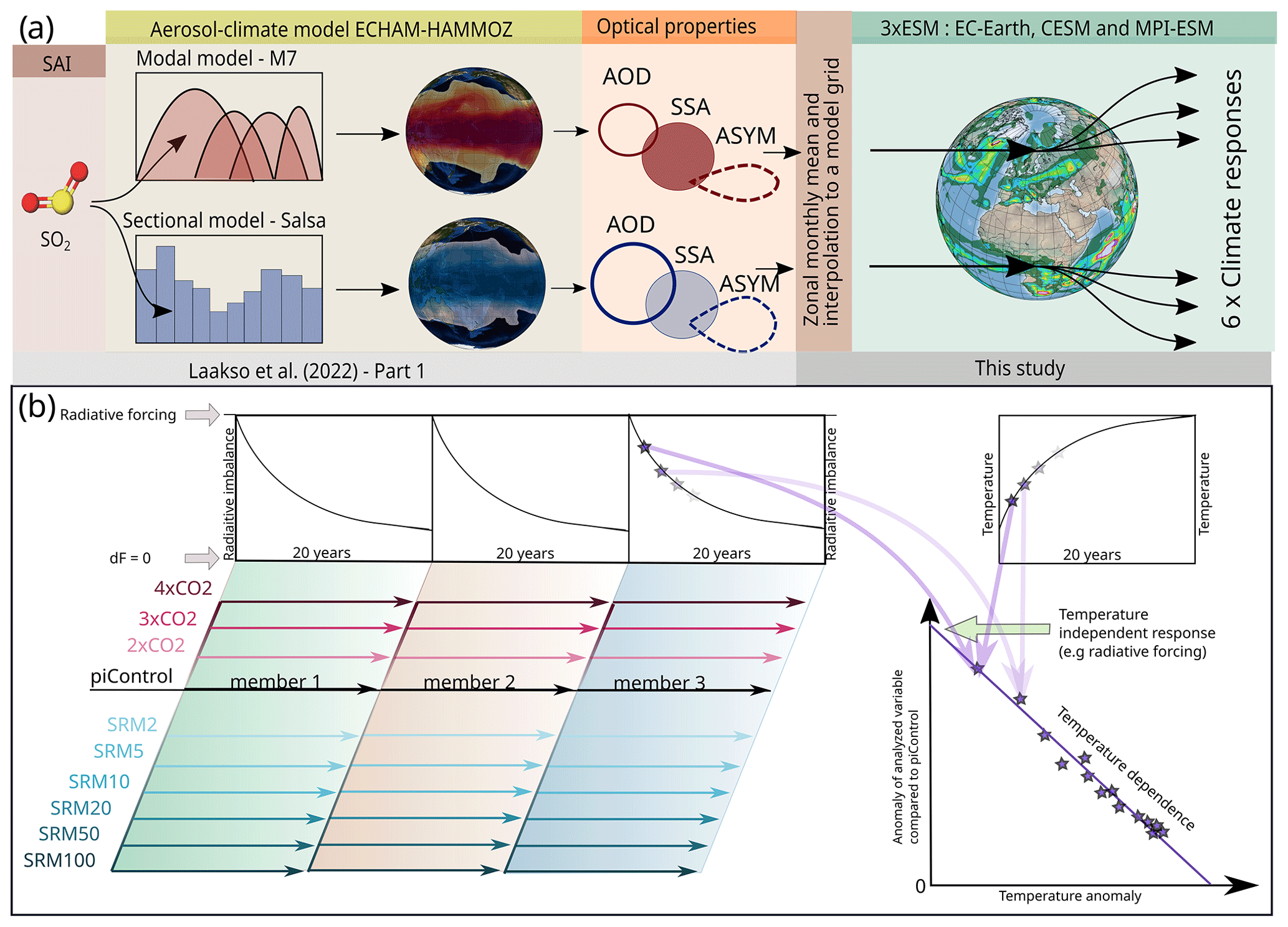
Figure 1(a) A schematic of the implementation of aerosol optical properties simulated in Laakso et al. (2022) to ESMs in this study. (b) Simulated regression scenarios and using them to quantify global mean temperature-independent responses and quasi-linear dependence on global mean temperature.
2.4 Simulated scenarios
2.4.1 Stratospheric sulfur injections
In Part 1, we performed several different injection strategies with different injection rates. Here, we include only scenarios referred as Baseline in Part 1 of this study. In these Baseline injection scenarios, sulfur was injected continuously as SO2 to a band across all longitudes between the latitudes 10° N and 10° S. The injection was done vertically at 20–22 km altitude. Simulations were done for yearly injection rates of 1, 2, 5, 10, 20, 50 and 100 Tg(S) yr−1. In this study, we omitted the 1 Tg(S) yr−1 simulation because we wanted to focus on scenarios that are more climatically relevant and have a higher signal-to-noise ratio. Simulations were performed with both the SALSA and M7 aerosol modules.
2.4.2 Regression simulations
The regression simulations with ESMs were started from a pre-industrial baseline with GHG and SAI perturbations applied. For SAI, these perturbations were stratospheric aerosol fields (from simulations with 2, 5, 10, 20, 50 and 100 Tg(S) yr−1 injection rates) from SALSA and M7 produced in Part 1. In addition, regression simulations with 2×CO2, 3×CO2 and 4×CO2 abrupt forcing values were done as well as one simulation under pre-industrial conditions without any perturbation. As Richardson et al. (2016) pointed out, a regression length of less than 15 years might lead to variation in the quantified fast and feedback responses; on the other hand, a longer regression would improve statistics, but long-scale feedbacks would then play a larger role, which would lead to a slight non-linearity. We chose 20 years as the regression length; to improve the statistics, we simulated three ensemble members.
2.4.3 Radiation equilibrium simulations
In addition to regression simulations, we carried out simulations in which CO2-induced radiative imbalance was compensated for by SAI with ESMs. By using regression simulations, it was possible to quantify the radiative forcing for each SAI scenario with different injection rates and 2×CO2, 3×CO2 and 4×CO2 concentration changes in each ESM. As the radiative forcing of CO2 depends logarithmically on the concentration of CO2, a logarithmic fit can be done for radiative forcing values of 2×CO2, 3×CO2 and 4×CO2 concentrations to quantify the dependence of radiative forcing on the CO2 concentration. Based on this, in theory, we can calculated how large a certain stratospheric sulfur injection rate needs to be to compensate for the radiative forcing from a change in CO2 concentration (to maintain radiative balance). Here, we define these sulfur injection rate–CO2 concentration pairs to maintain the climate equilibrium and perform simulations with each of the three ESMs. These simulations are 60 years long, and the last 30 years of these simulations is used in the following analysis.
Table 1Simulated scenarios.
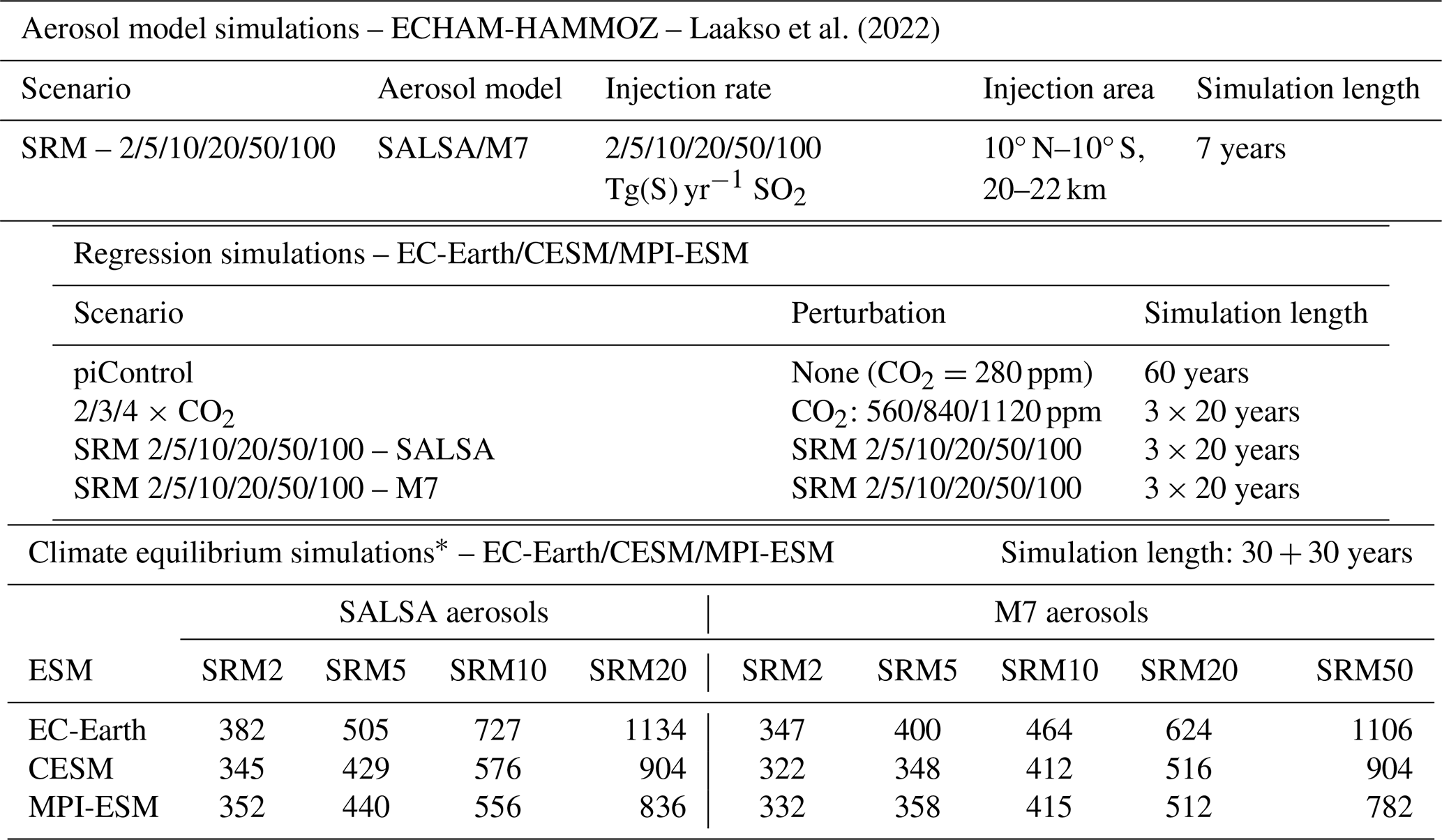
*CO2 concentration (ppm) to have presumptive radiative balance with the corresponding SAI scenario.
In Part 1, stratospheric sulfur injections were simulated with a sectional aerosol module (SALSA) and a modal aerosol module (M7). Simulated radiative forcing values are shown in Fig. 2. Simulations with both models showed that the SW radiative forcing increased sub-linearly with the injection rate, whereas the increase in LW forcing was more linear. In other respects, there was a significant difference between the model results: SW all-sky radiative forcing was 45 %–85 % higher when based on SALSA simulations than with M7, whereas LW radiative forcing was 32 %–67 % higher in M7 than in SALSA depending on the injection rate. Thus, the total radiative forcing was 88 %–154 % higher in SALSA than in M7. Details behind these differences are discussed in Laakso et al. (2022), but M7 generally produced significantly larger aerosols than SALSA. This was caused by both the treatment of the modal size distribution in M7, which prevented aerosols from having an optimal size for scattering under continuous injections, and the fact that injected sulfur tended to form new particles in SALSA instead of condensing on the existing ones, whereas M7 displayed the opposite behaviour.
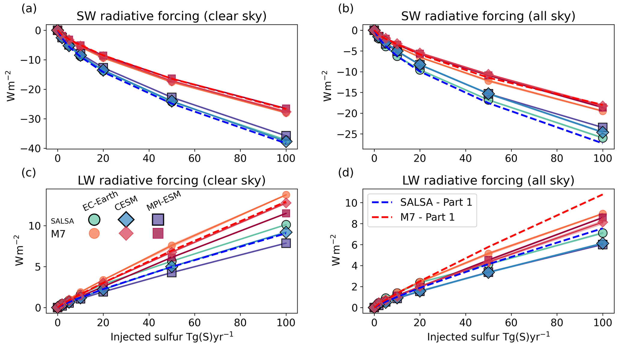
Figure 2Global mean short-wave (a) clear-sky and (b) all-sky and global mean long-wave (c) clear-sky and (d) all-sky radiative forcing as a function of injection rate. Solid lines are radiative forcing from ESM simulations with SALSA- and M7-simulated aerosols and based on regression simulations. Dashed lines shows results from Laakso et al. (2022).
To ensure that the implementation of stratospheric aerosols is done correctly, the radiative forcing simulated by each ESM is compared to the radiative forcing simulated by ECHAM-HAMMOZ in Part 1 (see Fig. 2 in this paper). When comparing these results to the radiative forcing in Part 1, it should be kept in mind that the methods for quantifying radiative forcing was different for ESM simulations compared with Part 1, as the radiative forcing of SAI scenarios in the ESMs is calculated based on Gregory plots for all-sky SW, LW and total radiative forcing of regression simulations (Gregory et al., 2004). These plots are shown in the Supplement (Figs. S1–S3). As the figures show, global mean radiation flux changes are rather linear with respect to global temperature change. From these figures, we can quantify the radiative forcing from the y intercept. In Part 1, the radiative forcing was calculated by a double radiation call with and without aerosols from simulations with fixed sea surface temperature (SST). This allowed the effects of land surface temperature adjustment and subsequent feedbacks to influence radiation. In addition, the background conditions were different: here, the radiative forcing values are calculated under pre-industrial conditions, whereas simulations were done under the year 2005 conditions in Part 1. Moreover, radiative properties were not identical between ESM simulations and ECHAM-HAMMOZ simulations, as the zonal monthly mean of radiative properties of stratospheric aerosols was used in ESM simulations, whereas radiative properties were calculated online in ECHAM-HAMMOZ.
Figure 2 shows the clear-sky and all-sky SW and LW radiative forcing of SAI as a function of injection rate in MPI-ESM, EC-Earth and CESM. Although the radiative forcing values derived from the ESMs and simulations in Part 1 are not exactly the same measure, they can be used to see if the implementation of the stratospheric aerosols to ESMs was done correctly. The comparison shows the difference in the total radiative forcing between the ESMs and Part 1 results (−27 % to 35 %). Despite these differences, this comparison provides assurance that the implementation of the radiative properties has been carried out correctly, especially as radiative forcing values between the ESM simulations are in good agreement. Particularly in the case of clear-sky SW forcing, the models exhibit similarities, as expected, due to the similarity in incoming solar radiation, which remains unaltered by clouds. LW radiation and SW all-sky radiation forcing values are more dependent on the background conditions and some unique features of each model, e.g. clouds, regional distribution of temperature and emitted LW radiation, and ice sheets and surface albedo, causing some difference in results between ESMs. In summary, this indicates that the total radiative forcing of SAI can differ slightly among ESMs, despite them having identical radiative properties for the stratospheric aerosols.
In this section, we begin by employing regression analyses on simulations to estimate the temperature changes in simulated SAI scenarios, based on the effective climate sensitivity. We then proceed to quantify the fast precipitation response and the radiative forcing associated with simulated SAI and CO2 perturbations. These metrics allow us to estimate the extent of CO2 radiative forcing that each simulated SAI scenario could offset. Given the assumption that there should be no change in global mean temperature, the quantified fast precipitation responses can then be utilized to estimate changes in global mean precipitation in scenarios in which the radiative forcing values of SAI and CO2 are balanced. Lastly, we conduct climate equilibrium simulations for various SAI injection rates and their corresponding CO2 concentrations. These simulations are utilized to examine how estimated precipitation changes, based on the fast precipitation responses, differ from the actual simulated values and to analyse regional responses.
4.1 Quantifying fast and slow responses from regression simulations
4.1.1 Global mean temperature change under SAI
From regression simulations and the regression line for total radiative flux change (Fig. S3), it is possible to estimate how much the global mean temperature will have changed when it does settle into the new radiative balance after SAI is started (considering a fixed injection amount per year). This measure is called the “effective climate sensitivity” (this term is generally used for the corresponding temperature change for the 2×CO2 experiment). It does not consider some of the longer-term non-linear climate feedbacks that are accounted for in the equilibrium climate sensitivity. Nevertheless, the effective climate sensitivity is a good estimate of temperature changes without simulations spanning over thousands of years, which would be required to quantify the equilibrium climate sensitivity (Gregory et al., 2004). However, it should be kept in mind that temperature change estimates at equilibrium are underestimated if quantified from the effective climate sensitivity; this is especially true here, as we define the slope from only the first 20 years after the induced forcing.
In addition to the magnitude of radiative forcing, the temperature change is influenced by feedback mechanisms, which vary in magnitude for each of the ESMs. Some of the simulated scenarios were quite extreme and led to over 6 K change in the global mean temperature during our 20-year simulation period. Naturally, this has a large impact on feedbacks, especially those that are not always linearly dependent on temperature, e.g. cloud and albedo feedbacks. Thus, the dependence of radiative flux change on the global mean temperature is not totally linear.
Figure 3a shows the global mean temperature change as a function of the SAI injection rate in MPI-ESM, CESM and EC-Earth based on the effective climate sensitivity. As the figure shows, simulations in which SALSA-modelled aerosols are implemented lead to significantly larger global mean cooling values compared with M7 aerosols. As expected, larger radiative forcing values from SALSA-simulated aerosols translate to a larger global mean temperature change. In addition, based on M7, the cooling impact decreases much faster as a function of injection rate than if aerosols are simulated with SALSA, which is also the same pattern that we saw for the global mean radiative forcing (Fig. 2). Moreover, there are differences in the results between ESMs. The cooling value is largest in EC-Earth compared with other ESMs with the same aerosols. In EC-Earth, both the total radiative forcing and the effective climate sensitivity parameter were slightly larger (more negative) compared with the other models. Overall, the variation in results between the ESMs was smaller compared with the difference originating from using different aerosol microphysics (M7 vs. SALSA).
In Fig. 3a CESM shows the lowest temperature change in SAI simulations, although, based on 4×CO2 simulation in Zelinka et al. (2020), the CESM climate sensitivity was higher compared with EC-Earth and MPI-ESM. This is partly explained by the different responses to the SAI and change in CO2 concentration: in CESM, the climate sensitivity parameter (i.e. the slope of the TOA radiative forcing as a function of temperature change) seems to be lower under CO2-induced warming than when negative radiative forcing was induced with SAI (see Fig. S3). This means that CO2-induced forcing causes a larger temperature change than corresponding forcing induced by SAI. However, based on the 4×CO2 simulations in this study, the temperature change at equilibrium based on the regressed line is 7.97, 7.80 and 5.66 K for EC-Earth, CESM and MPI-ESM, respectively, while the corresponding values were 8.2, 10.3 and 5.96 K (MPI-ESM-HR) in Zelinka et al. (2020). Note that the climate sensitivities reported in Zelinka et al. (2020) are x-intercept values from the Gregory plots for 4×CO2 simulations divided by 2. In this study, the regression line was fitted based on the first 20 years after induced forcing, whereas Zelinka et al. (2020) quantified it from 150 years. In Fig. S4, we used CMIP6 data from the 4×CO2 experiment of EC-Earth, CESM and MPI-ESM and showed how the slope of the radiation vs. temperature change regression line depends on the number of years used to make the fit and to calculate the climate sensitivity. As this figure shows, the slope becomes smaller and the effective climate sensitivity becomes larger if a larger number of years is used. The magnitude of this change in the climate sensitivity parameter is different between models. While the temperature change at equilibrium quantified from 4×CO2 scenario in EC-Earth and MPI-ESM increases from 6.75 to 8.41 and from 5.78 to 6.48 K, respectively, if 150 years are taken into account instead of 20, the temperature change increases from 8.35 to 11.71 K in CESM. Thus, when the effective climate sensitivity is calculated based on 150-year simulations, the sensitivity appears higher in the CESM model compared with the other two ESMs. However, this difference is not as pronounced when using 20-year simulations. This characteristic in the CESM results was discussed in Bjordal et al. (2020). It was identified that the increased sensitivity is due to a negative feedback mechanism that involves a reduction in the ice content within clouds in a warming climate. This feedback mechanism becomes less substantial when the climate has warmed sufficiently.
Figure 3a illustrates the divergent temperature change response observed in the MPI-ESM simulation when injected with a rate of 100 Tg(S) yr−1 using SALSA-simulated aerosols. This divergence is likely attributed to the non-linear response of short-wave (SW) clouds, as shown in the Supplement (see Fig. S5). Notably, this non-linearity becomes apparent when the climate has cooled by over 4 K in the MPI-ESM simulations.
The aforementioned observations emphasize that climate sensitivity is an idealized metric contingent on the time frame considered. It is also difficult to generalize the use of climate sensitivity, for example, in estimating the subsequent temperature change from multiple forcing agents. As demonstrated later in our analysis, it proves challenging to estimate potential outcomes regarding temperature changes via the simple summation of radiative forcing from both CO2 and SAI. From a broader perspective, arranging climate models in an order based on their level of warming according to a climate sensitivity defined over 150 years appears somewhat arbitrary. This order might change if some other time period to define climate sensitivity is considered.
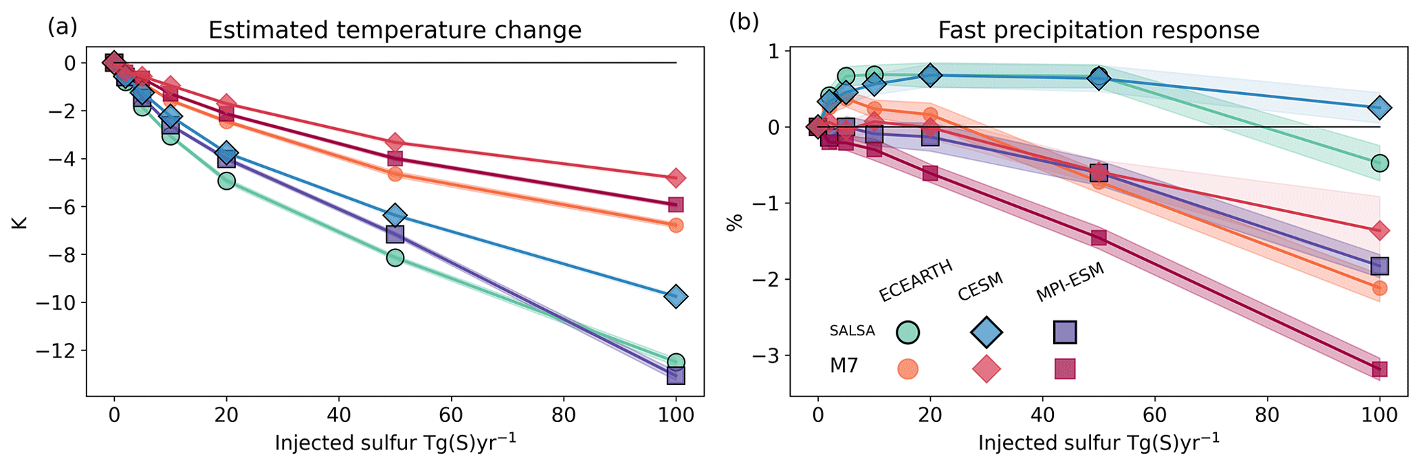
Figure 3(a) Estimated temperature changes based on the effective climate sensitivity parameter and (b) fast precipitation response as a function of sulfur injection rate based on different models. The shaded area shows the standard error of intercepts of linear fits.
4.1.2 Fast precipitation response under different injection rates
Next, we quantify the fast (temperature-independent) precipitation response under SAI and how this depends on the ESM, the aerosol microphysical model used in Part 1 and the injection rate. This is an important quantity because it indicates, for example, the imperfect cancellation of LW radiative forcing from CO2. Similarly, as for radiative forcing, the fast precipitation change can be defined from regression simulations by regressing precipitation against the global mean temperature (see Fig. S6). Fast precipitation change is then given by the y intercept. Figure 3b shows the fast precipitation response in each simulation as function of injection rate. For some simulations with small injection rates, the response is small compared with the error bars (shaded area in the figure). In general, the fast precipitation response is more positive in simulations where SALSA aerosols are used compared with those with M7 aerosols in corresponding ESM simulations, and the differences between aerosol models become more pronounced with higher injection rates. These differences among aerosol model results are even more apparent when the fast precipitation response is presented as a function of radiative forcing. For SALSA aerosols, a lower injection rate can achieve the same level of radiative forcing as M7, resulting in more significant differences in fast precipitation responses (see Fig. S7a). In addition, the fast precipitation response is non-linear as a function of both injection rate and radiative forcing. However, the standard deviation of the simulated fast precipitation response between model combinations is rather linear with respect to the injection rate and the simulated radiative forcing (see Fig. S8). This means that the differences in the simulated fast precipitation response between models become larger with larger injections.
In simulations with SALSA aerosols in EC-Earth and CESM, the fast precipitation is positive for all simulated injection rates except for 100 Tg(S) yr−1 in EC-Earth. With M7 aerosol in EC-Earth and CESM, the fast precipitation response is slightly positive or small if 20 Tg(S) yr−1 or less is injected but negative with 50 or 100 Tg(S) yr−1 injection rates. Results in MPI-ESM differ from CESM and EC-Earth results. In MPI-ESM, the fast precipitation response is small (<0.13 % of the global mean precipitation) with SALSA aerosols with an injection rate lower than 20 Tg(S) yr−1. However, at injection rates of 50 Tg(S) yr−1 and 100 Tg(S) yr−1 simulated with MPI-ESM-SALSA, global precipitation was reduced by −0.6 % and −1.83 %, respectively. The fast precipitation response in MPI-ESM–M7 simulations was also much more negative than in CESM–M7 and EC-Earth–M7 simulations. Overall, the quantified fast precipitation response due to the SAI varied between a 0.69 % increase in global mean precipitation and a −3.19 % reduction in precipitation depending on the injection rate and ESM–aerosol model combination. Based on the average hydrological sensitivity in our simulations (Fig. S6), which was 2.46 % K−1 (σ=0.28 % K−1), the range between the maximum and minimum fast precipitation responses corresponds to a global mean precipitation change associated with a temperature variation of 1.6 K.
Fast precipitation changes as a function of injection rate can be understood based on the absorbed radiation. As forcing (change in CO2 concentration or added aerosols) is induced, it changes the radiation absorbed by the atmosphere; for example, in the case of a higher CO2 concentration, more LW radiation is absorbed. Aerosols also absorb LW radiation; however, as aerosols in the stratosphere reflect solar radiation back to space, there is less radiation to be absorbed by the background atmosphere under the SAI aerosol layer. Figure 4a shows the net absorption immediately after forcing is induced (i.e. absorption part of radiative forcing) vs. fast precipitation responses in each simulated scenario. As the figure shows, the fast precipitation response and change in absorbed radiation are fairly linearly dependent, as also shown by Samset et al. (2016) and Laakso et al. (2020). This relation was quantified for each model separately, even though there are not large differences between models. We can use this quantity to calculate the individual contribution of SW and LW radiation change to fast precipitation change. This is shown by the dashed and dot-dash lines in Fig. 4b, c and d for individual ESMs and by using M7 and SALSA aerosols. As less SW radiation is absorbed, the impact on fast precipitation change is positive, whereas increased LW absorption leads to a reduced hydrological cycle. The total impact (calculated based on absorbed radiation) is shown as solid lines in Fig. 4, while the markers show actual quantified fast precipitation. As the figure shows, fast precipitation change (markers) and precipitation change, calculated from absorbed radiation, are in good agreement; thus, we can be confident that separate examination of absorbed SW and LW radiation can be used to understand the modelled fast precipitation responses.
Regardless of the model used, a common feature of all simulated fast precipitation responses is that the derivative of the fast precipitation response as a function of injection rate decreases with larger injection. In other words, the fast precipitation response as a function of injection rate is concave downwards. For some model combinations (EC-Earth–SALSA, CESM–SALSA and EC-Earth–M7), this can be seen as a positive fast precipitation response with a lower injection rate, whereas fast precipitation change is negative with larger injections. For other model combinations (CESM–M7, MPI-ESM–SALSA and MPI-ESM–M7), the fast precipitation change is negligible or rather small with 2–20 Tg(S) yr−1 injection rates, but there is a −0.6 %–3.19 % reduction in precipitation with larger injection rates. This can be understood in terms of the radiative response seen in absorbed radiation. As mentioned earlier, the impact on SW radiation causes an enhancement of the fast precipitation response, but the SW radiative forcing saturates as a function of injection rate. However, when it comes to long-wave (LW) radiation, which exerts a diminishing influence on fast precipitation, the relationship between radiative forcing and the rate of injection tends to be more linear. This means that, when considering the net impact of these two components, the significance of the LW radiation impact over the SW radiation becomes larger with a larger injection rate. This turns a positive fast precipitation response into a smaller or negative one or turns a negative fast precipitation response even more negative.
The overall precipitation response is influenced by additional factors, such as changes in temperature and fast precipitation adjustments caused by other forcing agents. For example, when SAI measures are employed to counterbalance the radiative forcing caused by increased GHGs and compensate for warming, there is an observed decrease in the hydrological cycle, mainly due to the fast precipitation response of GHGs (Laakso et al., 2020). These results show that SAI either reduces or intensifies this decrease depending on the injection rate or models used for simulations. This is studied in the next section.
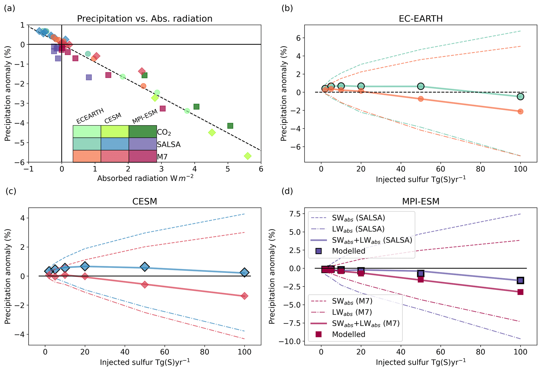
Figure 4(a) Regression of the fast precipitation response vs. atmospheric absorption and (b–d) the precipitation anomaly as a function of injection rate in EC-Earth, CESM and MPI-ESM, respectively. Markers are quantified from regression simulations by regressing precipitation against temperature, while lines are calculated from atmospheric absorption based on the relation in panel (a). The dashed line is precipitation change caused by SW absorption, the dot-dash line is based on LW absorption, the solid line is the sum of the SW and LW components, and markers are modelled fast precipitation responses from regression simulations.
4.1.3 Estimated precipitation change in climate where CO2-induced radiative forcing is compensated for by SAI
In theory, if CO2-induced radiative forcing was compensated for by SAI, the climate equilibrium should remain and there should be no change in the global mean temperature. This is not completely the case as shown, for example, by Virgin and Fletcher (2022) (and as we will see later), but we assume this right now. In this case, in which induced radiative forcing values are cancelling each other out and there is no global mean temperature change, the global mean precipitation change can be calculated by taking a sum of the fast precipitation responses of induced forcing (Laakso et al., 2020). In this case, this equates to the sum of the fast precipitation changes caused by SAI and those caused by CO2 concentration increases.
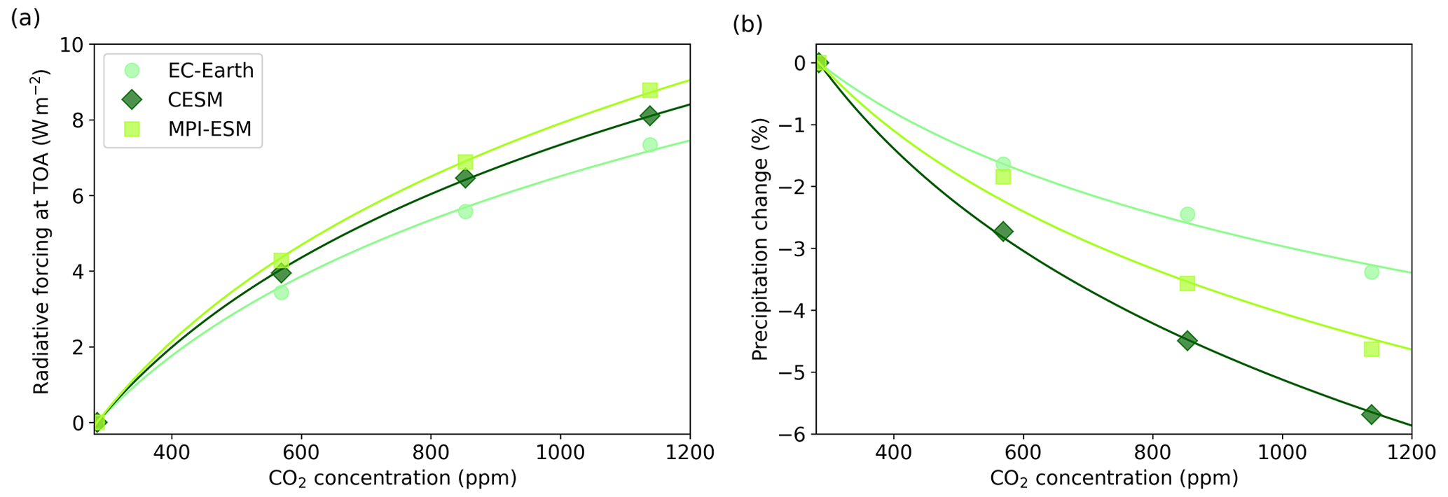
Figure 5(a) Radiative forcing at the top of the atmosphere and (b) fast precipitation response as a function of the atmospheric CO2 concentration based on the logarithmic fit for results from the piControl, 2×CO2, 3×CO2 and 4×CO2 scenarios.
First, we need to calculate the extent to which each simulated SAI experiment can compensate for changes in the CO2 concentration. We conducted four regression simulations with varying CO2 concentrations: pre-industrial, 2×CO2, 3×CO2 and 4×CO2. Using these simulations, we calculated the radiative forcing for each scenario. As we know that the radiative forcing induced by CO2 depends logarithmically on the atmospheric concentration of CO2, we used a logarithmic fit to determine the radiative forcing for each of the four simulated values (see Fig. 5). This function provides the radiative forcing for a particular CO2 concentration for each of the three ESMs. By utilizing this function and the radiative forcing for each SAI simulation, we can determine the specific CO2 concentrations for each SAI experiment at which there would be climate equilibrium. Table 1 and Fig. 6a display these CO2 concentrations.
We can now also reverse the aforementioned question and ask how large a sulfur injection has to be to offset the radiative forcing resulting from a certain increase in the atmospheric CO2 concentration. This is shown in Fig. 6a based on different model combinations (ESM–aerosol model). The total range of the estimated amount of required sulfur injection rates between model combinations is large. The greatest discrepancies are between simulations that utilize SALSA aerosols vs. those that use M7-simulated aerosol properties. As expected, due to the lower radiative forcing produced by aerosols simulated by M7, significantly higher injection rates are needed to compensate for certain CO2-induced forcing, compared with simulations that use SALSA aerosols. There were some differences between ESMs when the same aerosols were used. Regardless of the aerosols used and the considered CO2 concentration, the estimated injection rates were similar between the CESM and MPI-ESM simulations. However, in the case of EC-Earth, notably less sulfur was needed. For instance, to offset the radiative forcing of an 800 ppm CO2 concentration, EC-Earth simulations necessitated 30 %–40 % less sulfur annually compared with the corresponding CESM and MPI-ESM simulations.
To estimate the potential global mean precipitation changes in the previously mentioned scenarios, we assume a radiative balance that does not cause any temperature change. Similar to CO2-induced radiative forcing, the fast precipitation response as a function of the CO2 concentration is calculated through a logarithmic fit for pre-industrial, 2×CO2, 3×CO2 and 4×CO2 fast precipitation responses (see Fig. 5b). Assuming that there is no temperature change if the radiative forcing values from CO2 and SAI offset each other, we can calculate the global mean precipitation change as the sum of the fast precipitation response of CO2 from the fitted logarithmic function and the corresponding SAI experiment. Figure 6b displays the resulting global mean precipitation changes.
Estimates of precipitation changes depend substantially on different model combinations. As illustrated in Figs. 5b and S6, the fast precipitation response to a quadrupling of CO2 levels varied significantly, ranging from a decrease of 3.38 % in the EC-Earth simulations to a decrease of 5.6 % in the CESM simulations. However, the fast precipitation response to SAI accounts for differences of up to 3.5 % in the global mean precipitation, as illustrated by the fast precipitation response component in Fig. S7b. If M7 aerosols are used, models project a greater reduction in precipitation relative to the baseline than if SALSA aerosols are used with the same ESM. This is expected, as the absorption of LW radiation is greater in M7-based aerosols than in SALSA and more sulfur is required to offset CO2-induced forcing when using M7 aerosols. There is not a large difference in precipitation changes between MPI-ESM and CESM when using both M7 and SALSA aerosols, while there is a smaller decrease in precipitation in EC-Earth compared with simulations with the two other ESMs regardless of the aerosol model used. This is due to two factors in EC-Earth simulations: the smaller magnitude of the fast precipitation response to CO2 (as shown in Fig. 5b) compared with MPI-ESM and CESM, and the more positive fast precipitation response to SAI when the injection rate is adjusted to match the radiative forcing of CO2 (refer to Fig. S7b).
However, as indicated by Fig. S6, employing a simplistic approach using fast and slow responses to estimate precipitation changes may not be straightforward. Figure S6 reveals variations in the hydrological responses among three ESMs, particularly in the variation in the hydrological sensitivity (i.e. the slope in the figure) across various simulated forcing agents. Simulations using CESM and MPI-ESM suggest that the hydrological sensitivity increases with larger injections, but the range of this increase differs significantly from the sensitivity observed in simulations in which the CO2 concentration was perturbed. Conversely, in EC-Earth simulations, hydrological sensitivity ranged from 2.39 to 2.48 % K−1 in scenarios with CO2 perturbations, while the total range was 2.79–3.22 % K−1 in SAI scenarios. This discrepancy is a crucial factor to consider, especially in cases in which the forcing values induced by CO2 and SAI do not fully offset each other, but it might also have an impact when they are expected to compensate for each other.
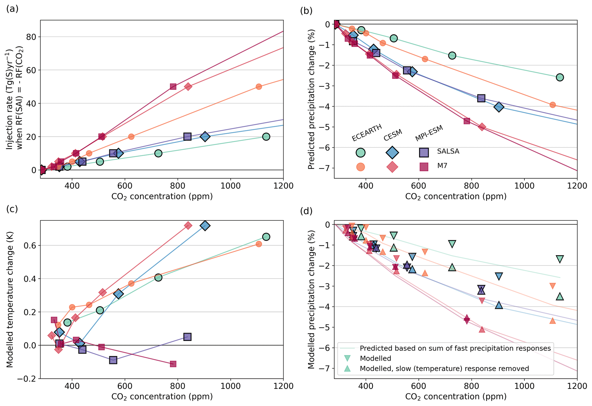
Figure 6(a) The estimated injection rate of stratospheric sulfur injections and (b) estimated precipitation change in different model combinations if the radiative forcing (RF) of the CO2 concentration is compensated for by SAI. Global mean precipitation change is calculated as the sum of the fast precipitation changes from SAI and CO2, assuming that there is no change in the global mean temperature. Based on the logarithmic relationship between radiative forcing and fast precipitation response to the CO2 concentration (as shown in Fig. 5), the CO2 concentration and the subsequent fast precipitation response can be determined from the logarithmic fit so that the radiative forcing aligns with the simulated radiative forcing for SAI. Panel (c) shows simulated changes in (a) global mean temperature and (b) precipitation under SAI–CO2 paired scenarios (as illustrated in panel a), assuming a state of climate equilibrium. In panel (d), the downward-facing triangle markers show actual simulated precipitation, whereas upward-facing triangle markers show adjusted values based on hydrological sensitivity and assuming zero global mean temperature change; the solid line shows estimated precipitation change based on fast precipitation changes (as in panel b).
4.2 Results of climate equilibrium simulations
Next, we conducted simulations in which the radiative forcing values from CO2 and SAI compensated for each other based on the SAI experiment–atmospheric CO2 concentration pairs calculated in the previous section. These simulations allowed us to observe how well our estimations of precipitation changes (Fig. 6b) held and, additionally, to simulate regional changes. The simulations were conducted under pre-industrial conditions with prescribed SAI aerosol fields and by changing CO2 concentrations to corresponding levels to maintain climate equilibrium. Another option would have been to simulate specific CO2 concentrations and scale the aerosol optical properties to match the radiative forcing of CO2. However, due to the non-linear relationship between the aerosol size distribution and optical properties of stratospheric aerosols in response to injection rates, scaling would have yielded slightly divergent outcomes compared with simulations in which intermediate injection rates were simulated using the aerosol models. Moreover, adopting the scaling approach would have resulted in the loss of specific characteristics unique to both the M7 and SALSA aerosol models.
These climate equilibrium simulations were only conducted for cases in which the CO2 concentration was below 1200 ppm. As a result, the maximum injection rate that was simulated was 20 Tg(S) yr−1 using SALSA aerosols and 50 Tg(S) yr−1 using M7 aerosols. These simulations were 60 years long, and the last 30 years was used in the analysis.
4.2.1 Global mean temperature change in climate equilibrium simulations
Figure 6c shows the global mean temperature changes in the climate equilibrium simulations as a function of the atmospheric CO2 concentration. Note that these simulations now include SAI aerosol fields and change the atmospheric CO2 concentration, which is specific for injection rates and the model (seen Table 1 and Fig. 6a). From Fig. 6c, it is clear that the assumption of no global mean temperature change only holds for MPI-ESM, while most of the CESM and EC-Earth simulations show global mean warming. The largest warming in the simulated scenarios was 0.72 K in the scenario with an injection rate of 20 Tg(S) yr−1 and a CO2 concentration of 904 ppm simulated with the CESM-SALSA model combination. Based on Fig. 6c, the primary factor influencing the extent of remaining warming is the ESM, whereas the influence of the aerosol model has a comparatively minor impact. However, in simulations conducted with the CESM and EC-Earth models, in which there is observable residual warming, the magnitude of this residual warming tends to be greater when the M7 aerosol optical properties are employed across most of the simulations. Nonetheless, the warming observed in these simulations underscores the presence of non-linearity when combining individual experiments involving CO2 and SAI. This has also been seen in earlier studies, although those studies primarily focused on reducing the solar constant and the approach to provide an initial guess for solar constant reduction (Virgin and Fletcher, 2022; Russotto and Ackerman, 2018). When applying the Gregory method to assess radiative forcing values in these scenarios, the calculated values range from 0.17 to 1.25 W m−2 in the CESM and EC-Earth simulations and are up to −0.24 W m−2 in the MPI-ESM simulations, which aligns well with the simulated temperature (see Fig. S9). However, as Fig. S9 shows, the Gregory method does not work well in this case, at least for EC-Earth and CESM, as the slope defined for individual simulations varies and there is no clear linear dependence between the total radiative flux change and global mean temperature. In general, the presence of non-linearities when combining CO2 and SAI is expected based on the findings presented in Fig. S3. The figure shows that the slopes of the fitted lines (i.e ) on the Gregory plots are, on average, 41 % lower in EC-Earth simulations and 27 % lower in CESM simulations for CO2 experiments compared with SAI experiments. However, in the case of MPI-ESM simulations, there was no significant difference. We will discuss possible physical reasons for the residual global mean warming in the CESM and EC-Earth simulations in Sect. 4.2.3.
4.2.2 Simulated global mean precipitation change in climate equilibrium simulations
As there is an increase in the global mean temperature in these simulations, the actual simulated global mean precipitation differs fundamentally from the estimated values in the previous section. In Fig. 6d, the solid lines show the estimated precipitation change using fast precipitation responses (same as Fig. 6b). Triangle markers that point down show the actual simulated precipitation in these scenarios. As global mean temperature changes were rather small in the MPI-ESM simulations, the actual simulated precipitation changes were close to the estimated values. However, as there was a slight warming in the EC-Earth and CESM simulations, the global mean precipitation is more positive than values estimated from the sum of fast precipitation responses. Hydrological sensitivity (i.e. the ratio of precipitation change to temperature change) can be used to remove the impact of global mean temperature on precipitation. Triangle markers that point up are adjusted values of simulated precipitation, generated by counteracting the impact of temperature change. Now, the adjusted values from the CESM simulations are close to the estimated ones. For EC-Earth, this adjustment corrects precipitation values in the direction of estimated values, but it results in an overadjustment for most of the simulated scenarios. It remains unclear why this temperature adjustment leads to an overestimation in the results for EC-Earth simulations. However, this could be related to the larger hydrological sensitivities for SAI compared with CO2 perturbations, as discussed in Sect. 4.1.3. Although there are discrepancies between the actual simulated values and the estimated ones, this analysis shows that estimating the total precipitation change based on the sum of the fast precipitation responses of SAI and change in CO2 concentration gives rather good results, even though there are some changes in the global mean temperature. The main conclusions also hold after analysing the actual simulations: there are large variations in the global mean precipitation between models, and larger aerosols based on M7 lead to a larger reduction in precipitation than those simulated by SALSA.
4.2.3 Regional temperature responses in the equilibrium scenarios
Figure 7 shows the zonal mean, while Fig. 8 presents the regional temperature response in the climate equilibrium simulations for selected scenarios. The regional responses for all scenarios are shown in Figs. S10 and S11. Several earlier studies have shown that compensating for GHG-induced warming with low-latitude SAI or SRM generally leads to residual warming at high latitudes and overcooling at low latitudes (e.g. Schmidt et al., 2012; Kravitz et al., 2013a; Visioni et al., 2021), unless the injections are explicitly targeted to avoid this imbalance (Kravitz et al., 2017, 2019; MacMartin et al., 2017). Laakso et al. (2022) demonstrated that the radiative forcing from SAI is primarily concentrated around the Equator for aerosols simulated using both the SALSA and M7 models. There was also significant clear-sky zonal forcing observed at the latitudes of 50° N and 50° S. However, the presence of clouds in these regions reduced the aerosol all-sky radiative forcing. Aerosol optical properties were consistently applied across all three ESMs, but variations in cloud cover and properties among the ESMs can lead to differences in the actual radiative impact of aerosols.
Here, overcooling of tropics is only seen in MPI-ESM simulations. As there was global mean warming in the CESM and EC-Earth simulations, there are fewer and smaller regions (compared with the MPI-ESM simulations) that show a negative temperature anomaly, especially within scenarios with higher atmospheric CO2 concentrations and SAI. However, in simulations using these models, the temperature gradient between low and high latitudes changes in a manner similar to that in MPI-ESM, and there are large areas where temperature change is not statistically significant, even in the higher-injection scenarios. There are also some differences in temperature patterns in the EC-Earth and CESM simulations: Arctic warming is slightly stronger in the EC-Earth simulations compared with the results of the two other models, while the CESM simulations show stronger warming over the tropical ocean and especially in stratocumulus regions. Overall, temperature changes (residual warming at high latitudes for all models and overcooling at low latitudes in MPI-ESM) are amplified with higher atmospheric CO2 concentrations and larger SAI injection rates. There is no clear distinguishable difference in regional patterns caused by the aerosol model, i.e. SALSA vs. M7 aerosols. However, estimating the impact of aerosols is not straightforward, as the atmospheric CO2 concentration is adjusted so that its global mean radiative forcing compensates for the radiative forcing of SAI. Thus, the atmospheric CO2 concentration is not the same in climate equilibrium simulations between M7- and SALSA-simulated aerosol for the same injection rate.
Regional temperature patterns provide some hints about the reason for the global mean residual warming observed in the EC-Earth and CESM simulations. Although the global mean radiative forcing of SAI compensates for the global mean radiative forcing from an increased CO2 concentration based on single forcing experiments, the zonal impacts are not uniform (see the mean total radiative flux change in the first 5 years of SRM20–SALSA simulations in Fig. S12). The gradient of solar radiation between high and low latitudes is steeper than for thermal radiation. Thus, the combination of a uniform reduction in both incoming SW and outgoing LW radiation leads to fundamentally less radiation at lower latitudes and more radiation at high latitudes, even though they would compensate for each other on average. Furthermore, concerning stratospheric aerosols, the impact on radiative forcing is more pronounced at the Equator and latitudes around 50° N and 50° S, where the aerosol concentration is large due to the atmospheric circulation (Laakso et al., 2017). Thus, radiative forcing is larger compared with the latitudes in between these regions (i.e 20–30° N and 20–30° S), and it is particularly prominent when contrasted with the impact on higher latitudes (Laakso et al., 2022). Thus it is possible that when high latitudes warm up, ice and snow start to melt and less solar radiation is reflected back into space.
On the other hand, the net radiative flux changes seen in Fig. S10 are more negative over the tropics in MPI-ESM simulations compared with the two other models. Additionally, for example, the warmer pattern in MPI-ESM simulations over the North Pacific and the cooler pattern over Alaska indicate that less warm air is transferred to Alaska and the Arctic by the North Pacific current, which might prevent the melting of Arctic sea ice. Similar patterns are observed in CESM simulations in which global mean warming is small (e.g. SRM2–SALSA/M7 and SRM10–M7). CESM simulations show warming in stratocumulus areas, which indicates changes in cloud radiative forcing. This is supported by Fig. S13, which illustrates the change in the SW radiation fluxes between the simulation with SAI and increased CO2 concentrations compared with the piControl simulation. As we can see, there is a reduction in reflected SW radiation over stratocumulus cloud areas in the CESM simulations, even though generally more radiation is reflected due to the SAI. Similar cloud adjustments have been noted in previous studies that conducted simulations to explore the linearity of the responses to SAI as well as CO2 responses (Virgin and Fletcher, 2022). CESM simulations with a higher CO2 concentration and a large SAI injection rate (e.g SRM20–SALSA and SRM50–M7; Fig. S10) show cooling in the North Atlantic that is associated with the weakening of the Atlantic Meridional Overturning Circulation, as also seen in simulations with global warming (Meehl et al., 2020; Fasullo and Richter, 2023).
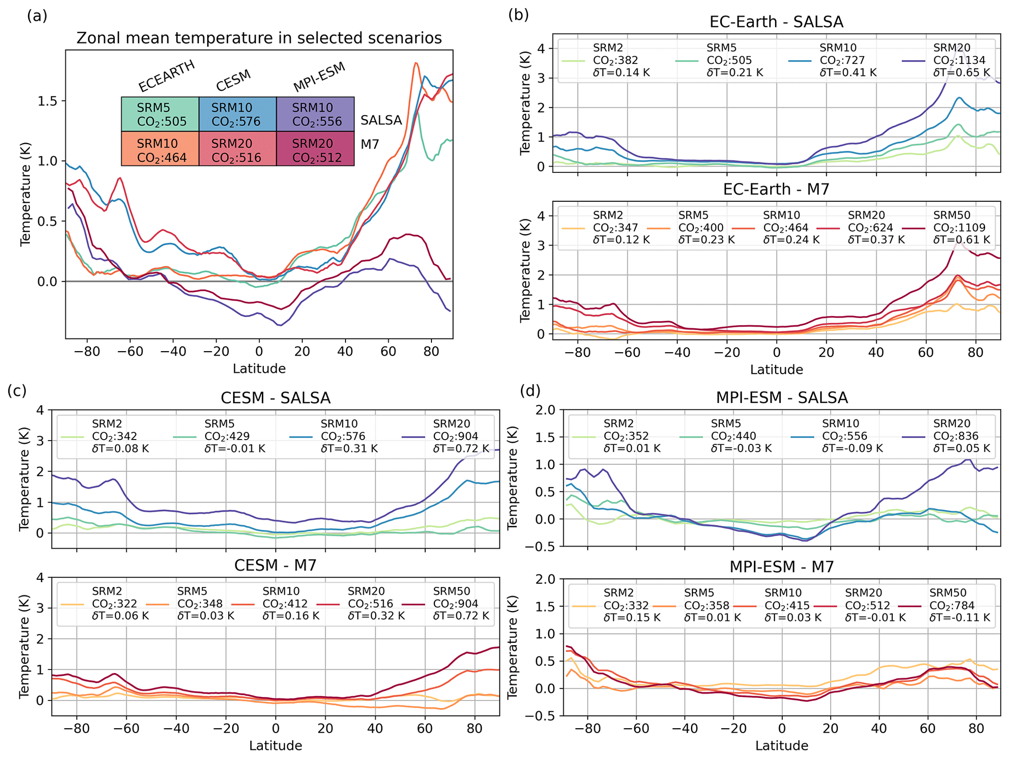
Figure 7Zonal mean temperature (a) for climate equilibrium scenarios in which the atmospheric CO2 concentration was between 464 and 576 ppm and climate equilibrium scenarios for (b) EC-Earth, (c) CESM and (d) MPI-ESM. In these simulations, the CO2 concentration was adjusted to counterbalance the radiative forcing from a specific injection rate, as determined by regression simulations. δT in the legends shows the residual global mean temperature.
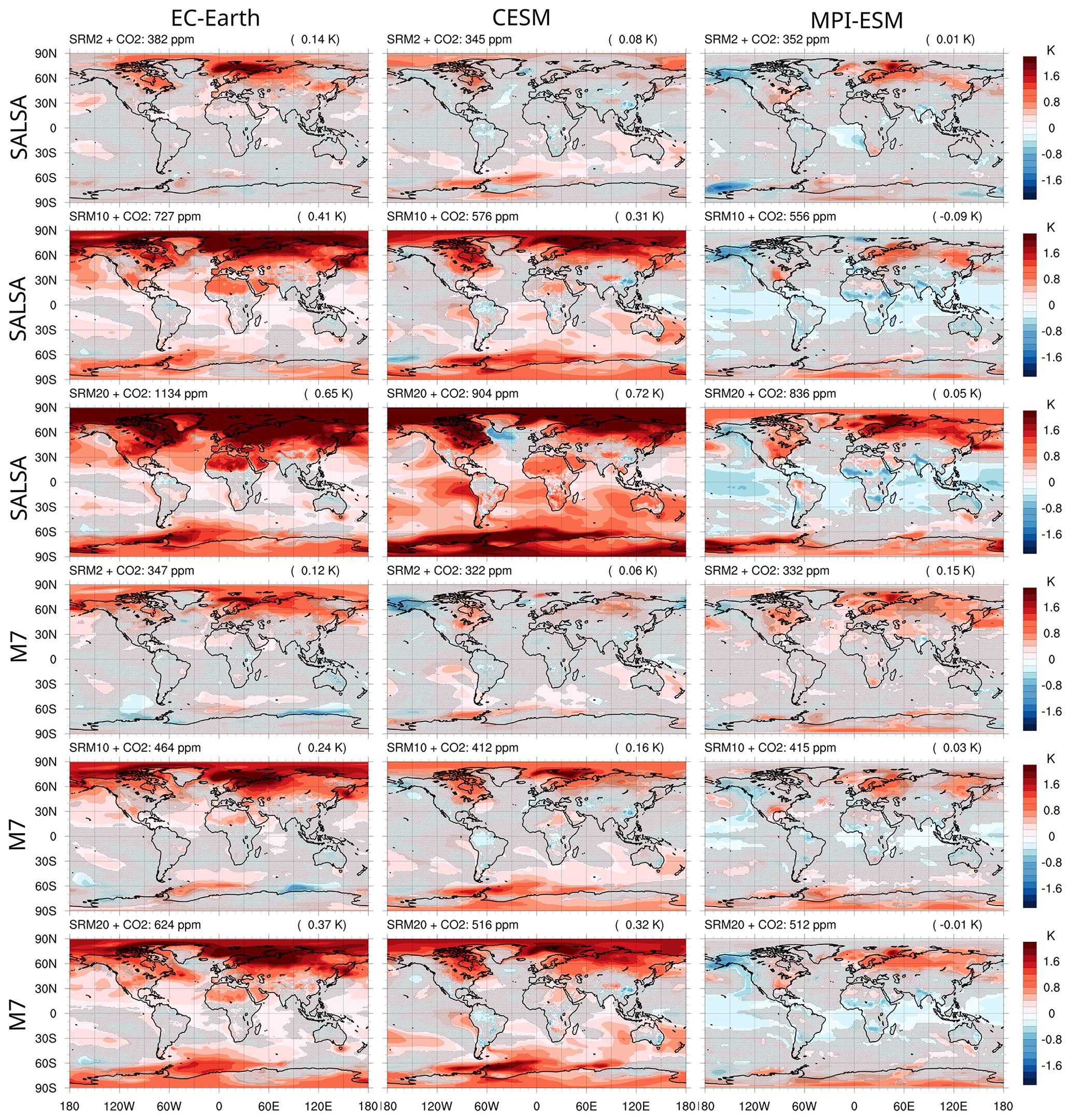
Figure 8Differences in regional temperature patterns between the climate equilibrium scenarios and piControl scenario. EC-Earth results are in the left column, CESM results are in the middle column and MPI-ESM results are in the right column. The numbers in parentheses in the upper right corner of each panel are the global mean temperature change in each scenario. Hatching indicates regions where the temperature change is not statistically significant based on the Wilcoxon signed-rank test (p value <0.05) (Wilcoxon, 1945).
4.2.4 Regional precipitation responses in the equilibrium scenarios
Figure 9 shows differences in zonal mean precipitation, while Fig. 10 shows the regional precipitation difference between the climate equilibrium simulation and piControl as an average of 30 years. In earlier sections, we focused on yearly mean values or mean periods over several years. Therefore, in this section, we focus only on averages over the years and do not analyse seasonal impacts. The regional precipitation change patterns show a shift in the Intertropical Convergence Zone (ITCZ) and a reduction in precipitation over land; however, as for the temperature impacts, the changes intensify when the CO2 concentration in the atmosphere and the SAI injection rate increase. Statistically significant precipitation changes are only observed in a minority of regions, particularly in weaker-forcing cases with a small CO2 increase and low SAI injection rates. Similar to the temperature changes discussed in the previous section, there are no significant differences in regional patterns of precipitation change when using M7 or SALSA aerosols. However, a higher CO2 concentration and larger forcing from SAI when SALSA aerosols are used lead to a more intensive impact than the corresponding injection rate using M7 aerosols.
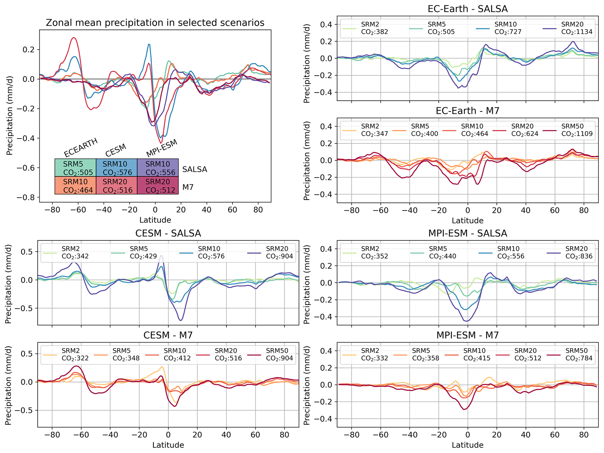
Figure 9Zonal mean precipitation (a) for climate equilibrium scenarios where the atmospheric CO2 concentrations were between 464 and 576 ppm and climate equilibrium scenarios for (b) EC-Earth, (c) CESM and (d) MPI-ESM.
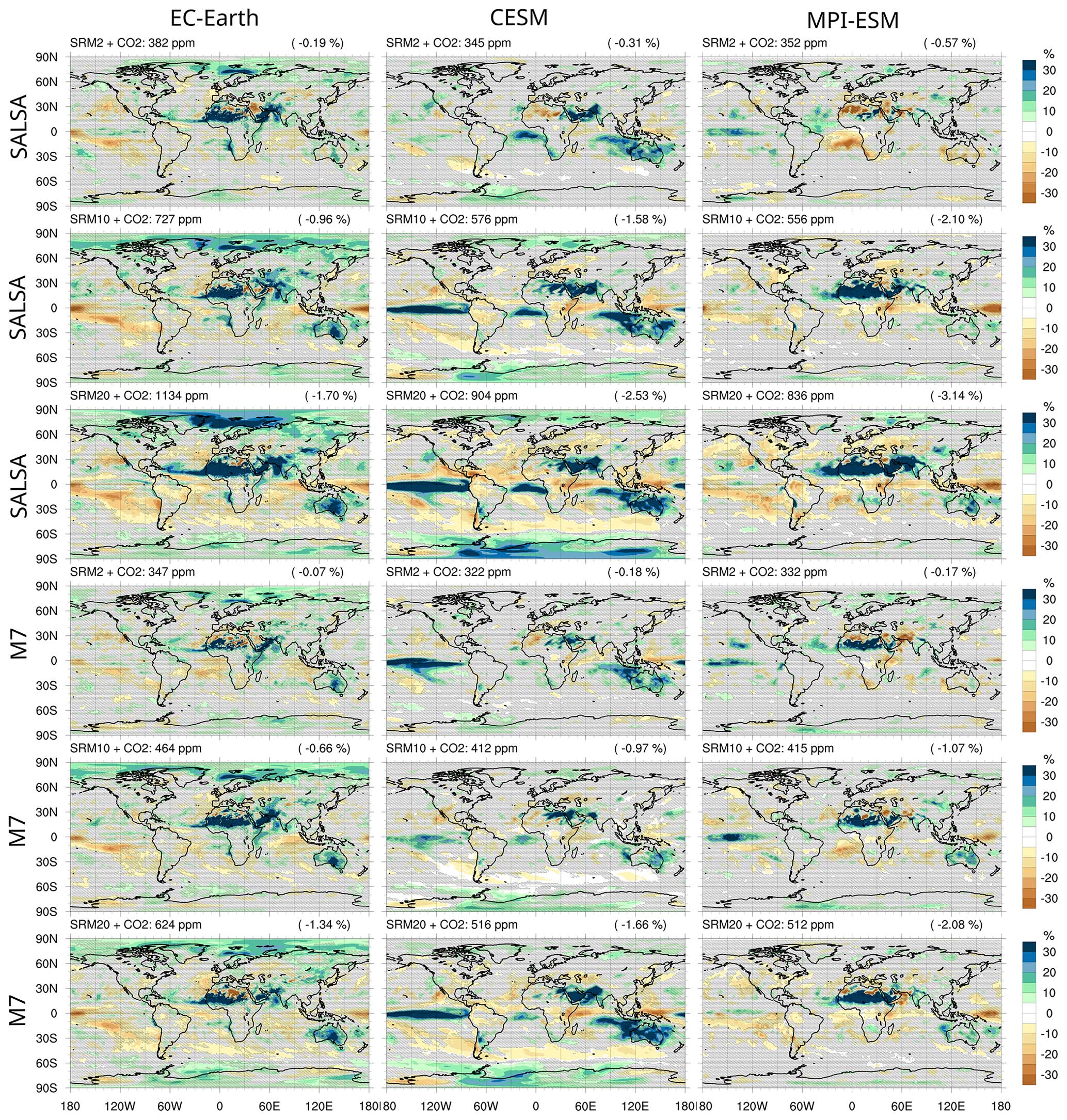
Figure 10Differences in regional precipitation patterns between the climate equilibrium scenarios and piControl scenario. EC-Earth results are in the left column, CESM results are in the middle column and MPI-ESM results are in the right column. The numbers in parentheses in the upper right corner of each panel are the global mean relative precipitation change in each scenario. Hatching indicates regions where the precipitation change is not statistically significant based on the Wilcoxon signed-rank test (p value <0.05).
There are some differences in regional patterns of precipitation between ESMs. The differences between the model responses are particularly noticeable when the CO2 concentration and SAI forcing are high. As depicted in Fig. 9, there is a decrease in precipitation over the Equator in the EC-Earth and MPI-ESM simulations, which indicates a broadening of the ITCZ. Conversely, in the CESM simulations, the ITCZ is observed to be shifting southward. EC-Earth results mostly show statistically significant increases in precipitation, whereas this is not the case in the MPI-ESM and CESM results, despite strong warming over the Arctic area in CESM. EC-Earth and MPI-ESM results indicate a relatively large increase in precipitation over the Sahel region, whereas CESM results show mostly statistically insignificant changes. According to CESM and MPI-ESM results, the tropical region in Central Africa receives less precipitation, whereas EC-Earth shows a much smaller precipitation change in that region. CESM results indicate a strong intensification of precipitation over the Equator, which is not observed in the EC-Earth or MPI-ESM results. On the other hand, there are also regions where model results agree with each other. Generally, precipitation decreases over oceans (except for the Equator in CESM results). Precipitation increases over Australia as well as in the Arabian Peninsula, Pakistan and India, but it decreases over the northern parts of South America.
In Laakso et al. (2022), we simulated SAI of different magnitudes using the sectional (SALSA) and modal (M7) aerosol schemes, and significant differences in the simulated radiative forcing values between the two aerosol models were found. In this study, we implemented the simulated radiative properties into three ESMs (EC-Earth, CESM and MPI-ESM) to study the temperature and precipitation responses under different SAI magnitudes, based on the results from the two aerosol schemes. This was done via two sets of simulations, using the aerosol optical properties from the preceding SALSA and M7 simulations for injection rates of 2–100 Tg(S) yr−1: (1) regression simulations were conducted under pre-industrial conditions with additional instantaneous forcing and (2) alleged climate equilibrium simulations were performed in which the global mean radiative forcing values of CO2 increase and SAI compensated for each other.
There was a significant difference in the responses between models. For example, the radiative forcing of SAI with an injection rate of 20 Tg(S) yr−1 varied between −3.48 and −7.16 W m−2, depending on the ESM–aerosol model combination (Fig. 2). Based on the significant differences in radiative forcing outlined in Part 1, most of the variations in radiative forcing among ESM–aerosol model combinations can be attributed to differences in the SALSA and M7 aerosol simulations. In these simulations in this study, an injection rate of 20 Tg(S) yr−1 resulted in radiative forcing values ranging from −6.75 to −7.16 W m−2 using the SALSA-simulated aerosols. In contrast, with M7 aerosols, the radiative forcing values ranged between −3.48 and −4.07 W m−2. However, an even greater variation in results was observed when examining how these differences in radiative forcing values translated into climate impacts. Based on the climate sensitivity parameter from the first 20 years of our regression simulations for a 20 Tg(S) yr−1 injection rate, the projected range for global mean temperature change spanned between −2.2 and −5.2 K. Further, this range can be subdivided into two groups: −2.2 to −2.8 K for ESM simulations in which M7 aerosols were used and −4.0 to −5.2 K for simulations based on SALSA. Simulated temperature change was smallest in the CESM simulations based on both SALSA and M7 aerosols, despite the fact that the climate sensitivity of CESM has been shown to be markedly higher compared with the other two ESMs (Zelinka et al., 2020). This discrepancy was attributed to determining the climate sensitivity parameter based on a 20-year span, rather than a 150-year period (as e.g. in Zelinka et al., 2020), as well as to differences in the responses to the SW vs. LW radiative forcing or cooling vs. warming. Except for the most extreme impact simulated in this study (simulating a 100 Tg(S) yr−1 injection rate with SALSA), the temperature change was largest in the EC-Earth simulations. This resulted from both a slightly larger climate sensitivity parameter (based on a 20-year span) and a larger simulated radiative forcing of SAI in EC-Earth compared with the other two ESMs. Overall, drawing from these results and a comparison with the climate sensitivities reported in Zelinka et al. (2020), it should be kept in mind that effective climate sensitivity is not a straightforward parameter. Its interpretation is complicated by its sensitivity to external factors, such as the type of forcing agent (which affects short-wave vs. long-wave radiation) and the length of the simulation period (e.g. 20 years vs. 100 years). Moreover, sensitivity to these external factors varies across different models.
Based on the radiative forcing quantified from regression simulations, we estimated the annual sulfur injection required to compensate for the radiative forcing of CO2 ranging from a pre-industrial concentration to 1200 ppm (see Sect. 4.1.3). The results varied significantly among different combinations of ESM–aerosol models. Based on interpolation between the simulated results, offsetting the radiative forcing from 500 ppm atmospheric CO2 concentrations required that the sulfur injection rate varied between 5 and 19 Tg(S) yr−1 between aerosol–ESM model combinations. As expected, the most significant differences arose from the choice of aerosol model used for simulations. Estimates for the required injection rate varied from 5 to 8 Tg(S) yr−1 when SALSA aerosols were employed and from 12 to 19 Tg(S) yr−1 with M7-simulated aerosols. By using quantified fast precipitation responses, we were able to estimate subsequent changes in global mean precipitation under these scenarios, assuming no alteration in the global mean temperature due to the presumed climate equilibrium. This led to a reduction in precipitation across all simulated scenarios. In the aforementioned 500 ppm atmospheric CO2 concentration and SAI scenario, the resulting global mean precipitation reduction compared with the pre-industrial climate ranged from 0.7 % to 2.4 % between different model combinations (Fig. 6). Using the same CO2 concentration within the same ESM, a larger decrease in precipitation was consistently observed when M7 aerosols were used compared with SALSA aerosols. However, when considering different ESMs, there was no distinct separation between SALSA-aerosol-based simulations, which exhibited a global mean precipitation reduction ranging from 0.7 % to 1.8 %, and M7-based simulations, which showed a reduction ranging from 1.4 % to 2.4 %. When conducting the actual simulations for these presumed climate equilibrium scenarios, we observed that the assumption of no change in global mean temperature was only valid for the MPI-ESM simulation. In contrast, in the CESM and EC-Earth simulations, there was global mean warming of up to 0.7 K in certain runs. Hence, the range of simulated precipitation reduction in the presumed climate equilibrium scenario for 500 ppm was 0.5 % to 2.0 %, which was slightly different from the earlier estimate.
We looked deeper into the global precipitation impacts caused directly by SAI, analysing its fast precipitation response. There were large differences in the fast precipitation responses between model combinations: the CESM–SALSA combination simulated positive fast precipitation changes from a 0.25 % to 0.85 % increase in global mean precipitation with injection rate levels of 2–100 Tg(S) yr−1, whereas the fast precipitation response was −0.2 % to −3.19 % in MPI-ESM–M7 (Fig. 3). However, two systematic patterns emerged in the results: (1) precipitation was always more negative in simulations in which M7 aerosols were used compared with SALSA aerosols with the corresponding injection rate; (2) all simulations with each model combination showed that the slope of the fast precipitation function with respect to the injection rate decreased with a larger injection rate. In other words, the results of all models indicate that the positive fast precipitation response turns negative if the injection rate is increased enough and that the negative precipitation change intensifies to an even greater extent when the injection rate is increased.
The fast precipitation responses can be understood based on the SAI impact on atmospheric absorption. As the global mean fast precipitation response is negatively correlated with global mean absorbed radiation, fast precipitation responses were divided into changes caused by SW and LW radiative forcing individually. The basis of SAI is that aerosol fields in the stratosphere reflect solar radiation back to space. Therefore, less SW radiation is being absorbed by the background atmosphere below the aerosol layer, leading to an increase in global mean precipitation. However, aerosols themselves also absorb LW radiation, which decreases global mean precipitation. Therefore, in the case of SAI, the fast precipitation change is a tug-of-war between these two components. From this analysis, we can understand the following systematic patterns mentioned above:
-
The fast precipitation response was consistently more negative in simulations using M7 compared with SALSA, as M7 produces fewer and larger particles than SALSA, resulting in lower SW radiative forcing (allowing more SW radiation to reach the atmosphere for absorption) but higher long-wave (LW) radiative forcing (resulting in more radiation being absorbed) compared with SALSA at the corresponding injection rate (Fig. 4).
-
As demonstrated by Laakso et al. (2022), particles become relatively larger with larger injection rates. Larger particles absorb more LW radiation, but there are relatively fewer smaller and less efficient scattering aerosols for SW radiation. Therefore, LW radiative forcing was rather linear with the injection rate, whereas SW radiative forcing saturated with larger injections. From a precipitation perspective, this means that the LW component (precipitation decrease) becomes relatively stronger against the SW component (precipitation increase) with larger injections.
Relatively minor differences in the radiative forcing of SAI in Fig. 2, in spite of the implementation of identical optical properties, and small differences in the absorption within background atmospheres across ESMs play a significantly larger role in the differing fast precipitation responses between models than one might initially expect. The decrease in absorbed SW radiation, due to the scattering from the stratospheric aerosol field, is fairly close, although with an opposing sign to the absorbed LW radiation (see Figs. S14 and S15 and Table S1 in the Supplement). As a result, the changes in total absorption were less than ±1 W m−2 for nearly all simulations, with the exception of those involving the most extreme injection rates with M7 aerosols (see Table S1 in the Supplement). In this context, even a slight variation in absorption changes due to SAI across ESMs can have a relatively large impact. For example, while the variation in LW ESMs was minimal, the reduction in SW absorption was 0.12–1.57 W m−2 smaller in simulations using MPI-ESM compared with those conducted with CESM and EC-Earth. Consequently, the total absorption in MPI-ESM simulations was greater than in the other two ESMs, particularly at higher injection rates. This led to a more pronounced negative fast precipitation response in MPI-ESM relative to the other two models. The reasons for the differences in the absorption of radiation, or radiative forcing, among ESMs are not entirely clear. However, they may be influenced by properties of the background atmosphere and surface, such as clouds, albedo, aerosols and gaseous components. Model features and simulation characteristics, like resolution, interpolation of SAI fields, and differences in radiation schemes or how these schemes are integrated with the atmospheric model, might also play a role. An in-depth analysis of these factors is beyond the scope of this study. In equilibrium simulations (see Fig. 6), variations in precipitation responses across the ESMs are also influenced by disparities in the fast precipitation response to CO2 and the radiative forcing of CO2 (Fig. 5). In these simulations, the radiative forcing of CO2 also determines the SAI injection rate, which varies for each model (Fig. 6a)
The findings presented in this study, as well as in Part 1, illustrate that variations arising from the microphysical scale and the modelling of microphysical processes can result in substantial discrepancies in the global-scale climate impacts of SAI. This highlights the significant uncertainty that microphysics introduces into our estimations of SAI impacts. Therefore, greater effort should be made to improve the representation of microphysical processes in stratospheric conditions and to understand the observed differences in results between aerosol–climate models (Quaglia et al., 2023).
The analysis presented here was largely based on the quasi-linear assumption of a relationship between near-surface temperature and radiation or global mean precipitation change in the case of an abrupt change in the forcing agent. As is generally known and is demonstrated here, this assumption does not completely hold, especially for simulations spanning decades. Even though the method is not perfect, the analysis was consistent across all of the models used here and proved to be a useful tool in analysing the factors behind simulated responses.
This study only covers continuous equatorial injection within the longitude bands examined in Laakso et al. (2022) (referred to as the Baseline scenario). In Laakso et al. (2022), we simulated various alternative injection strategies involving different magnitudes as well as temporal and spatial injection patterns. Many of these alternative scenarios were found to be more effective strategies to scatter SW radiation and absorb less LW radiation than the Baseline scenario used in this study. For instance, in the Seasonal injection scenario examined in Laakso et al. (2022), which involved seasonal changes to the injection area, the simulated SW radiative forcing at an injection rate of 20 Tg(S) yr−1 with M7 was 30 % greater than in the injection scenario examined here. However, the difference in LW radiative forcing was small between the two injection scenarios. If similar climate equilibrium simulations as those carried out with the Baseline injection strategy in this work were done with the Seasonal injection strategy, a smaller injection rate would be required. Simultaneously less LW radiation would be absorbed, and it would thus result in a smaller reduction in global mean precipitation than we saw in Fig. 6. The Seasonal injection strategy also would probably lead to a more equal compensation for temperature change across latitudes and less warming in the Arctic region in climate equilibrium-style simulations, as the forcing would be more concentrated in mid-latitudes than in the tropics compared with equatorial injections. Simulating different injection strategies with ESMs is a subject for future research.
The overall results of this study indicate that there are significant uncertainties regarding the estimated impacts of the possible deployment of SAI (e.g the coefficient of variation in the fast precipitation response below an injection rate 50 Tg(S) yr−1 was above 1.5). There are large discrepancies in the global mean responses of radiative forcing, temperature and precipitation as well as in the required amount of sulfur to achieve a certain target, depending on the aerosol and ESM used. These quantities are essential for any consideration related to solar radiation management, and their large uncertainties raise concerns about the more uncertain quantities, such as regional responses or extreme climate impacts under SAI.
These findings underscore the urgent need for further research on SAI and the development of better tools to analyse and understand the possible impacts of SAI. In its current state, our understanding of the potential consequences of SAI is insufficient to seriously consider implementing these techniques in the near future.
The model data for this paper are available online (https://doi.org/10.57707/fmi-b2share.36dce66f9e4d44d0972a411a5ab0938b, Laakso, 2024).
The supplement related to this article is available online at: https://doi.org/10.5194/esd-15-405-2024-supplement.
All authors contributed to conceptualizing the study and writing the manuscript; the writing process was managed by AL. AL performed the simulations, investigation and formal analysis. DV, UN, ST and HK provided critical feedback that shaped the analysis and the presentation of the paper.
The contact author has declared that none of the authors has any competing interests.
Publisher’s note: Copernicus Publications remains neutral with regard to jurisdictional claims made in the text, published maps, institutional affiliations, or any other geographical representation in this paper. While Copernicus Publications makes every effort to include appropriate place names, the final responsibility lies with the authors.
This research has been supported by the Tiina and Antti Herlin Foundation (grant no. 20200003).
This research has been supported by the Tiina and Antti Herlin Foundation (grant no. 20200003). Ulrike Niemeier is part of the FOR 2820 VolImpact research unit (grant no. 398006378), funded by the German Research Foundation (DFG) within the VolARC project.
This paper was edited by Michel Crucifix and reviewed by Peter Irvine and one anonymous referee.
Bjordal, J., Storelvmo, T., Alterskjær, K., and Carlsen, T.: Equilibrium climate sensitivity above 5°C plausible due to state-dependent cloud feedback, Nat. Geosci., 13, 718–721, https://doi.org/10.1038/s41561-020-00649-1, 2020. a
Danabasoglu, G., Lamarque, J.-F., Bacmeister, J., Bailey, D. A., DuVivier, A. K., Edwards, J., Emmons, L. K., Fasullo, J., Garcia, R., Gettelman, A., Hannay, C., Holland, M. M., Large, W. G., Lauritzen, P. H., Lawrence, D. M., Lenaerts, J. T. M., Lindsay, K., Lipscomb, W. H., Mills, M. J., Neale, R., Oleson, K. W., Otto-Bliesner, B., Phillips, A. S., Sacks, W., Tilmes, S., van Kampenhout, L., Vertenstein, M., Bertini, A., Dennis, J., Deser, C., Fischer, C., Fox-Kemper, B., Kay, J. E., Kinnison, D., Kushner, P. J., Larson, V. E., Long, M. C., Mickelson, S., Moore, J. K., Nienhouse, E., Polvani, L., Rasch, P. J., and Strand, W. G.: The Community Earth System Model Version 2 (CESM2), J. Adv. Model. Earth Sy., 12, e2019MS001916, https://doi.org/10.1029/2019MS001916, 2020. a, b
Döscher, R., Acosta, M., Alessandri, A., Anthoni, P., Arsouze, T., Bergman, T., Bernardello, R., Boussetta, S., Caron, L.-P., Carver, G., Castrillo, M., Catalano, F., Cvijanovic, I., Davini, P., Dekker, E., Doblas-Reyes, F. J., Docquier, D., Echevarria, P., Fladrich, U., Fuentes-Franco, R., Gröger, M., v. Hardenberg, J., Hieronymus, J., Karami, M. P., Keskinen, J.-P., Koenigk, T., Makkonen, R., Massonnet, F., Ménégoz, M., Miller, P. A., Moreno-Chamarro, E., Nieradzik, L., van Noije, T., Nolan, P., O'Donnell, D., Ollinaho, P., van den Oord, G., Ortega, P., Prims, O. T., Ramos, A., Reerink, T., Rousset, C., Ruprich-Robert, Y., Le Sager, P., Schmith, T., Schrödner, R., Serva, F., Sicardi, V., Sloth Madsen, M., Smith, B., Tian, T., Tourigny, E., Uotila, P., Vancoppenolle, M., Wang, S., Wårlind, D., Willén, U., Wyser, K., Yang, S., Yepes-Arbós, X., and Zhang, Q.: The EC-Earth3 Earth system model for the Coupled Model Intercomparison Project 6, Geosci. Model Dev., 15, 2973–3020, https://doi.org/10.5194/gmd-15-2973-2022, 2022. a, b
Fasullo, J. T. and Richter, J. H.: Dependence of strategic solar climate intervention on background scenario and model physics, Atmos. Chem. Phys., 23, 163–182, https://doi.org/10.5194/acp-23-163-2023, 2023. a
Ferraro, A. J., Highwood, E. J., and Charlton-Perez, A. J.: Weakened tropical circulation and reduced precipitation in response to geoengineering, Environ. Res. Lett., 9, 014001, https://doi.org/10.1088/1748-9326/9/1/014001, 2014. a
Gregory, J. M., Ingram, W. J., Palmer, M. A., Jones, G. S., Stott, P. A., Thorpe, R. B., Lowe, J. A., Johns, T. C., and Williams, K. D.: A new method for diagnosing radiative forcing and climate sensitivity, Geophys. Res. Lett., 31, L03205, https://doi.org/10.1029/2003GL018747, 2004. a, b
Heckendorn, P., Weisenstein, D., Fueglistaler, S., Luo, B. P., Rozanov, E., Schraner, M., Thomason, L. W., and Peter, T.: The impact of geoengineering aerosols on stratospheric temperature and ozone, Environ. Res. Lett., 4, 045108, https://doi.org/10.1088/1748-9326/4/4/045108, 2009. a
Kokkola, H., Kühn, T., Laakso, A., Bergman, T., Lehtinen, K. E. J., Mielonen, T., Arola, A., Stadtler, S., Korhonen, H., Ferrachat, S., Lohmann, U., Neubauer, D., Tegen, I., Siegenthaler-Le Drian, C., Schultz, M. G., Bey, I., Stier, P., Daskalakis, N., Heald, C. L., and Romakkaniemi, S.: SALSA2.0: The sectional aerosol module of the aerosol–chemistry–climate model ECHAM6.3.0-HAM2.3-MOZ1.0, Geosci. Model Dev., 11, 3833–3863, https://doi.org/10.5194/gmd-11-3833-2018, 2018. a, b
Koll, D. D. B. and Cronin, T. W.: Earth's outgoing longwave radiation linear due to H2O greenhouse effect, P. Natl. Acad. Sci. USA, 115, 10293–10298, https://doi.org/10.1073/pnas.1809868115, 2018. a
Kravitz, B., Caldeira, K., Boucher, O., Robock, A., Rasch, P. J., Alterskjær, K., Karam, D. B., Cole, J. N. S., Curry, C. L., Haywood, J. M., Irvine, P. J., Ji, D., Jones, A., Kristjánsson, J. E., Lunt, D. J., Moore, J. C., Niemeier, U., Schmidt, H., Schulz, M., Singh, B., Tilmes, S., Watanabe, S., Yang, S., and Yoon, J.-H.: Climate model response from the Geoengineering Model Intercomparison Project (GeoMIP), J. Geophys. Res.-Atmos., 118, 8320–8332, https://doi.org/10.1002/jgrd.50646, 2013a. a
Kravitz, B., Rasch, P. J., Forster, P. M., Andrews, T., Cole, J. N. S., Irvine, P. J., Ji, D., Kristjánsson, J. E., Moore, J. C., Muri, H., Niemeier, U., Robock, A., Singh, B., Tilmes, S., Watanabe, S., and Yoon, J.-H.: An energetic perspective on hydrological cycle changes in the Geoengineering Model Intercomparison Project, J. Geophys. Res.-Atmos., 118, 13087–13102, https://doi.org/10.1002/2013JD020502, 2013b. a, b
Kravitz, B., MacMartin, D. G., Mills, M. J., Richter, J. H., Tilmes, S., Lamarque, J.-F., Tribbia, J. J., and Vitt, F.: First Simulations of Designing Stratospheric Sulfate Aerosol Geoengineering to Meet Multiple Simultaneous Climate Objectives, J. Geophys. Res.-Atmos., 122, 12616–12634, https://doi.org/10.1002/2017JD026874, 2017. a
Kravitz, B., MacMartin, D. G., Tilmes, S., Richter, J. H., Mills, M. J., Cheng, W., Dagon, K., Glanville, A. S., Lamarque, J.-F., Simpson, I. R., Tribbia, J., and Vitt, F.: Comparing Surface and Stratospheric Impacts of Geoengineering With Different SO2 Injection Strategies, J. Geophys. Res.-Atmos., 124, 7900–7918, https://doi.org/10.1029/2019JD030329, 2019. a
Laakso, A.: Data for the manuscript “Dependency of the impacts of geoengineering on the stratospheric sulfur injection strategy – Part 2: How changes in the hydrological cycle depend on injection rates and model?”, Finnish Meteorological Institute [data set], https://doi.org/10.57707/FMI-B2SHARE.36DCE66F9E4D44D0972A411A5AB0938B, 2024. a
Laakso, A., Korhonen, H., Romakkaniemi, S., and Kokkola, H.: Radiative and climate effects of stratospheric sulfur geoengineering using seasonally varying injection areas, Atmos. Chem. Phys., 17, 6957–6974, https://doi.org/10.5194/acp-17-6957-2017, 2017. a
Laakso, A., Snyder, P. K., Liess, S., Partanen, A.-I., and Millet, D. B.: Differing precipitation response between solar radiation management and carbon dioxide removal due to fast and slow components, Earth Syst. Dynam., 11, 415–434, https://doi.org/10.5194/esd-11-415-2020, 2020. a, b, c, d, e, f, g
Laakso, A., Niemeier, U., Visioni, D., Tilmes, S., and Kokkola, H.: Dependency of the impacts of geoengineering on the stratospheric sulfur injection strategy – Part 1: Intercomparison of modal and sectional aerosol modules, Atmos. Chem. Phys., 22, 93–118, https://doi.org/10.5194/acp-22-93-2022, 2022. a, b, c, d, e, f, g, h, i, j, k, l, m, n, o, p
Liepert, B. G. and Previdi, M.: Do Models and Observations Disagree on the Rainfall Response to Global Warming?, J. Climate, 22, 3156–3166, https://doi.org/10.1175/2008JCLI2472.1, 2009. a
MacMartin, D. G., Kravitz, B., Tilmes, S., Richter, J. H., Mills, M. J., Lamarque, J.-F., Tribbia, J. J., and Vitt, F.: The Climate Response to Stratospheric Aerosol Geoengineering Can Be Tailored Using Multiple Injection Locations, J. Geophys. Res.-Atmos., 122, 12574–12590, https://doi.org/10.1002/2017JD026868, 2017. a
Mauritsen, T., Bader, J., Becker, T., Behrens, J., Bittner, M., Brokopf, R., Brovkin, V., Claussen, M., Crueger, T., Esch, M., Fast, I., Fiedler, S., Fläschner, D., Gayler, V., Giorgetta, M., Goll, D. S., Haak, H., Hagemann, S., Hedemann, C., Hohenegger, C., Ilyina, T., Jahns, T., Jimenéz-de-la Cuesta, D., Jungclaus, J., Kleinen, T., Kloster, S., Kracher, D., Kinne, S., Kleberg, D., Lasslop, G., Kornblueh, L., Marotzke, J., Matei, D., Meraner, K., Mikolajewicz, U., Modali, K., Möbis, B., Müller, W. A., Nabel, J. E. M. S., Nam, C. C. W., Notz, D., Nyawira, S.-S., Paulsen, H., Peters, K., Pincus, R., Pohlmann, H., Pongratz, J., Popp, M., Raddatz, T. J., Rast, S., Redler, R., Reick, C. H., Rohrschneider, T., Schemann, V., Schmidt, H., Schnur, R., Schulzweida, U., Six, K. D., Stein, L., Stemmler, I., Stevens, B., von Storch, J.-S., Tian, F., Voigt, A., Vrese, P., Wieners, K.-H., Wilkenskjeld, S., Winkler, A., and Roeckner, E.: Developments in the MPI-M Earth System Model version 1.2 (MPI-ESM1.2) and Its Response to Increasing CO2, J. Adv. Model. Earth Sy., 11, 998–1038, https://doi.org/10.1029/2018MS001400, 2019. a, b
Meehl, G. A., Arblaster, J. M., Bates, S., Richter, J. H., Tebaldi, C., Gettelman, A., Medeiros, B., Bacmeister, J., DeRepentigny, P., Rosenbloom, N., Shields, C., Hu, A., Teng, H., Mills, M. J., and Strand, G.: Characteristics of Future Warmer Base States in CESM2, Earth Space Sci., 7, e2020EA001296, https://doi.org/10.1029/2020EA001296, 2020. a
Myhre, G., Forster, P. M., Samset, B. H., Hodnebrog, O., Sillmann, J., Aalbergsjø, S. G., Andrews, T., Boucher, O., Faluvegi, G., Fläschner, D., Iversen, T., Kasoar, M., Kharin, V., Kirkevåg, A., Lamarque, J.-F., Olivié, D., Richardson, T. B., Shindell, D., Shine, K. P., Stjern, C. W., Takemura, T., Voulgarakis, A., and Zwiers, F.: PDRMIP: A Precipitation Driver and Response Model Intercomparison Project–Protocol and Preliminary Results, B. Am. Meteor. Soc., 98, 1185–1198, https://doi.org/10.1175/BAMS-D-16-0019.1, 2017. a
Niemeier, U. and Timmreck, C.: What is the limit of climate engineering by stratospheric injection of SO2?, Atmos. Chem. Phys., 15, 9129–9141, https://doi.org/10.5194/acp-15-9129-2015, 2015. a
Niemeier, U., Schmidt, H., and Timmreck, C.: The dependency of geoengineered sulfate aerosol on the emission strategy, Atmos. Sci. Lett., 12, 189–194, https://doi.org/10.1002/asl.304, 2011. a
Niemeier, U., Schmidt, H., Alterskjær, K., and Kristjánsson, J. E.: Solar irradiance reduction via climate engineering: Impact of different techniques on the energy balance and the hydrological cycle, J. Geophys. Res.-Atmos., 118, 11905–11917, https://doi.org/10.1002/2013JD020445, 2013. a, b, c
O'Gorman, P. A., Allan, R. P., Byrne, M. P., and Previdi, M.: Energetic Constraints on Precipitation Under Climate Change, Surv. Geophys., 33, 585–608, https://doi.org/10.1007/s10712-011-9159-6, 2012. a, b
Pierce, J. R., Weisenstein, D. K., Heckendorn, P., Peter, T., and Keith, D. W.: Efficient formation of stratospheric aerosol for climate engineering by emission of condensible vapor from aircraft, Geophys. Res. Lett., 37, L18805, https://doi.org/10.1029/2010GL043975, 2010. a
Quaglia, I., Timmreck, C., Niemeier, U., Visioni, D., Pitari, G., Brodowsky, C., Brühl, C., Dhomse, S. S., Franke, H., Laakso, A., Mann, G. W., Rozanov, E., and Sukhodolov, T.: Interactive stratospheric aerosol models' response to different amounts and altitudes of SO2 injection during the 1991 Pinatubo eruption, Atmos. Chem. Phys., 23, 921–948, https://doi.org/10.5194/acp-23-921-2023, 2023. a
Richardson, T. B., Samset, B. H., Andrews, T., Myhre, G., and Forster, P. M.: An assessment of precipitation adjustment and feedback computation methods, J. Geophys. Res.-Atmos., 121, 11,608–11,619, https://doi.org/10.1002/2016JD025625, 2016. a, b
Russotto, R. D. and Ackerman, T. P.: Changes in clouds and thermodynamics under solar geoengineering and implications for required solar reduction, Atmos. Chem. Phys., 18, 11905–11925, https://doi.org/10.5194/acp-18-11905-2018, 2018. a
Samset, B. H., Myhre, G., Forster, P. M., Hodnebrog, O., Andrews, T., Faluvegi, G., Fläschner, D., Kasoar, M., Kharin, V., Kirkevåg, A., Lamarque, J.-F., Olivié, D., Richardson, T., Shindell, D., Shine, K. P., Takemura, T., and Voulgarakis, A.: Fast and slow precipitation responses to individual climate forcers: A PDRMIP multimodel study, Geophys. Res. Lett., 43, 2782–2791, https://doi.org/10.1002/2016GL068064, 2016. a, b
Schmidt, H., Alterskjær, K., Bou Karam, D., Boucher, O., Jones, A., Kristjánsson, J. E., Niemeier, U., Schulz, M., Aaheim, A., Benduhn, F., Lawrence, M., and Timmreck, C.: Solar irradiance reduction to counteract radiative forcing from a quadrupling of CO2: climate responses simulated by four earth system models, Earth Syst. Dynam., 3, 63–78, https://doi.org/10.5194/esd-3-63-2012, 2012. a
Schultz, M. G., Stadtler, S., Schröder, S., Taraborrelli, D., Franco, B., Krefting, J., Henrot, A., Ferrachat, S., Lohmann, U., Neubauer, D., Siegenthaler-Le Drian, C., Wahl, S., Kokkola, H., Kühn, T., Rast, S., Schmidt, H., Stier, P., Kinnison, D., Tyndall, G. S., Orlando, J. J., and Wespes, C.: The chemistry–climate model ECHAM6.3-HAM2.3-MOZ1.0, Geosci. Model Dev., 11, 1695–1723, https://doi.org/10.5194/gmd-11-1695-2018, 2018. a
Seeley, J. T., Lutsko, N. J., and Keith, D. W.: Designing a Radiative Antidote to CO2, Geophys. Res. Lett., 48, e2020GL090876, https://doi.org/10.1029/2020GL090876, 2021. a
Stevens, B., Giorgetta, M., Esch, M., Mauritsen, T., Crueger, T., Rast, S., Salzmann, M., Schmidt, H., Bader, J., Block, K., Brokopf, R., Fast, I., Kinne, S., Kornblueh, L., Lohmann, U., Pincus, R., Reichler, T., and Roeckner, E.: Atmospheric component of the MPI-M Earth System Model: ECHAM6, J. Adv. Model. Earth Sy., 5, 146–172, https://doi.org/10.1002/jame.20015, 2013. a
Tegen, I., Neubauer, D., Ferrachat, S., Siegenthaler-Le Drian, C., Bey, I., Schutgens, N., Stier, P., Watson-Parris, D., Stanelle, T., Schmidt, H., Rast, S., Kokkola, H., Schultz, M., Schroeder, S., Daskalakis, N., Barthel, S., Heinold, B., and Lohmann, U.: The global aerosol–climate model ECHAM6.3–HAM2.3 – Part 1: Aerosol evaluation, Geosci. Model Dev., 12, 1643–1677, https://doi.org/10.5194/gmd-12-1643-2019, 2019. a
Tilmes, S., Fasullo, J., Lamarque, J.-F., Marsh, D. R., Mills, M., Alterskjær, K., Muri, H., Kristjánsson, J. E., Boucher, O., Schulz, M., Cole, J. N. S., Curry, C. L., Jones, A., Haywood, J., Irvine, P. J., Ji, D., Moore, J. C., Karam, D. B., Kravitz, B., Rasch, P. J., Singh, B., Yoon, J.-H., Niemeier, U., Schmidt, H., Robock, A., Yang, S., and Watanabe, S.: The hydrological impact of geoengineering in the Geoengineering Model Intercomparison Project (GeoMIP), J. Geophys. Res.-Atmos., 118, 11036–11058, https://doi.org/10.1002/jgrd.50868, 2013. a
Virgin, J. G. and Fletcher, C. G.: On the Linearity of External Forcing Response in Solar Geoengineering Experiments, Geophys. Res. Lett., 49, e2022GL100200, https://doi.org/10.1029/2022GL100200, 2022. a, b, c
Visioni, D., MacMartin, D. G., Kravitz, B., Boucher, O., Jones, A., Lurton, T., Martine, M., Mills, M. J., Nabat, P., Niemeier, U., Séférian, R., and Tilmes, S.: Identifying the sources of uncertainty in climate model simulations of solar radiation modification with the G6sulfur and G6solar Geoengineering Model Intercomparison Project (GeoMIP) simulations, Atmos. Chem. Phys., 21, 10039–10063, https://doi.org/10.5194/acp-21-10039-2021, 2021. a, b
Wilcoxon, F.: Individual Comparisons by Ranking Methods, Biometrics Bull., 1, 80–83 https://doi.org/10.2307/3001968, 1945. a
Zelinka, M. D., Myers, T. A., McCoy, D. T., Po-Chedley, S., Caldwell, P. M., Ceppi, P., Klein, S. A., and Taylor, K. E.: Causes of Higher Climate Sensitivity in CMIP6 Models, Geophys. Res. Lett., 47, e2019GL085782, https://doi.org/10.1029/2019GL085782, 2020. a, b, c, d, e, f, g, h, i
Zhang, K., O'Donnell, D., Kazil, J., Stier, P., Kinne, S., Lohmann, U., Ferrachat, S., Croft, B., Quaas, J., Wan, H., Rast, S., and Feichter, J.: The global aerosol-climate model ECHAM-HAM, version 2: sensitivity to improvements in process representations, Atmos. Chem. Phys., 12, 8911–8949, https://doi.org/10.5194/acp-12-8911-2012, 2012. a
- Abstract
- Introduction
- Models and simulations
- Summary of Part 1 and evaluating the implementation of stratospheric sulfur aerosol fields in ESMs
- Results
- Conclusions and discussion
- Data availability
- Author contributions
- Competing interests
- Disclaimer
- Acknowledgements
- Financial support
- Review statement
- References
- Supplement