the Creative Commons Attribution 4.0 License.
the Creative Commons Attribution 4.0 License.
 | 05 Mar 2024
Impact of groundwater representation on heat events in regional climate simulations over Europe
Liubov Poshyvailo-Strube
Niklas Wagner
Klaus Goergen
Carina Furusho-Percot
Carl Hartick
Stefan Kollet
The representation of groundwater is simplified in most regional climate models (RCMs), potentially leading to biases in the simulations. This study introduces a unique dataset from the regional Terrestrial Systems Modelling Platform (TSMP) driven by the Max Planck Institute Earth System Model at Low Resolution (MPI-ESM-LR) boundary conditions in the context of dynamical downscaling of global climate models (GCMs) for climate change studies. TSMP explicitly simulates full 3D soil and groundwater dynamics together with overland flow, including complete water and energy cycles from the bedrock to the top of the atmosphere. By comparing the statistics of heat events, i.e., a series of consecutive days with a near-surface temperature exceeding the 90th percentile of the reference period, from TSMP and those from GCM–RCM simulations with simplified groundwater dynamics from the COordinated Regional Climate Downscaling EXperiment (CORDEX) for the European domain, we aim to improve the understanding of how groundwater representation affects heat events in Europe.
The analysis was carried out using RCM outputs for the summer seasons of 1976–2005 relative to the reference period of 1961–1990. While our results show that TSMP simulates heat events consistently with the CORDEX ensemble, there are some systematic differences that we attribute to the more realistic representation of groundwater in TSMP. Compared to the CORDEX ensemble, TSMP simulates fewer hot days (i.e., days with a near-surface temperature exceeding the 90th percentile of the reference period) and lower interannual variability and decadal change in the number of hot days on average over Europe. TSMP systematically simulates fewer heat waves (i.e., heat events lasting 6 d or more) compared to the CORDEX ensemble; moreover, they are shorter and less intense. The Iberian Peninsula is particularly sensitive with respect to groundwater. Therefore, incorporating an explicit 3D groundwater representation in RCMs may be a key in reducing biases in simulated duration, intensity, and frequency of heat waves in Europe. The results highlight the importance of hydrological processes for the long-term regional climate simulations and provide indications of possible potential implications for climate change projections.
- Article
(19947 KB) - Full-text XML
- BibTeX
- EndNote


Over the past few decades, the number of heat waves has increased (e.g., Frich et al., 2002; Christidis et al., 2015; Zhang et al., 2020). The years 2003, 2010, 2018, 2022, and 2023 were among the hottest in Europe, characterized by record-breaking near-surface air temperatures (e.g., Stott et al., 2004; Barriopedro et al., 2011; Dirmeyer et al., 2021; Yule et al., 2023; Jiang et al., 2024; Lemus-Canovas et al., 2024). With projected climate change, the occurrence of heat waves will continue to increase (e.g., Russo et al., 2015; Hari et al., 2020; Molina et al., 2020; Masson-Delmotte et al., 2021), leading to multiple negative socio-economic impacts (e.g., Amengual et al., 2014; Yin et al., 2022).
The physical mechanisms underlying heat waves have been extensively studied (e.g., Horton et al., 2016; Liu et al., 2020; Barriopedro et al., 2023). Heat waves are triggered by strong, persistent, quasi-stationary large-scale high-pressure systems associated with atmospheric blocking events, resulting in subsiding adiabatically warmed air masses and clear skies, allowing for high insolation (Tomczyk and Bednorz, 2016; Kautz et al., 2022). The evolution of heat waves depends primarily on the synoptic weather patterns in combination with ambient soil moisture conditions, further altered by multiple land–atmosphere feedback processes (e.g., Fischer et al., 2007).
European summer heat waves were often preceded by a precipitation deficit in spring (e.g., Stegehuis et al., 2021; Hartick et al., 2021). Due to the long-term soil moisture memory effect, the lack of precipitation in early spring causes negative soil moisture anomalies in early summer and strengthens the land–atmosphere coupling (a measure of the response of the atmosphere to anomalies in the land surface state) with a lower evaporation fraction. In turn, this reduces latent cooling and amplifies summer temperatures. Note that the soil moisture memory is a phenomenon of persistence of wet or dry anomalies over a long period of time, from weeks to months, after the atmospheric conditions that caused them have passed; this allows us to preserve the hydroclimatic conditions of the preceding months (e.g., Song et al., 2019). Thus, the long-term soil moisture memory can contribute to either buffering negative droughts impacts and weakening a heat wave or, conversely, delaying drought recovery and exacerbating the occurrence of a heat wave (Erdenebat and Tomonori, 2018; Martínez-de la Torre and Miguez-Macho, 2019; Hartick et al., 2021; Dirmeyer et al., 2021). In addition to precipitation, soil moisture is strongly influenced by groundwater dynamics via vertical fluxes across the water table (capillary rise) and via horizontal fluxes through gravity-driven lateral transport within the saturated zone. Here, the water table depth dictates the intensity of shallow groundwater–soil moisture and evaporation coupling (Kollet and Maxwell, 2008).
In the context of climate impact assessments, dynamical downscaling of global climate models (GCMs) with regional climate models (RCMs) is widely used to generate regional climate change scenario information (e.g., Mearns et al., 2015; Jacob et al., 2020). RCMs have been shown to provide added value to driving GCMs by better capturing small-scale processes (Giorgi and Gutowski, 2015; Torma et al., 2015; Prein et al., 2016; Rummukainen, 2016; Iles et al., 2020), but model biases (offset during the historical period against observations) and uncertainties in climate projections still remain (Hawkins and Sutton, 2009; Sørland et al., 2018; Evin et al., 2021). In fact, many RCMs tend to overestimate duration, intensity, and frequency of heat waves (e.g., Vautard et al., 2013; Plavcová and Kyselý, 2016; Lhotka et al., 2018; Furusho-Percot et al., 2022).
The role of soil moisture in modelling heat waves is crucial (Seneviratne et al., 2006, 2010; Fischer et al., 2007), but due to the complexity of the processes involved and related high computational cost, the explicit representation of hydrological processes is oversimplified in most RCMs. Commonly applied hydrology schemes are based on 1D parameterizations in the vertical direction with runoff generation at the land surface and a gravity-driven free-drainage approach as the lower boundary condition. In such a parameterization there is no lateral subsurface flow and only the 1D Richards' equation is solved (e.g., Niu et al., 2007). RCMs with a simplified representation of hydrological processes have difficulty reliably reproducing the partitioning of land surface energy flux and, consequently, near-surface air temperatures, leading to warm biases (e.g., Barlage et al., 2021). Hydrological parameters tuning (e.g., Teuling et al., 2009; Bellprat et al., 2016) or developing new parameterizations of groundwater dynamics (e.g., Liang et al., 2003; Schlemmer et al., 2018) have been shown to improve model results. Feedback mechanisms between groundwater, land surface, and atmosphere are also often simplified in RCMs. A physically consistent description of hydrological processes in RCMs can be achieved by an explicit representation of 3D soil and groundwater hydrodynamics together with overland flow, accounting for feedback loops over the terrestrial system and complete water and energy cycles from groundwater across the land surface to the top of the atmosphere (Maxwell et al., 2007), as for instance in the Terrestrial Systems Modelling Platform (TSMP) (e.g., Shrestha et al., 2014; Gasper et al., 2014), a regional climate system model.
Keune et al. (2016) demonstrated a relationship between the representation of groundwater dynamics and near-surface air temperature for the August 2003 European heat wave from the TSMP simulation nested within the ERA-Interim reanalysis (Dee et al., 2011). In their study, the TSMP model was set up over the European domain of the COordinated Regional Climate Downscaling EXperiment (CORDEX) (e.g., Gutowski et al., 2016; Jacob et al., 2020) with two different groundwater configurations: simplified 1D free-drainage approach and 3D physics-based variably saturated groundwater dynamics. The clear impact of groundwater dynamics on the land surface water and energy balance is shown: latent heat fluxes are higher and maximum temperatures are lower, especially in areas with shallow water table depth, in the 3D configuration compared to the simplified 1D free-drainage approach. The work of Keune et al. (2016) suggests that 3D groundwater dynamics in TSMP alleviate the evolution of a single heat wave due to weaker land–atmosphere feedbacks compared to a simplified 1D free-drainage approach, at least during the investigated European heat wave of summer 2003. The ability of an explicit representation of groundwater dynamics to moderate air temperatures during a single seasonal heat wave in RCM simulations was also demonstrated in Barlage et al. (2015, 2021) and Mu et al. (2022).
Further studies were carried out to understand whether the aforementioned effects of the groundwater representation persist over longer time periods in RCM evaluation runs and how this manifests itself for heat waves over Europe. Furusho-Percot et al. (2019) show that TSMP simulations driven by the ERA-Interim reanalysis capture climate system dynamics and the succession of warm and cold seasons at the regional scale for PRUDENCE regions (Christensen and Christensen, 2007) consistent with the E-OBS observations (Cornes et al., 2018) for the investigated period of 1996–2018. Moreover, the TSMP multiannual evaluation run exhibits lower deviations of summer heat wave indices from the E-OBS observations compared to the CORDEX RCMs with a simplified representation of groundwater, which tend to simulate too persistent heat waves (Furusho-Percot et al., 2022). This particular behaviour of TSMP is attributed to its improved hydrology, which leads to a better capacity to sustain soil moisture and therefore a more reliable latent heat flux and evaporation. This leads to a decrease in the number of days with anomalously high near-surface temperatures, as well as the intensity and spatial extent of heat waves. An important question still remains: how will these findings be reflected in long-term regional climate simulations in the context of dynamical downscaling of GCMs by RCMs for climate change studies over Europe?
In this paper, we present a unique dataset from the TSMP regional climate system model driven by the Max Planck Institute Earth System Model at Low Resolution (MPI-ESM-LR) (Giorgetta et al., 2013) historical boundary conditions over the European CORDEX domain. We interrogate the statistics of the characteristics of heat events (duration, intensity, frequency) for the summer seasons of 1976–2005 relative to the reference period 1961–1990, by comparing TSMP results and those of the CORDEX RCMs with a simplified representation of groundwater driven by GCM control simulations of phase five of the Coupled Model Intercomparison Project, CMIP5 (Taylor et al., 2012). We strive to better understand the impact of 3D groundwater dynamics on simulated heat events in historical regional climate simulations and potential consequences for climate change projections. While Furusho-Percot et al. (2022) examined the statistics of heat events in the TSMP evaluation run, the long-term TSMP historical climate simulations forced by MPI-ESM-LR GCM have not been previously presented or analysed. Thus, this is the first assessment of the heat event statistics over Europe from a dynamically downscaled GCM with a fully coupled RCM that comprises an explicit representation of groundwater dynamics and two-way non-linear feedbacks from groundwater across the land surface to the top of the atmosphere.
Section 2 introduces the methods, describing the TSMP modelling platform and its set-up, the procedure for detection and analysis of heat events, and the CORDEX ensemble used for comparison with the TSMP results. In Sect. 3, we examine the new TSMP dataset driven by MPI-ESM-LR GCM for consistency with the CORDEX ensemble and present results on the impact of an explicit groundwater representation on simulated heat events in long-term regional historical climate simulations. Section 4 contains the discussion, and Sect. 5 provides the summary and overall conclusions.
2.1 The TSMP modelling platform
TSMP is a scale-consistent, highly modular, fully integrated soil–vegetation–atmosphere regional climate system model (e.g., Shrestha et al., 2014; Gasper et al., 2014). TSMP consists of three component models: the atmospheric COnsortium for Small Scale Modelling (COSMO) model version 5.01, the Community Land Model (CLM) version 3.5, and the hydrological model ParFlow version 3.2. The component models are externally coupled via the Ocean Atmosphere Sea Ice Soil (OASIS) Model Coupling Toolkit (MCT) version 3.0 (Valcke, 2013), which enables interactions between different compartments of the geoecosystem, explicitly reproducing feedbacks in the hydrological cycle from the bedrock into the atmosphere.
COSMO is a non-hydrostatic limited-area atmospheric model (Baldauf et al., 2011). COSMO is based on the primitive thermo-hydrodynamical Euler equations formulated in rotated geographical coordinates and generalized terrain-following height coordinates, which describe compressible flow in a moist atmosphere. COSMO parameterization schemes cover various physical processes, such as radiation, cloud microphysics, and deep convection. The boundary conditions for COSMO are provided by a coarse-grid model, i.e., reanalysis or GCM, whereas the lower boundary conditions (e.g., surface albedo, energy fluxes, surface temperature, surface humidity) are provided by CLM in the current TSMP configuration.
CLM is a biogeophysical model of the land surface (Oleson et al., 2004, 2008). It simulates land–atmosphere exchanges in response to atmospheric forcings. CLM consist of four components that describe biogeophysics, hydrologic cycle, biogeochemistry, and dynamic vegetation. In TSMP, CLM receives short-wave radiation, wind speeds, barometric pressure, precipitation, near-surface temperature, and specific humidity from COSMO. In turn, CLM sends infiltration and evapotranspiration fluxes of each soil layer to the ParFlow hydrological model.
ParFlow is a hydrological model that simulates variably saturated 3D subsurface hydrodynamics using a Richards equation integrated with shallow overland flow based on a kinematic wave approximation (Maxwell and Miller, 2005; Kollet and Maxwell, 2006; Kuffour et al., 2020). ParFlow allows 3D redistribution of subsurface water in a continuum approach. In the TSMP configuration used, ParFlow replaces the hydrological functionality of CLM.
The evaluation run of TSMP was performed by Furusho-Percot et al. (2019) with atmospheric forcings derived from the ERA-Interim reanalysis, which was validated by comparing temperature and precipitation with E-OBS and column water storage with the Gravity Recovery and Climate Experiment (GRACE) satellite data (Landerer et al., 2020). In the recent publication of Ma et al. (2022), the TSMP water table simulation results were used in a machine learning approach and compared to in situ water table observation anomalies over Europe; the results showed good agreement considering that the TSMP model has not been calibrated.
2.2 The TSMP simulation set-up
The TSMP simulation is conducted over the European domain according to the CORDEX simulation protocol (Gutowski et al., 2016) on a rotated latitude–longitude grid with a horizontal resolution of 0.11° (EUR-11) or about 12.5 km for the historical time period from December 1949 to the end of 2005. CLM and ParFlow are initialized with the moisture conditions on 1 December 2011, extracted from the TSMP evaluation run (Furusho-Percot et al., 2019). The COSMO configuration resembles that of the COSMO model in CLimate Mode (CCLM) (Rockel et al., 2008). COSMO extends vertically up to 22 km, divided into 50 levels. CLM has 10 soil layers with a total depth of 3 m, which coincide with the 10 top layers of ParFlow. In addition, ParFlow has five bedrock layers increasing in thickness towards the bottom of the model domain to a total depth of 57 m. The time step for ParFlow and CLM is 900 s, while for COSMO it is 75 s. The coupling time step between TSMP component models is 900 s. The TSMP output constitutes terrestrial essential climate variables with a time step of 3 hours; for details, see Poshyvailo-Strube et al. (2023). The first 10 years of TSMP simulation are discarded due to hydrodynamic spin-up.
Forcing data for COSMO are provided by the Max Planck Institute's MPI-ESM-LR r1i1p1 CMIP5 GCM with a resolution of T63L47 (Giorgetta et al., 2013). For CLM, plant functional types (PFTs) are taken from the Moderate Resolution Imaging Spectroradiometer (MODIS) land cover dataset (Friedl et al., 2002). Leaf area index, stem area index, and monthly bottom and top heights of each PFT are calculated based on the global CLM surface dataset (Oleson et al., 2008). Topography in ParFlow is represented by slopes estimated from the United States Geological Survey GTOPO30 (Daac, 2004). In this study, we improved the representation of subsurface hydrogeology in ParFlow compared to the previous studies (e.g., Furusho-Percot et al., 2019, 2022), where soil parameters were assumed to be vertically homogenous. Here, an aquifer network is added to ensure the relationship between surface and subsurface water flow (Naz et al., 2023). Static land surface input data, which includes soil colour, percentage of clay and sand, dominant land use type, dominant soil types in the top layers, dominant soil types in the bottom layers, and subsurface aquifer and bedrock bottom layers, are derived from a number of datasets, namely the Food and Agriculture Organization soil database (FAO, 1988), the pan-European River and Catchment Database (Vogt et al., 2007), International Hydrogeological map of Europe (IHME) (Duscher et al., 2015), and GLobal HYdrogeology MaPS (GLHYMPS) (Gleeson et al., 2014). The information on subsurface aquifers is derived from IHME. The bedrock geology is constructed from the IHME hydrogeological information and the lower-resolution GLHYMPS, in combination with the pan-European River and Catchment Database. The pan-European River and Catchment Database serves as a proxy for the alluvial aquifer system in ParFlow, which is assumed to lie underneath or near existing rivers.
2.3 Multi-model GCM–RCM ensemble
RCMs driven by CMIP5 GCMs control simulations (r1i1p1 ensemble members) over the European domain from the CORDEX experiment at EUR-11 horizontal resolution are used in conjunction with the coupled TSMP modelling platform to study the impact of 3D groundwater dynamics on the statistics of heat events. Note that CMIP5 GCM historical control simulations are performed under observed natural and anthropogenic forcing (e.g., Taylor et al., 2012).
Giorgetta et al. (2013)Voldoire et al. (2013)Bentsen et al. (2013)Dunne et al. (2012)Dufresne et al. (2013)Shrestha et al. (2014)Rockel et al. (2008)Pothapakula et al. (2020)Jacob and Podzun (1997)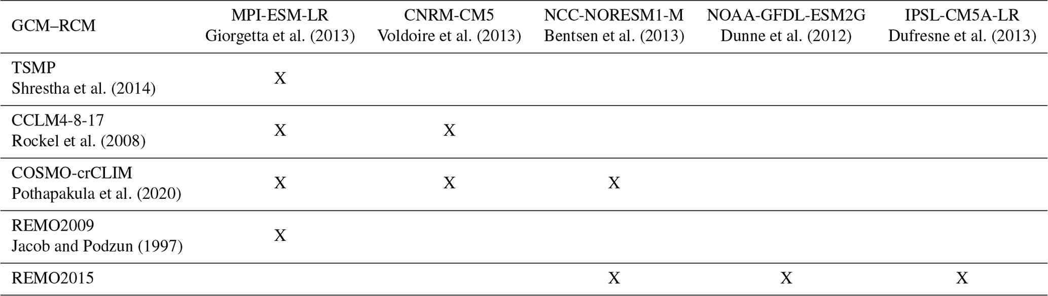
Based on data availability, this study considers the following CORDEX ensemble members identified by their institutions: CLMcom (CCLM4-8-17 driven by MPI-ESM-LR and CNRM-CM5), CLMcom-ETH (COSMO-crCLIM driven by MPI-ESM-LR, CNRM-CM5, and NCC-NorESM1-M), MPI-CSC (REMO2009 driven by MPI-ESM-LR), and GERICS (REMO2015 driven by NCC-NorESM1-M, NOAA-GFDL-ESM2G, and IPSL-CM5A-LR); see Table 1 for details. Such a multi-model GCM–RCM ensemble includes two main groups of RCMs, namely COSMO and REMO in different versions, and five different GCMs, for a total of 10 different GCM–RCM pairs. TSMP is most compatible with CCLM4-8-17, with the main differences in the COSMO lower boundary condition: in TSMP, the lower boundary condition accounts for groundwater feedbacks due to the coupling between the CLM land surface model and the ParFlow hydrological model, unlike in CCLM4-8-17, where soil processes are modelled by TERRA-ML, the soil–vegetation land surface model of COSMO (e.g., Grasselt et al., 2008; Schlemmer et al., 2018). With the exception of TSMP, the RCMs in the considered ensemble lack the closure of water and energy cycles due to simplifications of the representation of subsurface hydrodynamics.
2.4 Detection and analysis of heat events
There is no universally accepted method for detecting heat events, but the most commonly used approach is based on a percentile temperature threshold (e.g., Zhang et al., 2005, 2011; Sulikowska and Wypych, 2020). However, temperature-based diagnostics are often ambiguous or inconsistent and only partially describe heat events (Perkins and Alexander, 2013).
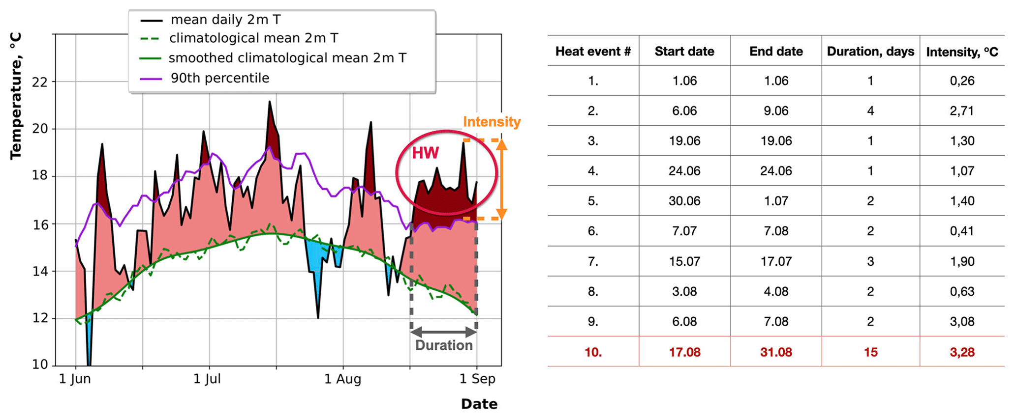
Figure 1Schematic of a summer heat wave (HW) detection. An example is given for June–July–August of 1972 for one grid element [250, 300] of the European CORDEX domain. Data taken from the TSMP simulation. The solid black line is the daily mean 2 m air temperature for the summer season of 1972. The dashed green line is the climatological daily mean 2 m air temperature for 1961–1990, and the solid green line shows its smoothing using the Butterworth filter. The solid violet line represents the 90th percentile of the daily mean 2 m air temperature calculated from a 5 d window centred on each summer calendar day of the 1961–1990 reference period. The shaded light red colour indicates days with temperatures above the climatological mean, and the shaded dark red colour highlights days with temperatures above the 90th percentile. The characteristics of the heat events (start and end dates, duration, intensity) detected during the considered summer season are also given.
In this study, we determine a day with a daily mean temperature above the local 90th percentile of the reference period as a hot day. We calculate the 90th percentile for every summer day and for each EUR-11 grid point of the European CORDEX domain from a consecutive 5 d moving window centred on that calendar day from the 30-year period between 1961 and 1990 in each RCM considered. The first occurrence of a hot day defines the beginning of a heat event. A series of hot days constitutes a heat event, highlighted in dark red in Fig. 1. A heat event is interrupted if the daily mean temperature drops below the 90th-percentile-based threshold.
A heat event can be characterized by its duration, intensity, and frequency (e.g., Horton et al., 2016). A heat event duration is the number of consecutive days over which the heat event lasts. If a heat event lasts long enough, it can be classified as a heat wave. Similar to Fischer and Schär (2010), we define a heat wave as a spell of at least 6 consecutive days with daily mean 2 m air temperatures above the local 90th percentile of the 1961–1990 reference period; see Fig. 1. The total number of hot days during the investigated period corresponds to the TG90p heat index from the joint CCl/CLIVAR/JCOMM Expert Team on Climate Change Detection and Indices (ETCCDI) (Alexander et al., 2006) and describes the number of days with TGij>TGin90, where TGij is a daily mean temperature on day i of the investigated period j, and TGin90 is the 90th percentile calculated for day i from the 30-year reference period n. Note that we consistently use the terms hot day, heat event, and heat wave throughout this article.
A heat event intensity is the maximum of the difference between the daily mean temperature and the 90th percentile of the reference period within a single heat event (e.g., Vautard et al., 2013). Intensity represents the severity of a heat event (see Fig. 1). Adopting the definition of the heat wave duration index (HWDI) from Frich et al. (2002), here we classify a heat wave as intense if its intensity is at least 5 K. In literature, there are other classifications of heat waves depending on their intensity, e.g., low intensity, severe, and extreme (Nairn and Fawcett, 2014) or weak, moderate, and intense (Lhotka and Kyselý, 2015).
The frequency of heat events of a certain type (e.g., of a certain duration or intensity) over the investigated period is the number of these heat events divided by the total number of all heat events that occurred during the period under study (e.g., Vautard et al., 2013). For example, in Fig. 1, heat events with a duration of 2 d occur four times, and the total number of all heat events is equal to 10. Therefore, the resulting frequency of 2 d heat events during that summer season is 0.4, indicating that 40 % of all heat events are 2 d in duration.
In the following we examine the impact of groundwater representation on the distribution of simulated heat events in RCMs over Europe. In particular, we investigate whether the new dataset from TSMP driven by MPI-ESM-LR is consistent with the GCM–RCM climate change scenario control runs from the CORDEX ensemble (see Table 1), and we seek to gain insight into the role of explicit groundwater representation in long-term climate simulations. We assess the statistics of the characteristics of heat events, i.e., their duration, intensity, and frequency, from daily mean 2 m air temperatures on the native EUR-11 grid. The analysis is conducted in the focus domain (Fig. 2), which covers the European continent (36–70° N, 10° W–30° E). The analysis is performed for the summer seasons of the 30-year period from 1976–2005 relative to the reference period 1961–1990 for each RCM. Note that grid elements belonging to the ocean are omitted from the analysis.
3.1 Number of hot days
We examine the impact of groundwater dynamics on the interannual variability of the occurrence of hot days during the summer seasons from 1976–2005 regarding the reference period 1961–1990 in each RCM. A comparison of the time series of the number of hot days, i.e., the TG90p index, averaged over the summer season and over the focus domain shows that the impact of an explicit representation of groundwater dynamics in RCMs varies from year to year (Fig. 3). The summer TG90p index averaged between 1976 and 2005 results in 10.95 d in the TSMP simulation and 11.64 d in the CORDEX multi-model ensemble mean (see Fig. 3). A positive linear trend in the summer TG90p index is observed in all considered RCMs, with the decadal change in the TSMP simulation being 1.53 d, while this value averaged over the CORDEX ensemble reaches 1.99 d.
The spatial distributions of the seasonal mean, variability, and decadal change in the summer TG90p index are shown in Figs. 4–6. There, the spatial patterns from RCMs driven by the same GCMs show rather similar behaviour, indicating that the climatological occurrence of summer hot days is largely controlled by the large-scale atmospheric circulation imposed by the GCM boundary conditions. TSMP produces the smoothest spatial distribution of the seasonal mean and variability of the summer TG90p index compared to the CORDEX ensemble (see standard deviations in Figs. 4, 5). The mean and interannual variability of the summer TG90p index averaged over the focus domain are also lowest in TSMP compared to the CORDEX ensemble (Tables A1 and A2 in Appendix A).
The TSMP-simulated summer TG90p index is consistent with that of the RCMs driven by MPI-ESM-LR from the CORDEX ensemble, although there are some regional differences (see Figs. 4a–d, 5a–d, 6a–d). The largest differences occur in the Iberian Peninsula PRUDENCE region, with TSMP yielding the lowest values: the mean TG90p index is equal to 10.36 d in TSMP and ranges from 12.54 to 12.75 d in the CORDEX RCMs driven by MPI-ESM-LR, variability of the TG90p index reaches 6.17 d in TSMP and ranges from 8.01 to 9.59 d in the CORDEX RCMs driven by MPI-ESM-LR, and decadal change in the TG90p index is 2.26 d in TSMP and ranges from 3.66 to 4.25 d in the CORDEX RCMs driven by MPI-ESM-LR (see Appendix A). As for the decadal change, the RCMs driven by MPI-ESM-LR show a positive trend in southern and central Europe and a negative trend in northern Europe. Note that there is no unequivocal agreement in the decadal change at the entire GCM–RCM ensemble considered, yet the decadal trend of the summer TG90p index averaged over the focus domain is positive in all models of the investigated GCM–RCM ensemble, reaching values between 1.13 and 2.71 d (see Table A3 in Appendix A).
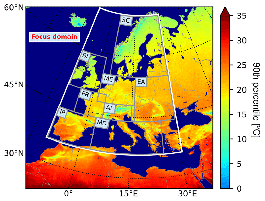
Figure 2Mean 90th percentile of 2 m air temperatures for the summer season, based on TSMP simulation from 1961 to 1990. The white box indicates a focus domain (36–70° N, 10° W–30° E) used in the analysis. PRUDENCE regions are shown with grey boxes: British Isles (BI), Iberian Peninsula (IP), France (FR), mid‐Europe (ME), Scandinavia (SC), Alps (AL), Mediterranean (MD), and eastern Europe (EA).
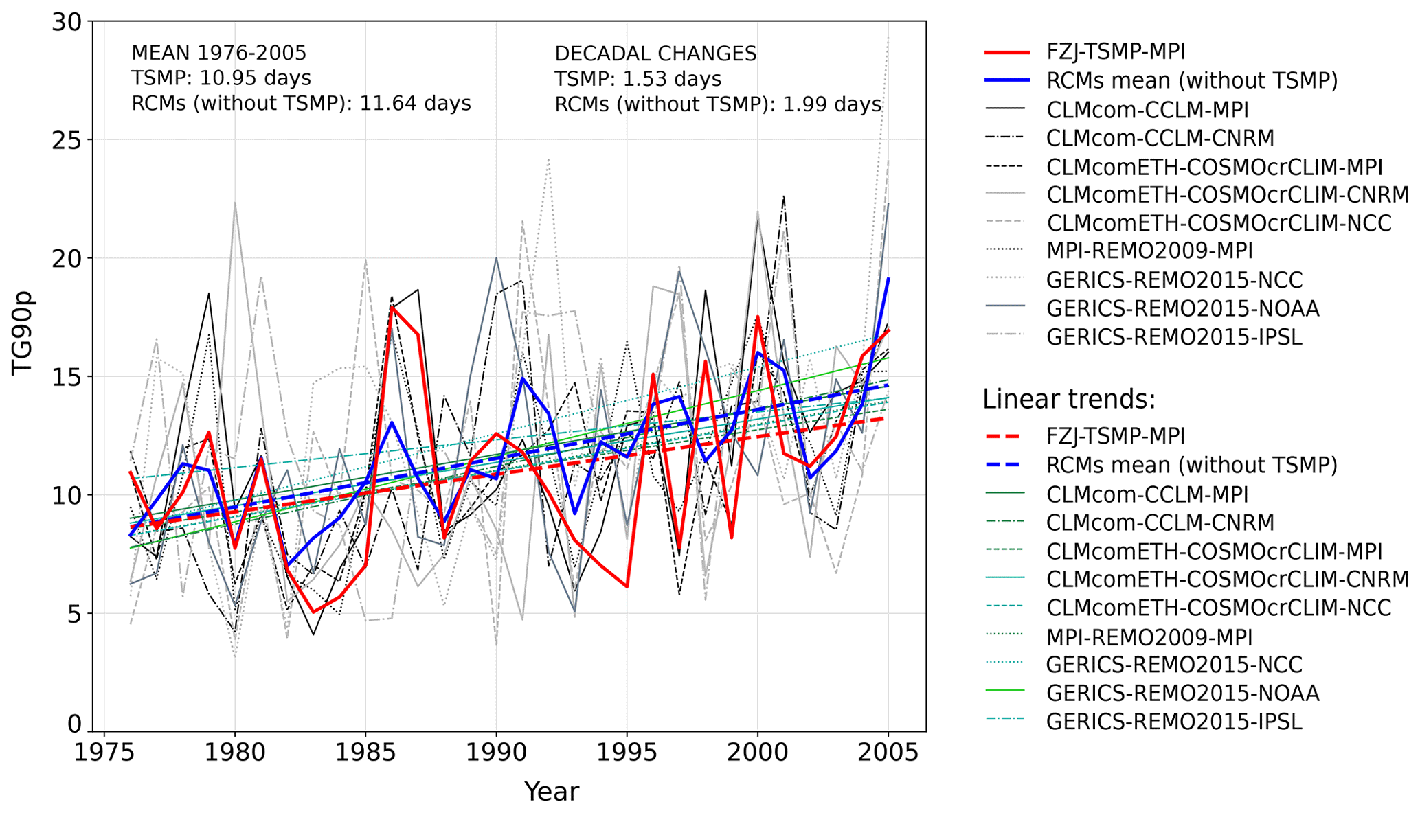
Figure 3Time series and linear trends of the summer TG90p index, averaged over the focus domain, during 1976–2005 in relation to the reference period 1961–1990, in the TSMP simulation and the CORDEX ensemble. The solid and dashed red lines show the summer mean TG90p index and its linear trend from the TSMP simulation. The black and grey lines represent the summer mean TG90p index from the GCM–RCM of the CORDEX ensemble and the green lines are their linear trends, respectively. The summer TG90p index averaged over the CORDEX multi-model ensemble is shown with the solid blue line, and its linear trend is shown with the dashed blue line.
3.2 Heat events of different durations
The summer seasonal number of heat events (i.e., series of consecutive hot days) of different durations occurring on average between 1976 and 2005 in the focus domain in TSMP and the CORDEX ensemble is shown in Fig. 7a. In the considered GCM–RCM multi-model ensemble, the mean number of heat events of any duration per summer in the focus domain ranges from 4.18 to 4.86 heat events, with TSMP simulating 4.66 heat events. The ratios of the number of heat events between the CORDEX RCMs and TSMP (see blue lines in Fig. 7a) are greater than 1 for heat waves, i.e., heat events lasting at least 6 d, and increases towards the heat waves of long durations. This behaviour indicates that TSMP systematically simulates the least number of heat waves compared to the CORDEX ensemble. An intercomparison of the RCMs from the CORDEX ensemble shows that COSMO tends to simulate fewer heat waves on average over the focus domain compared to REMO.
The GCM–RCM multi-model ensemble leads to different spatial distributions of heat waves (Fig. 8). TSMP generates the smoothest spatial distribution of the number of heat waves, resulting in the smallest regional differences compared to the CORDEX ensemble (see indicated standard deviations in Fig. 8). The decadal number of summer heat waves on average over the focus domain ranges from 3.25 to 5.09 in the GCM–RCM multi-model ensemble, with the lowest value in TSMP (Table B3 in Appendix B). When comparing TSMP with the CORDEX RCMs driven by MPI-ESM-LR, the TSMP simulation has most of the heat waves located in central Europe, while the RCMs from the CORDEX ensemble simulate the highest number of heat waves towards southern Europe. The largest differences occur in the Iberian Peninsula, with 2.51 heat waves per decade in TSMP and between 4.88 and 5.25 heat waves per decade in the RCMs driven by MPI-ESM-LR from the CORDEX ensemble.
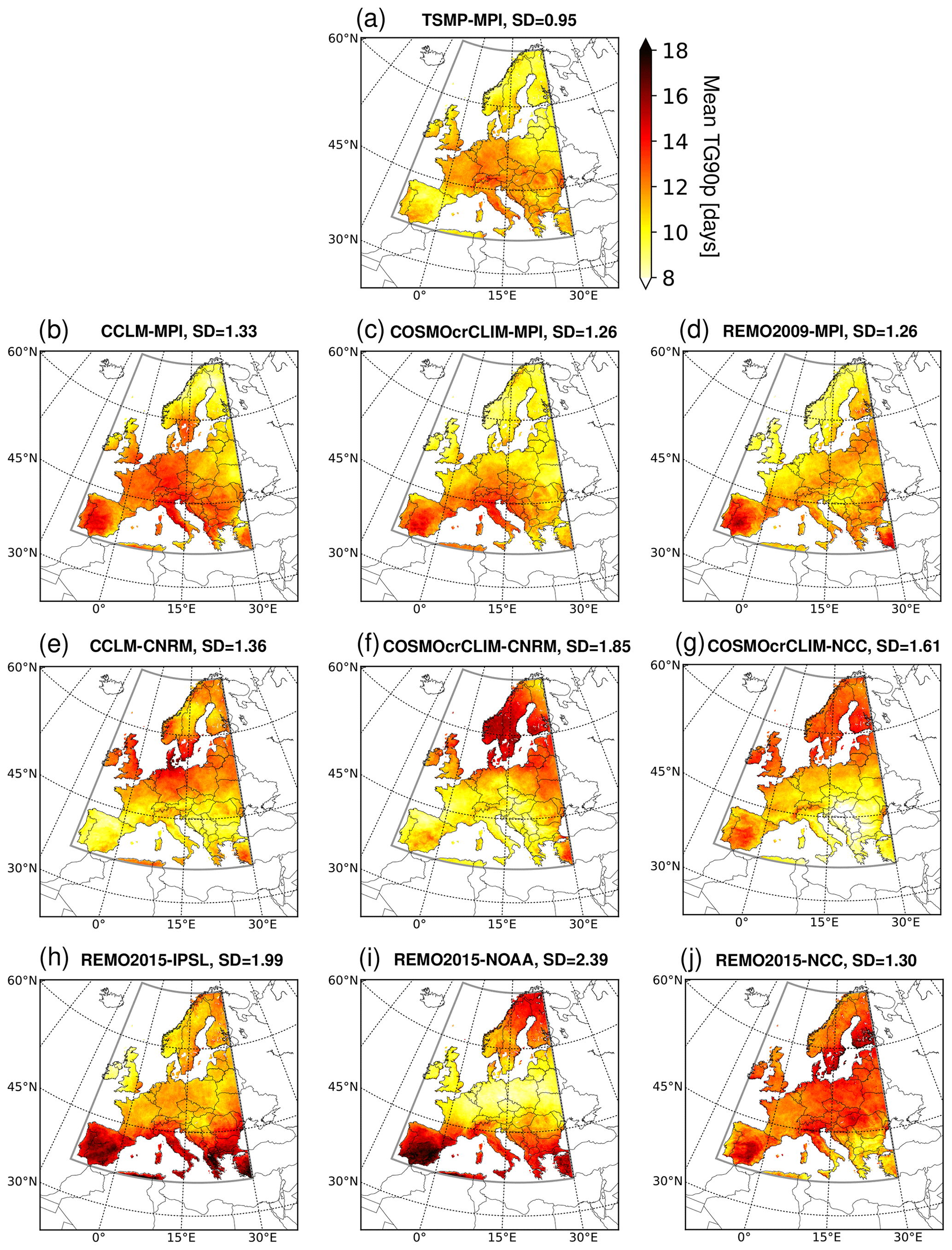
Figure 4Spatial distribution of the summer TG90p index averaged between 1976 and 2005 for TSMP (a) and the CORDEX ensemble (b–j). A standard deviation (SD) of the spatial distribution of the summer TG90p is indicated in every panel.
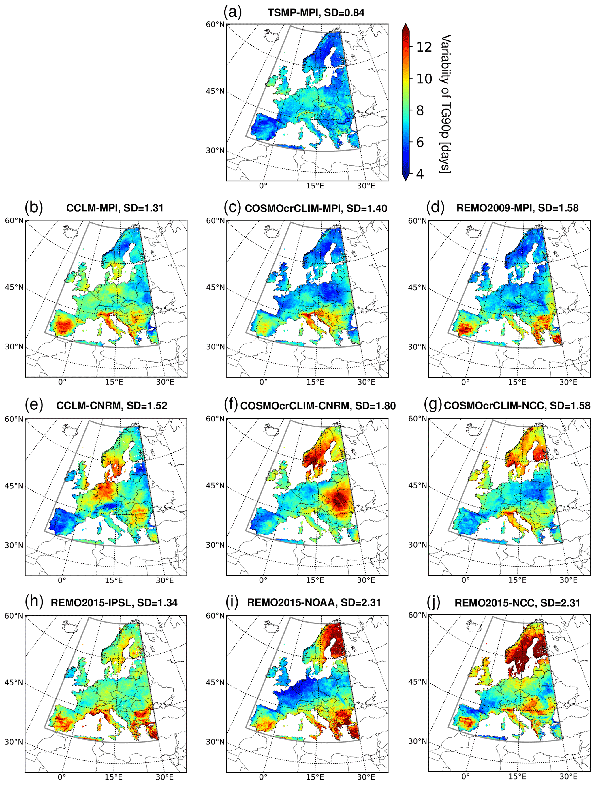
Figure 5Variability of the summer TG90p index, calculated for each grid element from the time series of the summer mean TG90p index between 1976 and 2005 as standard deviation, for TSMP (a) and the CORDEX ensemble (b–j). A standard deviation (SD) of the spatial distribution of the variability of the summer TG90p index is indicated in every panel.
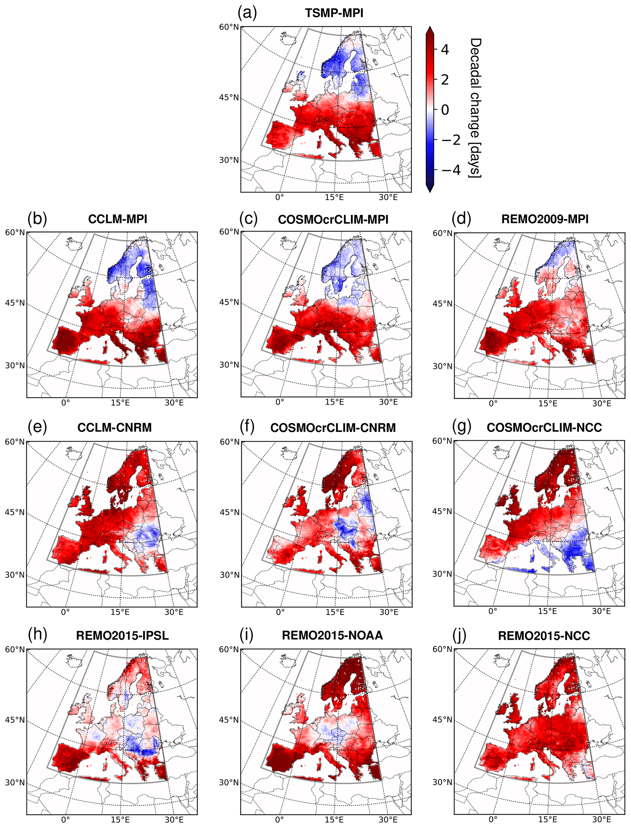
Figure 6Spatial distribution of the decadal change in the summer TG90p index, calculated for each grid element from the time series of the summer mean TG90p index between 1976 and 2005 as a linear trend, for TSMP (a) and the CORDEX ensemble (b–j).
The contribution of heat waves to the total number of hot days is presented in Fig. 9. Here, heat waves account for from 22.38 % to 34.40 % of hot days on average in the focus domain, with TSMP giving the lowest value (Table B2 in Appendix B). The highest fraction of hot days attributed to heat waves prevails in Scandinavia, from 26.50 % to 39.04 %, while eastern Europe tends to be the region with the lowest number of hot days associated with heat waves. From the comparison of TSMP with the RCMs driven by MPI-ESM-LR, the largest differences in the proportion of hot days belonging to heat waves are observed in the Iberian Peninsula, where TSMP simulates 17.47 % and the RCMs driven by MPI-ESM-LR from the CORDEX ensemble simulate between 31.19 % and 33.04 %.
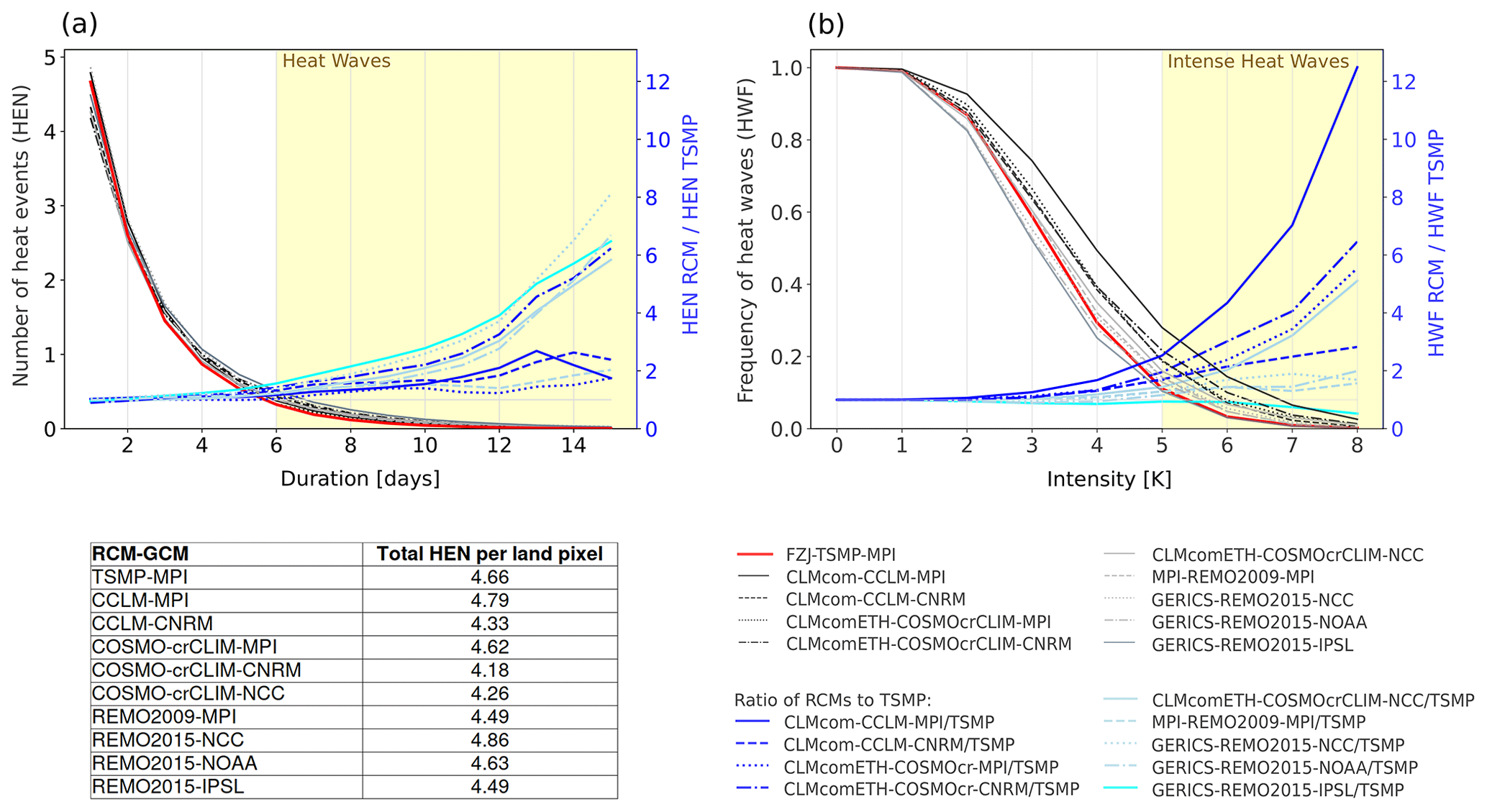
Figure 7(a) Mean number of summer heat events (HEN, y axis) of duration equal to or greater than a given number of days (x axis) as a function of this number of days. The averaging is performed over the focus domain and the total number of investigated years, i.e., 30 years, from 1976–2005. HEN is shown with the solid red line for TSMP and with the black and grey lines for the CORDEX ensemble. The total HEN occurring on average over the summer season in the focus domain in each RCM considered is given in the inset table. (b) Frequency of heat waves (HWF, y axis) with intensities equal to or higher than a value indicated on the abscissa, occurring in the focus domain from 1976–2005, as a function of this intensity. HWF is shown with the red solid line for TSMP and with the black and grey lines for the CORDEX ensemble. Panels (a) and (b) also show the ratios between the RCMs from the CORDEX ensemble and TSMP for HEN and HWN values, and are represented by the blue lines, respectively. Data are taken from the summer seasons between 1976 and 2005 relative to the reference period 1961–1990 in each RCM. The representation of the dependencies is adopted from the work of Vautard et al. (2013).
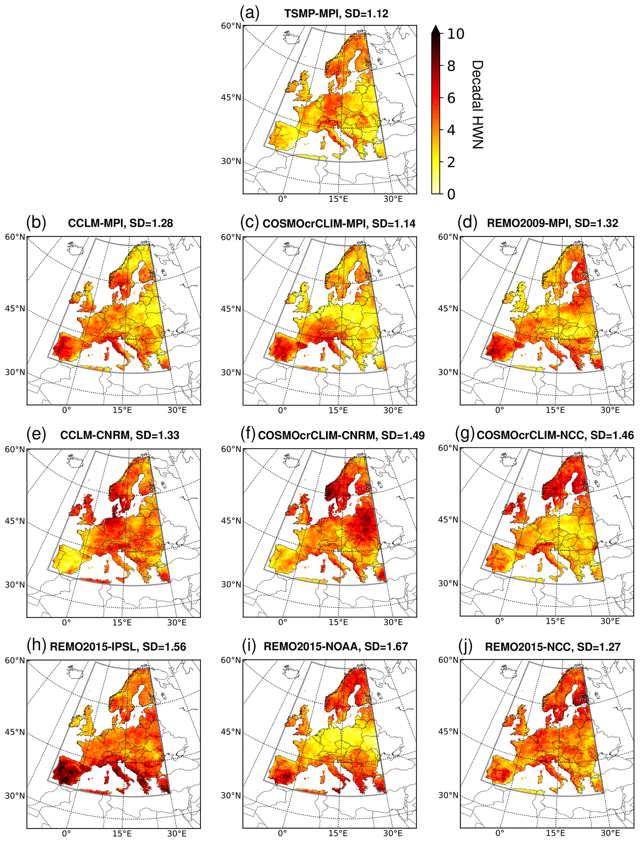
Figure 8Spatial distribution of the decadal number of summer heat waves (HWN), calculated from the data between 1976 and 2005 relative to the reference period 1961–1990, for TSMP (a) and the CORDEX ensemble (b–j). A standard deviation (SD) of the spatial distribution of the decadal HWN is indicated in every panel.
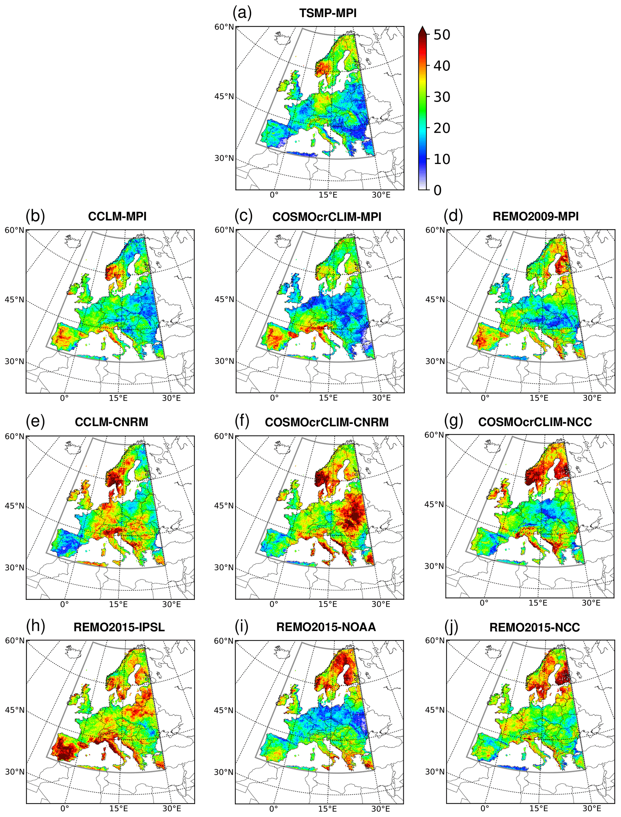
Figure 9Contribution of heat waves to the number of hot days (%), calculated from the total number of heat waves and hot days accumulated between 1976 and 2005, for TSMP (a) and the CORDEX ensemble (b–j).
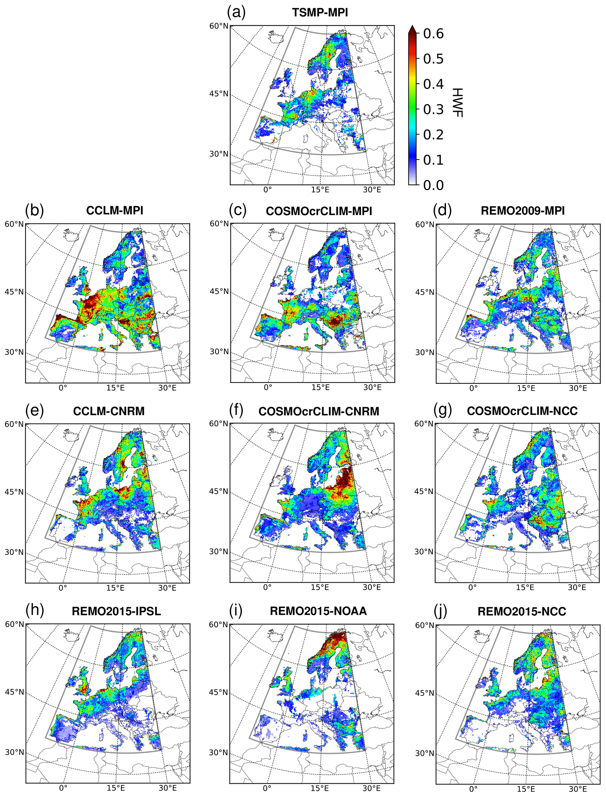
Figure 10Frequency of intense heat waves (HWF), i.e., heat waves with intensities of at least 5 K, relative to the total number of heat waves occurring between 1976 and 2005 in each RCM. The HWF distribution is shown for TSMP (a) and the CORDEX ensemble (b–j).
3.3 Heat waves of different intensities
The dependencies of the frequency of heat waves that occurred in the focus domain in the period from 1976–2005 on their intensities are shown in Fig. 7b. The maximum frequency of heat waves is equal to 1 for an intensity greater than 0 because all heat waves are taken into account for each RCM. The ratios of heat wave frequencies between the CORDEX RCMs and TSMP (see blue lines in Fig. 7b) increase towards intense heat waves, i.e., heat waves with an intensity of at least 5 K, except for REMO2015 driven by IPSL-CM5A-LR. TSMP shows a systematic behaviour to simulate less intense heat waves on average in the focus domain compared to the CORDEX ensemble. Note that the largest discrepancy in the frequency of heat waves with TSMP is found in CCLM4-8-17 driven by MPI-ESM-LR, up to a factor of 12 or even more depending on the intensity considered, although TSMP is the most compatible with CCLM4-8-17 in the considered GCM–RCM multi-model ensemble. An intercomparison of the RCMs within the CORDEX ensemble shows that COSMO tends to simulate more intense heat waves than REMO on average over the focus domain.
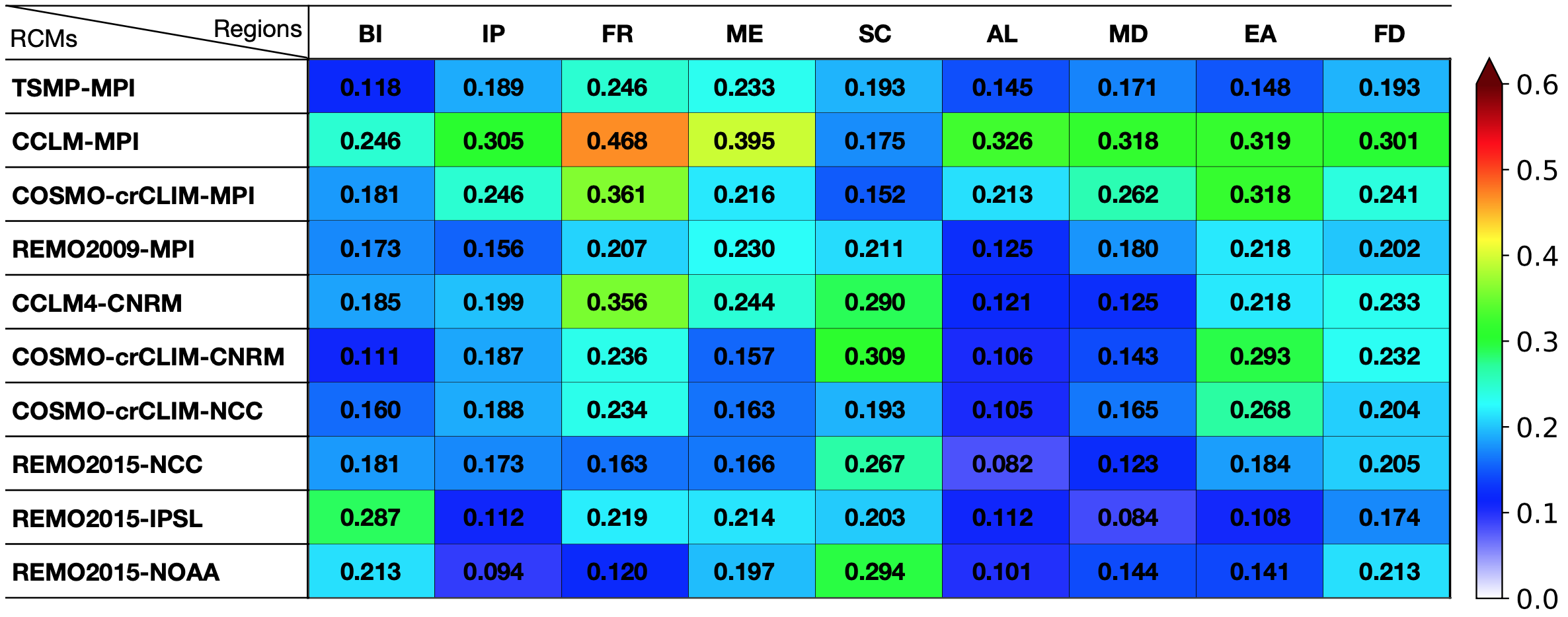
The most intense heat waves are located in western and northern Europe in the majority of RCMs of the considered multi-model ensemble (Fig. 10). The frequency of intense heat waves occurring in the focus domain between 1976 and 2005 ranges from 0.174 to 0.301, i.e., from 17.4 % to 30.1 % heat waves are intense in the GCM–RCM multi-model ensemble, with TSMP giving the second lowest value after REMO2015 driven by IPSL-CM5A-LR (Table B3 in Appendix B). As already noted, TSMP has the largest discrepancy in the frequency of heat waves with CCLM4-8-17 driven by MPI-ESM-LR, with particularly large differences in the France PRUDENCE region, where TSMP leads to a frequency of 0.246 and CCLM4-8-17 to 0.468. It is important to point out that the regions with the highest number of intense heat waves do not necessarily coincide with the regions that experience the most heat waves. The origin of such behaviour should be further investigated and is beyond the scope of this analysis.
4.1 Physical mechanisms
Compared to the simplified 1D free-drainage approach, the physics-based 3D groundwater representation in TSMP results in regionally shallower groundwater levels, causing wetter soils (Keune et al., 2016). This leads to enhanced evapotranspiration by an increase in the latent heat flux and a decrease in the sensible heat flux (e.g., Maxwell and Condon, 2016). In turn, higher evapotranspiration causes moistening of the lower atmosphere and increases downward longwave radiation due to the greenhouse effect of water vapour; on the other hand, it causes cooling of the surface and reduces outgoing surface longwave radiation (e.g., Pal and Eltahir, 2001; Yang et al., 2018). Additionally, higher evapotranspiration may lead to moist convection or rainfall and further affect soil moisture. The simplified representation of groundwater dynamics in RCMs leads to the opposite effect, i.e., deeper groundwater levels and drier soils, overestimating the coupling between the land surface and the atmosphere. This causes a decrease in cloud cover and an enhancement of net solar radiation, thus increasing near-surface temperatures, which further reduces soil moisture (e.g., Vogel et al., 2018; Hartick et al., 2022).
The results of our study suggest that the response of summer heat events to the physics-based 3D representation of groundwater in TSMP varies from year to year (see Fig. 3). Unlike the RCMs from the CORDEX ensemble, the explicit representation of groundwater incorporated into the TSMP model accounts for long-term soil moisture memory effects (Hartick et al., 2021). Soil moisture memory contributes to either increasing the probability of a subsurface water storage deficit in regions that have had a subsurface water deficit in the previous year due to drought conditions, thereby increasing the occurrence of heat events, or, conversely, buffering droughts and reducing the number of heat events (e.g., Martínez-de la Torre and Miguez-Macho, 2019; Hartick et al., 2021; Dirmeyer et al., 2021). Droughts can also remotely affect areas outside the drought region through changes in atmospheric circulation and advection of air masses and further contribute to the evolution of heat events (Fischer et al., 2007).
Considering an extended period of 30 years, from 1976–2005, TSMP driven by MPI-ESM-LR shows systematic differences in the distribution of heat events characteristics (i.e., duration, intensity, frequency) compared to the CORDEX ensemble by simulating fewer, shorter, and less severe heat events in Europe with smaller regional differences. We relate this behaviour to a more realistically simulated soil moisture and thus evapotranspiration in TSMP (see also Furusho-Percot et al., 2022). In addition, the tendency for different responses in the different PRUDENCE regions can be explained by the soil moisture–temperature feedbacks associated with evaporative regimes: energy-limited in northern Europe (i.e., a wet regime in which land evaporation is mainly controlled by incoming radiation) and moisture-limited prevailing in southern Europe (i.e., a dry regime in which land evaporation increases or decreases in response to increased or decreased soil moisture content) (e.g., Seneviratne et al., 2010; Haghighi et al., 2018; Jach et al., 2022). The comparison of TSMP with the most compatible RCM from the CORDEX ensemble, i.e., CCLM4-8-17 forced by MPI-ESM-LR, shows that groundwater representation has a particularly strong influence on the intensity of heat waves versus their duration (see Fig. 7); the physical mechanisms of this phenomenon require further investigation and are beyond the scope of this study.
4.2 Methodology limitations
In order to capture the full range of divergence in simulation results over the historical period, and hence potential uncertainties in the climate projections, it is necessary to combine as many different GCM–RCM pairs as possible (e.g., Déqué et al., 2012; Christensen and Kjellström, 2020). Often, certain RCMs and GCMs are overrepresented compared to others, even leading to contradictions in climate change signals (Turco et al., 2013; Fernández et al., 2019). Note that the role of the GCM-imposed boundary conditions is generally greater that the role of RCMs (Déqué et al., 2007; Evin et al., 2021). In this study, a limited number of GCM–RCM pairs (see Table 1) were used for comparison with TSMP; therefore, expanding the multi-model GCM–RCM ensemble or using other GCM–RCM pairs may lead to quantitatively different results.
It is important to emphasize that the GCM–RCM multi-model ensemble is not intended for direct comparison between individual ensemble members, as it includes different RCMs in combination with different driving GCMs. Due to the interplay of various factors (e.g., conceptual and structural differences between models, model set-up, different physical parameterizations, internal variability, boundary conditions, representation of the subsurface–land–atmosphere feedbacks) in addition to groundwater representation, it is challenging to reveal the exact cause–effect relationships between the explicit groundwater representation and simulated heat events. However, considering an extended period of 30 years allows us to draw statistical conclusions.
To quantify the exact impact of the explicit representation of groundwater in TSMP and minimize the impact of other factors, it would be necessary to additionally conduct a long-term TSMP climate simulation with a simplified 1D free-drainage approach for groundwater representation and then compare the affected processes within TSMP rather than across the multi-model GCM–RCM ensemble. Since our study uses the same version of the TSMP model as in Keune et al. (2016), which have already shown the effect of 3D groundwater dynamics on the water and energy balance, and taking into account the high computational cost, the additional TSMP simulation with simplified groundwater representation is not feasible. The multi-model GCM–RCM ensemble analysis performed in this study provides valuable insights into the consistency between the new dataset of TSMP driven by MPI-ESM-LR and the CORDEX ensemble.
Note that the results of this research are limited to the definitions used (e.g., hot day, heat event, heat wave, intense heat wave), the method of percentile estimation, and the choice of the investigated and reference time periods. For instance, Sulikowska and Wypych (2020) indicate that different variations in the metrics lead to different distributions of hot days during the summer season in Europe.
We presented a first-of-its-kind dataset of TSMP simulation driven by the CMIP5 MPI-ESM-LR GCM boundary conditions, in the context of dynamical downscaling of GCMs by RCMs for climate change studies. Unlike most RCMs, TSMP is a fully coupled regional climate system model with an explicit representation of groundwater, enabling complete water and energy cycles to be considered. We examined the role of groundwater representation for heat events in a multi-model ensemble of 10 different GCM–RCM pairs by comparing TSMP results and those from the CORDEX experiment with simplified groundwater representation. Specifically, we performed a statistical analysis of the characteristics of heat events (i.e., duration, intensity, frequency) over Europe during the summer seasons between 1976 and 2005 in relation to the reference period of 1961–1990.
The characteristics of heat events simulated by TSMP are consistent with the CORDEX ensemble, although systematic differences are observed, which we attribute to an explicit representation of groundwater in TSMP. Our findings suggest that the integrated 3D physics-based representation of groundwater in TSMP leads to a reduction in the number of hot summer days, their interannual variability, and decadal change and causes smaller regional differences compared to the CORDEX ensemble. The explicit representation of groundwater also influences simulated heat waves, resulting in a decrease in the number of heat waves and a reduction in their duration and intensity compared to the CORDEX ensemble. From the comparison of TSMP and the CORDEX RCMs driven by MPI-ESM-LR, the Iberian Peninsula is the most sensitive region with respect to groundwater representation.
This study clearly indicates that a coupled regional climate system model with 3D groundwater dynamics systematically simulates a different climatology of heat events in Europe compared to RCMs with simplified representation of groundwater. The results emphasize the importance of hydrological processes for reliable climate modelling and for reducing biases in the duration, intensity, and frequency of simulated heat waves in particular, and they are of further importance when assessing uncertainties in climate change projections.
Table A1Summer TG90p index (d) averaged between 1976 and 2005 in the GCM–RCM multi-model ensemble for the focus domain (FD; see Fig. 2) and the PRUDENCE regions: British Isles (BI), Iberian Peninsula (IP), France (FR), mid-Europe (ME), Scandinavia (SC), Alps (AL), Mediterranean (MD), and eastern Europe (EA). Refer to Fig. 4 for the spatial distribution.
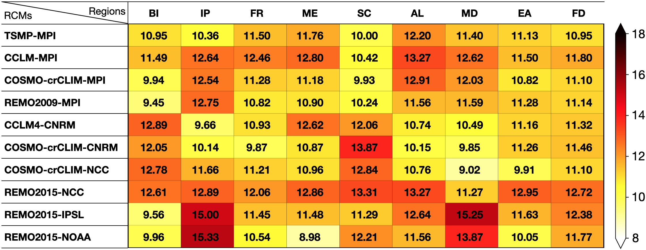
Table A2Variability of the summer TG90p index (d), calculated from the data between 1976 and 2005 in the GCM–RCM multi-model ensemble, for the focus domain (FD; see Fig. 2) and the PRUDENCE regions: British Isles (BI), Iberian Peninsula (IP), France (FR), mid-Europe (ME), Scandinavia (SC), Alps (AL), Mediterranean (MD), and eastern Europe (EA). Refer to Fig. 5 for the spatial distribution.
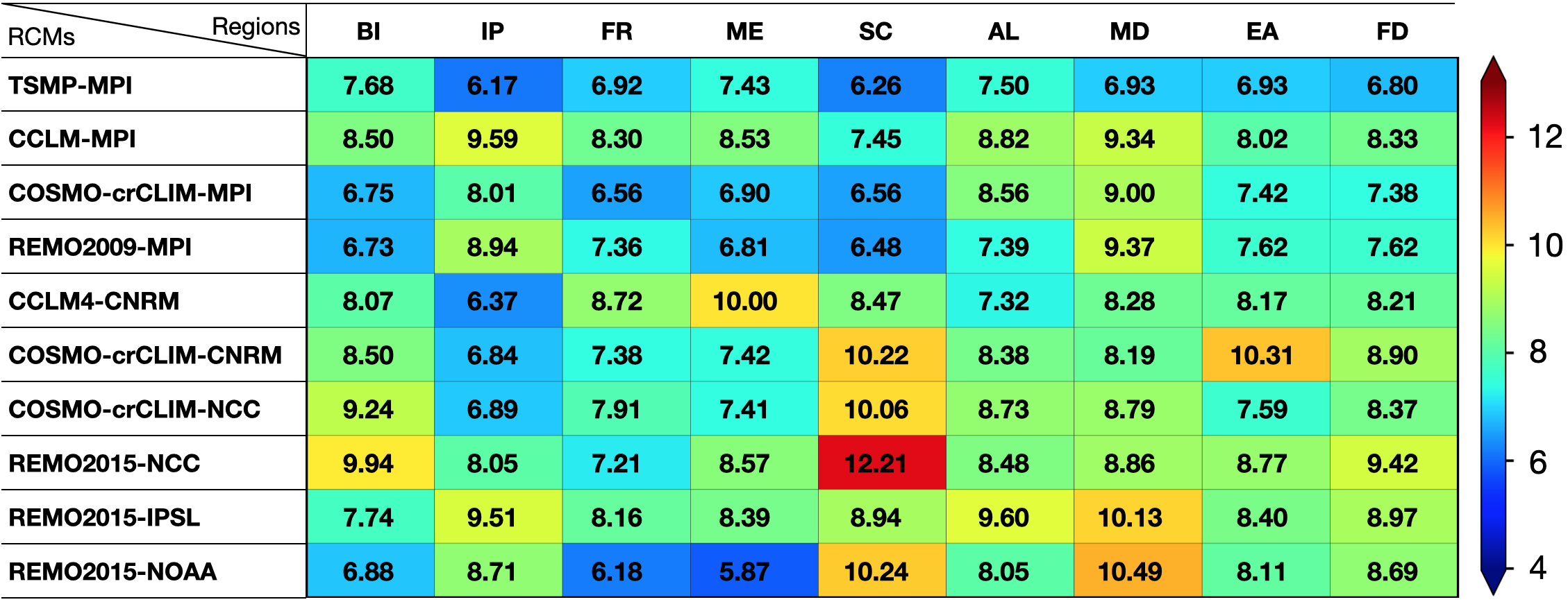
Table A3Decadal change in the summer TG90p index (d), calculated from the data between 1976 and 2005 in the GCM–RCM multi-model ensemble, for the focus domain (FD; see Fig. 2) and the PRUDENCE regions: British Isles (BI), Iberian Peninsula (IP), France (FR), mid-Europe (ME), Scandinavia (SC), Alps (AL), Mediterranean (MD), and eastern Europe (EA). Refer to Fig. 6 for the spatial distribution.
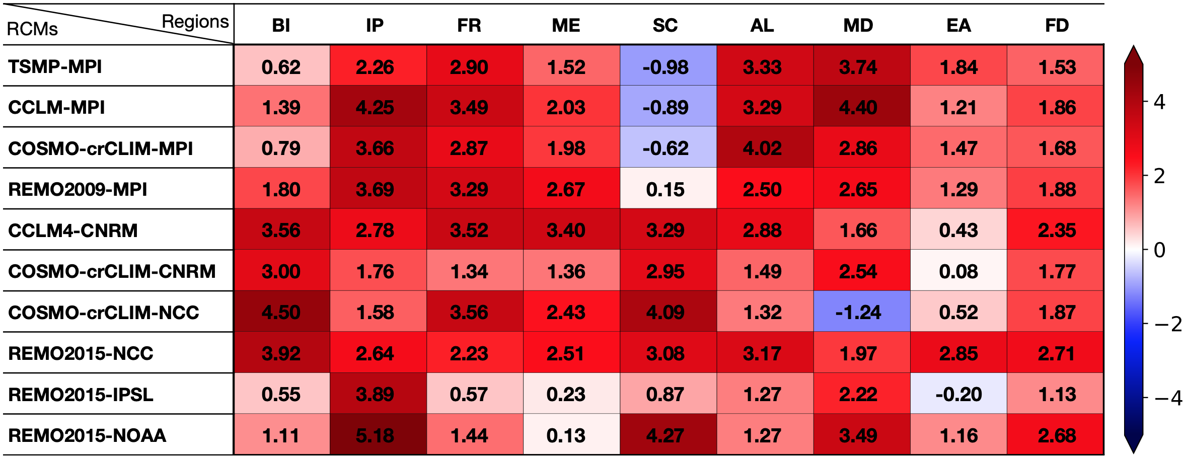
Table B1Decadal number of summer heat waves, calculated from the data between 1976 and 2005 in the GCM–RCM multi-model ensemble, for the focus domain (FD; see Fig. 2) and the PRUDENCE regions: British Isles (BI), Iberian Peninsula (IP), France (FR), mid-Europe (ME), Scandinavia (SC), Alps (AL), Mediterranean (MD), and eastern Europe (EA). Refer to Fig. 8 for the spatial distribution.
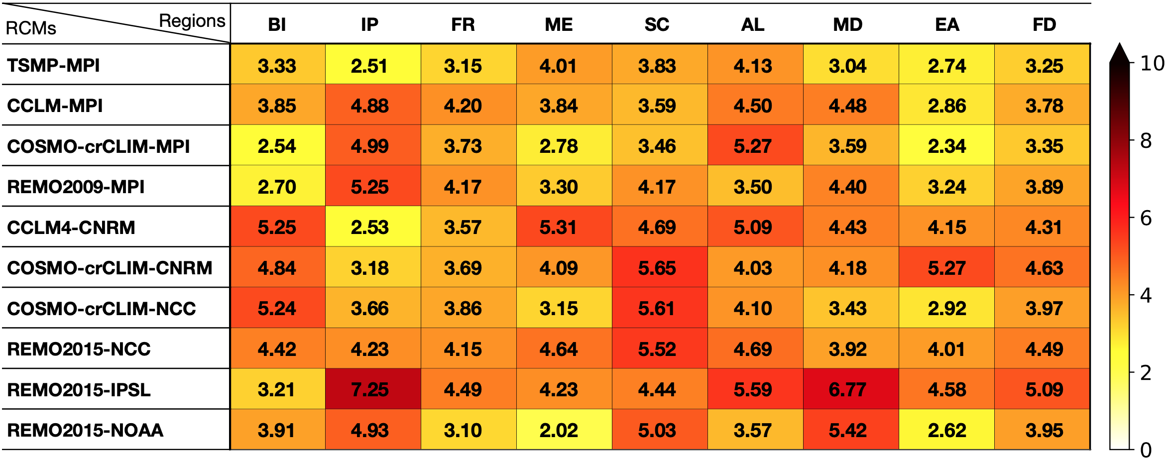
Table B2Contribution of heat waves to the number of hot days (%), based on the data from 1976–2005 in the GCM–RCM multi-model ensemble, for the focus domain (FD; see Fig. 2) and the PRUDENCE regions: British Isles (BI), Iberian Peninsula (IP), France (FR), mid-Europe (ME), Scandinavia (SC), Alps (AL), Mediterranean (MD), and eastern Europe (EA). Refer to Fig. 9 for the spatial distribution.
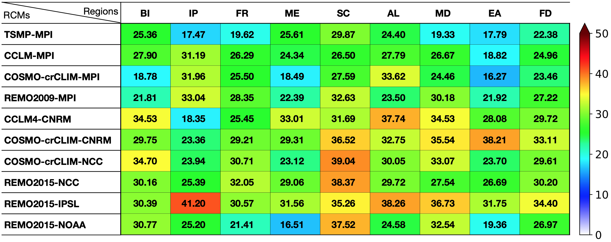
Table B3Frequency of intense heat waves, calculated from the data between 1976 and 2005 in the GCM–RCM multi-model ensemble, for the focus domain (FD; see Fig. 2) and the PRUDENCE regions: British Isles (BI), Iberian Peninsula (IP), France (FR), mid-Europe (ME), Scandinavia (SC), Alps (AL), Mediterranean (MD), and eastern Europe (EA). Refer to Fig. 10 for the spatial distribution.
The TSMP v1.2.2 used in this work is available via the following Git repository: https://github.com/HPSCTerrSys/TSMP (last access: 15 December 2022). The dataset of TSMP driven by MPI-ESM-LR r1i1p1 can be accessed as open-access research data at https://doi.org/10.26165/JUELICH-DATA/9S3V5K (Poshyvailo-Strube et al., 2023).
The study was designed by SK with contributions by KG, LPS, and NW. LPS performed the model simulations and data processing, NW provided technical and programming support, and CH provided configuration and workflow support. The analysis was developed and conducted by LPS with further inputs from SK and KG. LPS wrote the manuscript. All co-authors contributed to the interpretation of the results, active discussions, and revisions of the paper. The work was done under the supervision of SK.
The contact author has declared that none of the authors has any competing interests.
Publisher’s note: Copernicus Publications remains neutral with regard to jurisdictional claims made in the text, published maps, institutional affiliations, or any other geographical representation in this paper. While Copernicus Publications makes every effort to include appropriate place names, the final responsibility lies with the authors.
This research was funded by the Helmholtz Association of German Research Centres (HGF) under the HI-CAM project (Helmholtz Initiative Climate Adaptation and Mitigation) and by the German Ministry of Education and Research (Bundesministerium für Bildung und Forschung, BMBF) under the ClimXtreme project (grant no. 01LP1903G). We are grateful to the Max Planck Institute for performing MPI-ESM-LR r1i1p1 GCM experiment and the German Climate Computing Centre (DKRZ) for providing the MPI-ESM-LR dataset. We thank the EURO-CORDEX climate modelling groups for producing their model outputs and making them available. The authors gratefully acknowledge the Earth System Modelling Project (ESM) for funding this work by providing computing time on the ESM partition of the supercomputer JUWELS at the Jülich Supercomputing Centre (JSC) under the ESM project ID JIBG35. In addition, we thank the Centre for High-Performance Scientific Computing in Terrestrial Systems (Geoverbund ABC/J, http://www.hpsc-terrsys.de, last access: 1 December 2023) and the JSC for the computational support. Finally, we thank the two anonymous reviewers for their constructive comments that helped improve this article.
The article processing charges for this open-access publication were covered by the Forschungszentrum Jülich GmbH.
This paper was edited by Anping Chen and reviewed by two anonymous referees.
Alexander, L. V., Zhang, X., Peterson, T. C., Caesar, J., Gleason, B., Klein Tank, A. M. G., Haylock, M., Collins, D., Trewin, B., Rahimzadeh, F., Tagipour, A., Rupa Kumar, K., Revadekar, J., Griffiths, G., Vincent, L., Stephenson, D. B., Burn, J., Aguilar, E., Brunet, M., Taylor, M., New, M., Zhai, P., Rusticucci, M., and Vazquez-Aguirre, J. L.: Global observed changes in daily climate extremes of temperature and precipitation, J. Geophys. Res.-Atmos., 111, D05109, https://doi.org/10.1029/2005JD006290, 2006. a
Amengual, A., Homar, V., Romero, R., Brooks, H., Ramis, C., Gordaliza, M., and Alonso, S.: Projections of heat waves with high impact on human health in Europe, Glob. Planet. Change, 119, 71–84, https://doi.org/10.1016/j.gloplacha.2014.05.006, 2014. a
Baldauf, M., Seifert, A., Förstner, J., Majewski, D., Raschendorfer, M., and Reinhardt, T.: Operational Convective-Scale Numerical Weather Prediction with the COSMO Model: Description and Sensitivities, Mon. Weather Rev., 139, 3887–3905, https://doi.org/10.1175/MWR-D-10-05013.1, 2011. a
Barlage, M., Tewari, M., Chen, F., Miguez-Macho, G., Yang, Z.-L., and Niu, G.-Y.: The effect of groundwater interaction in North American regional climate simulations with WRF/Noah-MP, Climatic Change, 129, 485–498, https://doi.org/10.1007/s10584-014-1308-8, 2015. a
Barlage, M., Chen, F., Rasmussen, R., Zhang, Z., and Miguez-Macho, G.: The Importance of Scale-Dependent Groundwater Processes in Land-Atmosphere Interactions Over the Central United States, Geophys. Res. Lett., 48, e2020GL092171, https://doi.org/10.1029/2020GL092171, 2021. a, b
Barriopedro, D., Fischer, E. M., Luterbacher, J., Trigo, R. M., and García-Herrera, R.: The Hot Summer of 2010: Redrawing the Temperature Record Map of Europe, Science, 332, 220–224, https://doi.org/10.1126/science.1201224, 2011. a
Barriopedro, D., García-Herrera, R., Ordóñez, C., Miralles, D. G., and Salcedo-Sanz, S.: Heat Waves: Physical Understanding and Scientific Challenges, Rev. Geophys., 61, e2022RG000780, https://doi.org/10.1029/2022RG000780, 2023. a
Bellprat, O., Kotlarski, S., Lüthi, D., Elía, R. D., Frigon, A., Laprise, R., and Schär, C.: Objective Calibration of Regional Climate Models: Application over Europe and North America, J. Clim., 29, 819–838, https://doi.org/10.1175/JCLI-D-15-0302.1, 2016. a
Bentsen, M., Bethke, I., Debernard, J. B., Iversen, T., Kirkevåg, A., Seland, Ø., Drange, H., Roelandt, C., Seierstad, I. A., Hoose, C., and Kristjánsson, J. E.: The Norwegian Earth System Model, NorESM1-M – Part 1: Description and basic evaluation of the physical climate, Geosci. Model Dev., 6, 687–720, https://doi.org/10.5194/gmd-6-687-2013, 2013. a
Christensen, J. H. and Christensen, O. B.: A summary of the PRUDENCE model projections of changes in European climate by the end of this century, Climatic Change, 81, 7–30, https://doi.org/10.1007/s10584-006-9210-7, 2007. a
Christensen, O. B. and Kjellström, E.: Partitioning uncertainty components of mean climate and climate change in a large ensemble of European regional climate model projections, Clim. Dynam., 54, 4293–4308, https://doi.org/10.1007/s00382-020-05229-y, 2020. a
Christidis, N., Jones, G., and Stott, P.: Dramatically increasing chance of extremely hot summers since the 2003 European heatwave, Nat. Climatic Change, 5, 46–50, https://doi.org/10.1038/nclimate2468, 2015. a
Cornes, R. C., van der Schrier, G., van den Besselaar, E. J. M., and Jones, P. D.: An Ensemble Version of the E-OBS Temperature and Precipitation Data Sets, J. Geophys. Res.-Atmos., 123, 9391–9409, https://doi.org/10.1029/2017JD028200, 2018. a
Daac, L.: Global 30 arc-second elevation data set GTOPO30, Land process distributed active archive center, https://www.usgs.gov/centers/eros/science/ (last access: 15 December 2022), 2004. a
Dee, D. P., Uppala, S. M., Simmons, A. J., Berrisford, P., Poli, P., Kobayashi, S., Andrae, U., Balmaseda, M. A., Balsamo, G., Bauer, P., Bechtold, P., Beljaars, A. C. M., van de Berg, L., Bidlot, J., Bormann, N., Delsol, C., Dragani, R., Fuentes, M., Geer, A. J., Haimberger, L., Healy, S. B., Hersbach, H., Hólm, E. V., Isaksen, L., Kallberg, P., Koehler, M., Matricardi, M., McNally, A. P., Monge-Sanz, B. M., Morcrette, J.-J., Park, B.-K., Peubey, C., de Rosnay, P., Tavolato, C., Thépaut, J.-N., and Vitart, F.: The ERA-Interim reanalysis: configuration and performance of the data assimilation system, Q. J. Roy. Meteor. Soc., 137, 553–597, https://doi.org/10.1002/qj.828, 2011. a
Déqué, M., Rowell, D. P., Lüthi, D., Giorgi, F., Christensen, J. H., Rockel, B., Jacob, D., Kjellström, E., de Castro, M., and van den Hurk, B.: An intercomparison of regional climate simulations for Europe: assessing uncertainties in model projections, Climatic Change, 81, 53–70, https://doi.org/10.1007/s10584-006-9228-x, 2007. a
Déqué, M., Somot, S., Sanchez-Gomez, E., Goodess, C. M., Jacob, D., Lenderink, G., and Christensen, O. B.: The spread amongst ENSEMBLES regional scenarios: regional climate models, driving general circulation models and interannual variability, Climatic Change, 38, 951–964, https://doi.org/10.1007/s00382-011-1053-x, 2012. a
Dirmeyer, P. A., Balsamo, G., Blyth, E. M., Morrison, R., and Cooper, H. M.: Land-Atmosphere Interactions Exacerbated the Drought and Heatwave Over Northern Europe During Summer 2018, AGU Advances, 2, e2020AV000283, https://doi.org/10.1029/2020AV000283, 2021. a, b, c
Dufresne, J. -L., Foujols, M. -A., Denvil, S., Caubel, A., Marti, O., Aumont, O., Balkanski, Y., Bekki, S., Bellenger, H., Benshila, R., Bony, S., Bopp, L., Braconnot, P., Brockmann, P., Cadule, P., Cheruy, F., Codron, F., Cozic, A., Cugnet, D., de Noblet, N., Duvel, J. -P., Ethé, C., Fairhead, L., Fichefet, T., Flavoni, S., Friedlingstein, P., Grandpeix, J. -Y., Guez, L., Guilyardi, E., Hauglustaine, D., Hourdin, F., Idelkadi, A., Ghattas, J., Joussaume, S., Kageyama, M., Krinner, G., Labetoulle, S., Lahellec, A., Lefebvre, M. -P., Lefevre, F., Levy, C., Li, Z. X., Lloyd, J., Lott, F., Madec, G., Mancip, M., Marchand, M., Masson, S., Meurdesoif, Y., Mignot, J., Musat, I., Parouty, S., Polcher, J., Rio, C., Schulz, M., Swingedouw, D., Szopa, S., Talandier, C., Terray, P., Viovy, N., and Vuichard, N.: Climate change projections using the IPSL-CM5 Earth System Model: from CMIP3 to CMIP5, Clim. Dynam., 40, 2123–2165, https://doi.org/10.1007/s00382-012-1636-1, 2013. a
Dunne, J. P., John, J. G., Adcroft, A. J., Griffies, S. M., Hallberg, R. W., Shevliakova, E., Stouffer, R. J., Cooke, W., Dunne, K. A., Harrison, M. J., Krasting, J. P., Malyshev, S. L., Milly, P. C. D., Phillipps, P. J., Sentman, L. T., Samuels, B. L., Spelman, M. J., Winton, M., Wittenberg, A. T., and Zadeh, N.: GFDL’s ESM2 Global Coupled Climate–Carbon Earth System Models. Part I: Physical Formulation and Baseline Simulation Characteristics, J. Clim., 25, 6646–6665, https://doi.org/10.1175/JCLI-D-11-00560.1, 2012. a
Duscher, K., Günther, A., Richts, A., Clos, P., Philipp, U., and Struckmeier, W.: The GIS layers of the “International Hydrogeological Map of Europe 1:1 500 000” in a vector format, Hydrogeol. J., 23, 1867–1875, https://doi.org/10.1007/s10040-015-1296-4, 2015. a
Erdenebat, E. and Tomonori, S.: Role of soil moisture-atmosphere feedback during high temperature events in 2002 over Northeast Eurasia, Prog. Earth. Planet. Sci., 5, 37, https://doi.org/10.1186/s40645-018-0195-4, 2018. a
Evin, G., Somot, S., and Hingray, B.: Balanced estimate and uncertainty assessment of European climate change using the large EURO-CORDEX regional climate model ensemble, Earth Syst. Dynam., 12, 1543–1569, https://doi.org/10.5194/esd-12-1543-2021, 2021. a, b
FAO: FAO/UNESCO Soil Map of the World, Revised Legend, with corrections and updates, World Soil Resources Report 60, FAO, Rome, https://www.fao.org/3/bl892e/bl892e.pdf (last access: 1 December 2022), 1988. a
Fernández, J., Frías, M. D., Cabos, W. D., Cofiño, A. S., Domínguez, M., Fita, L., Gaertner, M. A., García-Díez, M., Gutiérrez, J. M., Jiménez-Guerrero, P., Liguori, G., Montávez, J. P., Romera, R., and Sánchez, E.: Consistency of climate change projections from multiple global and regional model intercomparison projects, Clim. Dynam., 52, 1139–1156, https://doi.org/10.1007/s00382-018-4181-8, 2019. a
Fischer, E. M. and Schär, C.: Consistent geographical patterns of changes in high-impact European heatwaves, Nat. Geosci., 3, 398–403, https://doi.org/10.1038/ngeo866, 2010. a
Fischer, E. M., Seneviratne, S. I., Lüthi, D., and Schär, C.: Contribution of land-atmosphere coupling to recent European summer heat waves, Geophys. Res. Lett., 34, L06707, https://doi.org/10.1029/2006GL029068, 2007. a, b, c
Frich, P., Alexander, L. V., Della-Marta, P., Gleason, B., Haylock, M., Klein Tank, A. M. G., and Peterson, T.: Observed coherent changes in climatic extremes during the second half of the twentieth century, Clim. Res., 19, 193–212, https://doi.org/10.3354/cr019193, 2002. a, b
Friedl, M., McIver, D., Hodges, J., Zhang, X., Muchoney, D., Strahler, A., Woodcock, C., Gopal, S., Schneider, A., Cooper, A., Baccini, A., Gao, F., and Schaaf, C.: Global land cover mapping from MODIS: algorithms and early results, Remote Sens. Environ., 83, 287–302, https://doi.org/10.1016/S0034-4257(02)00078-0, 2002. a
Furusho-Percot, C., Goergen, K., Hartick, C., Kulkarni, K., Keune, J., and Kollet, S.: Pan-European groundwater to atmosphere terrestrial systems climatology from a physically consistent simulation, Sci. Data, 6, 320, https://doi.org/10.1038/s41597-019-0328-7, 2019. a, b, c, d
Furusho-Percot, C., Goergen, K., Hartick, C., Poshyvailo-Strube, L., and Kollet, S.: Groundwater Model Impacts Multiannual Simulations of Heat Waves, Geophys. Res. Lett., 49, e2021GL096781, https://doi.org/10.1029/2021GL096781, 2022. a, b, c, d, e
Gasper, F., Goergen, K., Shrestha, P., Sulis, M., Rihani, J., Geimer, M., and Kollet, S.: Implementation and scaling of the fully coupled Terrestrial Systems Modeling Platform (TerrSysMP v1.0) in a massively parallel supercomputing environment – a case study on JUQUEEN (IBM Blue Gene/Q), Geosci. Model Dev., 7, 2531–2543, https://doi.org/10.5194/gmd-7-2531-2014, 2014. a, b
Giorgetta, M. A., Jungclaus, J., Reick, C. H., Legutke, S., Bader, J., Böttinger, M., Brovkin, V., Crueger, T., Esch, M., Fieg, K., Glushak, K., Gayler, V., Haak, H., Hollweg, H.-D., Ilyina, T., Kinne, S., Kornblueh, L., Matei, D., Mauritsen, T., Mikolajewicz, U., Mueller, W., Notz, D., Pithan, F., Raddatz, T., Rast, S., Redler, R., Roeckner, E., Schmidt, H., Schnur, R., Segschneider, J., Six, K. D., Stockhause, M., Timmreck, C., Wegner, J., Widmann, H., Wieners, K.-H., Claussen, M., Marotzke, J., and Stevens, B.: Climate and carbon cycle changes from 1850 to 2100 in MPI-ESM simulations for the Coupled Model Intercomparison Project phase 5, J. Adv. Model. Earth Syst., 5, 572–597, https://doi.org/10.1002/jame.20038, 2013. a, b, c
Giorgi, F. and Gutowski, W. J.: Regional Dynamical Downscaling and the CORDEX Initiative, Annu. Rev. Env. Resour., 40, 467–490, https://doi.org/10.1146/annurev-environ-102014-021217, 2015. a
Gleeson, T., Moosdorf, N., Hartmann, J., and van Beek, L. P. H.: A glimpse beneath earth's surface: GLobal HYdrogeology MaPS (GLHYMPS) of permeability and porosity, Geophys. Res. Lett., 41, 3891–3898, https://doi.org/10.1002/2014GL059856, 2014. a
Grasselt, R., Schüttemeyer, D., Warrach-Sagi, K., Ament, F., and Simmer, C.: Validation of TERRA-ML with discharge measurements, Meteorol. Z., 17, 763–773, https://doi.org/10.1127/0941-2948/2008/0334, 2008. a
Gutowski, W. J., Giorgi, F., Timbal, B., Frigon, A., Jacob, D., Kang, H.-S., Raghavan, K., Lee, B., Lennard, C., Nikulin, G., O'Rourke, E., Rixen, M., Solman, S., Stephenson, T., and Tangang, F.: WCRP COordinated Regional Downscaling EXperiment (CORDEX): a diagnostic MIP for CMIP6, Geosci. Model Dev., 9, 4087–4095, https://doi.org/10.5194/gmd-9-4087-2016, 2016. a, b
Haghighi, E., Short Gianotti, D. J., Akbar, R., Salvucci, G. D., and Entekhabi, D.: Soil and Atmospheric Controls on the Land Surface Energy Balance: A Generalized Framework for Distinguishing Moisture-Limited and Energy-Limited Evaporation Regimes, Water Resour. Res., 54, 1831–1851, https://doi.org/10.1002/2017WR021729, 2018. a
Hari, V., Rakovec, O., Markonis, Y., Hanel, M., and Kumar, R.: Increased future occurrences of the exceptional 2018–2019 Central European drought under global warming, Sci. Rep., 10, 12207, https://doi.org/10.1038/s41598-020-68872-9, 2020. a
Hartick, C., Furusho-Percot, C., Goergen, K., and Kollet, S.: An Interannual Probabilistic Assessment of Subsurface Water Storage Over Europe Using a Fully Coupled Terrestrial Model, Water Resour. Res., 57, e2020WR027828, https://doi.org/10.1029/2020WR027828, 2021. a, b, c, d
Hartick, C., Furusho-Percot, C., Clark, M. P., and Kollet, S.: An Interannual Drought Feedback Loop Affects the Surface Energy Balance and Cloud Properties, Geophys. Res. Lett., 49, e2022GL100924, https://doi.org/10.1029/2022GL100924, 2022. a
Hawkins, E. and Sutton, R.: The Potential to Narrow Uncertainty in Regional Climate Predictions, Bull. Am. Meteorol. Soc., 90, 1095–1108, https://doi.org/10.1175/2009BAMS2607.1, 2009. a
Horton, R. M., Mankin, J. S., Lesk, C., Coffel, E., and Raymond, C.: Review of Recent Advances in Research on Extreme Heat Events, Curr. Clim. Chang. Rep., 2, 242–259, https://doi.org/10.1007/s40641-016-0042-x, 2016. a, b
Iles, C. E., Vautard, R., Strachan, J., Joussaume, S., Eggen, B. R., and Hewitt, C. D.: The benefits of increasing resolution in global and regional climate simulations for European climate extremes, Geosci. Model Dev., 13, 5583–5607, https://doi.org/10.5194/gmd-13-5583-2020, 2020. a
Jach, L., Schwitalla, T., Branch, O., Warrach-Sagi, K., and Wulfmeyer, V.: Sensitivity of land–atmosphere coupling strength to changing atmospheric temperature and moisture over Europe, Earth Syst. Dynam., 13, 109–132, https://doi.org/10.5194/esd-13-109-2022, 2022. a
Jacob, D. and Podzun, R.: Sensitivity studies with the regional climate model REMO, Meteor. Atmos. Phys., 63, 119–129, https://doi.org/10.1007/BF01025368, 1997. a
Jacob, D., Teichmann, C., Sobolowski, S., and et al.: Regional climate downscaling over Europe: perspectives from the EURO-CORDEX community, Reg. Environ. Change, 20, 51, https://doi.org/10.1007/s10113-020-01606-9, 2020. a, b
Jiang, N., Zhu, C., Hu, Z.-Z., McPhaden, M. J., Chen, D., Liu, B., Ma, S., Yan, Y., Zhou, T., Qian, W., Luo, J., Yang, X., Liu, F., and Zhu, Y.: Enhanced risk of record-breaking regional temperatures during the 2023–24 El Niño, Sci. Rep., 14, 2521, https://doi.org/10.1038/s41598-024-52846-2, 2024. a
Kautz, L.-A., Martius, O., Pfahl, S., Pinto, J. G., Ramos, A. M., Sousa, P. M., and Woollings, T.: Atmospheric blocking and weather extremes over the Euro-Atlantic sector – a review, Weather Clim. Dynam., 3, 305–336, https://doi.org/10.5194/wcd-3-305-2022, 2022. a
Keune, J., Gasper, F., Goergen, K., Hense, A., Shrestha, P., Sulis, M., and Kollet, S.: Studying the influence of groundwater representations on land surface-atmosphere feedbacks during the European heat wave in 2003, J. Geophys. Res.-Atmos., 121, 13301–13325, https://doi.org/10.1002/2016JD025426, 2016. a, b, c, d
Kollet, S. J. and Maxwell, R. M.: Integrated surface–groundwater flow modeling: A free-surface overland flow boundary condition in a parallel groundwater flow model, Adv. Water. Resour., 29, 945–958, https://doi.org/10.1016/j.advwatres.2005.08.006, 2006. a
Kollet, S. J. and Maxwell, R. M.: Capturing the influence of groundwater dynamics on land surface processes using an integrated, distributed watershed model, Water Resour. Res., 44, W02402, https://doi.org/10.1029/2007WR006004, 2008. a
Kuffour, B. N. O., Engdahl, N. B., Woodward, C. S., Condon, L. E., Kollet, S., and Maxwell, R. M.: Simulating coupled surface–subsurface flows with ParFlow v3.5.0: capabilities, applications, and ongoing development of an open-source, massively parallel, integrated hydrologic model, Geosci. Model Dev., 13, 1373–1397, https://doi.org/10.5194/gmd-13-1373-2020, 2020. a
Landerer, F. W., Flechtner, F. M., Save, H., Webb, F. H., Bandikova, T., Bertiger, W. I., Bettadpur, S. V., Byun, S. H., Dahle, C., Dobslaw, H., Fahnestock, E., Harvey, N., Kang, Z., Kruizinga, G. L. H., Loomis, B. D., McCullough, C., Murböck, M., Nagel, P., Paik, M., Pie, N., Poole, S., Strekalov, D., Tamisiea, M. E., Wang, F., Watkins, M. M., Wen, H.-Y., Wiese, D. N., and Yuan, D.-N.: Extending the Global Mass Change Data Record: GRACE Follow-On Instrument and Science Data Performance, Geophys. Res. Lett., 47, e2020GL088 306, https://doi.org/10.1029/2020GL088306, 2020. a
Lemus-Canovas, M., Insua-Costa, D., Trigo, R. M., and Miralles, D. G.: Record-shattering 2023 Spring heatwave in western Mediterranean amplified by long-term drought, NPJ Clim. Atmos. Sci., 7, 25, https://doi.org/10.1038/s41612-024-00569-6, 2024. a
Lhotka, O. and Kyselý, J.: Characterizing joint effects of spatial extent, temperature magnitude and duration of heat waves and cold spells over Central Europe, Int. J. Climatol., 35, 1232–1244, https://doi.org/10.1002/joc.4050, 2015. a
Lhotka, O., Kyselý, J., and Plavcová, E.: Evaluation of major heat waves’ mechanisms in EURO-CORDEX RCMs over Central Europe, Clim. Dynam., 50, 4249–4262, https://doi.org/10.1007/s00382-017-3873-9, 2018. a
Liang, X., Xie, Z., and Huang, M.: A new parameterization for surface and groundwater interactions and its impact on water budgets with the variable infiltration capacity (VIC) land surface model, J. Geophys. Res., 108, 8613, https://doi.org/10.1029/2002JD003090, 2003. a
Liu, X., He, B., Guo, L., Huang, L., and Chen, D.: Similarities and Differences in the Mechanisms Causing the European Summer Heatwaves in 2003, 2010, and 2018, Earth's Future, 8, e2019EF001386, https://doi.org/10.1029/2019EF001386, 2020. a
Ma, Y., Montzka, C., Naz, B. S., and Kollet, S.: Advancing AI-based pan-European groundwater monitoring, Environ. Res. Lett., 17, 114037, https://doi.org/10.1088/1748-9326/ac9c1e, 2022. a
Martínez-de la Torre, A. and Miguez-Macho, G.: Groundwater influence on soil moisture memory and land–atmosphere fluxes in the Iberian Peninsula, Hydrol. Earth Syst. Sci., 23, 4909–4932, https://doi.org/10.5194/hess-23-4909-2019, 2019. a, b
Masson-Delmotte, V., Zhai, P., Pirani, A., Connors, S., Péan, C., Berger, S., Caud, N.and Chen, Y., Goldfarb, L., Gomis, M., Huang, M., Leitzell, K., Lonnoy, I., Matthews, J., Maycock, T., Waterfield, T., Yelekçi, O., Yu, R., and B., Z. (Eds.): IPCC report, Climate Change 2021: The Physical Science Basis. Contribution of Working Group I to the Sixth Assessment Report of the Intergovernmental Panel on Climate Change, Cambridge University Press, Cambridge, United Kingdom and New York, NY, USA, https://www.ipcc.ch/report/ar6/wg1/downloads/report/IPCC_AR6_WGI_FullReport.pdf (last access: 1 December 2022), 2021. a
Maxwell, R. M. and Condon, L. E.: Connections between groundwater flow and transpiration partitioning, Science, 353, 377–380, https://doi.org/10.1126/science.aaf7891, 2016. a
Maxwell, R. M. and Miller, N. L.: Development of a Coupled Land Surface and Groundwater Model, J. Hydrometeorol., 6, 233–247, https://doi.org/10.1175/JHM422.1, 2005. a
Maxwell, R. M., Chow, F. K., and Kollet, S. J.: The groundwater–land-surface–atmosphere connection: Soil moisture effects on the atmospheric boundary layer in fully-coupled simulations, Adv. Water Resour., 30, 2447–2466, https://doi.org/10.1016/j.advwatres.2007.05.018, 2007. a
Mearns, L. O., Lettenmaier, D. P., and McGinnis, S.: Uses of Results of Regional Climate Model Experiments for Impacts and Adaptation Studies: the Example of NARCCAP, Curr. Clim. Change Rep., 1, 1–9, https://doi.org/10.1007/s40641-015-0004-8, 2015. a
Molina, M. O., Sánchez, E., and Gutiérrez, C.: Future heat waves over the Mediterranean from an Euro-CORDEX regional climate model ensemble, Sci. Rep., 10, 8801, https://doi.org/10.1038/s41598-020-65663-0, 2020. a
Mu, M., Pitman, A. J., De Kauwe, M. G., Ukkola, A. M., and Ge, J.: How do groundwater dynamics influence heatwaves in southeast Australia?, Weather Clim. Extrem., 37, 100479, https://doi.org/10.1016/j.wace.2022.100479, 2022. a
Nairn, J. R. and Fawcett, R. J. B.: The excess heat factor: a metric for heatwave intensity and its use in classifying heatwave severity, Int. J. Environ. Res. Publ. Health, 12, 227–253, https://doi.org/10.3390/ijerph120100227, 2014. a
Naz, B. S., Sharples, W., Ma, Y., Goergen, K., and Kollet, S.: Continental-scale evaluation of a fully distributed coupled land surface and groundwater model, ParFlow-CLM (v3.6.0), over Europe, Geosci. Model Dev., 16, 1617–1639, https://doi.org/10.5194/gmd-16-1617-2023, 2023. a
Niu, G.-Y., Yang, Z.-L., Dickinson, R. E., Gulden, L. E., and Su, H.: Development of a simple groundwater model for use in climate models and evaluation with Gravity Recovery and Climate Experiment data, J. Geophys. Res.-Atmos., 112, D07103, https://doi.org/10.1029/2006JD007522, 2007. a
Oleson, K., Dai, Y., Bonan, G. B., Bosilovichm, M., Dickinson, R., Dirmeyer, P., Hoffman, F., Houser, P., Levis, S., Niu, G.-Y., Thornton, P., Vertenstein, M., Yang, Z.-L., and Zeng, X.: Technical Description of the Community Land Model (CLM) (No. NCAR/TN-461+STR), Tech. Rep., University Corporation for Atmospheric Research, https://doi.org/10.5065/D6N877R0, 2004. a
Oleson, K. W., Niu, G.-Y., Yang, Z.-L., Lawrence, D. M., Thornton, P. E., Lawrence, P. J., Stöckli, R., Dickinson, R. E., Bonan, G. B., Levis, S., Dai, A., and Qian, T.: Improvements to the Community Land Model and their impact on the hydrological cycle, J. Geophys. Res.-Biogeo., 113, G01021, https://doi.org/10.1029/2007JG000563, 2008. a, b
Pal, J. S. and Eltahir, E. A. B.: Pathways Relating Soil Moisture Conditions to Future Summer Rainfall within a Model of the Land–Atmosphere System, J. Clim., 14, 1227–1242, https://doi.org/10.1175/1520-0442(2001)014<1227:PRSMCT>2.0.CO;2, 2001. a
Perkins, S. E. and Alexander, L. V.: On the Measurement of Heat Waves, J. Clim., 26, 4500–4517, https://doi.org/10.1175/JCLI-D-12-00383.1, 2013. a
Plavcová, E. and Kyselý, J.: Overly persistent circulation in climate models contributes to overestimated frequency and duration of heat waves and cold spells, Clim. Dynam., 46, 2805–2820, https://doi.org/10.1007/s00382-015-2733-8, 2016. a
Poshyvailo-Strube, L., Wagner, N., Goergen, K., Furusho-Percot, C., Hartick, C., and Kollet, S.: Regional climate scenarios with the coupled TSMP in the context of HI-CAM and the WCRP EURO-CORDEX initiative, Jülich DATA, V1 [data set], https://doi.org/10.26165/JUELICH-DATA/9S3V5K, 2023. a, b
Pothapakula, P. K., Primo, C., Sørland, S., and Ahrens, B.: The synergistic impact of ENSO and IOD on Indian summer monsoon rainfall in observations and climate simulations – an information theory perspective, Earth Syst. Dynam., 11, 903–923, https://doi.org/10.5194/esd-11-903-2020, 2020. a
Prein, A. F., Gobiet, A., Truhetz, H., Keuler, K., Goergen, K., Teichmann, C., Fox Maule, C., van Meijgaard, E., Déqué, M., Nikulin, G., Vautard, R., Colette, A., Kjellström, E., and Jacob, D.: Precipitation in the EURO-CORDEX 0.11° and 0.44° simulations: high resolution, high benefits?, Clim. Dynam., 46, 383–412, https://doi.org/10.1007/s00382-015-2589-y, 2016. a
Rockel, B., Will, A., and Hense, A.: The Regional Climate Model COSMO-CLM (CCLM), Meteorol. Z., 17, 347–348, https://doi.org/10.1127/0941-2948/2008/0309, 2008. a, b
Rummukainen, M.: Added value in regional climate modeling, WIREs Climatic Change, 7, 145–159, https://doi.org/10.1002/wcc.378, 2016. a
Russo, S., Sillmann, J., and Fischer, E. M.: Top ten European heatwaves since 1950 and their occurrence in the coming decades, Environ. Res. Lett., 10, 124003, https://doi.org/10.1088/1748-9326/10/12/124003, 2015. a
Schlemmer, L., Schär, C., Lüthi, D., and Strebel, L.: A Groundwater and Runoff Formulation for Weather and Climate Models, J. Adv. Model. Earth Syst., 10, 1809–1832, https://doi.org/10.1029/2017MS001260, 2018. a, b
Seneviratne, S. I., Lüthi, D., Litschi, M., and Schär, C.: Land–atmosphere coupling and climate change in Europe, Nature, 443, 205–209, https://doi.org/10.1038/nature05095, 2006. a
Seneviratne, S. I., Corti, T., Davin, E. L., Hirschi, M., Jaeger, E. B., Lehner, I., Orlowsky, B., and Teuling, A. J.: Investigating soil moisture–climate interactions in a changing climate: A review, Earth-Sci. Rev., 99, 125–161, https://doi.org/10.1016/j.earscirev.2010.02.004, 2010. a, b
Shrestha, P., Sulis, M., Masbou, M., Kollet, S., and Simmer, C.: A Scale-Consistent Terrestrial Systems Modeling Platform Based on COSMO, CLM, and ParFlow, Mon. Weather Rev., 142, 3466–3483, https://doi.org/10.1175/MWR-D-14-00029.1, 2014. a, b, c
Song, Y. M., Wang, Z. F., Qi, L. L., and Huang, A. N.: Soil Moisture Memory and Its Effect on the Surface Water and Heat Fluxes on Seasonal and Interannual Time Scales, J. Geophys. Res.-Atmos., 124, 10730–10741, https://doi.org/10.1029/2019JD030893, 2019. a
Sørland, S. L., Schär, C., Lüthi, D., and Kjellström, E.: Bias patterns and climate change signals in GCM-RCM model chains, Environ. Res. Lett., 13, 074017, https://doi.org/10.1088/1748-9326/aacc77, 2018. a
Stegehuis, A. I., Vogel, M. M., Vautard, R., Ciais, P., Teuling, A. J., and Seneviratne, S. I.: Early Summer Soil Moisture Contribution to Western European Summer Warming, J. Geophys. Res.-Atmos., 126, e2021JD034646, https://doi.org/10.1029/2021JD034646, 2021. a
Stott, P. A., Stone, D. A., and Allen, M. R.: Human contribution to the European heatwave of 2003, Nature, 432, 610–614, https://doi.org/10.1038/nature03089, 2004. a
Sulikowska, A. and Wypych, A.: Summer temperature extremes in Europe: how does the definition affect the results?, Theor. Appl. Climatol., 141, 19–30, https://doi.org/10.1007/s00704-020-03166-8, 2020. a, b
Taylor, K. E., Stouffer, R. J., and Meehl, G. A.: An Overview of CMIP5 and the Experiment Design, Bull. Am. Meteorol. Soc., 93, 485–498, https://doi.org/10.1175/BAMS-D-11-00094.1, 2012. a, b
Teuling, A. J., Uijlenhoet, R., van den Hurk, B., and Seneviratne, S. I.: Parameter Sensitivity in LSMs: An Analysis Using Stochastic Soil Moisture Models and ELDAS Soil Parameters, J. Hydrometeorol., 10, 751–765, https://doi.org/10.1175/2008JHM1033.1, 2009. a
Tomczyk, A. M. and Bednorz, E.: Heat waves in Central Europe and their circulation conditions, Int. J. Climatol., 36, 770–782, https://doi.org/10.1002/joc.4381, 2016. a
Torma, C., Giorgi, F., and Coppola, E.: Added value of regional climate modeling over areas characterized by complex terrain – Precipitation over the Alps, J. Geophys. Res.-Atmos., 120, 3957–3972, https://doi.org/10.1002/2014JD022781, 2015. a
Turco, M., Sanna, A., Herrera, S., Llasat, M.-C., and Gutiérrez, J. M.: Large biases and inconsistent climate change signals in ENSEMBLES regional projections, Climatic Change, 120, 859–869, https://doi.org/10.1007/s10584-013-0844-y, 2013. a
Valcke, S.: The OASIS3 coupler: a European climate modelling community software, Geosci. Model Dev., 6, 373–388, https://doi.org/10.5194/gmd-6-373-2013, 2013. a
Vautard, R., Gobiet, A., Jacob, D., Belda, M., Colette, A., Déqué, M., Fernández, J., García-Díez, M., Goergen, K., Güttler, I., Halenka, T., Karacostas, T., Katragkou, E., Keuler, K., Kotlarski, S., Mayer, S., van Meijgaard, E., Nikulin, G., Patarčić, M., Scinocca, J., Sobolowski, S., Suklitsch, M., Teichmann, C., Warrach-Sagi, K., Wulfmeyer, V., and Yiou, P.: The simulation of European heat waves from an ensemble of regional climate models within the EURO-CORDEX project, Clim. Dynam., 41, 2555–2575, https://doi.org/10.1007/s00382-013-1714-z, 2013. a, b, c, d
Vogel, M. M., Zscheischler, J., and Seneviratne, S. I.: Varying soil moisture–atmosphere feedbacks explain divergent temperature extremes and precipitation projections in central Europe, Earth Syst. Dynam., 9, 1107–1125, https://doi.org/10.5194/esd-9-1107-2018, 2018. a
Vogt, J., Soille, P., De Jager, A., Rimaviciute, E., Mehl, W., Foisneau, S., Bodis, K., Dusart, J., Paracchini, M., Haastrup, P., and Bamps, C.: A pan-European River and Catchment Database, JRC Reference Report, Joint Research Centre, Institute for Environment and Sustainability, Publications Office, https://doi.org/10.2788/35907, 2007. a
Voldoire, A., Sanchez-Gomez, E., Salas y Mélia, D., Decharme, B., Cassou, C., Sénési, S., Valcke, S., Beau, I., Alias, A., Chevallier, M., Déqué, M., Deshayes, J., Douville, H., Fernandez, E., Madec, G., Maisonnave, E., Moine, M.-P., Planton, S., Saint-Martin, D., Szopa, S., Tyteca, S., Alkama, R., Belamari, S., Braun, A., Coquart, L., and Chauvin, F.: The CNRM-CM5.1 global climate model: description and basic evaluation, Clim. Dynam., 40, 2091–2121, https://doi.org/10.1007/s00382-011-1259-y, 2013. a
Yang, L., Sun, G., Zhi, L., and Zhao, J.: Negative soil moisture-precipitation feedback in dry and wet regions, Sci. Rep., 8, 4026, https://doi.org/10.1038/s41598-018-22394-7, 2018. a
Yin, C., Yang, Y., Chen, X., Yue, X., Liu, Y., and Xin, Y.: Changes in global heat waves and its socioeconomic exposure in a warmer future, Clim. Risk Manag., 38, 100459, https://doi.org/10.1016/j.crm.2022.100459, 2022. a
Yule, E. L., Hegerl, G., Schurer, A., and Hawkins, E.: Using early extremes to place the 2022 UK heat waves into historical context, Atmos. Sci. Lett., 24, e1159, https://doi.org/10.1002/asl.1159, 2023. a
Zhang, R., Sun, C., Zhu, J., Zhang, R., and Li, W.: Increased European heat waves in recent decades in response to shrinking Arctic sea ice and Eurasian snow cover, npj Clim. Atmos. Sci., 3, 7, https://doi.org/10.1038/s41612-020-0110-8, 2020. a
Zhang, X., Hegerl, G., Zwiers, F., and Kenyon, J.: Avoiding Inhomogeneity in Percentile-Based Indices of Temperature Extremes, J. Clim., 38, 1641–1651, https://doi.org/10.1175/JCLI3366.1, 2005. a
Zhang, X., Alexander, L., Hegerl, G. C., Jones, P., Tank, A. K., Peterson, T. C., Trewin, B., and Zwiers, F. W.: Indices for monitoring changes in extremes based on daily temperature and precipitation data, WIREs Climatic Change, 2, 851–870, https://doi.org/10.1002/wcc.147, 2011. a
- Abstract
- Introduction
- Methods
- Results
- Discussion
- Summary and conclusions
- Appendix A: TG90p index in different regions of Europe
- Appendix B: Characteristics of heat waves for different regions of Europe
- Code and data availability
- Author contributions
- Competing interests
- Disclaimer
- Acknowledgements
- Financial support
- Review statement
- References