Ocean biogeochemical reconstructions to estimate historical ocean CO₂ uptake

Given the role of the ocean in mitigating climate change through CO₂ absorption, it is important to improve our ability to quantify the historical ocean CO₂ uptake, including its natural variability, for carbon budgeting purposes. In this study we present an exhaustive intercomparison between two ocean modeling practices that can be used to reconstruct the historical ocean CO₂ uptake. By comparing the simulations to a wide array of ocean physical and biogeochemical observational datasets, we show how constraining the ocean physics towards observed temperature and salinity results in a better representation of global biogeochemistry. We identify the main driver of this improvement to be a more vigorous large-scale meridional overturning circulation together with improvements in mixed-layer depth and sea surface temperature. Nevertheless, surface chlorophyll was rather insensitive to these changes, and in some regions its representation worsened. We identified the causes of this response to be a combination of a lack of robust parameter optimization and limited changes in environmental conditions for phytoplankton. We conclude that although the direct validation of CO₂ fluxes is challenging, the pervasive improvement observed in most aspects of biogeochemistry when applying data assimilation of observed temperature and salinity is encouraging; therefore, data assimilation should be included in multi-method international efforts aimed at reconstructing the ocean CO₂ uptake.

1 Introduction

The ocean is responsible for absorbing approximately 25 % of CO₂ emissions derived from human activities (Gruber et al., 2023). However, a growing body of evidence highlights the need to better understand the links between natural climate variability and ocean carbon cycle dynamics, pointing to the ocean carbon sink being more variable than previously assumed (DeVries et al., 2023; Gruber et al., 2019; McKinley et al., 2017). Understanding the mechanisms behind this variability can lead to better estimates of the ocean carbon sink. In a context of declining CO₂ emissions, the relative importance of variability in air–sea CO₂ fluxes (driven by natural climate variability) increases with respect to the net uptake of the anthropogenic fraction of CO₂. This means that being able to quantify the natural variability becomes paramount for the detection and attribution of a changing trend in ocean CO₂ uptake, which can have significant implications for stocktaking activities. For this reason, the global carbon cycle scientific community has devoted increasing efforts over the past few decades to refine our model-based estimates of past ocean carbon uptake. These estimates are hindered by the scarcity of year-round observations in vast global ocean regions and by natural variability in air–sea CO₂ fluxes. The natural variability is superimposed on a long-term trend driven by the increase in atmospheric CO₂ concentration. Moreover, since climate change is affecting the ocean's physical state, it is reasonable to expect that this will, in turn, also affect the ocean's ability to absorb carbon. However, since the observational record spans only 3 decades, detecting trends in air–sea CO₂ fluxes that are driven by climate change is challenging. As an example, large variability in the Southern Ocean was in the past interpreted to possibly be an effect of climate change (Le Quéré et al., 2007; Lovenduski et al., 2007), while a decade later these variations are being explained as a result of natural variability in regional atmospheric circulation (Landschützer et al., 2015; Keppler and Landschützer, 2019).

Coordinated international efforts, like the Global Carbon Project (Friedlingstein et al., 2022), try to quantify and possibly predict the global carbon budget (GCB) by estimating the amount of CO₂ emitted each year and the fractions being absorbed by the ocean and land vegetation. Because of the scarcity of observations, these efforts rely heavily on modeling work. For the oceans, traditionally the evolution of the air–sea CO₂ flux has been estimated using ocean biogeochemical general circulation models (OBGCMs). These are forced with atmospheric reanalysis (based on observations of physical atmospheric variables) for a given period, usually spanning around 60 years. In these simulations the ocean physics and biogeochemistry are left free to evolve in response to the atmospheric forcing and the prescribed atmospheric CO₂ concentrations.

In parallel, over the last 2 decades climate models have been increasingly used to predict climatic conditions from a few months up to a decade ahead (Merryfield et al., 2020; Bilbao et al., 2021), with experiments commonly referred to as decadal climate predictions. This field of research lies in between weather forecasts and climate projections because it relies on available observations to initialize the models and leverages the predictability from both internal variability sources and future emissions, prescribed as boundary conditions, to faithfully capture the expected human-driven trends. Moreover, even more recently, decadal climate prediction has been extended to global biogeochemical properties, including the ocean carbon cycle (Séférian et al., 2018; Li et al., 2019; Lovenduski et al., 2019). In climate predictions, available observations are assimilated in both the atmosphere and the ocean to drive the model to an initial state consistent with the observed climate. This is done for the historical period up to present to also provide initial conditions for predictions of the past, known as retrospective predictions, which are needed to verify the skill of the predictions, and to diagnose the forecast drift, which is needed to correct the future predictions. These climate simulations of the historical period in which available observations are assimilated are known as reconstructions.

When reconstructions are performed with Earth system models (ESMs), the ocean biogeochemistry is also expected to evolve according to the observed variability. In this paper, we use the EC-Earth3 Earth system model (Döscher et al., 2021) to explore whether and how the methodology used to perform reconstructions impacts the simulated representation of ocean biogeochemistry. In particular, we explore the differences between the standard GCB approach, which exclusively relies on prescribing boundary conditions from atmospheric reanalyses, and the additional assimilation of observed ocean physical variables. Recent work has already highlighted the advantage of using climate reconstructions to complement the GCB (Li et al., 2023). Moreover, past work has investigated the impact of assimilating biogeochemical observations to ocean simulations with uncertain results, mostly due to the scarcity of such observations (Valsala and Maksyutov, 2010; While et al., 2012). However, little effort has been focused on investigating the impact on biogeochemistry of assimilating only physical variables, for which we have a far more complete dataset than for biogeochemical variables (Visinelli et al., 2016; Raghukumar et al., 2015). Here, we provide a detailed evaluation of the improvement in the representation of biogeochemical variables when observations of temperature and salinity are assimilated. We make use of several observation-based products that encompass surface pCO₂ air–sea CO₂ fluxes, nutrients, and surface chlorophyll to quantify the improvement of the biogeochemistry simulated by the model when observed physical fields are assimilated.

(Tsujino et al., 2018)(Tsujino et al., 2018)(Ishii et al., 2005)(Good et al., 2013)(Zuo et al., 2019)(Hersbach et al., 2020)(Zuo et al., 2019)(Good et al., 2013)

Table 1 Re-analysis- and observation-based products used in the two kinds of simulations performed here: OMIP-like (OMIP) and data assimilation (DA).

2 Methodology

We used the ocean component of the EC-Earth3-CC Earth system model (Döscher et al., 2021). This is composed of the NEMO ocean general circulation model v3.6 (Madec et al., 2017), coupled with the ocean biogeochemical model PISCESv2 (Aumont et al., 2015). We designed two types of simulations in which we apply atmospheric forcing from reanalysis products. In the first type, in line with the usual GCB practice, we apply the OMIP protocol (Griffies et al., 2016), where only sea surface salinity (SSS) restoring towards observed climatological values is applied besides the atmospheric forcing (hereafter, OMIP). The second type is a reconstruction, where we also apply surface restoring of sea surface temperature (SST) and three-dimensional nudging of temperature and salinity towards time-varying observations (hereafter, data assimilation or DA). This two-tiered approach is then duplicated using two different combinations of atmospheric reanalysis to assess the impact of observational uncertainty. Details of the simulations and references for the data products used are given in Table 1.

All simulations were first equilibrated by repeating the historical period, encompassed by the respective atmospheric forcing, four times. This procedure allows the equilibration of the thermohaline circulation for the two OMIP simulations (Tsujino et al., 2020). In the case of the data assimilation (DA) reconstructions, a steady state of the circulation is already achieved at the first cycle due to the 3D nudging of temperature and salinity towards observations. For all simulations, the ocean biogeochemistry is left free to evolve responding to the ocean physics evolution. Ocean physical fields (temperature and salinity) were initialized from EN4.2.2 (Good et al., 2013) in all cases, while dissolved inorganic carbon (DIC) and total alkalinity (TALK) were initialized from GLODAPv2 (Olsen et al., 2016; Lauvset et al., 2016); macronutrients (nitrate, phosphate, silicate) and oxygen were initialized from the World Ocean Atlas 2013 (Garcia et al., 2013). Moreover, dissolved organic carbon (DOC) was initialized from the fields provided by an adjoint model (Hansell et al., 2009), while dissolved iron (Fe) was initialized using the median model results from the Iron Model Intercomparison Project (Tagliabue et al., 2016). The rest of biogeochemical tracers were initialized using low uniform values.

Since this first spinup period was not enough to fully equilibrate the ocean biogeochemical fields, an extension of the spinup was performed by cyclically repeating the physics of the fourth cycle but letting the ocean biogeochemical fields evolve freely. The total spinup time was 525 years for JRA55 simulations and 513 years for the ERA5 simulations. To be consistent with the simulation protocol designed for the Global Carbon Budget 2022 (GCB2022) (Friedlingstein et al., 2022), during the spinup phase atmospheric CO₂ concentration was held constant at 278 ppm, corresponding to the value in the year 1777. The spinup phase was enough to bring the air–sea CO₂ flux drift in all simulations to within 0.1 PgC yr⁻¹ on a long-term average (Jones et al., 2016). At the end of the spinup, the historical period (1778–2021) was simulated by repeating the atmospheric forcing and by prescribing the observed atmospheric CO₂ time series used in the GCB2022.

In DA simulations, the procedure includes restoring of SST and SSS and 3D temperature and salinity Newtonian dumping below the mixed layer. We modified the restoring timescale distribution of Sanchez-Gomez et al. (2016) below the mixed layer to provide a smooth vertical variation between 10 d (above 800 m) and 360 d (below 800 m). This relaxation is applied everywhere except for the equatorial band between 15° S–15° N (where we leave a nudging that is 10 times weaker) due to the highly dynamical nature of this region that makes nudging problematic, resulting in spurious vertical velocities that introduce unrealistic injections of nutrients into the surface layers (Sanchez-Gomez et al., 2016; Park et al., 2018). At the surface, SST is restored using a feedback coefficient between flux and temperature of −200 W m⁻² K⁻¹, while the feedback parameter for freshwater fluxes is set at −750 mm d⁻¹.

In all model simulations, river nutrient input was prescribed as a climatology based on the GLOBAL-NEWS2 dataset (Mayorga et al., 2010), while DIC and alkalinity river input are based on the output of the Global Erosion Model (Ludwig et al., 1996). We note here that this procedure is in contrast with the GCB protocol, which recommends river fluxes of nutrients and carbon to be switched off. However, in agreement with the GCB procedure (Hauck et al., 2020), for every simulation we also performed a control simulation, where atmospheric CO₂ concentration was kept constant at the preindustrial value. When calculating global air–sea CO₂ fluxes, we fit a linear trend to the global air–sea CO₂ flux time series of the control simulation and then subtract this linear trend from the respective historical simulation. With this approach, we do not remove the interannual variability of the historical uptake, but we remove the drift (assuming it's the same in the control and historical data), any long-term trend in the natural carbon flux due to climate variability and change, and the outflux caused by the imbalance between river flux of carbon and sediment burial. The latter is slightly higher in the two OMIP simulations (0.26–0.28 Pg C yr⁻¹) than in the two DA simulations (0.21–0.23 Pg C yr⁻¹).

Bakker et al. (2016)Friedlingstein et al. (2022)Lauvset et al. (2016)Lauvset et al. (2016)Huang et al. (2017)Cheng et al. (2024)Good et al. (2013)de Boyer Montégut et al. (2004)Moat et al. (2022)Sathyendranath et al. (2019)

Table 2 Observation products used for the validation of simulation results

The control simulations were also used to estimate the distribution of anthropogenic DIC (DIC_ant) by taking the difference in DIC distribution between each of the four simulations and their respective control.

We use several observational datasets to evaluate the performance of our simulations. Details of the datasets used are given in Table 2. For SOCAT and GLODAP variables we used the point values (i.e., not interpolated) and matched the model's output in space and time to calculate evaluation metrics. For DIC_ant we used the estimate that was distributed with the first release of GLODAPv2.2016, which is representative of accumulated DIC_ant in 2002. GCB2022 provides a central estimate of the global ocean CO₂ flux which is an average of 7 observation-based products and 10 OBGCM estimates. The latter are produced with a suite of ocean biogeochemical models and using OMIP-like simulations (i.e., no data assimilation). For NOAA ERSST, IAPv4, EN4.2.2, and SEANOE-MLD climatology, we used the gridded versions to calculate evaluation metrics. For OC-CCIv6.0 we used the level-3 gridded monthly data and the subsampled model's output to match only valid points in the satellite images before calculating differences. Finally, we used the most recent RAPID-MOCHA-WBTS (RAPID–Meridional Overturning Circulation and Heatflux Array–West Boundary time series; this is hereafter referred to as RAPID array) monitoring time series and compared it with our modeled vertically integrated transport at 26° N. References for these datasets are reported in Table 2.

To better characterize the differences in large-scale global circulation between OMIP and DA simulations, we also consider the meridional volume streamfunction as a representation of the meridional overturning circulation (MOC) for the Atlantic, Pacific, and Southern oceans. Moreover, we use the idealized age tracer to describe differences in ocean ventilation patterns across simulations. This tracer represents the time passed since a given parcel of water was last in contact with the atmosphere, and it is particularly useful to highlight changes in the rate and position of water mass formation.

Table 3 Global carbon uptake (Pg C yr⁻¹) averaged over each decade from the 1960s to 2021 for the four simulations and the estimate of the GCB2022.

Figure 1 Globally integrated ocean CO₂ flux estimates for OMIP (orange and light blue) and DA (brown and dark blue) simulations, together with the central estimate of the GCB2022 (black) and the average estimate of both models (green) and observation-based products (purple) from the GCB2022. For the last two, individual estimates are also shown along the average estimates (faint lines using same color code).

Figure 2 Correlation matrix between the GCB2022 model estimates of global CO₂ flux and observation-based estimates from the same exercise. Models are ranked from high to low based on their correlation with the central GCB2022 estimate (last column). Both DA and OMIP simulations are also ranked among the GCB models.

3 Results

We compare the total carbon uptake in our simulations with the estimate from the GCB2022 (Table 3). The average uptake per decade is in general lower in our simulations than for the GCB2022 estimate; however, when comparing the OMIP simulations with their respective DA counterparts, the uptake is generally increased in the latter, bringing it closer to the GCB estimate. This is confirmed by the time series of yearly integrated ocean uptake, which shows that data assimilation moves both the JRA55 and the ERA5 estimates upward, closer to the GCB2022 estimate (Fig. 1). In particular, it is worth noting that the OMIP simulations are very close to the multi-model mean of the GCB2022, whereas the DA simulations separate from this value, moving upward and getting closer to the GCB2022 estimate that also includes observation-based products. To further compare our simulations with the GCB2022, we provide a correlation matrix where all of our simulations and all of the individual GCB2022 models are correlated with the GCB2022 central estimate and the observation-based products that contributed to it. We have ranked the models from high to low depending on their correlation with the central GCB2022 estimate, and we notice that our simulations are overall comparable with the rest of models, but more importantly we see that the DA simulations have a higher correlation with GCB2022 than the OMIP simulations (Fig. 2). These results indicate that data assimilation is beneficial to improving the trajectory of the yearly globally integrated time series when assuming as benchmark the central GCB2022 estimate. However, this estimate is also dependent on models that share similar characteristics to our model and thus likely the same biases.

Figure 3 Yearly averages of surface pCO₂ values from the SOCATv3 database, compared to the four model's estimates of spCO₂ sampled to match the SOCATv3 values in space and time. The global ocean has been divided into three regions with boundaries at 20° N and 20° S.

To provide an independent evaluation of the effect data assimilation has on the representation of the ocean carbon cycle, we turn to the most comprehensive observational dataset of surface partial pressure (pCO₂). We sample the model's output in time and space to match available observations in SOCAT. These are averaged globally and then in time to give annual average values (Hauck et al., 2020). From these time series we calculate the root-mean-square error (RMSE) and correlation coefficients between each simulation and SOCAT (Fig. 3). The differences among the model time series are small and barely discernible. Nevertheless, everywhere except in the tropics we see an increase in the correlation coefficient and a decrease in the RMSE when moving from the OMIP to the DA simulations, confirming the beneficial effect of data assimilation on the representation of the carbon cycle.

Table 4 RMSE calculated between each simulation and GLODAP. For each variable the RMSE is calculated for the upper 1000 m (upper row of each variable) and below (lower row of each variable). The fourth and seventh columns show the relative change in RMSE between OMIP and DA, where a negative percentage value means a reduction in the error in DA with respect to OMIP.

Figure 4 Relative change in RMSE when applying DA with respect to OMIP. For every variable, the available GLODAP observations were matched in time and space with the corresponding model's estimates to calculate RMSE.

In a similar effort, we compared our simulations to other available observations besides surface pCO₂. We used the GLODAPv2 database and repeated the same method we used for SOCAT to calculate the RMSE between each simulation and the observations for six biogeochemical variables. In Fig. 4 we show the relative reduction in RMSE for every variable when moving from OMIP to DA. Depending on the variable, the reduction in RMSE ranges from approximately 40 % for DIC to close to 10 % for nitrate, phosphate, and oxygen. Despite this variability, the representation of all variables is systematically improved when using DA with respect to OMIP. Such a pervasive and consistent improvement is likely related to a better representation of the three-dimensional large-scale circulation. Although the 500 years biogeochemical spinup of our simulations (see Sect. 2) may not be enough to equilibrate ocean biogeochemical tracers completely, we consider it sufficient for the ocean dynamic to influence their large-scale distribution. As a further confirmation, we separate the ocean volume into two layers, the upper layer (0–1000 m) and the deep layer (1000 m–bottom) and repeat the same procedure to again calculate the RMSE between the available observations and the model output (Table 4). Even when considering the two portions of the ocean's volume separately, the error reduction is generalized to all variables and has similar values to those observed for the global assessment done in Fig. 4.

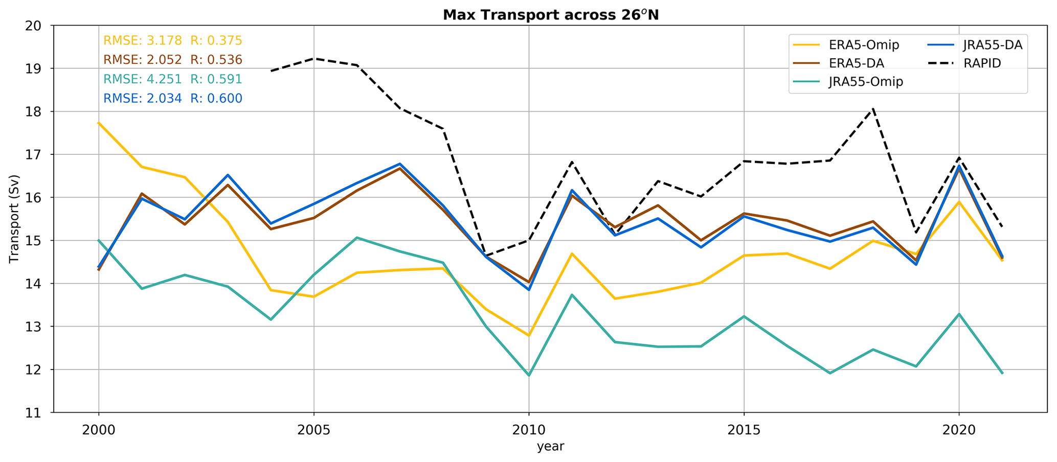
Figure 5 Maximum transport at 26.5° N from model output compared to the observations from the RAPID array.

Figure 6 Meridional volume streamfunction for the Atlantic, Pacific, and Southern oceans for ERA5 simulations. The third column shows the differences between DA and OMIP.

To verify that large-scale circulation is indeed improved when using data assimilation, we compare the maximum transport at 26° N in the Atlantic Ocean with the measurements taken by the RAPID array as a proxy for the strength of the Atlantic meridional overturning circulation (AMOC; Fig. 5). Again, we observe how data assimilation is associated with a reduced distance with respect to the observational reference. The OMIP simulations are characterized by low AMOC values that are strengthened when using data assimilation. This is confirmed by looking at the meridional volume streamfunction for different ocean sectors (Figs. 6 and 7). We see an increased and deeper transport in the Atlantic Ocean in both simulations when applying data assimilation. In addition, in the Southern Ocean transport is increased along the pathway of mode and intermediate-water formations between 50–45° S, pointing to an increased ventilation up to 1000 m depth. In the northern Pacific, intermediate-depth ventilation also seems to increase with a peak at around 40° N. In the deep ocean below 2000 m depth, the lower limb of the meridional overturning circulation is also strengthened in the Southern Ocean, in the whole Pacific Ocean, and (albeit less markedly) in the Atlantic Ocean.

Figure 7 The same as Fig. 6 but for JRA55.

Figure 8 Zonal averages of the idealized age tracer for the Atlantic, Pacific, and Indian oceans. The panels shows the differences in the last 20-year average between DA and OMIP simulations for ERA5 (a, c, e, g) and JRA55 (b, d, f, h).

As a result of these changes in global circulation, the ideal age tracer also shows consistent changes, where younger water penetrates deeper in the northern Atlantic Ocean, Southern Ocean, and northern Pacific Ocean (Fig. 8). At the same time, water age increases in the upper 1500 m of the subtropical gyres, while there is a general increased ventilation in the deep ocean below 2000 m, particularly in the Pacific Ocean. Important differences can be observed in the Atlantic Ocean between ERA5 and JRA55, as the penetration of younger waters in ERA5 is restricted to mainly between 1000–2000 m depth, while for JRA55 the increased ventilation seems to extend deeper to below 3000 m depth.

We also evaluated the effect data assimilation has on mixed-layer depth (MLD), an important metric for mass and energy exchanges between the atmosphere and the ocean. In this case, we use the climatology from de Boyer Montégut et al. (2004) as a reference. In Fig. 9 we can see how the bias is reduced in DA simulations with respect to the OMIP ones. This is particularly true in regions that are important hotspots of CO₂ exchange between the ocean and the atmosphere. For example, a deep bias is reduced in the northern Atlantic for ERA5, while for JRA55 the bias reduction goes in the opposite direction, i.e., towards correcting a shallow bias. In the Southern Ocean a shallow bias is clearly reduced in the Pacific and Atlantic sectors for ERA5, while the changes for JRA55 are less evident.

Figure 9 Yearly climatological (1970–2021) mean of mixed-layer depth. The four maps show the difference between each simulation and the observation-based gridded product from de Boyer Montégut et al. (2004). Annual and seasonal average RMSE values are reported above and below each map, respectively.

Figure 10 Differences between DA and OMIP simulations for DICant in the year 2021 for ERA5 (a, c, e, g) and JRA55 (b, d, f, h) at 500 m depth (a, b) and 2000 m depth (g, h).

To better understand the reasons for the differences in CO₂ uptake between OMIP and DA simulations, we have looked at the distribution of DIC_ant and the respective differences in the accumulation within the ocean interior (Fig. 10). Overall, when applying DA, we can see how DIC_ant decreases in the shallow water of the subtropical gyres, whereas there is a generalized increase in DIC_ant at high latitudes, even in shallow waters. In particular, the regions that show the largest increases in DIC_ant are the northern Atlantic Ocean and the Southern Ocean, where the increase is also visible at 2000 m depth. In the meridional sections in Fig. 11, we can observe the increase in DIC_ant in the formation region of intermediate and mode waters in the Southern Ocean, particularly in the Pacific and Atlantic sectors, and the increase in the deep northern Atlantic associated with an increase in AMOC. Here, consistent with the behavior of the age tracer, there is an important difference between ERA5 and JRA55, with the former showing a decrease in DIC_ant located below 2500 m depth and the latter a marked increase.

Figure 11 Differences between DA and OMIP simulations for DICant in the year 2021 for ERA5 (a, c, e, g) and JRA55 (b, d, f, h). The panels show zonal averages for the Atlantic, Pacific, and Indian oceans.

Figure 12 Differences between ERA5 simulations and GLODAP estimate for DICant in the year 2002. Zonal averages are shown for the Atlantic, Pacific, and Indian oceans.

We have also compared the distribution of DIC_ant with the estimate from GLODAP (Figs. 12 and 13). Here we can see how the negative bias with respect to the observation-based reference is reduced when applying data assimilation in both ERA5 and JRA55. This is particularly true for the Southern Ocean, where increased ventilation allows for a deeper penetration of DIC_ant. Overall, there is a reduction in RMSE when applying data assimilation (−10.2 % for ERA5 and −7 % for JRA55).

Figure 13 Differences between JRA55 simulations and GLODAP estimate for DICant in the year 2002. Zonal averages are shown for the Atlantic, Pacific, and Indian oceans.

Figure 14 Globally averaged SST from the four simulations compared with NOAA-ERSST_v5, IAPv4, and EN4.2.2.

For completeness, we have evaluated the impact of data assimilation on sea surface temperature (SST) using observation-based products different from those used for the data assimilation itself (see Table 2). Although we note that all SST products must share the majority of the observations on which they are based and therefore cannot be considered completely independent of one other, we use this exercise to once more assess whether the data assimilation is pushing the model's solution towards the observed state in a consistent way between the two different atmospheric forcings. Here we consider three products, and in all cases data assimilation is closer to these estimates than the OMIP simulations, particularly after 1990 (Fig. 14).

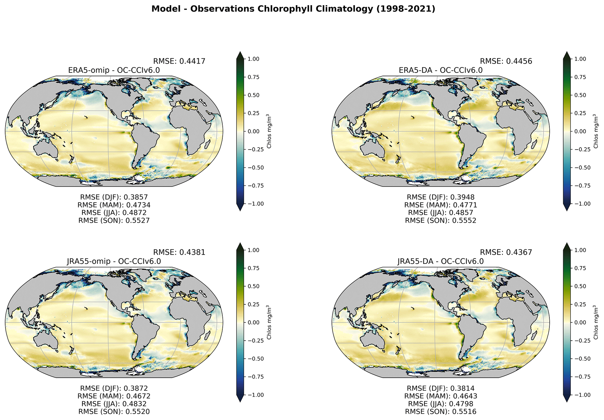
Figure 15 Yearly climatological (1998–2021) mean of surface chlorophyll. The four maps show the difference between each simulation and the OC-CCIv6.0 product. Annual and seasonal average RMSE values are reported above and below each map, respectively.

To complete our evaluation, we also compared surface chlorophyll produced by our simulations with the OC-CCIv6.0 dataset (Fig. 15). Similar to what was done for mixed-layer depth, we show the difference between the models and observations using a yearly climatology. In this case, we can observe how the effect of data assimilation is negligible overall, except in a narrow band between 30–40° N in both the northern Atlantic and the northern Pacific where the bias is actually slightly increased.

4 Discussion

We have compared two pairs of simulations performed with different atmospheric forcing reanalysis to evaluate the impact of assimilating observations of temperature and salinity on the overall representation of ocean biogeochemistry. The evaluation of CO₂ fluxes is problematic because there is no accepted observation-based product to be used as a single benchmark. All of the existing estimates begin from the same surface pCO₂ dataset, and each uses its own method to fill the blanks. We have shown that data assimilation consistently produces estimates of CO₂ fluxes that are better aligned with the central estimate of the Global Carbon Budget 2022 than their OMIP counterpart. However, the estimate of the GCB2022 is a combination of observation-based products and OMIP-type simulations performed with a suite of ocean biogeochemical models. This means that only atmospheric forcing is provided as a surface boundary condition to the ocean model and that no data assimilation is done. For this reason, showing that our estimates produced with data assimilation correlate better with the GCB22 estimate is informative but not enough to determine with confidence whether one practice (DA) is better than the other (OMIP).

For the above reasons, we decided to evaluate the performance of our simulations using the most comprehensive observational datasets available for several biogeochemical variables. When evaluating our simulations directly against the in situ observations of pCO₂, we observed a consistent improvement when applying data assimilation. Similarly, for other biogeochemical variables the evaluation gives consistent results going in the same direction. It is important to remember that no direct data assimilation is provided for these variables, and the degree to which they are impacted by the representation of the physical state of the ocean varies depending on the variable.

The distribution of macronutrients (nitrate, phosphate, and silicate) is controlled by large-scale three-dimensional circulation (e.g., MOC), vertical mixing (e.g., MLD), and primary productivity at the surface (e.g., chlorophyll here is used as a proxy for phytoplankton biomass). The same considerations apply to surface pCO₂ and related CO₂ fluxes because these are impacted by the large-scale distribution of both DIC and Alk, by vertical mixing, and in some regions by primary productivity. The same is true for oxygen as intermediate- and deep-water ventilation, together with vertical mixing, represent the main input of this gas into the interior of the ocean. However, the solubility of both O₂ and CO₂ is strongly dependent on temperature, and thus the data assimilation of this variable is likely to have a positive direct impact in their representation.

Based on these considerations, it is reasonable to assume that an improvement in the representation of the large-scale circulation is the main reason for an improved distribution between the upper and lower layers of all the tracers considered here. We have shown how data assimilation led to AMOC values that are closer to observations with respect to the OMIP simulations. This result is in line with Karspeck et al. (2017), who also found that subsurface constraints resulted in a greater AMOC mean strength and enhanced variance with respect to reference simulations with no data assimilation. The changes observed in the meridional volume streamfunction in the Southern Ocean, northern Atlantic Ocean, and northern Pacific Ocean, together with the changes observed in the distribution of the ideal age tracer, all point to a more ventilated ocean, which in turn has direct consequences in the distribution of biogeochemical tracers like oxygen and nutrients.

The improvement observed in the representation of the MLD is due to the ameliorated density profile obtained with data assimilation because the wind stress does not change between OMIP and DA simulations. The MLD can have a significant impact on the flux of CO₂, especially in those regions where we observed a bias reduction in the MLD itself. This impact becomes evident in the northern Atlantic, where we observe marked changes in the penetration of DIC_ant when applying data assimilation. Since the target observation dataset used for assimilating temperature and salinity in the ocean interior is the same between ERA5 and JRA55 (see Table 1), the resulting AMOC is rather similar in the two DA simulations due to the dominance of the resulting thermohaline structure (see Figs. 6 and 7, upper row) over other factors (e.g., atmospheric forcing). However, the changes in DIC_ant distribution caused by DA are different between ERA5 and JRA55 (see Fig. 11). This is due to a different response of the MLD over this region, where data assimilation causes MLD to deepen in the case of JRA55 and to shoal in the case of ERA5. This difference results in a deeper penetration of DIC_ant for JRA55-DA than for ERA5-DA with respect to their OMIP counterparts. However, it is important to note that the resulting DIC_ant distribution in this region is rather similar between ERA5-DA and JRA55-DA because these simulations share a very similar AMOC and a MLD that gets closer to observations from opposite ends.

We acknowledge that the global thermohaline structure resulting from assimilating temperature and salinity in the interior of the ocean strongly depends on the observation-based product used. Each product comes with its own problems and advantages. The product used here, EN4.2.2, displays a higher error variance than climatology for some regions, while at depth there is evidence that the climatological error variance is underestimated (Good et al., 2013). The decision to use this specific product was the result of a thorough analysis, trial-and-error attempts, and testing other products to obtain a robust reconstruction that could provide initial conditions for near-term climate predictions (Bilbao et al., 2021). The same reasoning applies to our choices of dataset for surface restoring of temperature and salinity, which were guided by the necessity of making sure that both SST and SSS fields were physically consistent with each other and with the atmospheric forcing applied. This exercise is repeated periodically with the objective of continuously improving the seasonal-to-decadal predictive system, and thus in the future using a different or improved dataset could lead to further improvement in the representation of ocean biogeochemistry.

Overall, data assimilation results in a more ventilated ocean and consequently a deeper penetration of DIC_ant in the interior of the ocean below the thermocline. Considering the comparison with the estimate of DIC_ant based on observations, this increase in DIC_ant in the deep ocean seems to be a change in the right direction. However, similar to what occurs for CO₂ fluxes, estimates of DIC_ant suffer from great uncertainty because the concentration of DIC_ant cannot be measured directly and must be derived using a variety of methods (Khatiwala et al., 2013). Still, for all variables considered so far there is a strong indication of a general improvement in their representation when applying data assimilation of temperature and salinity.

Certainly more difficult to explain is the limited response of surface chlorophyll despite an overall better representation of nutrients distribution and MLD. In fact, both nutrient availability and MLD have a direct impact on primary production and therefore on surface chlorophyll concentration. It is often the case that the default parameter set in an ocean biogeochemical model is chosen to reasonably reproduce both the large-scale distribution of nutrients and that of surface chlorophyll. In this study, the default configuration of PISCESv2 (Aumont et al., 2015) was used without any further adjustment of parameters. Because of the improvement in the large-scale distribution of nutrients and in their input into the productive layer, related to more realistic MLD, the model is presented with a different nutrient availability when applying data assimilation with respect to the OMIP simulations. Similarly, the average light exposure of phytoplankton changes with changes in MLD. In some regions, the bias in the chlorophyll surface fields is actually increased with data assimilation. This is the case for the northern Atlantic and northern Pacific regions, where a shallower MLD seems to coincide with an increase in surface chlorophyll between 30–40° N. In these regions, the model responds by increasing the distance with respect to the reference chlorophyll observations because the parameter set used was somehow selected to reproduce the same chlorophyll fields under different nutrient and light availability conditions. In the rest of the ocean, the chlorophyll field seems rather insensitive to the changes brought by data assimilation. For some regions, this is likely due to upper oligotrophic waters experiencing changes in nutrient input that are too little to significantly impact primary production. For regions with higher surface chlorophyll, like the equatorial Pacific Ocean and the Southern Ocean, the weak response is probably due to the availability of iron not changing significantly with the changes in circulation and MLD. In fact, a significant part of iron input in these regions is from atmospheric deposition that is left unchanged in all simulations.

5 Conclusions

We conclude that the assimilation of observations for temperature and salinity has a beneficial effect in the representation of large-scale circulation and mixed-layer depth, and this in turn translates into an improved representation of most of the ocean biogeochemical variables evaluated. Additionally, in the case of CO₂ and O₂, the improvements are most likely also driven by the direct beneficial effect that an ameliorated temperature field has on the solubility of these gases. In general, data assimilation drives a more vigorous overturning circulation, resulting in a more ventilated deep ocean. Ventilation increases in regions that are important hotspots for CO₂ fluxes like the Southern Ocean, the northern Atlantic Ocean, and the northern Pacific Ocean. The higher CO₂ uptake with data assimilation determines an increase in DIC_ant in the interior of the ocean below the thermocline and a decrease in shallow waters, particularly in the subtropical gyres. This deeper distribution of DIC_ant with respect to OMIP simulations is in better agreement with an observation-based product for DIC_ant. Because of this overall beneficial effect on the representation of ocean biogeochemistry, we conclude that CO₂ fluxes are most likely improved as well, although their direct validation is not straightforward. We have shown how not all aspects of biogeochemistry are improved as the surface chlorophyll field's representation is actually rather insensitive or even degraded when using data assimilation. We attribute this result to the choice of parameters for the biogeochemical model that was also based on a realistic representation of surface chlorophyll as a reference. Because of this, we suggest that ocean biogeochemical models be fine-tuned using simulations that include some degree of data assimilation of the physical fields whenever possible. Finally, since simple data assimilation practices, like the one presented here, can be included in simulations at negligible computational cost, we recommend that efforts like the Global Carbon Budget take into account this type of simulation in the future.