Regionally optimized high-resolution input datasets enhance the representation of snow cover in CLM5

Land surface processes, crucial for exchanging carbon, nitrogen, water, and energy between the atmosphere and terrestrial Earth, significantly impact the climate system. Many of these processes vary considerably at small spatial and temporal scales, in particular in mountainous terrain and complex topography. To examine the impact of spatial resolution and representativeness of input data on modelled land surface processes, we conducted simulations using the Community Land Model 5 (CLM5) at different resolutions and based on a range of input datasets over the spatial extent of Switzerland. Using high-resolution meteorological forcing and land use data, we found that increased resolution substantially improved the representation of snow cover in CLM5 (up to 52 % enhancement), allowing CLM5 to closely match performance of a dedicated snow model. However, a simple lapse-rate-based temperature downscaling provided large positive effects on model performance, even if simulations were based on coarse-resolution forcing datasets only. Results demonstrate the need for resolutions higher than 0.25° for accurate snow simulations in topographically complex terrain. These findings have profound implications for climate impact studies. As improvements were observed across the cascade of dependencies in the land surface model, high spatial resolution and high-quality forcing data become necessary for accurately capturing the effects of a declining snow cover and consequent shifts in the vegetation period, particularly in mountainous regions. This study further highlights the utility of multi-resolution modelling experiments when aiming to improve representation of variables in land surface models. By embracing high-resolution modelling, we can enhance our understanding of the land surface and its response to climate change.

1 Introduction

The Earth's changing climate is causing profound alterations in ecosystems globally, with large impacts on ecological, hydrological, and climatological processes (IPCC, 2014, 2023). In the context of the climate system, land surface processes control the exchange of carbon, nitrogen, water, and energy between the atmosphere and terrestrial ecosystems, hence profoundly influencing contemporary and future climate dynamics (Ferguson et al., 2012; Dirmeyer et al., 2006; Seneviratne et al., 2006). Seasonal snow cover greatly impacts this complex interplay, as it plays a vital role in the Earth's energy balance and hydrological cycle (Flanner and Zender, 2005; Barnett et al., 2005). More specifically, snow's characteristic high reflectivity (Flanner et al., 2011) substantially modulates land surface albedo and energy balance, while its low thermal conductivity (Zhang, 2005) allows snow to act as an insulating blanket for soil and organisms. More generally, agricultural irrigation often heavily relies on snowmelt for food production (Qin et al., 2020), while more than one-sixth of the world's population is dependent on water from glaciers or snowmelt (Barnett et al., 2005), highlighting the importance of glaciers and snow for human water demand (Mankin et al., 2015; Pritchard, 2019).

Within the integrated Earth system, important interactions and feedback mechanisms exist between energy, water, and nutrient cycles. In seasonally snow-covered areas, the snowpack creates numerous such interactions: it influences the energy balance by modulating the exchange of heat and moisture between the land surface and the atmosphere (Thackeray et al., 2019). It influences the partitioning of energy fluxes, affecting the magnitudes of both sensible and latent heat fluxes (Male and Granger, 1981), which, in turn, regulate the transfer of energy and water vapour, shaping the local and regional climate patterns (Ban-Weiss et al., 2011). Moreover, the duration and extent of snow cover has direct implications for vegetation periods, which has the potential to impact gross primary production (GPP), a measure of vegetation's ability to convert solar energy into chemical energy (and carbon dioxide to organic matter) through photosynthesis (Slatyer et al., 2022). Therefore, the presence or absence of snow cover directly influences the availability of water and sunlight for plants, influencing the productivity and carbon cycling within terrestrial ecosystems and resulting in direct links between melt-out date and biomass production (Jonas et al., 2008).

The Global Climate Observing System (GCOS, https://gcos.wmo.int/, last access: 12 August 2024) has identified snow cover extent as an essential climate variable, which further underlines the importance of snow for monitoring climate change and the critical role it has in regulating the energy balance of the planet. In physically based models, the representation of seasonal snow and its evolution are usually based on mass and energy balance calculations. Representations of snowpack structure range from simple, one-layer approaches (Douville et al., 1995) to complex schemes that resolve up to 50 snowpack layers and track the evolution of their microstructural properties (Vionnet et al., 2012; Bartelt and Lehning, 2002). For model applications at large scales and coarse resolutions, snowpack representations with few (3 to ca. 10) layers (Essery et al., 2013; Niu et al., 2011) have been found to be an adequate compromise between model complexity and accuracy (Dutra et al., 2012; Magnusson et al., 2015).

Land surface models (LSMs) specifically target global-scale applications, as they were initially developed to represent the lower atmospheric boundary condition of global circulation models. Land surface modelling has seen remarkable progress in recent years, evolving from simple biophysical parameterizations to complex frameworks that incorporate key processes such as soil moisture dynamics, land surface heterogeneity, and plant and soil carbon cycling (Fisher and Koven, 2020; Lawrence et al., 2019). Today's LSMs are thus principally suitable for, and even intended to, study process interactions and feedbacks within the Earth's systems (e.g. Lawrence et al., 2019). However, large challenges in land surface modelling today remain due to uncertainties in process representation, unresolved sub-grid heterogeneity, and the projection of spatial and temporal dynamics of model parameters (Beven and Cloke, 2012; Fisher and Koven, 2020; Fisher et al., 2019; Blyth et al., 2021). It is these limitations that make it difficult to reconcile site-scale experimental data and LSM simulations, hampering their evaluation and further development. Multi-resolution modelling setups (including the point and site scale) overcome this very limitation (e.g. Singh et al., 2015; Meissner et al., 2009), as they allow evaluating a spatially distributed LSM simulation over a large spatial extent, while at the same time certain aspects of the model (i.e. snow depth or snow cover duration) can be validated at the point scale using in situ observations. This is especially of value if meteorological forcing data (e.g. station data), land use information, and model evaluation data are available for a specific point-location.

Today, a strong push is evident towards higher-resolution modelling, such as 1 km simulations (Schär et al., 2020). While achieving this level of resolution globally over extended periods remains a challenge due to computational limitations, higher resolution allows for a more precise representation of land surface heterogeneity, which directly influences the representation of various key parameters and their associated processes (e.g. Ma and Wang, 2022; Rimal et al., 2019; Zhang et al., 2017). Because depth, duration, and variability of seasonal snow cover is strongly affected by topography and thus highly variable in space (e.g. Clark et al., 2011), higher resolution enables a more detailed characterization of snow distribution, depth, and duration, capturing the spatial variability of snow cover across diverse landscapes (Lei et al., 2022; Magnusson et al., 2019; Essery, 2003). Improved representation of snow cover dynamics has the potential to enhance simulation of surface albedo, which affects the amount of solar radiation reflected back into the atmosphere, and thus influences the overall simulated surface energy balance (Thackeray and Fletcher, 2016; Flanner et al., 2011). An improved representation of snow melt-out date can further directly affect simulations of land surface phenology (Xie et al., 2020).

In this study, we explore how model resolution and the quality of meteorological and land surface datasets affect the representation of seasonal snow cover dynamics in the Community Land Model 5 (CLM5), a state-of-the-art LSM. More specifically and based on the ideas highlighted above, we hypothesize that with increasing spatial resolution and quality of meteorological and land surface input datasets, the representation of snow cover dynamics and its associated variables in CLM5 can achieve an accuracy comparable to that of a dedicated snow model.

To test this hypothesis, we implement a multi-resolution modelling framework using CLM5. This framework bridges the gap between the point and site scale and spatially distributed land surface modelling, thus allowing us to compare model accuracy across a hierarchy of spatial scales and using diverse evaluation data, while preserving model architecture. As a result, confounding effects due to differences in process parameterizations are eliminated, isolating and clarifying the effects of model resolution and input data and allowing us to assess the importance of an accurate representation of sub-grid variability within coarser-resolution models.

We apply our framework to the spatial extent of Switzerland, including relevant watersheds of neighbouring countries. This region provides an ideal setting due to its diverse topography, encompassing both the Swiss Alps and the Swiss plateau. Through a set of modelling experiments, we assess the relative impact of detailed meteorological and land cover information on snow simulations with CLM5 across topographically complex landscapes. Our findings can inform the optimal design of further offline applications of LSMs, for instance (1) to extrapolate local-scale experimental findings; (2) to address the limitations of global-scale, coarse-resolution simulations; and (3) to support the interpretation of snow cover information contained in Earth system simulations.

2 Methodology

2.1 Land surface modelling

To investigate the effects of spatial resolution and input datasets in LSMs, we use the land component of the Community Earth System Model (CLM5), an open-source, state-of-the-art, and widely used LSM that simulates carbon, nitrogen, water, and energy exchange between the atmosphere and the land surface (Lawrence et al., 2019, 2018). It offers two operational modes: prognostic biogeochemistry (BGC) mode and prescribed satellite phenology (SP) mode. For this study, we focused on running CLM5 in SP mode, where remote sensing-based datasets are used to prescribe spatial extents of plant functional types (PFTs), crop functional types (CFTs), and the PFT-specific monthly plant area index (PAI, sum of leaf area index and stem area index), hence reducing the degrees of freedom compared to prognostic calculations. See Sect. 2.3.2 for more information.

It is important to note that in SP mode, carbon–nitrogen cycling is not considered, and certain processes such as leaf nutrient limitation and respiration terms are omitted. GPP for the context of this study was approximated by photosynthetic activity, with photosynthesis being limited by carboxylation, light, and export limitations for different plant functional types (Thornton and Zimmermann, 2007; Farquhar et al., 1980). The photosynthesis module in CLM5 is described in detail by Thornton and Zimmermann (2007), Bonan et al. (2011), and Oleson et al. (2010). Simulations were performed with the Leaf Use of Nitrogen for Assimilation (LUNA) routine turned on (Ali et al., 2016). Evapotranspiration in CLM5 is calculated as the sum of transpiration, evaporation (considering soil and snow evaporation, ice and snow sublimation, and dew), and canopy evaporation following Lawrence et al. (2007).

Spatial resolution influences the representation of spatial heterogeneity in CLM5, which is represented by a sub-grid hierarchical system. Each grid cell is split into different land units (vegetation, glacier, lake, urban, crop). On the second sub-grid level (column level), potential variability in the soil and snow state variables within the same land unit is accounted for. However, the vegetation and lake land unit only allow for a single column. Each vegetated column can be further divided up into up to 15 PFTs or bare ground (this is the third sub-grid level in CLM5, often referred to as the patch level). Vegetation structure for each PFT is described by monthly varying leaf area index (LAI), stem area index (SAI), and canopy top and bottom heights. All of these values are prescribed in our model setup (satellite phenology mode).

Here, we applied CLM5 to both the regional scale and the point scale, for which CLM5 features a dedicated point mode (PTCLM). It is worth noting that what we refer to as point-scale simulations incorporate fractional state variables (e.g. fractional snow cover), as the gridded modelling algorithms (i.e. exactly the same as used for large-scale gridded simulations) are directly applied to a single point. From a snow cover modelling perspective such an approach would be referred to as site-scale simulation, but in order to be consistent with LSM conventions we refer to them as point-scale simulations. As there is no lateral exchange in our model setup (river routing is off), there is no difference in running a dedicated point simulation and taking out individual grid cells from a regional simulation, apart from the fact that we have additional information at these station locations (e.g. meteorological station data for forcing, exact GPS location for downscaling temperature). We elaborate on our experiment setup for point-scale and gridded simulations in Sect. 2.2.

2.1.1 Snow and fractional snow cover schemes in CLM5

Snow cover provides a convenient means of observing and validating the internal energy turnover of LSMs, and it is the duration of snow cover that influences vegetation periods, ecophysiological processes, and carbon cycles. The snow scheme in CLM5 classifies as a multi-layer snow model with detailed internal snow process schemes (Boone and Etchevers, 2001). General snow parameterizations are based on Anderson (1976), Jordan (1991), and Dai and Zeng (1997), with fractional snow cover calculations being based on the method of Swenson and Lawrence (2012). In recent years there have been several updates to the snow-related parameterizations, most notably an inclusion of wind and temperature effects on fresh snow density and an increase in maximum snow layers from 5 to 12 (Lawrence et al., 2019). A detailed description of snow related calculations in CLM5 can be found in Lawrence et al. (2018), but for convenience we also give a brief summary of snow-related parameterizations used in CLM5 here. In CLM5, a snowpack can be made up of up to 12 layers, with the lowest being at the snow–soil interface and the uppermost at the snow–atmosphere interface. Each layer is described by mass of water, mass of ice, layer thickness, and temperature. Any snowpack smaller than 10 cm is treated as a single layer and only described by mass of snow.

Upon falling of solid precipitation on a column, either a new snow layer is initialized (if >10 cm) or the snow is added to the present one, whereby combination and subdivision of snow layers is based on Jordan (1991). Mass of ice in each snow layer is calculated based on the rate of solid precipitation reaching the ground, taking into account gains due to frost, losses due to sublimation, and change in ice due to phase change (melting). Bulk density of newly fallen snow is calculated dependent on air temperature and further increased if wind speeds exceed 0.1 m s⁻¹ due to wind compaction, following van Kampenhout et al. (2017). CLM5 includes four processes leading to overall snow compaction: (1) destructive metamorphism of new snow, (2) snow load, (3) melting, and (4) drifting snow. Mass of water in each layer is dependent on liquid water flow in and out of the layer and change in liquid water due to phase change (melting). For the top snow layer this includes rate of liquid precipitation falling, evaporation, and liquid dew. Any water flowing out of the lowest snow layer contributes to surface runoff and infiltration calculations in different CLM5 subroutines.

An essential variable for the energy balance due to its effects on surface albedo is fractional snow-covered area (FSno). FSno is further of importance as CLM5 calculates surface energy fluxes separately for snow-free and snow-covered land unit fractions. FSno in CLM5 is calculated following Swenson and Lawrence (2012), which uses separate parameterizations for the snow accumulation and depletion phase. During accumulation, FSno is calculated as follows:

$$\begin{array}{}\text{(1)}& {\mathrm{FSno}}^{n+\mathrm{1}}=\mathrm{1}-\left(\right(\mathrm{1}-\tanh \left(\mathrm{0.1}{q}_{\mathrm{sno}}\mathrm{\Delta }t\right)\left)\right(\mathrm{1}-{\mathrm{FSno}}^n\left)\right),\end{array}$$

where q_snoΔt quantifies the amount of new snow. FSnoⁿ and FSnoⁿ⁺¹ denote FSno at the previous and current time step, respectively. During snowmelt, the following parameterization is used:

$$\begin{array}{}\text{(2)}& {\mathrm{FSno}}^{n+\mathrm{1}}=\mathrm{1}-{\left[{\displaystyle \frac{\mathrm{1}}{\mathit{\pi }}}\mathrm{acos}\left(\mathrm{2}{\displaystyle \frac{W}{W_{max}}}-\mathrm{1}\right)\right]}^{n_{\mathrm{melt}}}.\end{array}$$

W is the simulated snow water equivalent (SWE) at the current time step, and W_max is the maximum accumulated SWE of the snow season. n_melt is the snow-covered area shape function, which is determined from σ_topo, the standard deviation of topography within a grid cell, by

$$\begin{array}{}\text{(3)}& n_{\mathrm{melt}}={\displaystyle \frac{\mathrm{200}}{max(\mathrm{10},{\mathit{\sigma }}_{\mathrm{topo}})}}.\end{array}$$

2.1.2 Rain–snow partitioning in CLM5

CLM5 partitions total precipitation into rain and snow according to a linear temperature ramp, resulting in all snow below 0 °C, all rain above 2 °C, and a mix of rain and snow for intermediate temperatures. More specifically, the fraction of total precipitation P falling as rain (q_rain) and snow (q_snow) at each time step is calculated as follows:

$$\begin{array}{}\text{(4)}& {\displaystyle }{q}_{\mathrm{rain}}=P\left(f_p\right),\text{(5)}& {\displaystyle }{q}_{\mathrm{snow}}=P(\mathrm{1}-f_p),\text{(6)}& {\displaystyle }{f}_p=\mathrm{0}<\mathrm{0.5}(T_{\mathrm{atm}}-T_f)<\mathrm{1},\end{array}$$

where T_f is set to 0 °C.

2.2 Model experiments with CLM5

Figure 1 provides a general overview of the experimental setup, which includes three aspects. Firstly, we varied the spatial resolution, ranging from 0.5° (10×6 grid cells) to 0.25° (19×11 grid cells) to 1 km (365×272 grid cells) over the study domain. As the 0.5 and 0.25° grids were chosen to closely match the extent of the pre-determined 1 km grid, grid anchoring might slightly vary between resolutions. Secondly, we used different meteorological forcing datasets, including a globally available coarse-resolution dataset (Clim_CRU), the same global dataset with lapse-rate-corrected temperature (Clim${}_{{\text{CRU}}^{*}}$), and a high-resolution regional dataset (Clim_OSHD). Lastly, we considered two options for land use information: a global dataset (LU_Gl) and a high-resolution dataset (LU_HR). This approach is intended to cover the multiple facets of resolution: on the one hand, the spatial resolution of the CLM5 simulations themselves and, on the other hand, the “native” resolution (or level of detail) of the input datasets, with higher resolution implying better quality of the datasets. Different CLM5 configurations were set up to cover the variations in spatial resolution, meteorological forcing, and land use information.

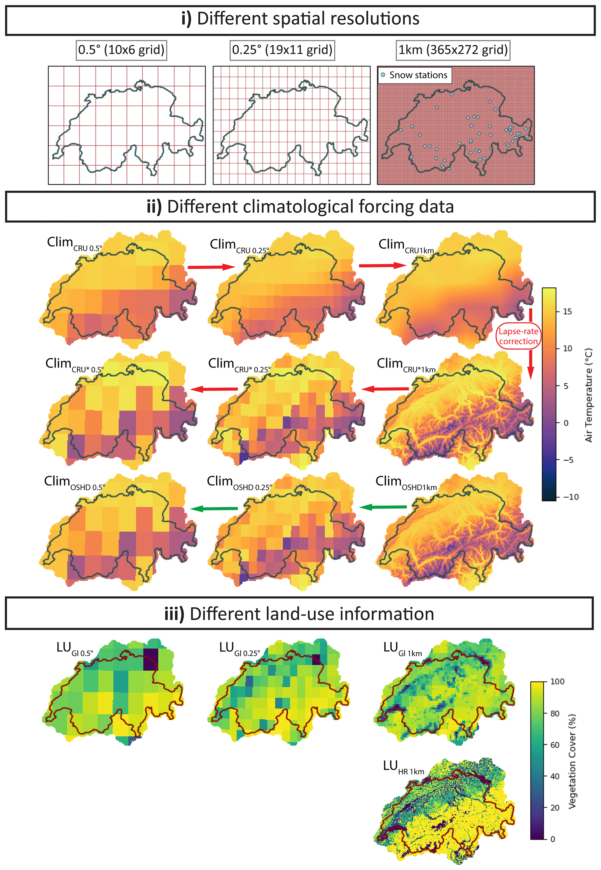
Figure 1 Schematic overview specifying the three facets of the experimental setup: variation of (i) spatial resolution, (ii) meteorological forcing data, and (iii) land use information. Panel (i) shows the different grids used, including the locations of the snow stations. Panel (ii) shows monthly mean temperature (May 2018) from the different data sources: a globally available coarse-scale dataset (Clim_CRU), the same but with a lapse-rate-corrected temperature (Clim${}_{{\text{CRU}}^{*}}$), and a high-resolution regional dataset (Clim_OSHD). Note that Clim_CRU data are provided at 0.5° (top-left most panel in ii) and bilinearly regridded to 0.25° and 1 km. Clim_CRU1 km is then downscaled via a lapse rate correction to obtain Clim${}_{{\text{CRU}}^{*}\mathrm{1}\mathrm{km}}$, before being upscaled to obtain Clim${}_{{\text{CRU}}^{*}\mathrm{0.25}\mathit{°}}$ and Clim${}_{{\text{CRU}}^{*}\mathrm{0.5}\mathit{°}}$. Apart from temperature, meteorological forcing data are identical for Clim_CRU1 km and Clim${}_{{\mathrm{CRU}}^{*}\mathrm{1}\mathrm{km}}$ simulations. Clim_OSHD data are provided at 1 km and upscaled to 0.25 and 0.5°. Panel (iii) shows differences in land use information considered in this study using the example of percentage vegetation cover (sum of vegetation PFTs and crop CFTs).

At the 1 km scale, CLM5 was run with six different configurations, each using different combinations of meteorological forcing and land use information. At the 0.5 and 0.25° resolutions, CLM5 was run with three configurations corresponding to the respective meteorological forcing datasets and using the global land use dataset. These regional CLM5 simulations across the spatial extent of Switzerland and adjacent watersheds of neighbouring countries, covering an area of 44 050 km², were set up in an identical way as global simulations.

Additionally, point-scale simulations were conducted at 36 snow-monitoring station locations within the model domain. At the snow monitoring stations, we focus on the impact of meteorological forcing and land surface input on CLM5 simulations by first running the same six configurations as for the 1 km gridded experiment. While exactly the same modelling framework was used for these point-scale simulations as for the gridded simulations, meteorological forcing was station specific (e.g. not just the extracted meteorological forcing from the closest 1 km grid cell; see Sect. 2.3.1 for additional information). Knowing that all 36 snow-monitoring stations are located on non-forested land, we set up three additional simulations enabling direct comparison of observations with respective simulations. For each meteorological forcing dataset (Clim_CRU, Clim${}_{{\text{CRU}}^{*}}$, Clim_OSHD), we set up a simulation where the land unit was set to be 100 % vegetated with PFT 0 (bare ground) rather than using the composite grid cell from the LU_HR and LU_Gl dataset, respectively. This additional land use dataset is further referred to as LU_nofor. Model performance evaluation was carried out based on in situ observations at these stations (see Sect. 2.4.1 and 2.5.1 for more information).

The performance of all gridded CLM5 configurations in simulating seasonal snow cover was assessed against simulations obtained with a dedicated snow model (see Sect. 2.4.2 and 2.5.2 for more information). Outcomes from the snow cover analyses were complemented by a relative comparison of the different gridded CLM5 configurations for the ecophysiological variables gross primary production and evapotranspiration.

2.3 Input datasets

Each CLM5 model configuration requires the following meteorological driving data: incident short- and long-wave radiation, air temperature, relative humidity, wind speed, pressure, and precipitation. Additionally, a land surface information file is required.

CLM5 simulations were set up to run between January 2016 and December 2019, in order to maximize the temporal overlap between the various meteorological forcing datasets and available data for model benchmarking. We further performed 10 years of spin-up by recycling through the available input data. A spin-up was necessary to ensure soil moisture and soil temperature were in approximate equilibrium and not affecting temporal dynamics and physical properties, e.g. of the simulated snow cover evolution.

2.3.1 Meteorological forcing

To assess the impact of meteorological input data quality, we considered three meteorological forcing datasets with increasing level of detail. As an example of a standard global dataset, we used the recent state-of-the-art dataset CRU-JRA (University of East Anglia Climatic Research Unit; University of East Anglia Climatic Research Unit and Harris, 2019), which provides near-global (excluding Antarctica) 6-hourly meteorological data on a 0.5° × 0.5° latitude–longitude grid. CRU-JRA is a merged product of the monthly Climate Research Unit (CRU) gridded climatology (Harris et al., 2014) with the Japanese Reanalysis product (JRA, Kobayashi et al., 2015). We selected CRU-JRA due to its large time span (1901–2020), which includes recent years and hence ensures sufficient overlap with our high-resolution forcing dataset (see below), as well as due to its application in the annual Global Carbon Budget assessments (e.g. TRENDY, Friedlingstein et al., 2020) and in the Land Surface, Snow and Soil Moisture Model Intercomparison Project (LS3MIP, van den Hurk et al., 2016). The original 0.5° CRU-JRA dataset was first projected to our model domain using nearest-neighbour techniques (Clim_CRU0.5°), before regridding it to 0.25°, 1 km, and all point locations using bilinear interpolation to obtain Clim_CRU0.25°, Clim_CRU1 km, and Clim${}_{{\text{CRU}}^{\mathrm{pt}}}$, respectively.

As a dataset representing an intermediate level of detail, we upgraded the Clim_CRU1 km and Clim${}_{{\text{CRU}}^{\mathrm{pt}}}$ datasets by downscaling temperature data using a temperature lapse rate of −6.5 K every 1000 m, which resulted in the Clim${}_{{\text{CRU}}^{*}}$ and the Clim${}_{{\text{CRU}}^{*\mathrm{pt}}}$ datasets. This approach was intended to account for variations in air temperature within the complex topography of the Swiss Alps and subsequent refinement of the partitioning of precipitation into snow and rain. We use a global DEM at 0.5° to first bring temperature to sea level temperatures by applying negative lapse rates, before using a high-resolution DEM of Switzerland to relapse temperature (see Fig. C1 in Appendix C for both DEMs). For the snow station locations we used the actual GPS measurement of each station, resulting in Clim${}_{{\text{CRU}}^{*\mathrm{pt}}}$. The updated 1 km fields were upscaled back to 0.25 and 0.5° to also inherit this correction in the coarser-resolution simulations. This resulted in the Clim${}_{{\text{CRU}}^{*}}$ dataset. All other forcing variables were left identical for the Clim_CRU1 km, Clim${}_{{\text{CRU}}^{*}\text{1\hspace{0.17em}km}}$, Clim${}_{{\text{CRU}}^{\mathrm{pt}}}$, and Clim${}_{{\text{CRU}}^{*\mathrm{pt}}}$ simulations.

As the input datasets with the highest level of detail, we used meteorological forcing generated according to methods developed by the Operational Snow Hydrological Service (OSHD) at 1 km spatial and 1 h temporal resolution and all point locations at 1 h temporal resolution. Necessary meteorological input variables were all provided by MeteoSwiss (COSMO1 and COSMOE product), and specific downscaling routines were applied, e.g. to incoming solar radiation and wind velocity to optimally capture the influence of complex topography. Of particular relevance to this study is the correction of snowfall input fields by assimilation of station data according to Magnusson et al. (2014). In the context of this study, this dataset can be considered a meteorological input specifically optimized for accurate gridded snow cover simulations. The 1 km forcing data were then upscaled to the desired target resolution (0.25 and 0.5°) with no smoothing applied. We refer to Mott et al. (2023) for further details with regard to the Clim_OSHD product. The OSHD downscaling algorithms were also applied for each specific snow station location, resulting in the Clim${}_{{\text{OSHD}}^{\mathrm{pt}}}$ dataset for the point-scale simulations.

2.3.2 Land use information

Global-scale land use information

Input datasets for the land surface are based on the global-scale input dataset commonly used in CLM5, where extents of each land unit and percent plant functional type for each grid cell are derived from MODIS satellite data (Lawrence and Chase, 2007), as are monthly LAI and SAI values. In a first step, which was performed separately for each target resolution (including all point locations), we used the standard CLM tools (including the Earth System Modelling Framework (ESMF) regridding tools), to obtain our “global info” land surface dataset (LU_Gl; see Fig. 1). This represents a land surface dataset equivalent to that which would be used in a typical large-scale LSM or general circulation model application. Note that the resolution of the underlying global datasets varied (0.05° for urban, lake, or glacier datasets and 0.25° for vegetated, PFT fraction, LAI, and SAI datasets), since we used the most commonly applied CLM5 datasets. This step resulted in the LU_Gl0.5°, LU_Gl0.25°, and LU_Gl1 km datasets (see Fig. 1). In Appendix B we show obtained land unit distributions per grid cell for all three target resolutions (Figs. B2, B3, and B4 for LU_Gl1 km, LU_Gl0.25°, and LU_Gl0.5°, respectively) and patch-level PFT distributions (Figs. B6, B7, B8) and monthly PAI for temperate needle-leaf evergreen trees (Figs. B10, B11, B12) and boreal broadleaf deciduous trees (Figs. B14, B15, B16).

High-resolution land use information

To obtain an alternative land use input dataset (LU_HR1 km) with a higher level of detail and based on a more up-to-date land use dataset, the LU_Gl1 km dataset was updated based on a combination of high-resolution data sources: (1) Copernicus Global Land Service PROBA-V data (2) Copernicus Sentinel-3/OLCI data, and (3) high-resolution national forest mixing ratios derived specifically for Switzerland (100 m resolution, Swiss-Federal-Statistical-Office, 2013). In a first step, land unit distributions per grid cell (first sub-grid level in CLM5) were computed using the Copernicus PROBA-V 100 m 2019 land cover datasets, which have been shown to be of high spatiotemporal quality (e.g. 79.9 % accuracy over Europe for the discrete classification dataset, Tsendbazar et al., 2021). The native 100 m fractional cover datasets were reprojected and regridded to our domain using ESMF tools (with a bilinear interpolation algorithm). We used the Copernicus built-up cover fraction to obtain the spatial extent of the urban land unit (assumed to be all at medium density), the crop cover fraction for the crop land unit (assumed to all be rainfed, non-irrigated land), and the level 1 discrete classification dataset for lake and glacier land units. The vegetated land unit was derived by adding Copernicus PROBA-V grass cover fraction, tree cover fraction, shrub cover fraction, and bare cover fraction together. Minor adjustments were necessary due to regridding artefacts to ensure (i) no pixel exceeded 100 % (e.g. around edges of lakes) and (ii) each pixel added up exactly to 100 % (any non-classified pixels were classified as non-vegetated). Figure B1 shows the extent of the LU_HR1 km dataset for each CLM5 land unit.

For the third sub-grid level (patch level) of the vegetated land unit, we merged the 100 m Copernicus forest type layer and the 100 m Copernicus shrub and grass cover fraction with the Swiss national 100 m forest mixing ratio data. The Copernicus forest type layer distinguishes between six forest classes (needle-leaf and broadleaf evergreen forests, needle-leaf and broadleaf deciduous forests, mixed forests, and unclassified areas) which were translated to CLM5 PFTs in the following manner: evergreen trees (both deciduous and broadleaf) were classified as needle-leaf evergreen temperate trees (PFT2), deciduous needle-leaf trees were classified as needle-leaf deciduous boreal trees (PFT4), and deciduous broadleaf trees were classified as broadleaf deciduous temperate trees (PFT8). All shrubs from Copernicus shrub cover were assumed to be broadleaf deciduous shrubs (PFT12), and all grass and sparsely vegetated cells were classified as C₃ grass. Mixed and unknown pixels were then updated based on the Switzerland-wide dataset. If the Swiss dataset classified it as needle-leaf forest, it was set to PFT2, whereas if it was a deciduous forest, it was PFT 8. Needle-mixed and deciduous-mixed forest were set to PFT 4, while no wood was classified as C₃ grass (PFT 13). Figure B5 shows the percentage PFT fractions of the LU_HR1 km dataset.

In order to obtain an updated LAI dataset, Copernicus Sentinel-3/OLCI/PROBA-V data at 333 m spatial resolution were used, which have a temporal resolution of three time steps per month. We used data for the year 2020, and averaged the 3-monthly time steps to obtain one layer of LAI data per month. For evergreen PFTs, August LAI was used year-round, whereas for deciduous PFTs the respective monthly values were used. LAI of pixels where satellite data were not available (snow, clouds) was set to 1. LAIs of crops, shrubs, and grasses remained unchanged in the LU_HR1 km dataset. Figures B9 and B13 show monthly PAI for temperate needle-leaf evergreen trees (PFT2) and boreal broadleaf deciduous tree (PFT 4).

2.4 Test datasets

We used two datasets to assess model performance. The first, consisting of daily snow depth observations from 36 snow stations, allowed us to evaluate the performance of CLM5 point-scale configurations in simulating seasonal snow cover against ground truth data. For an evaluation of the gridded CLM5 simulations, we employed the Flexible Snow Model (FSM2) as a reference snow model for validation.

2.4.1 Snow stations

The 36 snow stations considered cover an elevational gradient, are spread throughout Switzerland (see Fig. 1), and were selected from an exceptionally dense and accurate network of snow observations. Table A1 in Appendix A specifies the locations and characteristics of each of these sites. Observations at the station locations consist of daily monitored snow depth (HS), which are collected as part of the snow monitoring networks of either the WSL Institute for Snow and Avalanche Research (SLF) or the Federal Office for Meteorology and Climatology (MeteoSwiss). HS measurements were extracted at a daily time step and cleaned from obvious outliers (assessed against neighbouring stations at similar elevations), which can occur, e.g. due to measurement errors (see Mott et al., 2023, for more details).

2.4.2 Snow cover simulations with FSM2

The Flexible Snow Model (FSM2, Mazzotti et al., 2020), a recent upgrade of the Factorial Snow Model (FSM, Essery, 2015), is an open-source, physics-based snow model of intermediate complexity. As in CLM5, FSM2 represents the snowpack with few layers only (up to three in the version used here), where each layer is characterized in terms of mass of water, mass of ice, layer thickness, and temperature. Snow cover processes in FSM2 include heat conduction through the snowpack, transport (and refreezing) of liquid water in the snowpack, the evolution of snow density by compaction, and surface albedo. For further detail on the parameterizations of snow properties and processes, we refer to Essery (2015) and Mott et al. (2023). Contrary to CLM5, FSM2 does not include a precipitation partitioning scheme but accepts separate inputs of solid and liquid components. Precipitation partitioning is performed offline following a sigmoid function centred around 1.04 °C and based on the 10 m air temperature (Ta_10 m, in °C):

$$\begin{array}{}\text{(7)}& {\displaystyle \frac{\mathrm{snowfall}}{{\mathrm{precip}}_{\mathrm{tot}}}}={\displaystyle \frac{\mathrm{1}}{\mathrm{1}+\exp \left(\frac{{\mathrm{Ta}}_{\mathrm{10}\mathrm{m}}-\mathrm{1.04}}{\mathrm{0.15}}\right)}}.\end{array}$$

Simulations at 250 m resolution and point simulations at snow station locations have been specifically set up and calibrated by SLF to run over the extent of Switzerland for the purpose of operational snow water resources monitoring (Griessinger et al., 2019; Mott et al., 2023). At the 250 m resolution, model grid cells are subdivided into forest, open, and glacier fractions, with forest cover descriptors derived from a 1 m resolution, lidar-based canopy height model available for Switzerland (Mott et al., 2023; Waser et al., 2017). Snow cover fraction parameterizations differ for each tile; for details we refer readers to Sect. 2.1.2 in Mott et al. (2023). In the absence of high-quality, spatially distributed snow depth observations over the entire extent of Switzerland, these FSM2 simulations served as ground truth for this study. For comparison with CLM5 output, 250 m resolution FSM2 output results were upscaled to 1 km without smoothing (e.g. conservative regridding).

2.5 Evaluation of model experiments

2.5.1 Comparing point-scale CLM5 model simulations to station observations of snow depth

Observations at the snow monitoring stations (Fig. 1 and Table A1) provide an exceptional opportunity to allow proper assessment of regional model performance. Sub-sampled from a dense, high-quality network of snow observations, these measurements of snow height were used to assess the ability of each station-specific point-scale CLM5 configuration to simulate seasonal snowpack in Switzerland and were additionally compared to FSM2 simulations. The evaluation of FSM2 runs allowed us to assess whether FSM2 is a suitable model to be used as a reference for the gridded simulations.

The stations were binned into three elevational bands (<1000, 1000–2000, >2000 m a.s.l.) resulting in 10, 12, and 14 stations for the low-, mid- and high-elevation band, respectively. For each station location, the various CLM5 point-scale simulations (Clim_CRU1 km + LU_{Gl/HR 1 km}, Clim${}_{{\text{CRU}}^{*}\mathrm{1}\mathrm{km}}$ + LU_{Gl/HR 1 km}, Clim_OSHD1 km + LU_{Gl/HR 1 km}) and the FSM2 simulation were compared to observations of snow depth (HS) by computing relative and absolute differences and root-mean-square errors (RMSE) and Mean absolute errors (MAE) for the time frame between October and July across all four simulated snow seasons.

Additionally, we use wiggle plots to show the seasonal evolution of model errors for all the point-scale simulations across the 2017/18 season.

2.5.2 Comparing gridded CLM5 model simulations to FSM2 simulations of snow depth

Given that the point-scale evaluation against station data offers an incomplete picture of CLM5 performance in its “typical” setting (coarse resolution, gridded) as it is limited to point locations with a narrow range of topographic and vegetation characteristics, we provide a complementary evaluation of all gridded CLM5 simulations against FSM2. This model evaluation was performed at 0.25° resolution, which is a fair target given the complexity of the topography across our modelling domain and its relatively small size and considering today's ever-increasing computational resources. FSM2 and 1 km CLM5 simulation results were hence upscaled to 0.25° using a conservative upscaling approach, which preserves areal averages. For this purpose, we had to decrease our evaluation domain slightly, as we performed the 1 km simulations with a mask running exactly along the edges of our modelling domain, making it impossible to upscale these areas to 0.25° without crude assumptions. The 0.5° simulations were downscaled to 0.25°, and all simulations were evaluated across the same domain.

For the evaluation and quantification of snow-related CLM5 model experiment performance we used a Taylor diagram (Taylor, 2001), with FSM2 simulations of snow depth at 0.25° as our reference. A Taylor diagram combines centred RMSE, correlation coefficients, the spatial and temporal standard deviation, and hence it describes overestimation or underestimation of the models relative to a benchmark.

Additionally, in order to better understand patterns in model discrepancy as they relate to topography and land cover, we compared simulated snow depth (HS) as a function of elevation for three dates during the 2018/19 winter season (early winter 1 December, mid winter 1 February, late winter 1 April). This comparison was performed at 1 km and only included the six 1 km CLM5 simulations and FSM2, hence no up- or down-sampling was necessary, and the effect of elevation could be assessed over a larger distribution. We further compared changes in land use information and simulated snow cover for non-forested vs. forest-dominated grid cells, allowing an assessment of whether the sensitivity to the chosen dataset depends on the land cover type.

3 Results

3.1 Evaluation of snow simulations at point locations

We begin by focusing on simulated snow depth at point locations. We observed distinct differences in performance using different meteorological forcing datasets in our CLM5 experiments (see Fig. 2). The point-scale CLM5 model using global meteorological forcing data (Clim${}_{{\text{CRU}}^{\mathrm{pt}}}$ + LU_Gl/HR/nofor) showed poor performance in modelling seasonal snow development across all snow station locations. RMSEs were close to 1 m for mid-elevation stations and only marginally better for high- and low-elevation stations. This demonstrates that these runs fail to accurately represent elevational gradients in temperature and snow amounts, making the error dependent on how closely the characteristics of the station happen to match the characteristics of the coarse-resolution grid cells of the Clim_CRU forcing dataset.

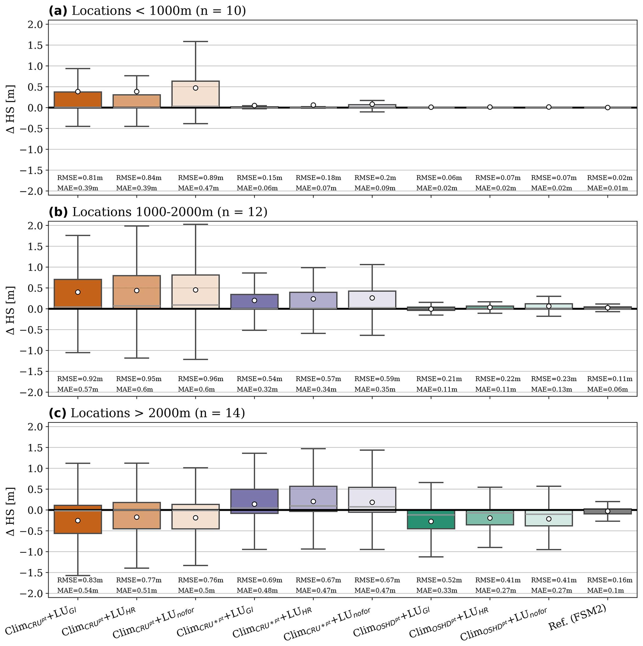
Figure 2 Comparisons of point-scale model simulations to observations of snow depth (HS) across all simulated snow seasons (October–July) for combined (a) low-elevation, (b) mid-elevation and (c) high-elevation snow station locations. Negative values depict underestimations of the simulations. Mean values are shown by the white dots.

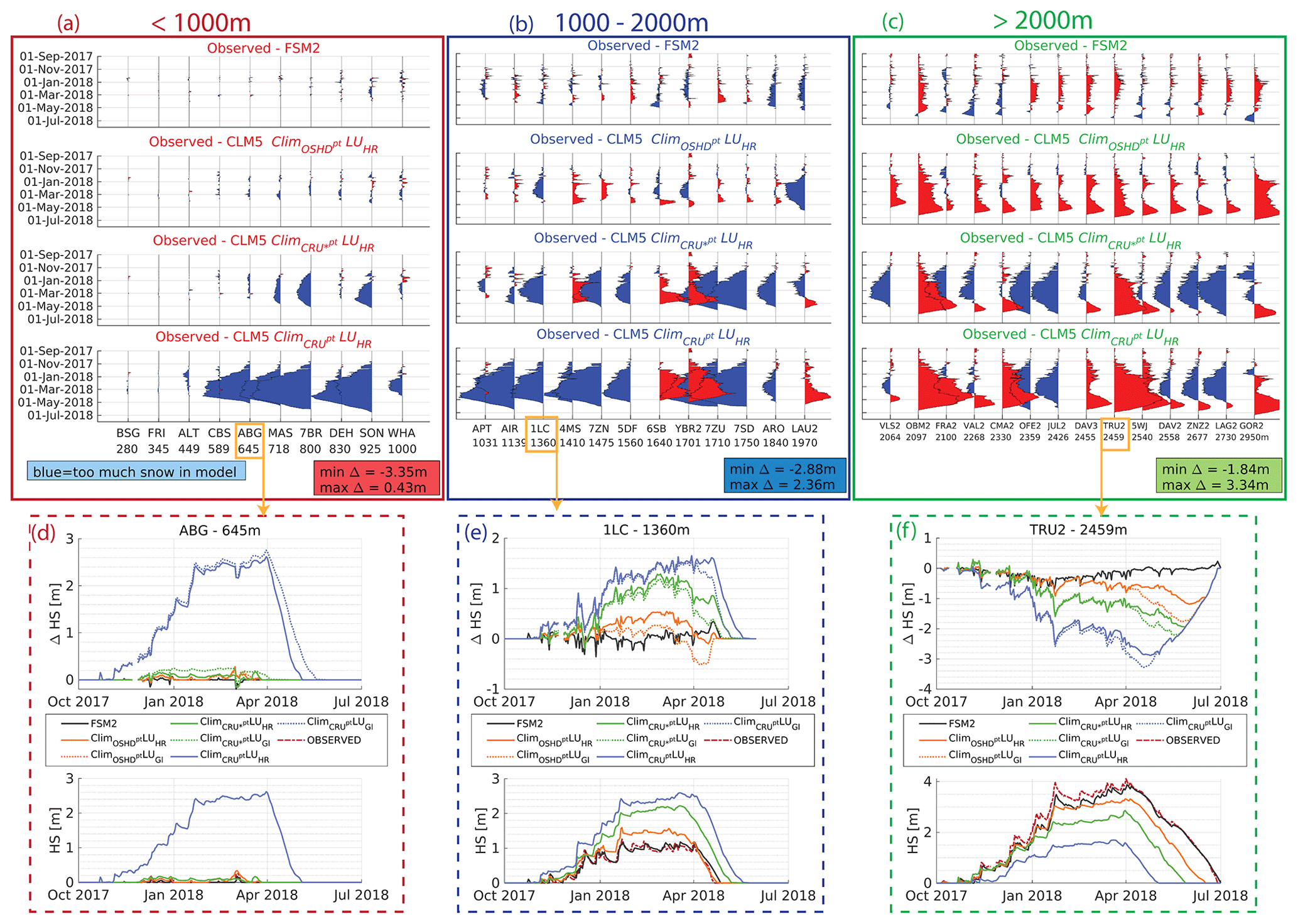
Figure 3 Wiggle plots comparing point-scale model simulations to observations of snow depth (HS) throughout the 2017/18 season for low-elevation (a), mid-elevation (b) and high-elevation (c) point locations, where blue denotes too much snow and red too little snow in the models when compared to observations. (d–f) Absolute difference from observations and seasonal snow depth development for three example point locations.

When the lapse-rate-based downscaled temperature input was used (Clim${}_{{\text{CRU*}}^{\mathrm{pt}}}$ + LU_Gl/HR/nofor) instead, the model's performance improved significantly, particularly at low elevations. At mid and high elevations the positive impact of a better temperature representation is masked by the overestimated precipitation input when compared to the OSHD dataset (see Figs. C2 and C4 for a comparison of precipitation forcing between the CRU and the OSHD forcing dataset). The overestimation of snow at mid and high elevations of the Clim_CRU* dataset is hence a direct result of overestimated precipitation along the Alps.

The CLM5 model forced with OSHD data (Clim${}_{{\text{OSHD}}^{\mathrm{pt}}}$ + LU_Gl/HR/nofor) demonstrated the best performance across all three elevation bands, with only minor errors in low- and mid-elevation locations (e.g. RMSE and MAE of 0.22 and 0.11 m, respectively, for mid-elevation Clim${}_{{\text{OSHD}}^{\mathrm{pt}}}$ + LU_HR simulations). These simulations overcome the “too much solid precipitation problem” outlined above as the OSHD precipitation forcing dataset is optimized by data assimilation. The underestimation at high elevations is likely due to snow process representation in the model (combination of snow settling too fast and melting too efficiently; see Fig. 3f). Generally, these results indicate that the CLM5 model forced with OSHD data approach the accuracy of a dedicated snow model (FSM2), at least when assessed at point locations.

Figure 3 further illustrates these results, as it features wiggle plots and seasonal snow development for selected snow station location throughout the 2017/18 winter season. It is apparent across all elevation bands that FSM2 simulations match observations the closest (discussed in more detail in Sect. 3.2) and that CLM5 forced with OSHD data is the next best. CLM5 with global meteorological forcing data (Clim${}_{{\text{CRU}}^{\mathrm{pt}}}$) performs poorly with maximal errors of over 3 m. These biases are persistent throughout the snow season, whereas snow depth is mostly overestimated and underestimated below and above 2000 m, respectively.

Regarding the effects of the land use information dataset, we observed that the choice of land use information only had a small impact on simulated snow depth (Fig. 2). We include simulations using the global, the high-resolution, and the non-forested land use dataset (LU_Gl, LU_HR, LU_nofor, respectively). While a slight improvement was seen when using the high-resolution land use information dataset (LU_HR) at high elevations for all three sets of meteorological forcing data (reducing RMSE by −0.06 m/−0.02 m/−0.11 m for Clim_CRUpt/Clim${}_{{\text{CRU}}^{*}\mathrm{pt}}$/Clim_OSHDpt simulations, respectively), no substantial differences or marginal decreases in model performance were observed for the lower two elevation bands. This is further underlined by Fig. 3d–f. Simulating open, non-forested sites (LU_nofor) only had marginal effects on model performance. For low and mid elevations a slight decrease in model performance is apparent for all three meteorological forcing datasets, whereas at high elevations differences are virtually non-existent. This can be explained by the larger variety in land unit distributions at lower elevations, while at high elevations differences between the two datasets remained small. Ultimately, it can be seen that at coarse model resolution the effect of meteorological forcing data is substantially larger in comparison to differences arising from the choice of land surface information.

3.2 Accuracy of FSM2 point-scale simulations

Across all elevation bands, the FSM2 simulations closely matched the observations, with only minor errors at low and mid elevations during the 2017/18 season (Fig. 2). At high elevations, the FSM2 model slightly underestimated snow depths, which can be assessed in more detail in Fig. 3. Figure 3 visualizes the superior performance of FSM2 in comparison to all CLM5 model experiments, further justifying using FSM2 model simulations as our ground truth for the gridded simulation comparisons in Sect. 3.3.

3.3 Evaluation of gridded snow simulations

The comparison of gridded simulations with CLM5 to FSM2 reference simulations allows us to investigate all three facets of this study: effects of resolution, effects of meteorological forcing data, and effects of land use information data. To this end, we consider gridded simulations of snow depth from all 12 different CLM5 configurations (see Fig. 1ii and iii) and compare them to FSM2 simulations (Fig. 4). Our analysis is performed across all four snow seasons and at 0.25°. Additionally we investigate how the accuracy of CLM5 varies as a function of elevation by comparing all 1 km simulations against FSM2 (Fig. 5) for the 2018/19 season. For both analyses we differentiate between early accumulation period (1 December), mid-accumulation period (1 February), and ablation period (1 April).

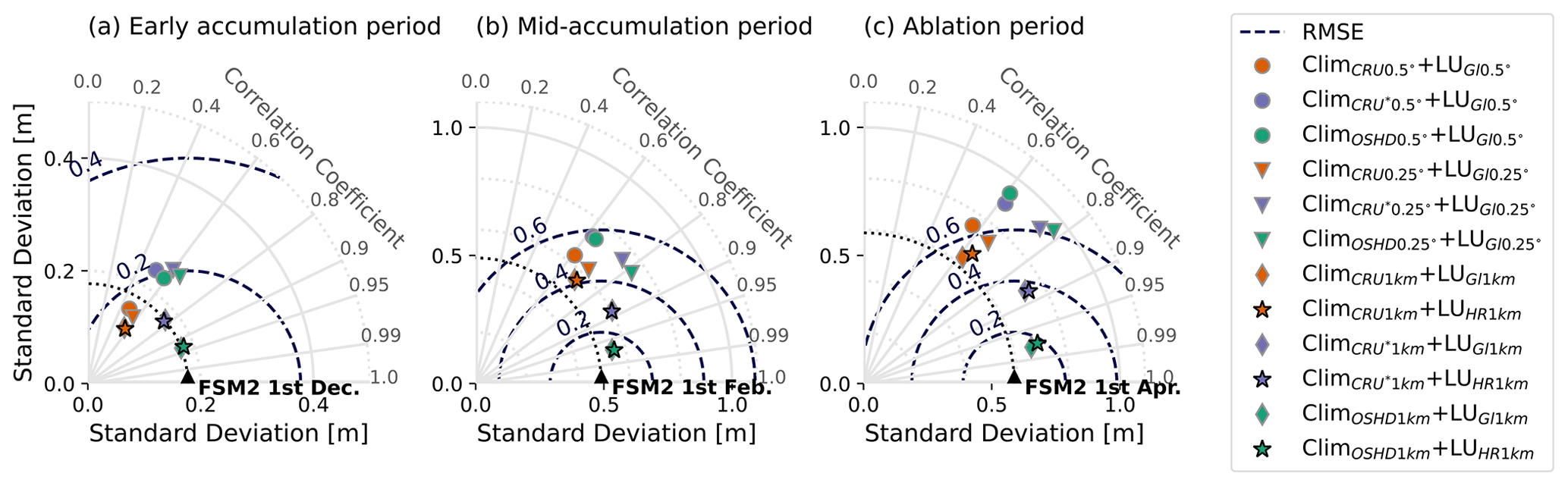
Figure 4 Taylor plots (Taylor, 2001) for comparisons of simulated snow depth (HS) between all 12 different CLM5 configurations and the reference snow simulation (FSM2, dark grey) during the (a) early accumulation season (1 December), (b) mid-accumulation period (1 February), and (c) ablation period (1 April) throughout four winter seasons (2015/16, 2016/17, 2017/18, 2018/19). The plotted statistical metrics allow for evaluation and quantification of CLM5 model experiments performance based on centred RMSE (directly proportional to the distance away from the reference (= FSM2)), correlation coefficients (azimuthal position), and the spatial and temporal standard deviation (radial position from the origin) that determines overestimation or underestimation of the models.

Increasing the level of detail in meteorological forcing data has the largest effect on accuracy of simulated seasonal snow cover, especially when simulating at 1 km. CLM5 runs with OSHD-based input data outperform all CRU- and CRU^*-based simulations at all three points in time during winter (e.g. RMSE Clim_OSHD1 km + LU_Gl1 km of 0.07, 0.14, and 0.18 m; RMSE Clim${}_{{\text{CRU}}^{*}\mathrm{1}\mathrm{km}}$+LU_Gl1 km of 0.12, 0.29, 0.37 m; and RMSE Clim_CRU1 km+LU_Gl1 km of 0.15, 0.41, and 0.53 m for early, mid, and late winter, respectively; Fig. 4)) as compared to FSM2 simulations. The positive effects of lapse-rate-corrected temperatures on model performance (Clim_CRU1 km vs. Clim${}_{{\text{CRU}}^{*}\mathrm{1}\mathrm{km}}$) are pronounced during the mid-accumulation and ablation period, where performance is substantially enhanced, while during the early accumulation only correlation and standard deviation are improved when moving from Clim_CRU1 km to Clim${}_{{\text{CRU}}^{*}\mathrm{1}\mathrm{km}}$. The reason behind this is that during the early season snow height tends to be small anyway, but once snow amounts become substantial the effect of a lapse rate correction in the context of partitioning precipitation into rain and snowfall becomes more evident, and simulation results diverge. A simple lapse rate correction that accounts for high-resolution topography thus already provides many benefits relative to a coarse-resolution dataset.

Figure 5 further illustrates these findings. Focusing in on only one representative season (2018/19) and looking at simulated snow depth as a function of elevation, elevational behaviour of FSM2 is matched closest by CLM5 simulations using OSHD-based forcing data, with most discrepancies occurring during the ablation period at high elevation. Downscaling temperature has a substantial effect on performance, allowing Clim${}_{{\text{CRU}}^{*}\mathrm{1}\mathrm{km}}$ to closely match performance of Clim_OSHD1 km.

However, the benefits of a higher level of detail in the meteorological forcing are negated when model resolution itself is decreased. Comparing results of CLM5 configurations that differed in resolution only, a large decrease in accuracy is evident for the OSHD- and CRU^*-based runs when moving from 1 km to 0.25°, while further coarsening to 0.5° only has a marginal effect. This is because the evolution of snow cover is shaped by non-linear process interactions (e.g. temperature fields affect both snowpack energetics and its mass balance by dictating precipitation phase) that are “lost” when meteorological input is averaged spatially. Our simulations suggest that a model resolution higher than 0.25° is essential to capture the spatial heterogeneity of snow cover evolution processes in the complex terrain present in our study domain. In accordance with this finding, resolution did not have much impact on the performance of the CRU-based runs, since simple regridding without additional consideration of topographic effects on the meteorological drivers does not bring any added value in capturing the non-linear processes shaping snow cover dynamics in complex terrain.

Ultimately, substantial differences in simulated snow cover between the various CLM5 configurations are evident throughout the 4 modelled years and averaged over the model domain (Fig. 4). In a similar manner to the point-scale CLM5 simulations, results revealed considerable improvements in simulated snow cover accuracy when using high-confidence forcing data (Figs. 2, 4), with CLM5 in our best-effort scenario (Clim_OSHD1 km + LU_HR1 km simulation) almost reaching the level of a dedicated snow model also in a gridded application. This becomes especially apparent when looking at the high correlation coefficient of the Clim_OSHD1 km + LU_HR1 km simulation in Fig. 4. However, degraded model performance between the 1 km and the 0.25° configurations suggests that in order to actually benefit from the added value of high-quality forcing data, a sufficiently high model resolution remains necessary when applying CLM5 in topographically complex regions.

In order to better understand why the effect of land use data in our results was minimal, we further investigated the link between changes in land use information and simulated snow cover for non-forested vs. forest-dominated grid cells. Figure 6 compares differences in PAI (averaged across all PFTs, averaged between January–March) across the model domain between LU_HR1 km and the LU_Gl1 km with simulated snow height for 1 February 2018. We show that the majority of snow-dominated pixels correspond to pixels with little change in PAI between the high-resolution and the global land use datasets (e.g. non-forested areas). Pixels with large changes in PAI on the contrary tend to be located in the lowlands, with little snow throughout the season. This demonstrates that the impact of land use data is masked by the many pixels with much snow but little change in PAI. The low sensitivity we find with regards to land use forcing is hence mostly a symptom of the limited overlap between snow-dominated and forested areas in our model domain.

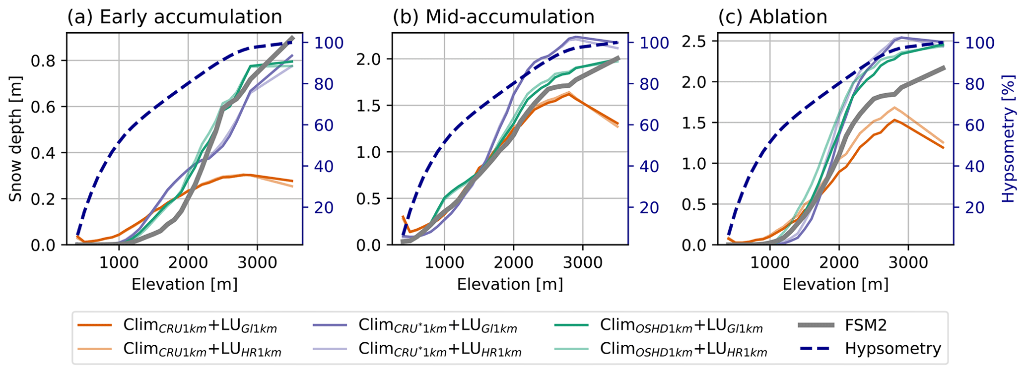
Figure 5 Simulated snow depth (HS) as a function of elevation during the (a) early accumulation season (1 December), (b) mid-accumulation period (1 February), and (c) ablation period (1 April) for the 2018/19 winter season. We contrast the elevational dependency of FSM2 (dark grey) with all six 1 km CLM5 configurations. The dashed dark blue line represents hypsometry across the model domain (Switzerland+).

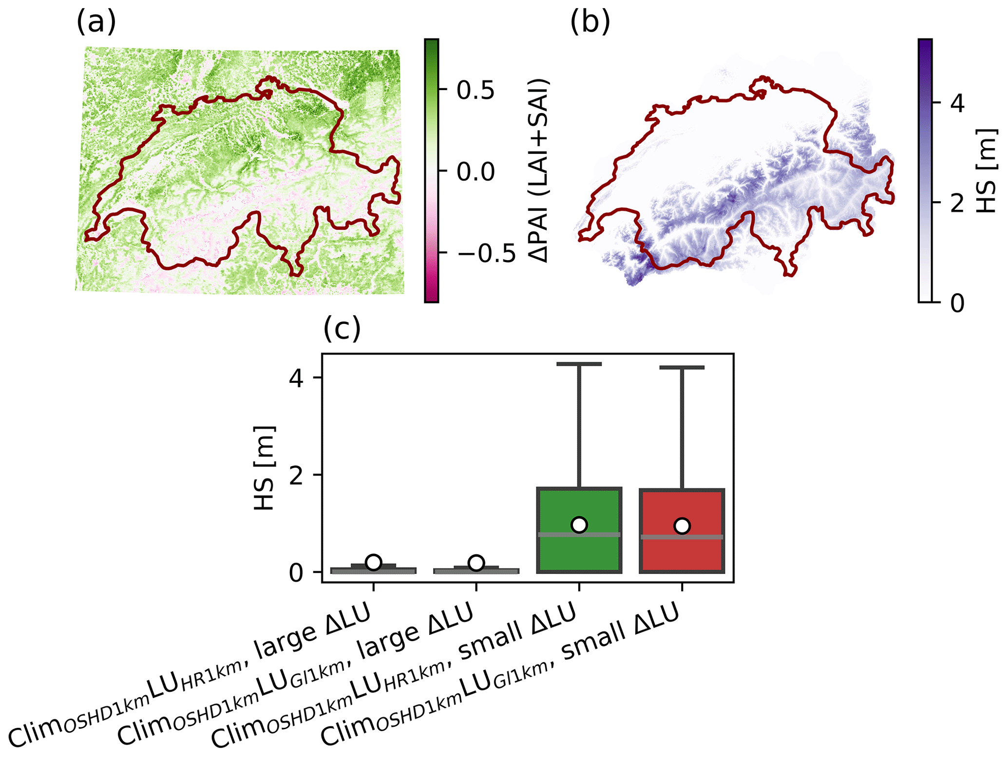
Figure 6 Links between change in land use and simulated snow cover: (a) PAI difference between the LU_HR1 km and LU_Gl1 km dataset, whereby PAI (LAI + SAI) is averaged across all PFTs and between January and March. (b) Snow depth on 1 February 2018 as simulated by CLM5 Clim_OSHD1 km + LU_HR1 km. (c) Comparison of snow height distributions on 1 February 2018 for Clim_OSHD1 km + LU_HR1 km and Clim_OSHD1 km + LU_Gl1 km, showing data for pixels with a large change in overall PAI (>0.25) and a small change in overall PAI (<0.25).

3.4 Simulation of ecophysiological variables

While the previous sections focused on the representation of snow cover, an asset of LSMs relative to dedicated snow models such as FSM2 is that they include a more comprehensive description of land surface processes and state variables, allowing the interaction between these to be investigated. In this final part of our analysis, we thus extend our focus to ecophysiological parameters to showcase effects of spatial resolution, meteorological forcing, and land use information beyond snow cover. Due to the lack of a reference model for evaluation, we present a relative comparison between spatially distributed (a) simulated mean total GPP for 2016–2019 and (b) total ET during 2017 in Fig. 7. To single out the impact of each facet of our study, in each plot Clim_OSHD1 km + LU_Gl1 km is compared with the Clim_OSHD1 km + LU_HR1 km simulation (effect of land use information), with the Clim_CRU1 km + LU_Gl1 km (effect of meteorological forcing), and with the Clim_OSHD0.5° + LU_Gl0.5° simulation (effect of spatial resolution).

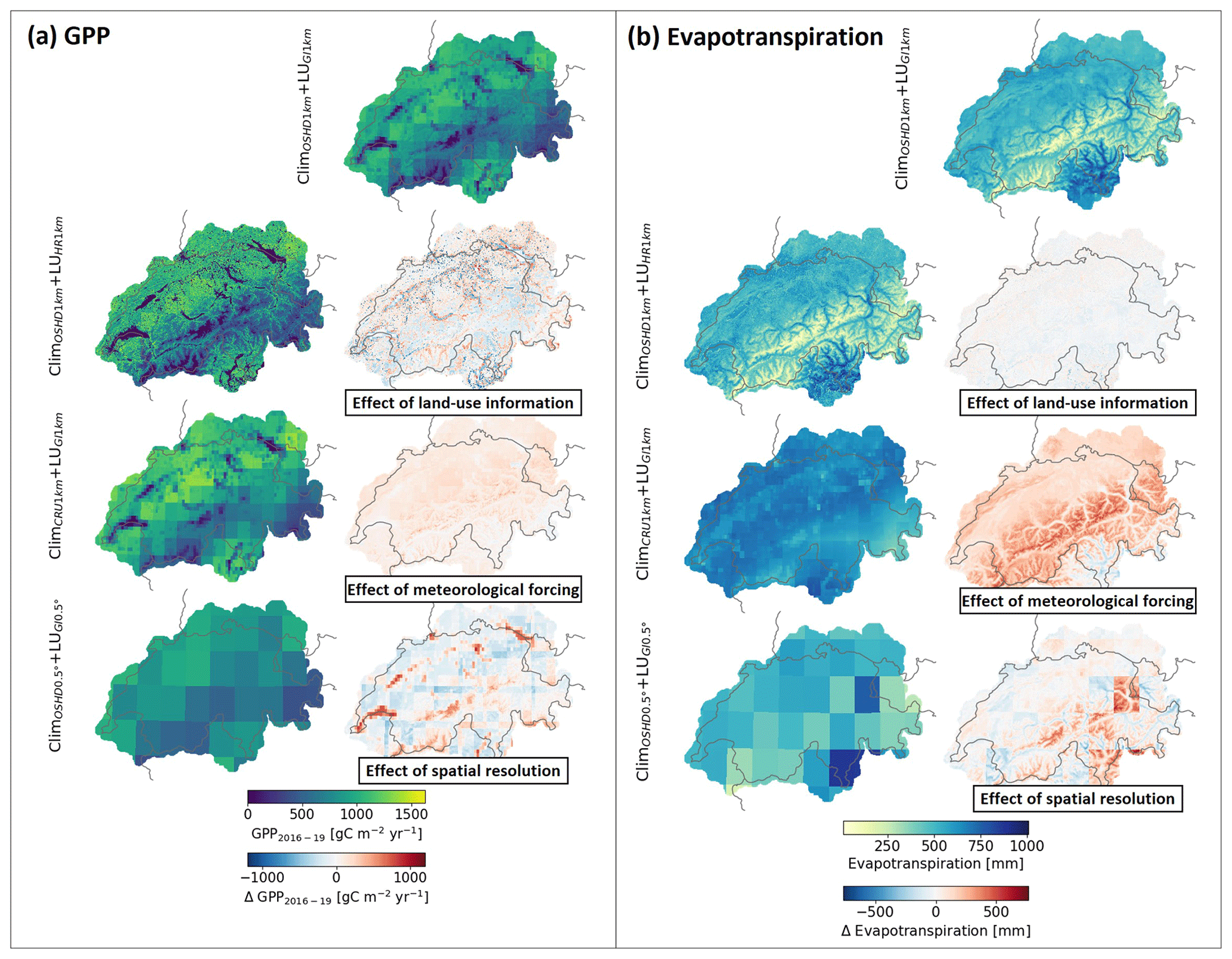
Figure 7 Spatial comparison of CLM5-simulated (a) yearly GPP (mean 2016–2019) and (b) evapotranspiration for four different CLM5 configurations of this study, showing absolute values and relative differences to investigate the effect of land use information, the effect of climatological forcing, and the effect of spatial resolution.

For GPP, sensitivity of land use information outweighed sensitivity of meteorological forcing. The higher level of detail in the land use data caused both increases and decreases in GPP across the model domain, while improved meteorological input had a more systematic effect.

The choice of land surface information datasets, on the other hand, only showed marginal effects on simulated ET, but the effect of meteorological forcing results in substantial differences in simulated ET (up to 26 % when averaged over the entire model domain). This effect is especially pronounced along the Swiss Alps, where complex terrain leads to differences in precipitation patterns captured by the two forcings (see Figs. C2, C4, and C3 for comparison of precipitation patterns in the forcing datasets). Temperature differences between the two forcing datasets further contributed to the differences, as it is precisely along the Swiss Alps where Clim_CRU1 km does not capture topographic effects on temperature.

For both GPP and ET, model resolution in isolation strongly affects the spatial patterns due to non-resolved surface heterogeneity at coarse resolution. Discrepancies between the simulations are less directional and hence difficult to quantify.

4 Discussion

This study used CLM5 to offer a multi-scale assessment of the representation of seasonal snow in complex topographic terrain by evaluating simulated snow depth against a wealth of station data, as well as gridded FSM2 simulations. The multi-resolution setup and a suite of model experiments allowed assessment of several aspects (impact of resolution and input datasets) in a spatially and temporally resolved manner, while leveraging diverse reference datasets.

Evaluation against station data showed that CLM5 itself is capable of achieving performance similar to a dedicated snow model when applied in point mode and with the best available input data (land use info and meteorological forcing; Clim_OSHD1 km + LU_HR1 km). Differences from station data are largest at high elevation, where CLM5 underestimates snow cover. As this bias persists throughout the season, it is likely due to a combination of accumulation and internal snowpack properties (e.g. the settling parameterization) and melt processes. Tracking down the exact mechanism would require a process-level comparison beyond the scope of this study, but it should be noted that in FSM2 (as set up by OSHD) parameters such as the effective roughness length and fresh snow albedo vary spatially (e.g. with elevation); future studies could assess whether such spatially variable parameters could benefit CLM5 snow simulations as well.

Rather than point-mode applications, however, CLM is intended for gridded applications over large areas. This is where our modelling experiments provided interesting insights into the performance of different CLM5 configurations. We found that the most accurate snow cover simulations for Switzerland, with results comparable to those of the operational snow-hydrological model (FSM2), were achieved using high-resolution meteorological forcing data (OSHD) and a 1 km resolution that fully resolved landscape heterogeneity. This confirmed our hypothesis, which stated that with increasing spatial resolution and quality of meteorological and land surface input datasets, the representation of snow cover dynamics and its associated variables in CLM5 can achieve an accuracy comparable to that of a dedicated snow model. These findings align with previous studies (e.g. Lüthi et al., 2019).

Performance of snow cover simulations is thus constrained by the capability of the meteorological input to capture topographic effects (e.g. improved estimation of precipitation phase due to the high-resolution temperature fields) and precipitation patterns, which is a function of both input type (e.g. Clim_OSHD vs. Clim_CRU) and model resolution. Indeed, the fact that aggregating OSHD-based forcing data for coarser-resolution simulations drastically reduced simulation accuracy evidenced the need for resolutions higher than 0.25° for snow simulations in topographically complex terrain.

The lapse-rate-corrected results (Clim${}_{{\text{CRU}}^{*}}$) suggest that in the absence of native high-resolution input data, increasing model resolution through interpolation of input fields with a simple lapse-rate correction of temperature fields can already account for an important topographic effect and thus positively impact model results. This approach, however, cannot provide the high-quality precipitation data achieved with data-assimilation-based techniques (as used in the OSHD forcing). Model errors are thus inherently linked to uncertainty in precipitation input, which can cause both overestimations and underestimations of snow (in the case of the evaluation at the stations, errors in precipitation (overestimation) overcompensated the underestimation seen in the Clim_OSHD simulations for the highest elevation band).

Where model simulations at high resolution are unfeasible (e.g. limited by computational constraints), results from our study suggest that developing a sub-grid parameterization that accounts for the impact of topography on precipitation partitioning and temperature could be a promising approach.

Snow simulations were not sensitive to land use data, but this is likely due to the distribution of land units within our model domain, as most snow-dominated grid cells only saw small changes when moving from the global (LU_Gl1 km) to the high-resolution land use dataset (LU_HR1 km). Previous multi-resolution studies with FSM2 have shown that land use data does indeed affect simulated snow dynamics (Mazzotti et al., 2021). However, for other ecophysiological variables (GPP in this case) we showed a large effect of land use data. Today, a plenitude of new detailed land cover datasets are emerging thanks to advances in satellite remote sensing datasets, which should be exploited for land surface modelling.

To gain a more comprehensive understanding of this topic, it would be beneficial to repeat such a model experiment in an arctic environment rather than just an alpine one, as high latitudes are critical components of the rapidly changing climate system. Changes in land use datasets are likely to have a greater effect in such environments, as larger extents of forested areas overlap with seasonally snow-covered areas.

Additionally, it is important to note that all simulations in this work were conducted in satellite phenology mode. Direct assessments of linkages between simulated snow cover and ecophysiological parameters were hence not possible. Future studies should compare CLM5 simulations with prognostic vegetation and biogeochemistry modes turned on to enable a more detailed analysis of the terrestrial carbon and nitrogen cycles, as well as evapotranspiration fluxes.

Uncertainty remains in climate change impact assessments using LSM projections (e.g. Shrestha et al., 2022; Yuan et al., 2021, 2022), with two major sources of uncertainty being the effects of resolution and the quality of meteorological input data (especially precipitation, Peters-Lidard et al., 2008) on LSM simulation outputs. Quantifying such uncertainties is imperative to further increase the predictive power of climate impact models. Furthermore, given the complexity of state-of-the art LSMs, an understanding of the ways different parts and modules of LSMs interact with each other is more important than ever, as climate change impacts are not isolated but are highly interconnected processes (Zscheischler et al., 2018; Ridder et al., 2021). It is therefore of great importance to investigate how exchanges and interactions between model components are represented, rather than assessing process representation for each model component separately (Blyth et al., 2021), which ultimately requires multidisciplinary community efforts (Ciscar et al., 2019). Multi-resolution modelling frameworks as used for this study have large potential to help with such endeavours and provide critical insights into ecosystem responses to environmental change. More specifically, it can help identify both the key processes for which high-spatial-resolution and high-fidelity input data are necessary, as well as quantify the minimum resolution needed to resolve these processes accurately. Such modelling experiments should be prioritized in the future, ideally in combination with experimental manipulations (e.g. increase the availability of nitrogen or carbon dioxide in the system), as suggested by Wieder et al. (2019).

5 Conclusions

Using multi-resolution modelling experiments to quantify and potentially constrain uncertainties in land surface modelling, we highlight the importance of input data quality and spatial resolution in accurately representing seasonal snow cover across scales. We found that CLM5 is capable of achieving performance similar to a dedicated snow model when using high-resolution meteorological forcing data and a 1 km resolution that represented landscape heterogeneity well. Results further showed that a simple lapse-rate correction of temperature fields can already account for an important topographic effect on precipitation partitioning and has large positive impacts on model performance. Aggregating high-resolution forcing data for coarser-resolution simulations drastically reduced simulation accuracy, further underlining the need for resolutions higher than 0.25° for snow simulations in topographically complex terrain. Snow simulations were less sensitive to land use data compared to meteorological data, but eco-physiological variables (GPP) are strongly affected by the choice of land use forcing. The results clearly demonstrate the utility of high spatial resolution and regionally detailed forcings in land surface models to better quantify and constrain the uncertainties in the represented processes, with profound implications for climate impact studies. More generally, this study highlights the utility of multi-resolution modelling experiments that bridge the gap between point-scale and spatially distributed land surface modelling.

Appendix A: Point-scale CLM5 model simulations at snow stations

Table A1 Name, location, and elevation of all snow station locations used in this study. The last column additionally shows maximum measured snow depth at each station during the 2017/18 winter season.

Appendix B: Land use information datasets

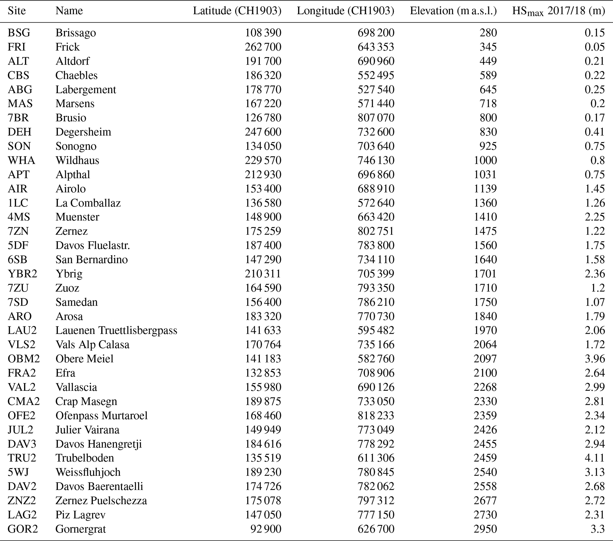
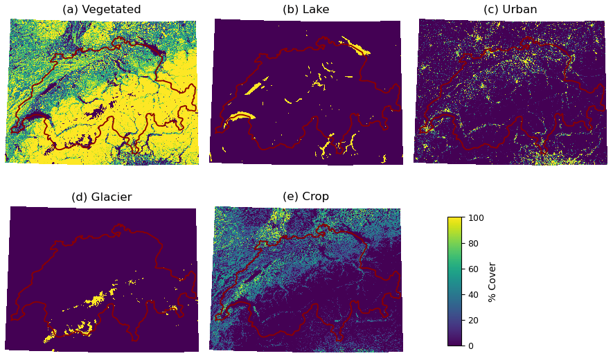
Figure B1 Land unit distribution per grid cell for the high-resolution 1 km land use dataset (LU_HR1 km) as used in this study. The five CLM5 land units sum up to exactly 100 %.

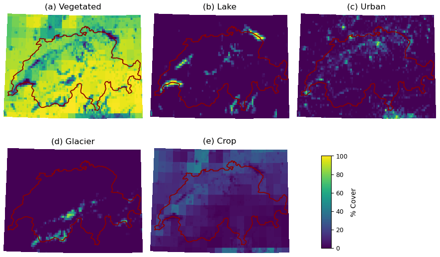
Figure B2 Land unit distribution per grid cell for the global 1 km land use dataset (LU_Gl1 km) as used in this study. The five CLM5 land units sum up to exactly 100 %.

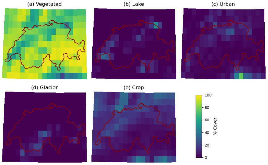
Figure B3 Land unit distribution per grid cell for the global 0.25° land use dataset (LU_Gl0.25°) as used in this study. The five CLM5 land units sum up to exactly 100 %.

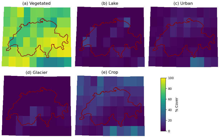
Figure B4 Land unit distribution per grid cell for the global 0.5° land use dataset (LU_Gl0.5°) as used in this study. The five CLM5 land units sum up to exactly 100 %.

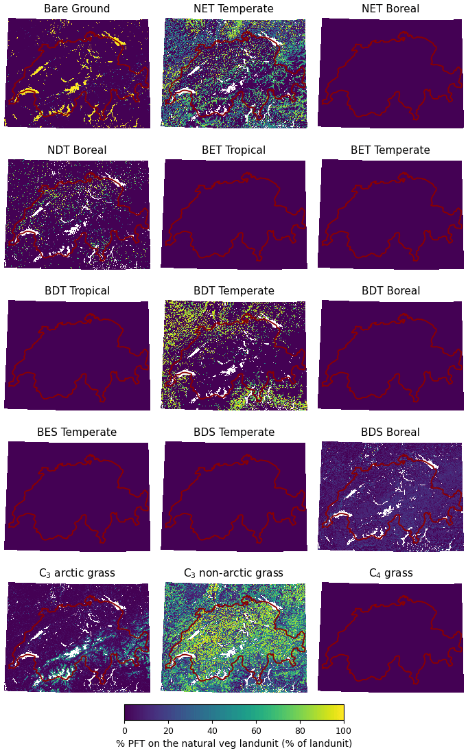
Figure B5 Patch-level plant functional type (PFT) distributions for the high-resolution 1 km land use dataset (LU_HR1 km) as used in this study.

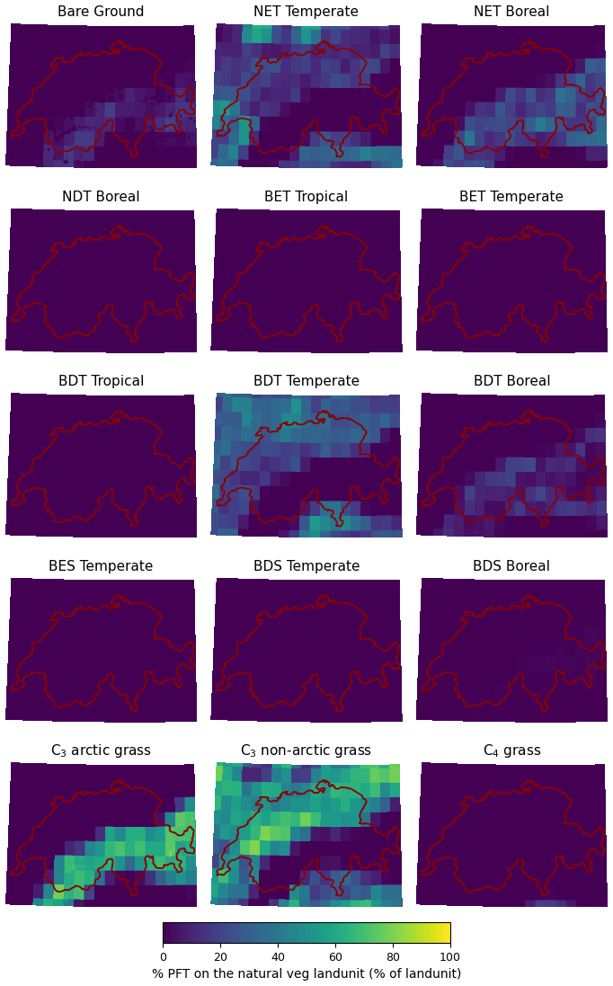
Figure B6 Patch-level plant functional type (PFT) distributions for the global 1 km land use dataset (LU_Gl1 km) as used in this study.

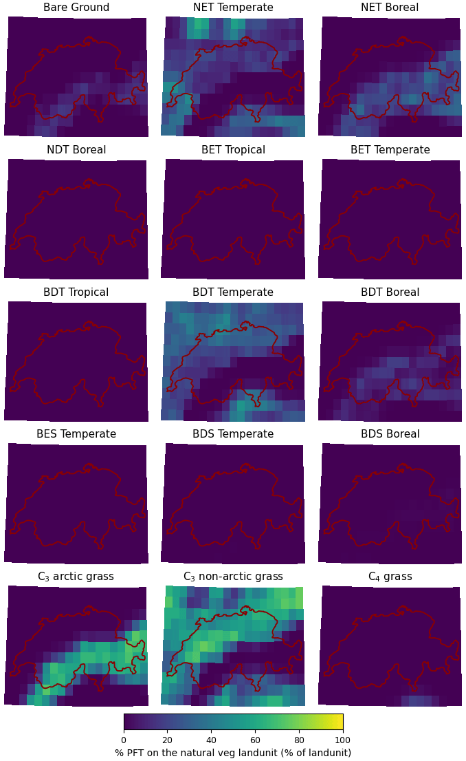
Figure B7 Patch-level plant functional type (PFT) distributions for the global 0.25° land use dataset (LU_Gl0.25°) as used in this study.

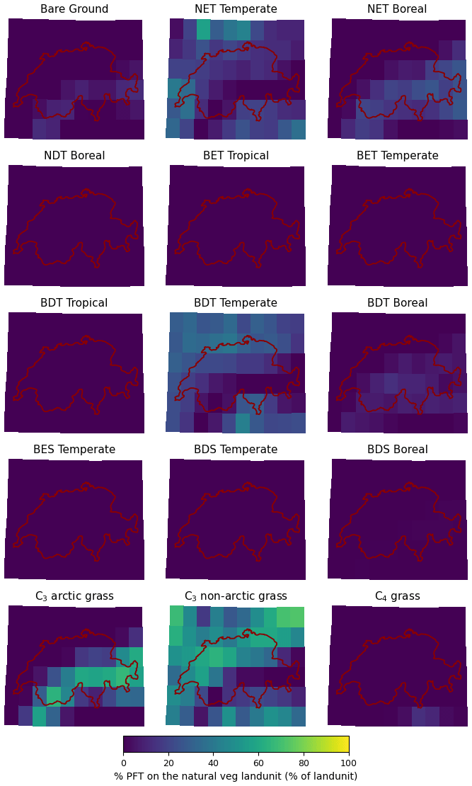
Figure B8 Patch-level plant functional type (PFT) distributions for the global 0.5° land use dataset (LU_Gl0.5°) as used in this study.

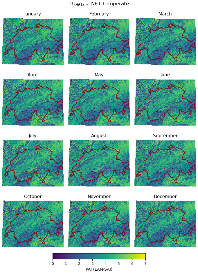
Figure B9 Monthly plant area index (PAI) for temperate needle-leaf evergreen trees for the high-resolution 1 km land use dataset (LU_HR1 km) as used in this study.

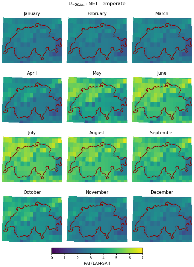
Figure B10 Monthly plant area index (PAI) for temperate needle-leaf evergreen trees for the global 1 km land use dataset (LU_Gl1 km) as used in this study.

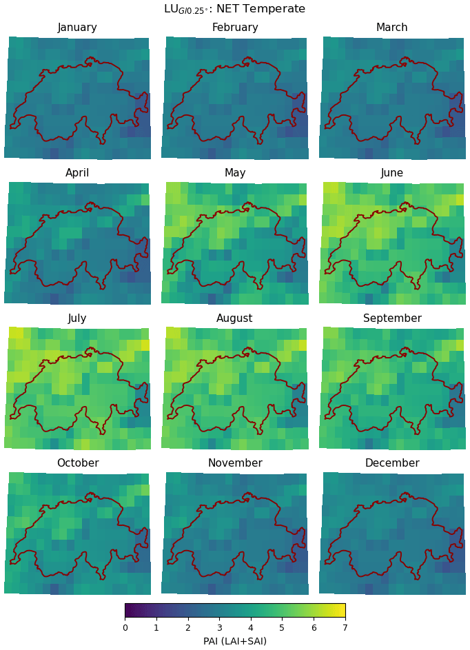
Figure B11 Monthly plant area index (PAI) for temperate needle-leaf evergreen trees for the global 0.25° land use dataset (LU_Gl0.25°) as used in this study.

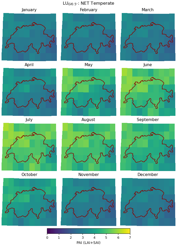
Figure B12 Monthly plant area index (PAI) for temperate needle-leaf evergreen trees for the global 0.5° land use dataset (LU_Gl0.5°) as used in this study.

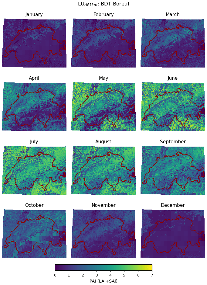
Figure B13 Monthly plant area index (PAI) for boreal broadleaf deciduous trees for the high-resolution 1 km land use dataset (LU_HR1 km) as used in this study.

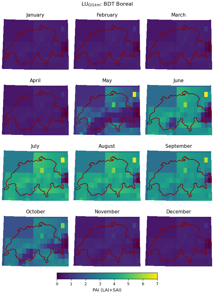
Figure B14 Monthly plant area index (PAI) for boreal broadleaf deciduous trees for the global 1 km land use dataset (LU_Gl1 km) as used in this study.

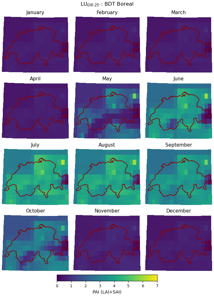
Figure B15 Monthly plant area index (PAI) for boreal broadleaf deciduous trees for the global 0.25° land use dataset (LU_Gl0.25°) as used in this study.

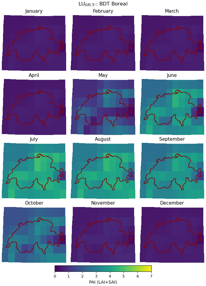
Figure B16 Monthly plant area index (PAI) for boreal broadleaf deciduous trees for the global 0.5° land use dataset (LU_Gl0.5°) as used in this study.

Appendix C: Meteorological forcing data

This section shows supporting information regarding the meteorological forcing data presented in the main part of the paper. First, we show the two DEMs used for lapse rate calculation in this study. We further show differences in yearly and monthly precipitation for the OSHD-based and CRU-based dataset, as well as differences in monthly temperatures between the OSHD-based, the CRU-based, and the Clim${}_{{\text{CRU}}^{*}}$ dataset.

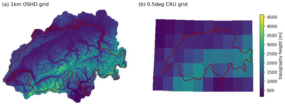
Figure C1 Comparison of digital elevation model (DEM) at (a) 1 km and (b) 0.5° as used for lapse rate correction in this study.

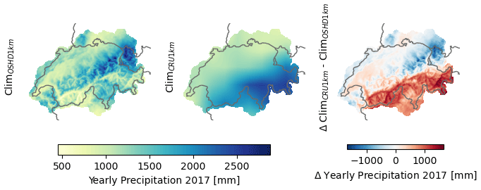
Figure C2 Total yearly precipitation input for the year 2017: OSHD-based dataset, CRU-JRA-based dataset, and a differential plot.

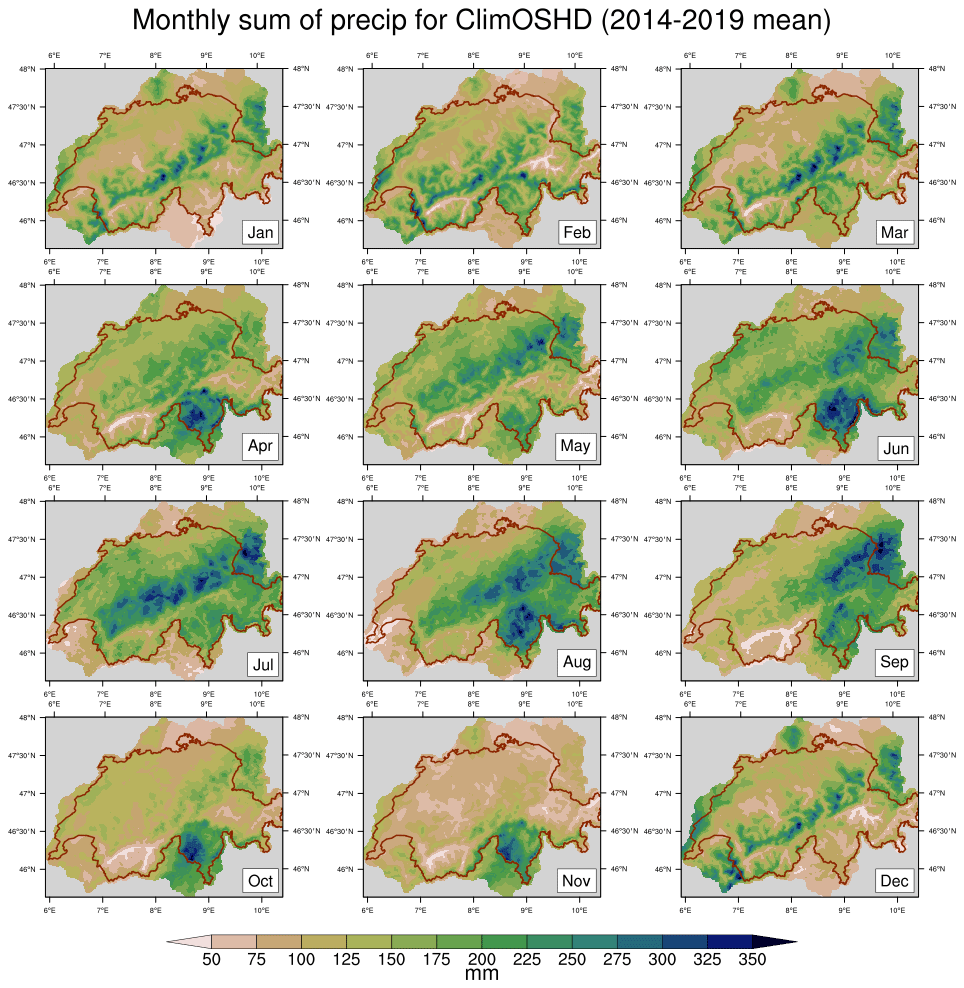
Figure C3 Total monthly precipitation input as averaged between 2014 and 2019 for the Clim_OSHD forcing dataset.

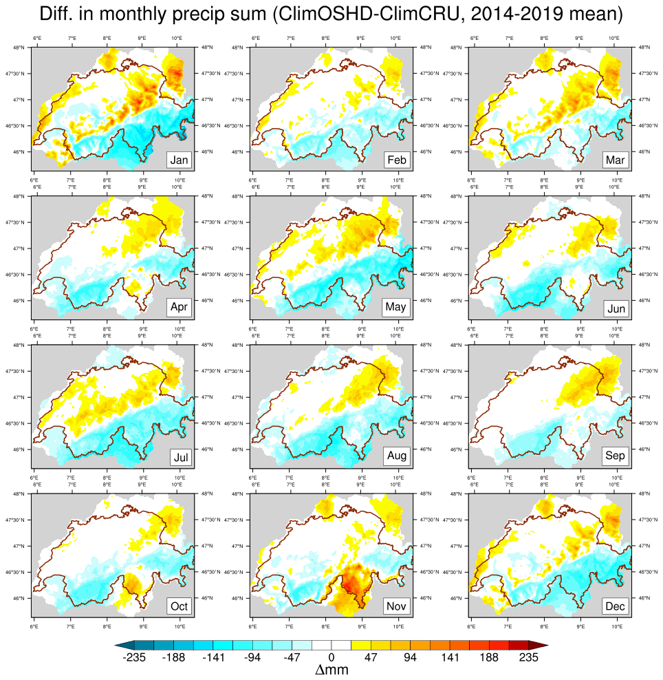
Figure C4 Differences in total monthly precipitation input between the Clim_OSHD and the Clim_CRU forcing dataset.

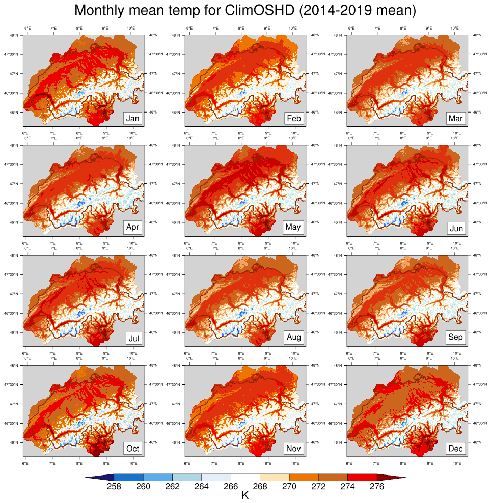
Figure C5 Mean monthly temperatures for the Clim_OSHD forcing dataset.

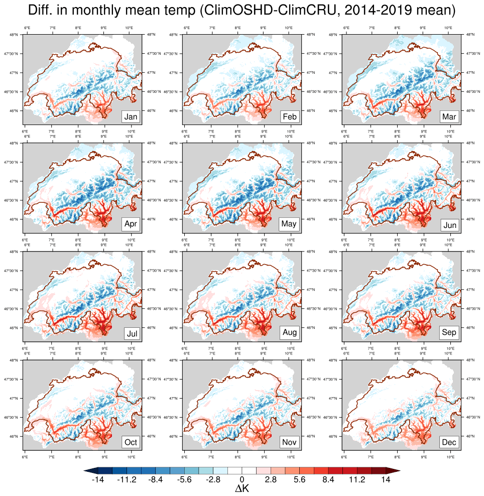
Figure C6 Differences in mean monthly temperatures between the Clim_OSHD and the Clim_CRU forcing dataset.

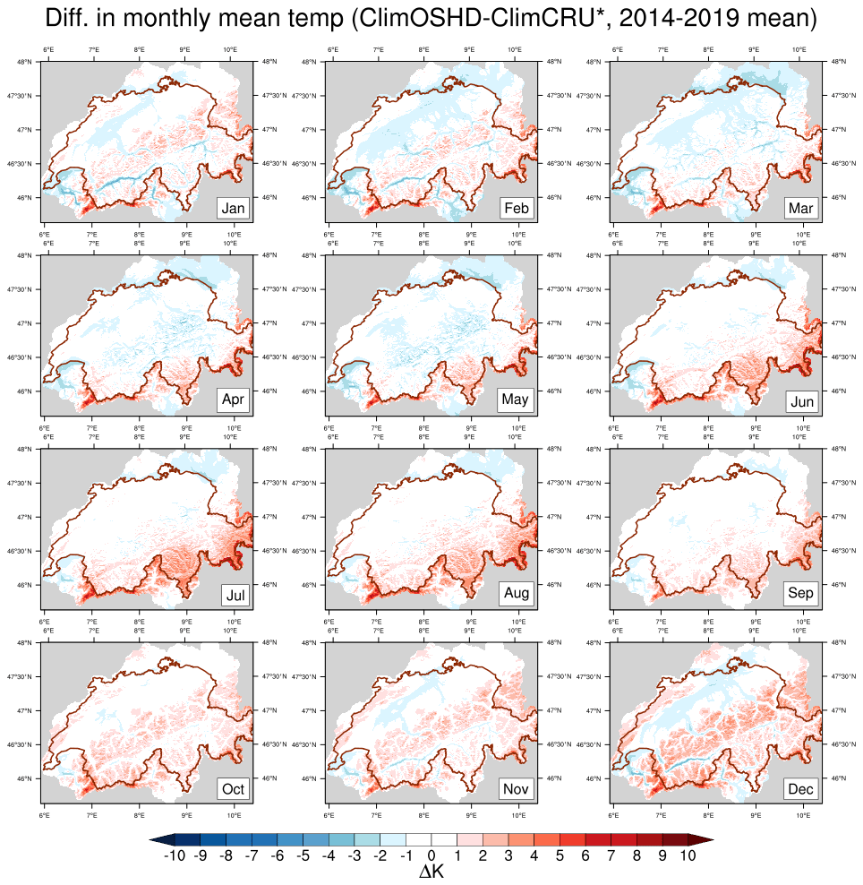
Figure C7 Differences in mean monthly temperatures between the Clim_OSHD and the lapse-rate-corrected Clim${}_{{\text{CRU}}^{*}}$ forcing dataset.

Appendix D: Spatially distributed CLM5 model simulations

This section shows supporting analyses for the spatially distributed CLM5 model simulations presented in the main part of the paper.

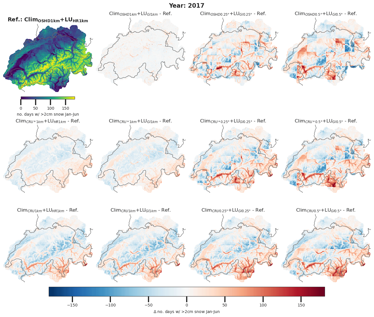
Figure D1 Spatial comparison of the number of days with more than 2 cm snow on the ground between January and June 2017. The reference case (Clim_OSHD1 km + LU_HR1 km) is compared with simulations of all other CLM5 configurations used in this study. For the residual plots, blue indicates underestimation and red overestimation in comparison to the reference case.

Figure D2 Spatial comparison of melt-out date (day of year) during 2017. The reference case (Clim_OSHD1 km + LU_HR1 km) is compared with simulations of all other CLM5 configurations used in this study. For the residual plots, blue indicates underestimation and red overestimation in comparison to the reference case.

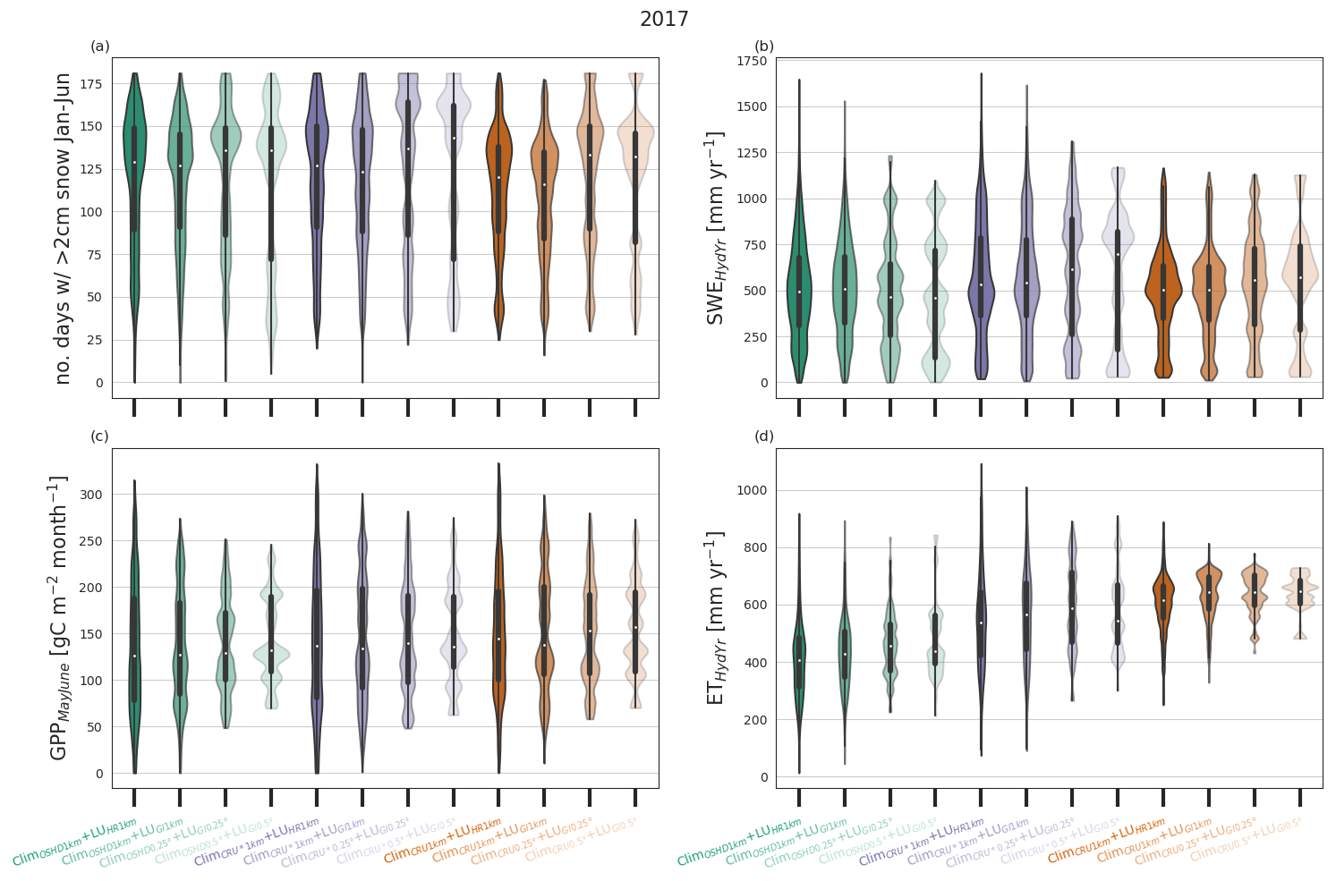
Figure D3 Violin plots showing comparison of all 12 CLM5 model configurations for the year 2017 across the entire model domain: (a) number of days with >2 cm of snow between January and June 2017, (b) cumulative SWE (total positive SWE increments; “how much water is stored in total”) during the hydrological year 2017 (1 October 2016–30 September 2017), (c) monthly averaged GPP during May and June 2017, and (d) total evapotranspiration during the 2017 hydrological year. In addition to information obtained from a box plot (25th + 75th percentiles and median), the violin plots show a kernel density estimate of the data.